A new $F_{\text{ST}}$-based method to uncover local adaptation using environmental variables.

Abstract

• Genome-scan methods are used for screening genome-wide patterns of DNA polymorphism to detect signatures of positive selection. There are two main types of methods: (i) “outlier” detection methods based on $F_{\text{ST}}$ that detect loci with high differentiation compared to the rest of the genomes, and (ii) environmental association methods that test the association between allele frequencies and environmental variables.
• We present a new $F_{\text{ST}}$-based genome-scan method, BayeScEnv, which incorporates environmental information in the form of “environmental differentiation”. It is based on the F model, but, as opposed to existing approaches, it considers two locus-specific effects; one due to divergent selection, and another one due to various other processes different from local adaptation (e.g. range expansions, differences in mutation rates across loci or background selection). The method was developped in C++ and is avaible at http://github.com/devillemereuil/bayescenv.
• Simulation studies shows that our method has a much lower false positive rate than an existing $F_{\text{ST}}$-based method, BayeScan, under a wide range of demographic scenarios. Although it has lower power, it leads to a better compromise between power and false positive rate.
• We apply our method to human and salmon datasets and show that it can be used successfully to study local adaptation. We discuss its scope and compare its mechanics to other existing methods.

Keywords: genome scan, local adaptation, environment, F model, Bayesian methods, false discovery rate

Corresponding author: Pierre de Villemereuil, E-mail: bonamy@horus.ens.fr

Introduction

One of the most important aims of population genomics (Luikart et al., 2003) is to uncover signatures of selection in genomes of non model species. Of special interest is the process of local adaptation, whereby populations experiencing different environmental conditions undergo adaptive, selective pressures specific to their local habitat. As a result, populations evolve traits that provide an advantage in their local environment. Many experimental approaches focused on potentially adaptive traits have been developed to test for local adaptation (reviewed in Blanquart et al., 2013), but only recently it has become possible to make inferences about the genomic regions involved in local adaptation processes. Indeed, the advent of next generation sequencing (NGS, Shendure and Ji, 2008) has fostered the development of so-called genome-scan methods aimed at identifying regions of the genome subject to selection. These methods are now widely used in studies of local adaptation (Faria et al., 2014).

There are two main types of genome-scan methods. The first type detects ‘outlier’ loci using locus-specific $F_{\text{ST}}$ estimates, which are compared to either an empirical distribution (Akey et al., 2002), or to a distribution expected under a neutral model of evolution (Beaumont and Balding, 2004; Foll and Gaggiotti, 2008). The rationale behind these methods is that local adaptation leads to strong genetic differentiation between populations, but only at the selected loci (or marker loci linked to them). Thus, loci with very high $F_{\text{ST}}$ compared to the rest of the genome are suspected to be under strong local adaptation and are referred to as outliers. The outlier approach was further extended to statistics akin to $F_{\text{ST}}$ (Bonhomme et al., 2010; Günther and Coop, 2013), and also to other unrelated statistics (Duforet-Frebourg et al., 2014). One limitation of these methods is that they are not designed to test hypotheses about the environmental factors underlying the selective pressure.

A second type of methods focuses on environmental variables and aims at associating patterns of allele frequency to environmental gradients. The rationale is that selective pressures should create associations between allele frequencies at the selected loci and the causal environmental variables (Coop et al., 2010). In the presence of population structure, performing a simple linear regression would be an error-prone approach (De Mita et al., 2013; de Villemereuil et al., 2014). Instead, existing methods account for population structure by modelling the allele frequency covariation across populations (Coop et al., 2010; Frichot et al., 2013; Guillot et al., 2014). One disadvantage of these approaches is that the parameters that capture the effect of demographic history on genetic differentiation do not have a clear biological interpretation, which in turn makes the rejection of the null model hard to interpret in terms of detection of local adaptation. We note that although the elements of the covariance matrix estimated by Coop et al. (2010) could in principle be interpreted as parametric estimates of the pairwise and population-specific $F_{\text{ST}}$, this is only true when levels of genetic drift are low (Nicholson et al., 2002).

It is important to note that, regardless of the type of genome-scan method under consideration, processes other than local adaptation might be responsible for the observed spatial patterns in allele frequency or $F_{\text{ST}}$. These include demographic processes (e.g. allele surfing; Edmonds et al., 2004), large differences in mutation rate across loci (Edelaar et al., 2011), hybrid incompatibility following secondary contact (Kruuk et al., 1999) and background selection (Charlesworth, 1998). It is therefore possible that some of the loci identified as outliers are in fact false positives. Accounting for processes other than selection would require introducing parameters that could appropriately capture the effect of these other processes.

Here, we present a method that incorporates features of the two types of genome-scans described above. The objective is to better discriminate between true and false genetic signatures of local adaptation, and simultaneously allow inferences about the environmental factors underlying selective pressures. More precisely, our method is based on the Bayesian approach first proposed by Beaumont and Balding (2004) and later extended by Foll and Gaggiotti (2008). The original formulation considers population- and locus-specific $F_{\text{ST}}$’s, which are described by a logistic regression model with three parameters: a locus-specific term, $\alpha_{i}$, that captures the effect of mutation and some forms of selection, a population-specific term, $\beta_{j}$, that captures demographic effects (e.g. $N_{e}$ and migration) and a locus-by-population interaction term, $\gamma_{ij}$, that reflects the effect of local adaptation. The estimation of the first two terms benefits from sharing information across loci or populations, but this is not the case for the interaction term, which is therefore poorly estimated (Beaumont and Balding, 2004, but see Riebler et al., 2008). In practice signatures of local adaptation are therefore inferred from the locus-specific effects ($\alpha_{i}$) under the assumption that large positive values reflect adaptive selection. The implicit assumption is that background selection and mutation should not have much of an effect on this regression term. In order to relax this assumption and to better estimate the interaction term we introduce environmental data so that $\gamma_{ij}=g_{i}E_{j}$, where $E_{j}$ is the “environmental differentiation” observed in population $j$ and $g_{i}$ is a locus-specific regression coefficient. In what follows, we first describe in detail the probabilistic model underlying our Bayesian approach. We then evaluate its performance using simulated data and present an application using human and salmon datasets. Finally, we discuss the scope of our method and compare it with other existing genome-scan approaches.

Statistical model

Modelling allele frequencies using the $F$ model

Our new genome-scan approach is based on the $F$ model (Beaumont and Balding, 2004; Foll and Gaggiotti, 2008) and extends the software BayeScan (Foll and Gaggiotti, 2008) by incorporating environmental data so as to explicitly consider local adaptation scenarios. Full details of the $F$ model are given by Gaggiotti and Foll (2010), so here we only provide a brief description. The core assumptions of the $F$ model is that all populations share a common pool of migrants, but that their effective sizes and immigration rates are population-specific. Thus, population structure at each locus is described by local $F_{\text{ST}}$’s that measure genetic differentiation between each local population and the migrant pool.

The $F$ model uses the multinomial-Dirichlet likelihood for the allele counts $\bm{a_{ij}}=(a_{i,j,1},\dots,a_{i,j,K_{i}})$ at locus $i$ within population $j$ (where $K_{i}$ is the number of distinct alleles at locus $i$) with parameters given by the migrant pool allele frequencies, $\bm{f_{i}}=(f_{i,1},\dots,f_{i,K_{i}})$, and a population- and locus-specific parameter of similarity, $\theta_{ij}=\dfrac{1-F_{\text{ST}}^{ij}}{F_{\text{ST}}^{ij}}$:

$$\bm{a_{ij}}\sim\text{\it multDir}(\theta_{ij}f_{i,1},\dots,\theta_{ij}f_{i,K_{i}}),$$ (1)

where multDir stands for the multinomial-Dirichlet distribution.
Although, for the sake of simplicity, we only present here the formulation for co-dominant data, the software implementing our approach also allows for dominant data (e.g. AFLP markers) using the same probabilistic model as Foll and Gaggiotti (2008). Note finally that, for bi-allelic co-dominant markers (e.g. SNP markers), the likelihood reduces to a beta-binomial model.

Alternative models to explain population structure

Our purpose is to better discriminate between true signals of local adaptation and spurious signals left by other processes. Therefore, we assume that genetic differentiation at individual loci is influenced by three type of effects: (i) genome-wide effects due to demography, (ii) a locus-specific effect due to local adaptation caused by the focal environmental variable, and (iii) locus-specific effects unrelated to the focal environmental variable. Although in principle one could consider all seven alternative model that can be constructed with different combinations of these three effects, most of them would not have any biological meaning. For example, all models should include genome-wide effects associated with genetic drift. Additionally, we do not consider the two types of locus-specific effects simultaneously in a full model. The reason is that the statistical (and hence biological) interpretation of $\alpha_{i}$ will depend on whether or not the parameter $g_{i}$ is included in the model.

This can render the algorithms overly complicated, especially during the pilot runs (see below).

Thus, we focus on three alternative models to explain the genetic structuring at individual loci.

Null model of population structure

Under the null hypothesis that all loci are neutral, the local differentiation parameter $F_{\text{ST}}^{ij}$ will be driven only by local population demography and, hence, should be common to all loci:

$$\log\left(\frac{F_{\text{ST}}^{ij}}{1-F_{\text{ST}}^{ij}}\right)=\log\left(\frac{1}{\theta_{ij}}\right)=\beta_{j}.$$ (2)

A high $\beta_{j}$ value means that the population $j$ is strongly differentiated from the pool of migrants. This could be due to a lack of immigration from the other populations, a reduced effective size, or a particular spatial structure.

Alternative model of local adaptation

In this model, we focus on a particular signature left by a process of local adaptation. If selection is driven by a putative environmental factor, we expect that genetic differentiation for the locus or loci under selection will be stronger than expected under neutrality for populations with strong environmental differentiation. Any measure of distance between the environmental value of population $j$ and the average environment could serve as a measure of differentiation. For the sake of simplicity, we here only consider the absolute value (i.e. Manhattan distance). Its advantage is that it does not over-state the importance of outlier environmental values. Furthermore, in order to facilitate the calibration of prior distributions, we only consider standardised environmental values (i.e. with zero mean and unit variance).
To model the effect of local adaptation on locus $i$, we consider the impact of environmental differentiation $E_{j}$ of population $j$ on the locus, we thus modify Eq. 2 as follows:

$$\log\left(\frac{F_{\text{ST}}^{ij}}{1-F_{\text{ST}}^{ij}}\right)=\beta_{j}+g_{i}E_{j},$$ (3)

where $g_{i}$ quantifies the sensitivity of locus $i$ to the environmental differentiation.

Alternative model of locus-specific effect

Local adaptation with respect to the focal environmental variable is not the only evolutionary phenomenon that could lead to departures from the neutral model. Other phenomena that could produce such locus-specific effects include local adaptation due to other unknown factors, large differences in mutation rate across loci, the so-called allele surfing phenomenon (Edmonds et al., 2004) and background selection (Charlesworth, 2013).

This is accounted for by using the following parametrisation for local differentiation:

$$\log\left(\frac{F_{\text{ST}}^{ij}}{1-F_{\text{ST}}^{ij}}\right)=\alpha_{i}+\beta_{j}.$$ (4)

The main advantage of implementing both of the above alternative models is that we can distinguish between departures from the neutral model of unknown origin (using Eq. 4) and departures due to local adaptation caused by a particular environmental factor (using Eq. 3).

Figure 1: Directed Acyclic Graph (DAG) of the model. Squared nodes denote know quantities ($E$ for environmental data, and $A$ for genetic marker data). Circled nodes denote unknown parameters. Plain arrows stand for deterministic relationships, and dashed arrows stand for stochastic relationships.

Material and Methods

Implementation of the statistical model

Our method uses two types of data: (i) the allele counts $\bm{a}$ for each locus in each population sample, and (ii) observed values $\bm{E}$ of an environmental variable (one value per population), which are transformed into environmental differentiation using an appropriate function. We chose the absolute-value distance, because it allows to weigh down the effect of outlier (i.e. strongly differentiated) environmental values and, therefore, makes the method more conservative. Note that measuring an environmental distance requires to define a reference. The most natural reference would be the average of the environmental values, but this would not be always the case (see the example of adaptation to altitude in humans presented below). Also, it is strongly advised to standardise the environmental values by dividing by the standard deviation, in order to avoid effect size issues regarding the inference of the parameter $g$.
As stated in the previous section, there are three alternative models:

M1

Neutral model: $\beta_{j}$,

M2

Local adaptation model with environmental differentiation $E_{j}$: $\beta_{j}+g_{i}E_{j}$,

M3

Locus-specific model: $\alpha_{i}+\beta_{j}$.

All three models were implemented using an RJMCMC algorithm (Green, 1995). In order to propose relevant values for new parameters during the jumps, the RJMCMC is preceded by pilot runs. These are aimed at both calibrating the MCMC proposals to reach efficient acceptance rates, and approximating the posterior distribution of parameters, as proposed by Brooks (1998) and already implemented in BayeScan (Foll and Gaggiotti, 2008). Our code is based on the source code of BayeScan 2.1 and is written in C++. The source and binaries are available at https://github.com/devillemereuil/bayescenv.
Our prior belief in the three models is described by two parameters: the probability $\pi$ of moving away from the neutral model and the preference $p$ for M3 against M2 as alternative models. We can calculate the prior probability for each model as:

$$\begin{array}[]{rcl}P(\text{{M1}})&=&1-\pi,\\ P(\text{{M2}})&=&\pi(1-p),\\ P(\text{{M3}})&=&\pi p.\\ \end{array}$$ (5)

The details of the mathematical calculation of transition between models can be found in the Supplementary Material. Pilot studies showed that using values of $p$ above 0.5 yielded extremely conservative results.
We used a uniform Dirichlet prior for the allele frequencies $\bm{f}_{i}\sim\text{\it Dir}(1,\dots,1)$. The priors for the hyperparameters $\alpha$ and $\beta$, were Normal with mean -1 and variance 1. Since under a local adaptation scenario the parameter $g$ is only expected to be positive, it was assigned a uniform prior between 0 and 10.

Our method outputs posterior error probabilities and $q$-values, which are test statistics related to the False Discovery Rate (FDR) (Storey, 2002; Käll et al., 2008). Contrary to the commonly used False Positive Rate (FPR), which is the probability of declaring a locus as positive given that it is actually neutral, the FDR is the proportion of the positive results that are in fact false positives, and is more appropriate for multiple testing (Käll et al., 2008). See the Supplementary Information (SI) for more details.

Simulation analysis

We performed a simulation study to evaluate the performance of our method and compare it with that of BayeScan (Foll and Gaggiotti, 2008). We modelled 16 populations each with 500 individuals genotyped at 5,000 loci, among which one (monogenic scenario) or 50 (polygenic scenario) were under selection. We modelled three kinds of population structure: (i) a classical island model (IM), (ii) a one-dimension stepping-stone (SS) model and (iii) a hierarchically structured (HS) model.
The genome was composed of 5,000 bi-allelic SNPs spread along 10 chromosomes. The loci under selection, one for the monogenic case and 50 for the polygenic case, were randomly distributed across the genome. Since all markers were independently initialised, our simulations yielded negligible linkage disequilibrium. Consequently, we considered as true positives only the loci subject to selection. For the IM and SS scenarios, we directly initialised all 16 populations. For the HS scenario, we initialised the ancestral population, which, following successive and temporally spaced-out fission events, gave rise to 2, 4, … , 16 populations. This hierarchical structure is reinforced by preferential migration between related populations. More details regarding migration and population history are available in the SI. This model is very close to that used by de Villemereuil et al. (2014). It should be particularly difficult for our method, because all populations are equally differentiated (i.e. the $\beta_{j}$ parameters are expected to be roughly the same across populations), but a phylo-geographic covariance exists between related populations, which is not explicitly accounted for by our probabilistic model. Information regarding the environmental gradient and the fitness function are available in the SI.
The simulations were performed using the SimuPOP Python library (Peng and Kimmel, 2005) and the scripts are available online in the data section. Our simulated datasets were analysed using our C++ code and version 2.1 of BayeScan (Foll and Gaggiotti, 2008).
We generated 100 datasets for each scenario and computed the realised FDR, FPR and power yielded by BayeScan and our new environmental method (BayeScEnv). For the latter, we also compared several parametrisations using a prior probability $\pi$ of jumping away from the neutral model of $0.1$ (equivalent to the default prior odds used by BayeScan, which is 10) or $0.5$, as well as a preference for the locus-specific model $p$ of 0.5 (environmental and locus-specific models are equiprobable) or 0 (the locus-specific model is forbidden and only the environmental model is tested against the neutral one).

HGDP SNP data analysis

In order to test our new method against a real dataset, we focused on 26 Asian populations from the Human Genome Diversity Panel (HGDP) SNP Genotyping data (http://www.hagsc.org/hgdp/files.html). This data set consists of 660,918 SNP markers genotyped using Illumina 650Y arrays. After cleaning the dataset from mitochondrial and sex-linked markers, we removed all markers with minor allele frequency below 5%. This left us with a total of 446,117 SNPs. For all populations, we obtained the following environmental variables from the BIOCLIM database (http://worldclim.org/bioclim): mean annual temperature, precipitation, and altitudinal data. We ran separate BayeScEnv analysis for each variable and compared the results with BayeScan (which doesn’t use environmental variables). After standardisation of the environmental variables, we computed environmental differentiation from the mean for temperature and precipitation, and from the sea level for elevation. Gene ontology enrichment tests for the detected genes were performed using the “SNP mode” of the Gowinda software (Kofler and Schlötterer, 2012). The prior odds for BayeScan was 10 for this analysis. BayeScEnv prior parameters for this analysis were $\pi=0.1$ and $p=0.5$.

Atlantic salmon data analysis

We downloaded genetic markers and environmental data for Atlantic salmon (Salmo salmar) from the Dryad database (Bourret et al., 2014). The data included 3118 SNP markers obtained using Expressed Sequence Tags (EST) and Genome Complexity Reduction (GCR, see Bourret et al., 2013b). The dataset consists of 23 populations from North American coasts. The dataset was cleaned by removing markers with minor allele frequency below 5%, leading to a final dataset of 2078 markers. Environmental data comprised 53 variables, including information relative to local temperature, precipitation, river and geological properties. A PCA was performed. For further analyses, we retained the 3 first axes which were respectively correlated with temperature, precipitations and river properties, as indicated by Bourret et al. (2013a). Since PCA scores are already standardised values, we used these variables as such. For the sake of simplicity, we called the first axis “temperature”, the second “precipitation” and the third “river properties”. The prior odds for BayeScan was 10 for this analysis. We carried out BayeScEnv analyses using $p=0.5$ and $p=0$, whereas $\pi$ was 0.1.

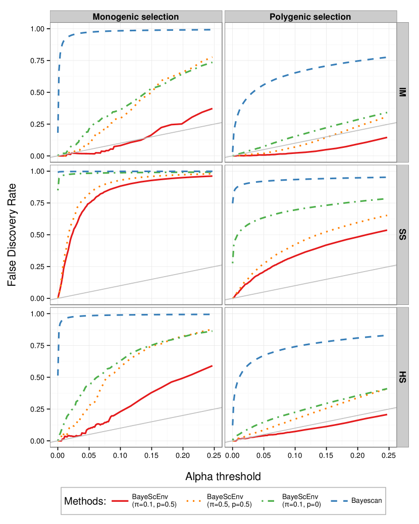
Figure 2: False Discovery Rate (FDR) against significance threshold $\alpha$ for three scenarios (IM: Island model, SS: Stepping-Stone model and HS: Hierarchically Structured model) and monogenic/polygenic selection. The grey line is the expected identity relationship between the FDR and $\alpha$. The models tested are BayeScan (blue dashed), and BayeScEnv (orange dotted, green dot-dashed and solid red) with different probabilities $\pi$ of jumping away from the neutral model (M1) and different preferences $p$ for the locus-specific model (M3). Note that $p=0$ means the environmental model (M2) is tested against the neutral one only.

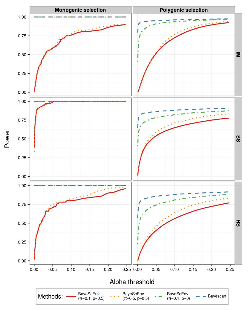
Figure 3: Power against significance threshold $\alpha$ for three scenarios (IM: Island model, SS: Stepping-Stone model and HS: Hierarchically Structured model) and monogenic/polygenic selection. The models tested are BayeScan (blue dashed), and BayeScEnv (orange dotted, green dot-dashed and solid red) with different probabilities $\pi$ of jumping away from the neutral model (M1) and different preferences $p$ for the locus-specific model (M3). Note that $p=0$ means the environmental model (M2) is tested against the neutral one only.

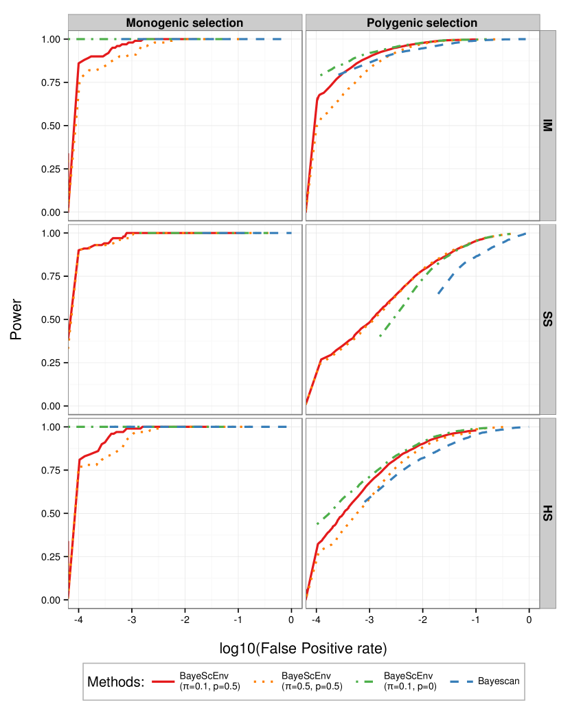
Figure 4: Power against False Positive Rate (FPR), a.k.a. ROC curve, for three scenarios (IM: Island model, SS: Stepping-Stone model and HS: Hierarchically Structured model) and monogenic/polygenic selection. The models tested are BayeScan (blue dashed), and BayeScEnv (orange dotted, green dot-dashed and solid red) with different probabilities $\pi$ of jumping away from the neutral model (M1) and different preferences $p$ for the locus-specific model (M3). Note that $p=0$ means the environmental model (M2) is tested against the neutral one only.

Results

Simulation results

By definition, a threshold value of $\alpha$ used to decide whether $q$-values are significant or not is expected to yield an FDR of $\alpha$ on the long run, when the model is robust and priors are calibrated.

As shown in Fig. 2, BayeScan was less well calibrated, yielding higher FDRs than BayeScEnv under all scenarios and for both monogenic and polygenic selection. Additionally, for BayeScEnv, the implementation using $\pi=0.1$ was fairly well calibrated (i.e. the curve is close the grey line in Fig. 2) under the IM scenario (for both monogenic and polygenic versions) and under the polygenic version of the HS scenario. This implementation was much more conservative than the one using $\pi=0.5$. For $\pi=0.1$ and $p=0$, the FDRs were closer to those yielded by BayeScan, but still lower.

The higher FDR for BayeScan and BayeScEnv with $\pi=0.5$ or $p=0$ was mainly driven by a higher FPR rather than a lack of power (Fig. 3, see also Fig. S3 in the SI). Notably though, BayeScan had a quite high power, higher than that of BayeScEnv. Note, however, that BayeScEnv with $p=0$ had, as BayeScan, a maximal power in the monogenic scenarios, and was almost as powerful as BayeScan in the polygenic scenarios. Yet its FDR was lower (sometimes much lower) than that of BayeScan. This indicates that the incorporation of environmental data helps to reduce the error rate both with or without the inclusion of spurious locus-specific effects ($\alpha_{i}$). More details regarding the FPR results are available in the Supplementary Information (Fig. S3).

Another traditional way to apprehend the compromise between power and false positives is the so-called ROC curve, plotting power against FPR (Fig. 4). In these plots, the curve that is “more to the left” is preferred because this means it offers higher power for a lower FPR. Fig. 4 shows that BayeScEnv with $\pi=0.1$ and $p=0$ performed best under the IM and HS scenarios, whereas BayeScEnv with $\pi=0.1$ and $p=0.5$ performed better under the “harder” SS scenario. Overall, although BayeScan has higher power to detect local adaptation, it is still too liberal when deciding that a locus is under selection for the scenarios we investigated.

Analysis of human data from Asia

The results of the human dataset analysis (Table 1) show a dramatic discrepancy between the two methods. Whereas BayeScan yields a very large number (66,316) of markers considered as significant at the 5% threshold, many fewer markers (154 to 2728) are considered significant by BayeScEnv. Gene Ontology (GO) enrichment tests identified many significant terms (Table 1). Note, however, that in the altitude and temperature analyses they correspond to a small number of genes (11 and 20 respectively, see Table 1). The number of genes is larger for the precipitation analysis (359) and even larger for the analysis using BayeScan (5628).

Regarding the altitude, significant biological processes included the fatty acid metabolism (e.g. SCARB1), skin pigmentation (e.g. MLANA, SLC24A5), kidney activity (e.g. SLC12A1) and oxido-reductase activity (e.g. NOS1AP ). Regarding the temperature, significant biological process included cardiac muscle activity (e.g. SLC8A1) and development (e.g. NRG1, FOXP1), fatty acid metabolism (e.g. FADS1, FADS2) and response to hypoxia (e.g. SLC8A1, SERPINA1). For the precipitation analysis with BayeScEnv, as well as the BayeScan analysis, the number of significant terms was too large for hand-picked examples to be feasible.

The significance results ($q$-values) are displayed as a Manhattan plot in Fig. 5, along with the above mentioned genes for the altitude and temperature analyses (Fig. 5, A and B). Other regions of the genome also include outlier loci but they correspond to non-coding regions, or are close to genes associated to GO terms that were not significant, or to proteins without a known function (e.g. C9orf91, which was the most significant gene in the temperature analysis). Pattern of linkage disequilibrium was visible, which sometimes strongly supported some candidate genes (Fig. 5, A, SLC12A1 and SLC24A5). Finally, comparing BayeScEnv (Fig. 5, A, B and C) and BayeScan analyses (Fig. 5,D), we see that BayeScan yielded too many significant markers for a Manhattan plot to be a useful display of the results. An interesting pattern is that BayeScan yielded far more outlier markers with maximal certainty (e.g. posterior probability of one) than BayeScEnv. For the present dataset, 22,516 markers had a posterior probability of one, whereas the maximal posterior probability yielded by BayeScEnv was 0.9998. Finally, almost all loci detected using BayeScEnv were also found when using BayeScan (between 98% for altitude to 100% for the two other variables).

Method	Variable	Nr of significant SNPs	Nr of significant GO terms	Nr of genes associated with a significant GO term
BayeScEnv	altitude	154	32	11
	temperature	170	103	20
	precipitation	2728	439	359
BayeScan	—	66,316	469	5628

Table 1: Results from BayeScan and BayeScEnv on the human dataset. FDR significance threshold was set to 5%. The total number of tested markers was 446,117.

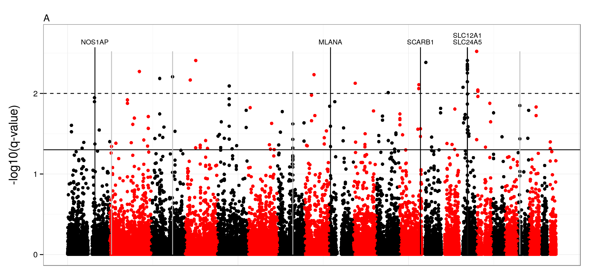
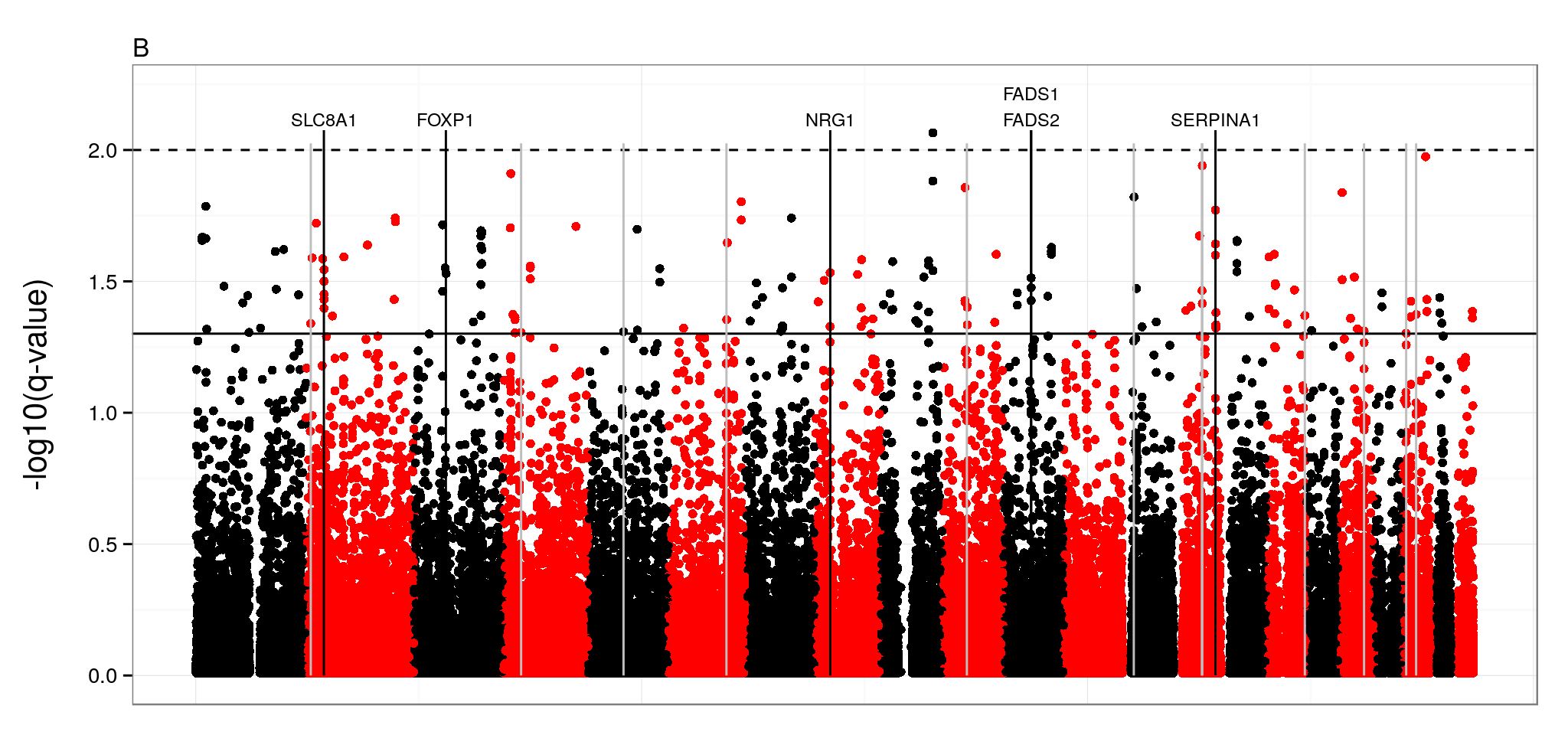
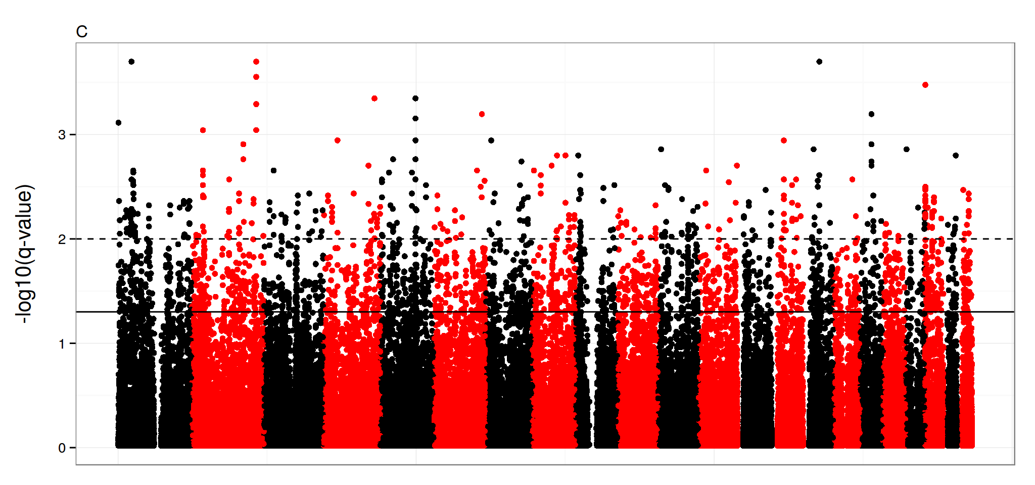
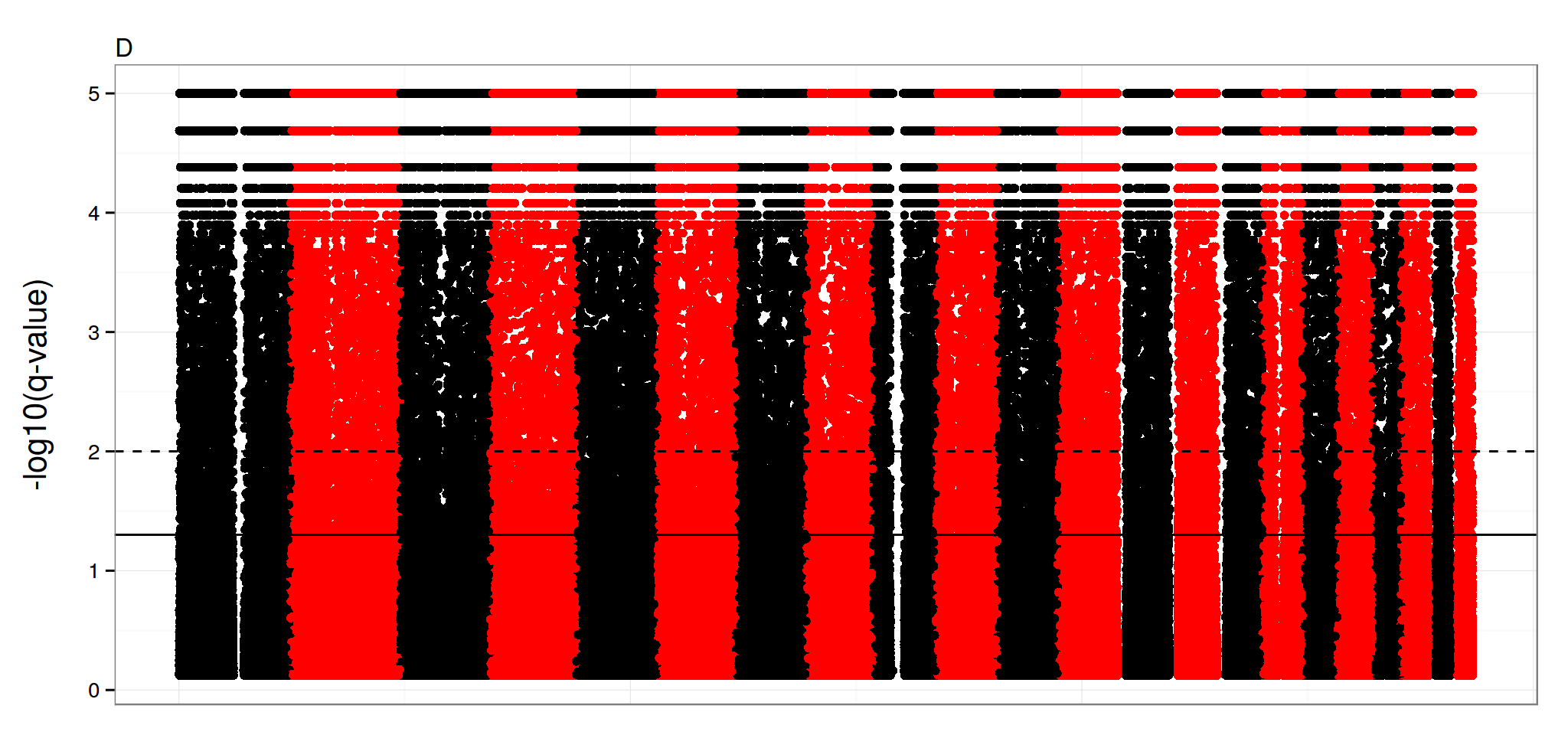
Figure 5: Manhattan plot of the $q$-values for the human dataset when using BayeScEnv with altitude (A), temperature (B), precipitations (C) or when using BayeScan (D). For altitude and temperature (A and B), genes mentioned in the text are displayed using black lines and genes associated with a significant GO term using grey lines. Top “stripes” for BayeScan (D) are artefacts due to finite number of iterations in RJMCMC (e.g. 0, 1, 2, 3… iterations outside of the non-neutral model), corresponding to determined posterior probabilities when divided by the total number of iterations.

Analysis of Atlantic salmon data

The results of the salmon dataset analyses (Table 2) are again a clear demonstration of the discrepancy between the methods. Whereas BayeScan yields 238 SNPs significant at the 5% level, BayeScEnv yields between 0 and 8 significant markers with $p=0.5$ and between 45 and 62 with $p=0$. Thus, in agreement with the theoretical expectations and the simulation studies, we obtain more candidates loci with $p=0$. All loci obtained when using BayeScEnv (for any variable and any value of $p$) were found when using BayeScan. Unfortunately, the Atlantic salmon genome is poorly annotated and, therefore, it was not possible to carry out a gene ontology enrichment analysis.

Method	Variable	Number of significant
		with $p=0.5$	with $p=0$
BayeScEnv	temperature	8	62
	precipitations	5	45
	river properties	0	46
BayeScan	—	238

Table 2: Results from the BayeScan and BayeScEnv on the salmon dataset. FDR significance threshold was set to 5%. The total number of tested markers was 2078.

Discussion

Features and performance of the method

The method we introduce in this paper, BayeScEnv, has several desirable features. First, just as BayeScan, it is a model-based method. This means that the null model can be understood in terms of a process of neutral evolution. One can thus predict what the method is able to fit or not. Second, we explicitly model a process of local adaptation caused by an environmental variable. Third, in order to render the model more robust, we account for locus-specific effects unrelated to the environmental variable under consideration. These departures can be due to another process of local adaptation (i.e. caused by unknown environmental variables), to large differences in mutation rates across loci, to background selection (Charlesworth, 2013) or complex spatial effects, such as allele surfing (Edmonds et al., 2004). Our simulation results show that when compared to BayeScan, BayeScEnv has a better control of its false discovery rate under various scenarios (Fig. 2), yielding fewer, but more reliable candidate markers. Obviously, this has a cost in terms of absolute power (Fig. 3), but BayeScEnv still performs better than BayeScan in terms of the compromise between true and false positives (Fig. 4).

Besides, the parametrisation of BayeScEnv allows for a fine and intuitive control of the false positive rate and power. For example, setting $p$ to 0 increases both power and false positive rate, whereas setting $p=0.5$ will allow for a more conservative test. This is because with $p=0$, thus in the absence of the locus-specific effect model (M3), the local adaptation model (M2) will absorb much of the signal in the data, yielding a higher probability of detecting true positives, but also a higher sensitivity to false positives. Our simulation results show that, if the species under study has moderate to large dispersal abilities (c.f. hierarchical structure or island model), the former parametrisation will be more appropriate, whereas for species with low dispersal abilities (c.f. stepping-stone model) the latter should be preferred. Thus, being able to choose the right parametrisation only requires limited knowledge about the dispersal abilities of the species.

We note that BayeScan was recently extended to consider species with hierarchical population structure (BayeScan3, Foll et al., 2014). With BayeScan3 it is now possible to study widely distributed species covering several continents or geographic regions. It is also possible to better focus on local adaptation by considering groups that include pairs of populations inhabiting different environments such as low and high altitude habitats. Thus, BayeScan3, allows for the consideration of categorical environmental variables. Our new approach on the other hand, allows the study of local adaptation related to continuous environmental variables in species with a more restricted range.

How to quantify ‘environmental differentiation’?

To model local adaptation, we compute an “environmental differentiation” in terms of the Manhattan distance to a reference value. Although this reference can conveniently be chosen as the average of the environmental values across the sampled populations, other kinds of reference may be biologically more relevant. For example, in our analysis of the effect of elevation in humans, it seems appropriate to use sea level as the reference. Indeed, given the kind of environmental variables elevation is a proxy for (e.g. partial pressure of oxygen, temperature, solar radiation, etc.), for most systems we would consider the sea level as a neutral environment rather than the differentiated one.

Another way to account for environmental differentiation is to use Principal Component Analysis (PCA), providing one of the axes to BayeScEnv as a description of the distance between environments. Despite this practice being an elegant way to summarise environmental distance between populations, it also has the drawback of making it more difficult to identify the “causal” variable.

Note that the environmental variables must be standardised so as to avoid scale inconsistencies between $g$ and $\alpha$ and $\beta$. If we choose the average environmental value as reference, then standardisation involves mean-centring and rescaling to have unit variance. However, if we choose another reference, then standardisation only involves rescaling to have unit variance.

Comparison with other environmental association methods

There are several genome-scan approaches that incorporate environmental information. Some are mechanistic (e.g. Bayenv, Coop et al., 2010) while others are phenomenological (e.g. LFMM, Frichot et al., 2013 and gINLAnd, Guillot et al., 2014). These methods perform a regression between allele frequencies and environmental values. Yet non-equilibrium situations combined with complex spatial structuring can lead to spatial correlations in allele frequencies, which in turn can lead to high false positive rates. To minimise this problem, the above methods take into account allele frequency correlations across populations while performing the regression.

BayeScEnv, on the other hand, assumes that all populations are independent, exchanging genes only through the migrant pool. However, it includes a locus-specific effect unrelated to the environmental variable that helps to take into account locus-specific spatial effects due to deviations from the underlying demographic model. The fact that this approach works is illustrated by our simulation study, which showed that BayeScEnv was fairly robust to isolation-by-distance and a hierarchically structured scenario. Moreover, the analyses of simulated datasets from de Villemereuil et al. (2014), available in the SI, show that even under very complex scenarios, BayeScEnv can compete with other environmental association methods. Nevertheless, we note that BayeScEnv is best suited for species with medium to high dispersal abilities such as marine species and anemophilous plants.

Another point that distinguishes BayeScEnv from these methods is that it does not assume any particular functional form for the relationship between environmental values and allele frequencies. While existing association methods all assume a clinal pattern, BayeScEnv only assumes that genetic differentiation increase exponentially with environmental differentiation. This allows for a more diverse family of relationships between allele frequencies and the environment. For example, a scenario where the same allele is favoured at the margins and counter selected in the middle of the species range can be studied with BayeScEnv but would certainly represent a problem for the other association methods. Such a scenario would arise, for instance, when the target of selection in extreme environments are plasticity genes (Morris et al., 2014), or genes regulating stress response. Alternatively, the chosen environmental variable might actually be a proxy for another selective variable that takes similar values when the former takes very low or very high values. For example, environments with very low or very high temperatures are often also arid environments. Another difficult scenario that BayeScEnv would be able to detect is one in which two populations with very similar values for the environmental factor have very different alleles frequencies at a locus and both experience environmental conditions very different from those of the other populations. Such patterns are difficult to relate to local adaptation and might most likely be caused by high drift in extreme environments, due to reduced population sizes. Yet, such a signal should in principle be captured by the $\beta$ parameter. One particular selective scenario that could explain such a pattern would be one of positive frequency-dependent selection modulated by the environment (i.e. only extreme environments would induce selection), as expected in the case of Mullerian mimicry with differential predator pressure (Borer et al., 2010). Nevertheless, the number of species where such a scenario would be biologically plausible is limited. In any case, loci showing such a pattern can be easily identified by post-hoc inspection of their allele frequencies in the different populations. It would then be possible to label these loci as false positives if frequency-dependent selection is deemed an unlikely scenario. All these scenarios are illustrated in the SI.

Finally, BayeScEnv is one of the very few methods to study gene-environment associations that can be used with dominant data (but see also Guillot et al., 2014).

Data analysis

When confronted with real datasets, BayeScEnv typically returned fewer significant markers than BayeScan. This is explained both by the focus on searching for outliers linked to a specific environmental factor and by the lower false positive rate of our approach. When applied to the human dataset, BayeScEnv identified several genomic regions that are enriched for gene ontology terms relevant to potential local adaptation to altitude or temperature. We emphasise that this study was not meant to exhaustively and rigorously investigate local adaptation in Asian human populations. However, our results tend to demonstrate that the candidates yielded by BayeScEnv have a biological interpretation. For example, skin pigmentation and cardiac activity could clearly be involved in responses to increased solar radiation and depleted oxygen availability at high elevation.

Much of the ontologies linked to temperature were potentially confounded with adaptation to altitude, such as the response to hypoxia and cardiac muscle activity. Also, fatty acid metabolism was associated to both altitude and temperature. Of course, the biological functions described here do not account for all the signals yielded by BayeScEnv (see Fig. 5, A and B). Other genomic significant regions include genes with less obvious biological function regarding local adaptation, non-coding regions and proteins without a known function. Finally, the analysis using the precipitation variable yielded too many significant markers for a detailed analysis of the biological functions involved. This may not necessarily be due to a confounding effect of the spatial structure (the human Asian populations being structured mainly from West to East, while the Eastern climate is characterised by strong precipitations during the monsoon), since precipitation may behave as a surrogate for several environmental variables.

As the Atlantic salmon genome is poorly annotated, we could not identify genes associated to the observed outlier loci. However, the discrepancy between the number of candidates yielded by BayeScan and BayeScEnv was still quite impressive in this case. Also, when using the parametrization $p=0$, we obtained almost an order of magnitude more candidates (though our simulations tend to demonstrate that this was probably at a cost of a larger false positive rate).

Conclusion

The main improvement introduced by our new method, BayeScEnv, over existing $F_{ST}$-based genome-scan approaches is the possibility of focusing on the detection of outlier loci linked to genomic regions involved in local adaptation and better distinguishing between the signal of positive selection and that of other locus-specific processes such as mutation and background selection. Although it does not explicitly model complex spatial effects, the consideration of two different locus-specific effects make it more robust to potential deviations from the migrant pool model. This is reflected in its much lower false discovery rate when compared to BayeScan.

Our new formulation also allows for an improved control of the true/false positives compromise through the parameter $p$, which describes our preference for the model that includes a locus-specific effect unrelated to the environmental factor over the model that includes environmental effects. Although we recommend using $p=0.5$, lower values (including 0) could be used if population structure is weak or maximising power is more important than reducing the false positive rate.

With this new method, there are now three alternative formulations of genome-scan methods based on the $F$ model. BayeScan detects a wide range of locus-specific effects (including background selection). Although its false discovery rate is higher than that of the two extensions, it is able to detect regions of the genome subject to purifying selection. The hierarchical version of this original formulation, BayeScan3, allows the study of local adaptation due to categorical environmental factors. Finally, our new method, BayeScEnv, is more appropriate to detect genomic regions under the influence of selective pressures exerted by continuous environmental variables. Thus, all three methods are complementary and jointly cover scenarios applicable to a wide range of species

Data Accessibility

The Python code used to simulate data is available online in the Supplementary Information. The software is available online at GitHub: http://github.com/devillemereuil/bayescenv.

Author contributions

PdV and OEG designed the statistical model. PdV modified the C++ code and performed the simulation and data analysis. PdV and OEG wrote the article.

Supplementary Information

1 Definition of the prior probabilities of jump between models

Recall the three models of which we want to infer posterior probabilities:

M1

Neutral model: $\log(\frac{1}{\theta_{ij}})=\beta_{j}$,

M2

Local adaptation model with environmental differentiation $\log(\frac{1}{\theta_{ij}})=\beta_{j}+g_{i}E_{j}$,

M3

Locus-specific model: $\log(\frac{1}{\theta_{ij}})=\alpha_{i}+\beta_{j}$.

Let $\Pi_{2}$ be the prior probability of model M2 and $\Pi_{3}$ the prior probability of model M3. We assume that the probability of going from M1 or M2 to the model M2 is equal to $\Pi_{2}$ (the same reasoning applies for M3 and $\Pi_{3}$), which leads to the following transition matrix:

$$\left(\begin{array}[]{ccc}1-\Pi_{2}-\Pi_{3}&\Pi_{2}&\Pi_{3}\\ (1-\Pi_{2})(1-\Pi_{3})&\Pi_{2}&\Pi_{3}(1-\Pi_{2})\\ (1-\Pi_{2})(1-\Pi_{3})&\Pi_{2}(1-\Pi_{3})&\Pi_{3}\end{array}\right).$$ (1)

If we consider $\Pi_{2}=\pi(1-p)$ and $\Pi_{3}=\pi p$ where $\pi$ is the probability of jumping away from model M1 and $p$ the “preference” for model M3 (i.e. the probability of choosing the model M3 instead of model M2, when jumping away from model M1), then we can write:

$$\left(\begin{array}[]{ccc}1-\pi&\pi(1-p)&\pi p\\ 1-\pi+\pi^{2}p(1-p)&\pi(1-p)&\pi p-\pi^{2}p(1-p)\\ 1-\pi+\pi^{2}p(1-p)&\pi(1-p)-\pi^{2}p(1-p)&\pi p\end{array}\right).$$ (2)

Thus, when $\pi$ is small (in practice $\pi<0.5$), the transition between models depends only very slightly on the current state of the model, and the prior probabilities of each model reduce approximately to (ignoring second order terms)

$$\begin{array}[]{rcl}P(\text{{M1}})&=&1-\pi,\\ P(\text{{M2}})&=&\pi(1-p),\\ P(\text{{M3}})&=&\pi p.\\ \end{array}$$ (3)

2 Reversible jumps between the models

According to Brooks (1998) and Gelman et al. (2004), the jump from model $l$ to model $k$ should be accepted with a probability $\text{min}(r,1)$, with

$$r=\frac{L(Y|\theta_{k},M_{k})P(\theta_{k}|M_{k})P(M_{k})}{L(Y|\theta_{l},M_{l})P(\theta_{l}|M_{l})P(M_{l})}\frac{J_{k\rightarrow l}J(u_{k}|\theta_{k},k,l)}{J_{l\rightarrow k}J(u_{l}|\theta_{l},l,k)}\left|\frac{\nabla g_{l,k}(\theta_{l},u)}{\nabla(\theta_{l},u)}\right|,$$ (4)

where $\theta_{\bullet}$ is the parameter vector for model $\bullet$, $L$ stands for the likelihood of parameters $\theta_{\bullet}$ assuming the model M${\bullet}$, and $J$ is the proposal kernel for the (potentially) new parameter $u_{\bullet}$. Note also the presence of the proposal of new model $J_{\circ\rightarrow\bullet}$.

Because a jump toward one of the two alternative models is proposed at each iterations, $\frac{J_{k\rightarrow l}}{J_{l\rightarrow k}}$ simplifies to one. Likewise, since the transformations from $\theta_{l}$ to $\theta_{k}$ only consists in setting some parameters to 0, the Jacobian determinant $\left|\frac{\nabla g_{l,k}(\theta_{l},u)}{\nabla(\theta_{l},u)}\right|$ also simplifies to one.

The most efficient way to propose a value for $u_{\bullet}$ is to draw from its own posterior (Brooks et al., 2003). Thus, pilot runs are carried out before the actual reversible jump MCMC in order to approximate the posteriors of $\alpha_{i}$ and $g_{i}$ for each locus $i$. During these runs, the parameters $\beta_{j}$ are inferred alone (M1 model), whereas the parameters $\alpha_{i}$ and $g_{i}$ are inferred using models containing $\beta_{j}$ (M2 and M3 models). The posterior mean and variance obtained for these parameters from the pilot runs are used to parametrise Normal distributions. These distributions are used to propose a new value of a parameter when a jump to a model including it is proposed. Note that, since $g_{i}$ cannot be negative, a truncated Normal is used, and the $J$ kernel is modified accordingly in Eq. 4.

3 Statistical tests

Using the posterior probability of model M2 for the locus $i$, $P_{i}(\text{{M2}}|\bm{a}_{i},E)$, we can calculate the posterior error probability (PEP, Käll et al., 2008) for locus $i$ as

$$\text{PEP}_{i}=1-P_{i}(\text{{M2}}|\bm{a}_{i},E).$$ (5)

In order to calculate the $q$-value (Storey, 2003; Muller et al., 2006), we rank the PEP_i from from the lowest to the highest value, and define the $q$-value for locus $i$ as the average PEP for all loci having a PEP lower, or equal to, PEP_i:

$$q_{i}=\frac{1}{i}\sum_{k,k\leq i}\text{PEP}_{k}.$$ (6)

Note that, because we calculate the average using only PEPs that are lower than PEP_i, we have $q_{i}\leq\text{PEP}_{i}$ for all $i$. The equality only holds for the minimal PEP(s). Käll et al. (2008) advocate the use of the $q$-value because it is optimal in the sense of Bayesian classification theory (see also Storey, 2003). Our code outputs both PEPs and $q$-values.
Both of these test statistics are strongly related to the control of False Discovery Rate (FDR, Storey, 2002) during multiple testing. Contrary to the commonly used False Positive Rate (FPR), which is the probability of declaring a locus as positive given that it is actually neutral, the FDR is the proportion of the positive results that are in fact false positives. Note that the PEP is a “locally” (i.e. regarding only the focal locus) inferred measure of the FDR (see Käll et al., 2008), whereas the $q$-value is based on inferring what the FDR would be when stating that the focal locus, and all the loci with a lower score should be considered as positives.
In the following, we will focus on the $q$-value of the local adaptation model (M2). Since we have a strong uncertainty regarding the biological origin of the locus-specific effect $\alpha_{i}$, we can consider it as a “nuisance” parameter in this particular inference framework.

4 Hierarchically Structured (HS) scenario

Fig. S1 gives a schematic representation of the demographic scenario called HS in the main text, showing the fission events and the migration between populations. Note that only some illustrative migration combinations are represented for the sake of simplicity. An important feature of this model is that the probability of migration between two populations decreases as their relatedness (measured by the number of fission events separating them) decreases. A full model description can be found in de Villemereuil et al. (2014).

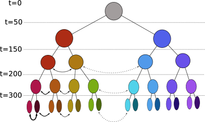
Figure S1: Schematic representation of the Hierarchically Structured scenario (HS). Fission events are shown as connectors and migration is denoted using double-arrow (thickness illustrate the strength of migration).

5 Simulation scripts

Four Python scripts are provided as Supplementary Files:

IM_mono.py

Island model with monogenic selection

IM_poly.py

Island model with polygenic selection

SS_poly.py

Stepping-stone model with polygenic selection

HS_poly.py

Hierarchically structured model with polygenic selection

These scripts require Python 2.7 and SimuPOP 1.1. Note that the monogenic version is provided only for the island model, as the modification are identical for the two other models.

6 Environmental gradient

The environmental gradient was designed to be independent from (i.e. not be confounded with) the population structure for the scenarios SS and HS (see Fig. S2).

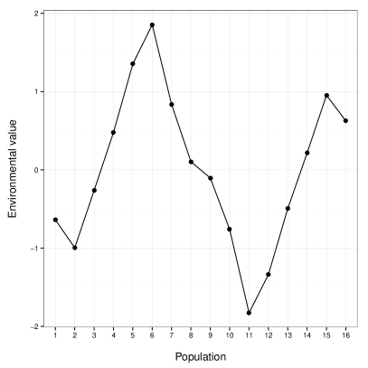
Figure S2: Environmental value for all 16 populations in the scenarios SS and HS.

This environmental variable was already standardised for its use in BayeScEnv. A transformation of this variable was used to define selective pressure on an appropriate scale:

$$s_{j}=s_{0}\frac{1-e^{-E_{j}}}{1+e^{-E_{j}}},$$ (7)

where $s_{0}$, the strength of the selection was chosen to be 0.1 for the monogenic case and 0.02 for the polygenic case. The individual fitness was calculated in a multiplicative fashion:

$$W=(1+s_{j})^{n_{11}}(1-s_{j})^{n_{00}},$$ (8)

where $n_{11}$ and $n_{00}$ are the number of loci at which the individual is homozygous for the advantageous and disadvantageous allele, respectively. Note that this fitness function assumes co-dominance, with a heterozygous fitness of 1.

The recombination rate was set to 0.002 (one recombination between two adjacent loci, per population and per generation). The mutation rate was set to $10^{-7}$ per generation at every locus. The allele frequencies were initialised using a beta-binomial distribution truncated between 0.1 and 0.9 to avoid too many monomorphic loci.

7 Simulation results for the False Positive Rate

The results regarding the False Positive Rate (FPR, Fig. S3) were qualitatively comparable to the results regarding the False Discovery Rate (FDR, Fig. 2, main text). Indeed, we again found that the most error-prone method was BayeScan, where BayeScEnv yielded fewer false positives. For the latter, the parametrisation $\pi=0.1$, $p=0.5$ was, as expected, the most conservative, whereas $\pi=0.1$, $p=0$ was the most laxist.

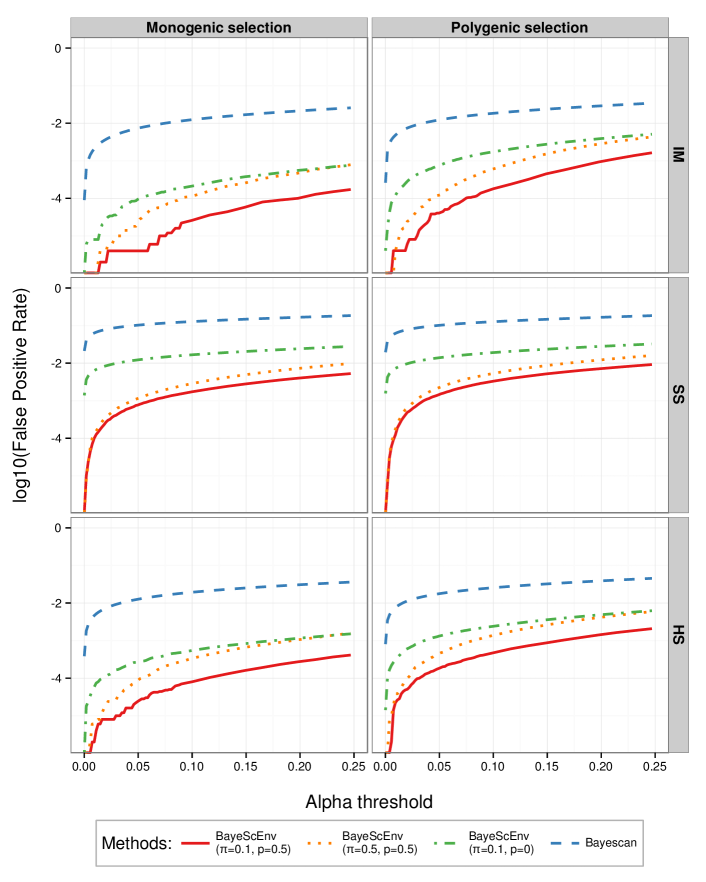
Figure S3: False Positive Rate (FPR) against significance threshold $\alpha$ for three scenarios (IM: Island model, SS: Stepping-Stone model and HS: Hierarchically Structured model) and monogenic/polygenic selection. The models tested are BayeScan (blue dashed), and BayeScEnv (orange dotted, green dot-dashed and solid red) with different probabilities $\pi$ of jumping away from the neutral model and different preferences $p$ for the locus-specific model. Note that $p=0$ means the environmental model is tested against the neutral one only.

8 List of candidate genes associated with significant GO terms

Below is a list of the genes that fulfill the following two criteria. First, there is at least one significant SNPs in their neighbourhood, indicating them as potential candidates for local adaptation. Second, at least one of their associated GO terms were found to be significantly enriched for candidates compared to the rest of the genome.

• For the altitude analysis: SCARB1, SLC12A1, MUCL1, DNM2, MLANA, ATP6V1C2, CLDN12, FBN1, OTUD7A, SLC24A5, NOS1AP, SLC12A8

• For the temperature analysis: SYNE2, SPTB, ANKRD46, HAO1, HCK, FOXP1, ONECUT2, CDH15, ATP8A2, FADS2, ESR2, ATP6V1C2, FADS1, NRG1, APBB2, CMYA5, SERPINA6, SLC8A1, PRKG1, LAMA2, SERPINA1

Note that the majority of the significant GO terms were represented by only one gene for the altitude and temperature analysis. The list of genes fulfilling the two criteria is not shown for the precipitation analysis and BayeScan, as there are too many of them.

9 Analysis of the simulation scenarios from de Villemereuil et al. (2014)

Scenarios

Given the computationally expensive nature of the simulations necessary to generate synthetic data, we compare BayeScEnv with methods other than BayeScan using the simulated datasets from de Villemereuil et al. (2014). For more information regarding these scenarios, please refer to the article. Briefly, four polygenic scenarios were tested:

HsIMM-C

Hierarchical scenario with a clinal environment following population structure

HsIMM-U

Hierarchical scenario with a random environment strongly correlated with population structure

IMM

Isolation with Migration Model

SS

Stepping-Stone model with a clinal environment, following the clinal population structure

Foreword

These scenarios were tested against BayeScan (Foll and Gaggiotti, 2008), Bayenv (Coop et al., 2010) and LFMM (Frichot et al., 2013). Note that these scenarios are very difficult for all methods, thus we do not expect the FDR to be well calibrated. Also, in contrast with the study in the main text, de Villemereuil et al. used a prior odds of 100 instead of 10 for BayeScan.
When interpreting the results, it should be remembered that the FDR depends on both the FPR and power. All things being equal, the FDR will be higher if the FPR is higher, and lower if the power is higher.

Results

The results are presented in Figs. S4–S6 (below). They show that, even under very difficult conditions, BayeScEnv inferences are fairly reliable. As expected, both the FPR and the power of BayeScEnv are lower than that of BayeScan, resulting in a more conservative method overall. However, in scenarios with low power for all methods, BayeScEnv’s lack of power can drastically inflate its FDR (e.g. Fig. S4, red line, IMM model). Interestingly, BayeScEnv with $p=0$ is more robust in this regard, since its power is generally much higher.
When compared to the other association methods (Bayenv and LFMM), BayeScEnv performed very well in “clinal” scenarios (HsIMM-C and SS), but more poorly in the other scenarios. However when considering the canonical $\alpha=0.05$ threshold, BayeScEnv’s FDR was always lower than at least one of the association methods, except in the IMM scenario.

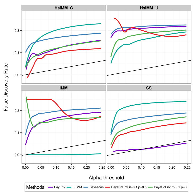
Figure S4: False Discovery Rate (FDR) against significance threshold $\alpha$ for de Villemereuil et al. (2014) polygenic scenarios.

False Discovery Rate

When comparing the FDR to other methods, BayeScEnv performs relatively well. Especially, for $p=0.5$ (red line), its FDR can be the lowest (HsIMM-C) or second best (SS), but it can reach very high values under some scenarios (HsIMM-U and IMM). Surprisingly, the parametrisation $p=0$ (green) is more stable across scenarios, whereas Bayenv (purple) and LFMM (turquoise) constantly “switch” between best-or-so and poorest-or-so. Overall, BayeScEnv’s FDRs with $p=0$ are lower than those of BayeScan’s, at least for the canonical threshold $\alpha=0.05$.

Large values of FDR for small $\alpha$’s are due to a lack of power (see below), not to a high False Positive Rate.

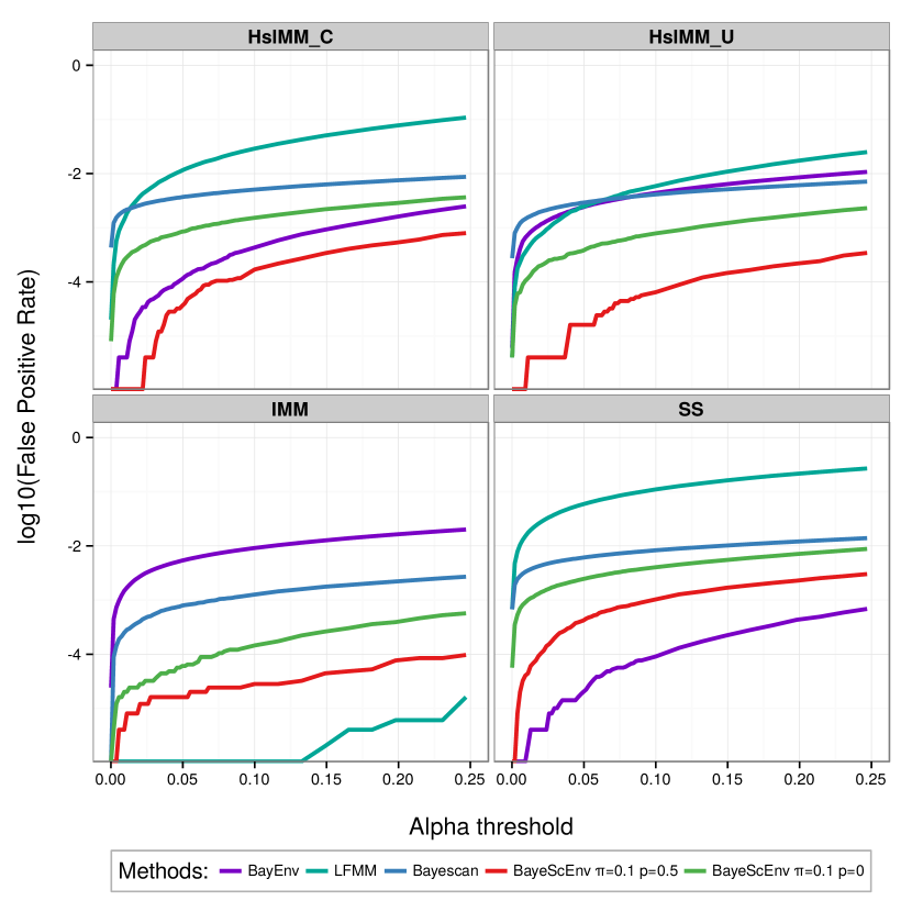
Figure S5: False Positive Rate (FPR) against significance threshold $\alpha$ for de Villemereuil et al. (2014) polygenic scenarios.

False Positive Rate

FPRs are more predictable than FDRs regarding the $F$ model family: BayeScan (blue) is the most error-prone method, followed by BayeScEnv with $p=0$ (green) while BayeScEnv with $p=0.5$ (red) is one of the most conservative methods. Interestingly, the FPRs of the $F$ model family are more stable than the FPRs of Bayenv (purple) and LFMM (turquoise), which vary greatly across scenarios.

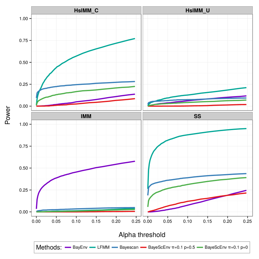
Figure S6: Power against significance threshold $\alpha$ for de Villemereuil et al. (2014) polygenic scenarios.

Power

Overall power varies greatly across scenarios, HsIMM-U and IMM being the most difficult ones. As expected, the power of BayeScEnv (red and green) is always lower than the power of BayeScan (blue). However, the power of BayeScEnv with $p=0$ (green), is always comparable to that of BayeScan’s. BayeScEnv with $p=0.5$ (red) is always among the less powerful method. For all scenarios, at least on of the environmental association methods (Bayenv (purple) and LFMM (turquoise)), has greater power than BayeScan and BayeScEnv.

10 Typical frequency patterns detected by BayeScEnv

Consider the standardised environmental variable $X_{j}$ from which we derived the environmental differentiation using $E_{j}=|X_{j}|$. As explained in the Discussion (see main text), we can distinguish three main patterns of population allele frequencies $f_{j}$ as a function of this environmental value $X_{j}$.

Clinal scenario
This is the canonical scenario, which was simulated in this study and most thoroughly investigated. It is also the scenario tested in all evaluations of environmental association methods.

“Plasticity” scenario
In this scenario, two populations with very different environmental values have similar allele frequencies. It could arise in situations where the environmental variable used is a proxy for a true environmental variable that has a non-monotonic relationship with the environmental variable used (e.g. very high or very low temperatures can both lead to aridity). More interestingly, it is expected, for example, from genes responsible for phenotypic plasticity (Morris et al., 2014).

Extreme frequencies scenario
In this scenario, populations with similar environmental values have extremely different allele frequencies. This scenario would lead to results that should in principle be interpreted as false positives. Note, however, that such a scenario could be explained by positive frequency-dependent selection triggered by the environmental variable.

References

- Akey et al. (2002) Akey JM, Zhang G, Zhang K, Jin L, Shriver MD (2002) Interrogating a high-density SNP map for signatures of natural selection. Genome Research, 12(12), 1805–1814.
- Beaumont and Balding (2004) Beaumont MA, Balding DJ (2004) Identifying adaptive genetic divergence among populations from genome scans. Molecular Ecology, 13(4), 969–980.
- Blanquart et al. (2013) Blanquart F, Kaltz O, Nuismer SL, Gandon S (2013) A practical guide to measuring local adaptation. Ecology Letters, 16(9), 1195–1205.
- Bonhomme et al. (2010) Bonhomme M, Chevalet C, Servin B, Boitard S, Abdallah J, Blott S, SanCristobal M (2010) Detecting selection in population trees: the Lewontin and Krakauer test extended. Genetics, 186(1), 241–262.
- Borer et al. (2010) Borer M, Van Noort T, Rahier M, Naisbit RE (2010) Positive frequency-dependent selection on warning color in Alpine leaf beetles. Evolution, 64(12), 3629–3633.
- Bourret et al. (2014) Bourret V, Dionne M, Bernatchez L (2014) Data from: Detecting genotypic changes associated with selective mortality at sea in Atlantic salmon: polygenic multi-locus analysis surpasses genome scan.
- Bourret et al. (2013a) Bourret V, Dionne M, Kent MP, Lien S, Bernatchez L (2013a) Landscape genomics in Atlantic salmon (Salmo salar): searching for gene–environment interactions driving local adaptation. Evolution, 67(12), 3469–3487.
- Bourret et al. (2013b) Bourret V, Kent MP, Primmer CR, Vasemägi A, Karlsson S, Hindar K, McGinnity P, Verspoor E, Bernatchez L, Lien S (2013b) SNP-array reveals genome-wide patterns of geographical and potential adaptive divergence across the natural range of Atlantic salmon (Salmo salar). Molecular Ecology, 22(3), 532–551.
- Brooks (1998) Brooks S (1998) Markov chain Monte Carlo method and its application. Journal of the Royal Statistical Society: Series D (The Statistician), 47(1), 69–100.
- Brooks et al. (2003) Brooks SP, Giudici P, Roberts GO (2003) Efficient construction of reversible jump Markov chain Monte Carlo proposal distributions. Journal of the Royal Statistical Society: Series B (Statistical Methodology), 65(1), 3–39.
- Charlesworth (1998) Charlesworth B (1998) Measures of divergence between populations and the effect of forces that reduce variability. Molecular Biology and Evolution, 15(5), 538–543.
- Charlesworth (2013) Charlesworth B (2013) Background selection 20 years on: The Wilhelmine E. Key 2012 Invitational Lecture. Journal of Heredity, 104(2), 161–171.
- Coop et al. (2010) Coop G, Witonsky D, Di Rienzo A, Pritchard JK (2010) Using environmental correlations to identify loci underlying local adaptation. Genetics, 185(4), 1411–1423.
- De Mita et al. (2013) De Mita S, Thuillet AC, Gay L, Ahmadi N, Manel S, Ronfort J, Vigouroux Y (2013) Detecting selection along environmental gradients: analysis of eight methods and their effectiveness for outbreeding and selfing populations. Molecular Ecology, 22(5), 1383–1399.
- Duforet-Frebourg et al. (2014) Duforet-Frebourg N, Bazin E, Blum MGB (2014) Genome scans for detecting footprints of local adaptation using a bayesian factor model. Molecular Biology and Evolution, 31(9), 394–407.
- Edelaar et al. (2011) Edelaar P, Burraco P, Gomez-Mestre I (2011) Comparisons between Qst and Fst—how wrong have we been? Molecular Ecology, 20(23), 4830–4839.
- Edmonds et al. (2004) Edmonds CA, Lillie AS, Cavalli-Sforza LL (2004) Mutations arising in the wave front of an expanding population. Proceedings of the National Academy of Sciences of the United States of America, 101(4), 975–979.
- Faria et al. (2014) Faria R, Renaut S, Galindo J, Pinho C, Melo-Ferreira J, Melo M, Jones F, Salzburger W, Schluter D, Butlin R (2014) Advances in ecological speciation: an integrative approach. Molecular Ecology, 23(3), 513–521.
- Foll and Gaggiotti (2008) Foll M, Gaggiotti OE (2008) A genome-scan method to identify selected loci appropriate for both dominant and codominant markers: A Bayesian perspective. Genetics, 180(2), 977 –993.
- Foll et al. (2014) Foll M, Gaggiotti OE, Daub JT, Vatsiou A, Excoffier L (2014) Widespread signals of convergent adaptation to high altitude in Asia and America. The American Journal of Human Genetics, 95(4).
- Frichot et al. (2013) Frichot E, Schoville SD, Bouchard G, François O (2013) Testing for associations between loci and environmental gradients using latent factor mixed models. Molecular Biology and Evolution, 30(7), 1687–1699.
- Gaggiotti and Foll (2010) Gaggiotti OE, Foll M (2010) Quantifying population structure using the F-model. Molecular Ecology Resources, 10(5), 821–830.
- Gelman et al. (2004) Gelman A, Carlin JB, Stern HS, Rubin DB (2004) Bayesian data analysis. Text in Statisctical Science. Chapman & Hall/CRC Press, Boca Raton, Florida (US), second edition.
- Green (1995) Green PJ (1995) Reversible jump Markov chain Monte Carlo computation and Bayesian model determination. Biometrika, 82(4), 711–732.
- Guillot et al. (2014) Guillot G, Vitalis R, Rouzic Al, Gautier M (2014) Detecting correlation between allele frequencies and environmental variables as a signature of selection. A fast computational approach for genome-wide studies. Spatial Statistics, 8, 145–155.
- Günther and Coop (2013) Günther T, Coop G (2013) Robust identification of local adaptation from allele frequencies. Genetics, 195(1), 205–220.
- Kofler and Schlötterer (2012) Kofler R, Schlötterer C (2012) Gowinda: unbiased analysis of gene set enrichment for genome-wide association studies. Bioinformatics, 28(15), 2084–2085.
- Kruuk et al. (1999) Kruuk LEB, Baird SJE, Gale KS, Barton NH (1999) A comparison of multilocus clines maintained by environmental adaptation or by selection against hybrids. Genetics, 153(4), 1959–1971.
- Käll et al. (2008) Käll L, Storey JD, MacCoss MJ, Noble WS (2008) Posterior error probabilities and false discovery rates: Two sides of the same coin. Journal of Proteome Research, 7(1), 40–44.
- Luikart et al. (2003) Luikart G, England PR, Tallmon D, Jordan S, Taberlet P (2003) The power and promise of population genomics: from genotyping to genome typing. Nature Reviews Genetics, 4(12), 981–994.
- Morris et al. (2014) Morris MRJ, Richard R, Leder EH, Barrett RDH, Aubin-Horth N, Rogers SM (2014) Gene expression plasticity evolves in response to colonization of freshwater lakes in threespine stickleback. Molecular Ecology, 23(13), 3226–3240.
- Muller et al. (2006) Muller P, Parmigiani G, Rice K (2006) FDR and bayesian multiple comparisons rules. Johns Hopkins University, Dept. of Biostatistics Working Papers.
- Nicholson et al. (2002) Nicholson G, Smith AV, Jónsson F, Gústafsson O, Stefánsson K, Donnelly P (2002) Assessing population differentiation and isolation from single-nucleotide polymorphism data. Journal of the Royal Statistical Society. Series B (Statistical Methodology), 64(4), 695–715.
- Peng and Kimmel (2005) Peng B, Kimmel M (2005) simuPOP: a forward-time population genetics simulation environment. Bioinformatics, 21(18), 3686–3687.
- Riebler et al. (2008) Riebler A, Held L, Stephan W (2008) Bayesian variable selection for detecting adaptive genomic differences among populations. Genetics, 178(3), 1817–1829.
- Shendure and Ji (2008) Shendure J, Ji H (2008) Next-generation DNA sequencing. Nature Biotechnology, 26(10), 1135–1145.
- Storey (2002) Storey JD (2002) A direct approach to false discovery rates. Journal of the Royal Statistical Society: Series B (Statistical Methodology), 64(3), 479–498.
- Storey (2003) Storey JD (2003) The positive false discovery rate: A Bayesian interpretation and the q-value. Annals of Statistics, pp. 2013–2035.
- de Villemereuil et al. (2014) de Villemereuil P, Frichot E, Bazin E, François O, Gaggiotti OE (2014) Genome scan methods against more complex models: when and how much should we trust them? Molecular Ecology, 23(8), 2006–2019.