Language Edit Distance & Maximum Likelihood Parsing of Stochastic Grammars: Faster Algorithms & Connection to Fundamental Graph Problems

Abstract

Given a context free language $\mathcal{L(G)}$ over alphabet $\Sigma$ and a string $s\in\Sigma^{*}$, the language edit distance problem seeks the minimum number of edits (insertions, deletions and substitutions) required to convert $s$ into a valid member of $\mathcal{L(G)}$. The well-known dynamic programming algorithm solves this problem in $O(n^{3})$ time (ignoring grammar size) where $n$ is the string length [Aho, Peterson 1972, Myers 1985]. Despite its numerous applications, to date there exists no algorithm that computes exact or approximate language edit distance problem in true subcubic time.

In this paper we give the first such algorithm that computes language edit distance almost optimally. For any arbitrary $\epsilon>0$, our algorithm runs in $\tilde{O}(\frac{n^{\omega}}{poly(\epsilon)})$ time and returns an estimate within a multiplicative approximation factor of $(1+\epsilon)$ with high probability, where $\omega$ is the exponent of ordinary matrix multiplication of $n$ dimensional square matrices. It also computes the edit script. We further solve the local alignment problem; for all substrings of $s$, we can estimate their language edit distance within $(1\pm\epsilon)$ factor in $\tilde{O}(\frac{n^{\omega}}{poly(\epsilon)})$ time with high probability. Next, we design the very first subcubic ($\tilde{O}(n^{\omega})$) algorithm that given an arbitrary stochastic context free grammar, and a string returns the maximum likelihood parsing of that string. Stochastic context free grammars significantly generalize hidden Markov models; they lie at the foundation of statistical natural language processing, and have found widespread applications in many other fields.

To complement our upper bound result, we show that exact computation of maximum likelihood parsing of stochastic grammars or language edit distance with insertion-only edits in true subcubic time will imply a truly subcubic algorithm for all-pairs shortest paths, a long-standing open question. This will result in a breakthrough for a large range of problems in graphs and matrices due to subcubic equivalence. By a known lower bound result [Lee 2002], even the much simpler problem of parsing a context free grammar is as hard as boolean matrix multiplication. Therefore any nontrivial multiplicative approximation algorithms for either of the two problems in time $o(n^{\omega})$ are unlikely to exist.

1 Introduction

Given a model for data semantics and structures, estimating how well a dataset fits the model is a core question in large-scale data analysis. Formal languages (e.g., regular language, context free language) provide a generic technique for data modeling. The deviation from a model is measured by the least changes required in data to perfectly fit the model. Aho and Peterson studied this basic question more than forty years back to design error-correcting parsers for programming languages. Given a context free grammar (CFG) ${\mathcal{L}}(G)$ over alphabet $\Sigma$ and a string $s\in\Sigma^{*}$, they proposed the language edit distance problem, which determines the fewest number of edits (insertions, deletions and substitutions) along with an edit script to convert $s$ into a valid member of ${\mathcal{L}}(G)$. Due to its fundamental nature, the language edit distance problem has found many applications in compiler optimization (error-correcting parser [3, 30]), data mining and data management (anomaly detection, mining and repairing data quality problems [22, 16, 33]), computational biology (biological structure prediction [18, 42]), machine learning (learning topic and behavioral models [20, 29, 35]), and signal processing (video and speech analysis [43]).

Often it is natural to consider a probabilistic generative model, and ask for the most probable derivation/explanation of the observed data according to the model. Stochastic context free grammar (SCFG) is an example of that. It associates a conditional probability to each production rule of a CFG (see definition in Section 1.2) which reflects the likelihood of applying it to generate members of the language. SCFGs significantly generalize hidden Markov model, and several stochastic processes such as Latent Dirichlet Allocation [20] and Galton-Watson branching process [28]. They lie at the foundation of statistical natural language processing, and have found wide-spread applications as a rich framework for modeling complex phenomena [19, 49, 39, 14]. The most probable derivation of a string according to a stochastic context free grammar is known as the maximum likelihood parsing of SCFG, or simply as SCFG parsing.

The well-known Cocke-Younger-Kasami (CYK) algorithm for context free grammar parsing can be easily modified to solve the SCFG parsing problem in $O(|G|n^{3})$ time, where $|G|$ is the grammar size and $n$ is the length of the input sequence. After half a century since the proposal of CYK algorithm, there still does not exist a “true” subcubic algorithm for SCFG parsing that runs in $O(n^{3-\gamma})$ time in the string length for some $\gamma>0$. For the language edit distance problem, the proposed algorithm by Aho and Peterson has a running time of $O(|G|^{2}n^{3})$ [3]. The dependency on grammar size in run time was later improved by Myers to $O(|G|n^{3})$ [30]. Naturally, the cubic time-complexity on string length is a major bottleneck for most applications. Except minor polylogarithmic improvements over $O(n^{3})$ [42, 34, 48], till date true subcubic algorithms for the language edit distance problem, or the SCFG parsing have not been found.

In this paper, we make several contributions.

Upper Bound.

1. We give the first true subcubic algorithm to approximate language edit distance for arbitrary context free languages almost optimally. Our algorithm runs in $\tilde{O}(|G|^{2}\frac{n^{\omega}}{poly(\epsilon)})$ time and computes the language edit distance within a multiplicative approximation factor of $(1+\epsilon)$ for any $\epsilon>0$, where $\omega$ is the exponent of ordinary matrix multiplication over $(\times,+)$-ring [25] (Section 2). Therefore, if $d$ is the optimum distance, the computed distance is in $[d,d(1+\epsilon)]$. The best known bound for $\omega<2.373$ [45]. In fact the running time can be further improved to $\tilde{O}\bigg{(}\frac{1}{poly(\epsilon)}\Big{(}|G|n^{\omega}+\omega(n|G|,n,n|G|)+|G|^{2}n^{2}\Big{)}\bigg{)}$ where $\omega(n|G|,n,n|G|)$ is the running time of fast rectangular matrix multiplication of a $n|G|\times n$ matrix with a $n\times n|G|$ matrix. The algorithm also computes an edit script.

The above result is obtained by casting the problem as an algebraic closure computation problem [2]. All-pairs shortest path problem, and many other variants of path problems on graphs can be viewed as computing closure over an algebra which is a semiring. However, for the language edit distance computation, the underlying algebra is not a semiring; the corresponding “multiplication” operation is neither commutative, nor associative. This poses significant difficulties, and requires new techniques. Being more generic, our approximation algorithm can be employed to obtain alternate approximation schemes for a large variety of problems such as all-pairs shortest paths, minimum weight triangle/cycle detection, computing diameter, radius and many others in $\tilde{O}(m^{\omega}\log{W})$ time over $m$-node graphs where $W$ is the maximum absolute weight of any edge.

We note that by a lower bound result of Lee [26], it is known that a faster context free grammar parsing (distinguishing between $0$ and nonzero edit distance) leads to a faster algorithm for boolean matrix multiplication. Therefore, obtaining any multiplicative approximation factor for language edit distance in $o(n^{\omega})$ time is unlikely.

Our algorithm also solves the local alignment problem where given ${\mathcal{L}}(G)$ and $\sigma\in\Sigma^{*}$, for all substrings $\sigma^{\prime}$ of $\sigma$, we need to compute their language edit distance (Section 2). Such local alignment problems are studied extensively under string edit distance computation for approximate pattern matching, for the simpler problem of context free parsing etc. [1, 17]. Since, there are $\Theta(n^{2})$ different substrings and at least linear time per substring is required to return an edit script, $\Theta(n^{3})$ time is unavoidable for reporting all edit scripts. Our algorithm runs in $\tilde{O}(|G|^{2}\frac{n^{\omega}}{poly(\epsilon)})$ time, and provides an $(1\pm\epsilon)$-approximation for the local alignment problem with high probability ( prob $>1-\frac{1}{n}$). In addition, for any substring $\sigma^{\prime}$, of size $k$ , the corresponding edit script can be computed in an additional $O(k)$ time.

1. We design the first subcubic algorithm for SCFG parsing near-optimally (Section 3). Given a SCFG, which is a pair of CFG and a probability assignment on each production, $(G,{\bf{p}})$, and a string $s$, $|s|=n$, we give an $\tilde{O}(|G|^{2}n^{\omega}\log{\log{\frac{1}{p_{min}}}})$ algorithm to compute a parse $\pi^{\prime}(s)$ such that

   $|\log{{\sf Pr}\left[\pi^{\prime}(s)\right]}|\geq(1-\epsilon)|\log{{\sf Pr}\left[\pi(s)\right]}|$

   where $\pi(s)$ is the most likely parse of $s$ with the highest probability ${\sf Pr}\left[\pi(s)\right]$, and $p_{min}$ is the minimum probability of any production. To the best of our knowledge, prior to our work, no true subcubic algorithm for arbitrary SCFG parsing was known.

Lower Bound. In a pursuit to explain the difficulty in obtaining exact subcubic algorithms, we show that a subcubic algorithm for SCFG parsing or computing language edit distance (with only insertion) will culminate in a breakthrough result for several fundamental graph problems. In particular, we show any subcubic algorithm for the SCFG parsing leads to a subcubic algorithm for the all-pairs shortest paths problem (APSP). Similarly, if language edit distance where only insertion is allowed as edit operation has a subcubic algorithm, so does APSP. This establishes surprising connection to these problems with a fundamental graph problem for which obtaining a subcubic algorithm is a long-standing open question.

Theorem 1.

Given a stochastic context-free grammar $\{G=({\mathcal{N}},\Sigma,{\mathcal{P}},S),{\bf p}\}$, and a string $s\in\Sigma^{*}$, $|s|=n$, if the SCFG parsing problem can be solved in $O(|G|n^{3-\delta}\max{\log_{p\in\bf{p}}\frac{1}{p}})$ time then that implies an algorithm with running time $\tilde{O}(m^{3-\delta/3}\log{W})$ for all-pairs shortest path problem on weighted digraphs with $m$ vertices and maximum weight $W$.

Theorem 2.

Given a context-free grammar $G$, and a string $s\in\Sigma^{*}$, $|s|=n$, if the language edit distance problem with only insertion as allowable edit can be solved in $O(|G|n^{3-\delta})$ time then that implies an $\tilde{O}(m^{3-\delta/3}\log{W})$ algorithm for all-pairs shortest path problem on weighted digraphs with $m$ vertices and maximum edge weight $W$.

Our lower bound results build upon a construction given by Lee [26] who showed a faster algorithm for CFG parsing implies a faster algorithm for boolean matrix multiplication. For SCFG parsing, by suitably modifying his construction, we show a subcubic SCFG parser implies a subcubic $(\min,\times)$ matrix product computation . Next, we prove a subcubic algorithm for $(\min,\times)$ matrix product leads to a subcubic algorithm for negative triangle detection in weighted graphs. Negative triangle detection is one of the many problems known to be subcubic equivalent with all-pairs shortest path problem [46]. Our second reduction interestingly also shows computing $(\min,+)$ product of matrices with real weights bounded by $\log{n}$ in subcubic time is unlikely to exist. In contrast, $(\min,+)$ product of matrices with integer weights bounded by $\log{n}$ can be done fast in $O(n^{\omega}\log{n})$ time. Our lower bound result for language edit distance also uses similar construction and builds upon it to additionally handle edit distance.

By subcubic equivalence [46, 1], a subcubic algorithm for language edit distance or SCFG parsing implies a subcubic algorithm for a large number of graph problems, e.g. detecting minimum weight triangle, minimum weight cycle, checking metricity, finding second shortest path, replacement path, radius problem.

Corollary 1.

Given a stochastic context-free grammar $\{G=({\mathcal{N}},\Sigma,{\mathcal{P}},S),{\bf p}\}$, and a string $s\in\Sigma^{*}$, $|s|=n$, if the SCFG parsing problem can be solved in $O(|G|n^{3-\delta}\max{\log_{p\in\bf{p}}\frac{1}{p}})$ time then that implies an algorithm with running time $\tilde{O}(m^{3-\delta/3})$, $\gamma,\delta>0$ for all of the following problems.

1. Minimum weight triangle: Given an $n$-node graph with real edge weights, compute $u,v,w$ such that $(u,v),(v,w),(w,u)$ are edges and the sum of edge weights is minimized.

2. Negative weight triangle: Given an $n$-node graph with real edge weights, compute $u,v,w$ such that $(u,v),(v,w),(w,u)$ are edges and the sum of edge weights is negative.

3. Metricity: Determine whether an $n\times n$ matrix over $\mathbb{R}$ defines a metric space on $n$ points.

4. Minimum cycle: Given an $n$-node graph with real positive edge weights, find a cycle of minimum total edge weight.

5. Second shortest paths: Given an $n$-node directed graph with real positive edge weights and two nodes $s$ and $t$, determine the second shortest simple path from $s$ to $t$.

6. Replacement paths: Given an $n$-node directed graph with real positive edge weights and a shortest path $P$ from node $s$ to node $t$, determine for each edge $e\in P$ the shortest path from $s$ to $t$ in the graph with $e$ removed.

7. Radius problem: Given an $n$-node weighted graph with real positive edge weights, determine the minimum distance $r$ such that there is a vertex $v$ with all other vertices within distance $r$ from $v$.

Language edit distance computation is much harder than language recognition (or parsing). A beautiful result by Valiant was the first to overcome the barrier of cubic running time for context free recognition, and provided an $\tilde{O}(|G|^{2}n^{\omega})$ algorithm [41]. Our result surprisingly indicates that parsing time is enough to compute a near-optimal result for the much harder language edit distance problem. Is this result generally true? Our prior work on Dyck language edit distance obtained a polylogarithmic approximation guarantee in near parsing time (linear time for Dyck language) [37]. The Dyck language edit distance significantly generalizes string edit distance problem. Hence, a better than poly-log approximation guarantee in parsing time for Dyck language edit distance will also lead to improved approximation factor for string edit distance computation in near-linear time. Understanding the relation between parsing time, and language edit distance computation remains a big challenge.

Our current algorithm due to its algebraic nature is not practical. Obtaining a combinatorial subcubic algorithm remains a major open problem. Improving the dependency on $\frac{1}{\epsilon}$ will be important.

Grammars are a versatile method to encode problem structures. Lower bounds with grammar based distance computation may shed light into deriving unconditional lower bounds for polynomial time solvable problems, for which our understandings are still lacking.

1.1 Related Works

The language edit distance problem is a significant generalization of the widely-studied string edit distance problem where two strings need to be matched with minimum number of edits. The string edit distance problem can be exactly computed in quadratic time. Despite many efforts, a sub-quadratic exact algorithm for string edit distance does not exist. A recent result by Backurs and Indyk explains this difficulty by showing a sub-quadratic algorithm for string edit distance implies sub-exponential algorithm for satisfiability [9]. Our lower bound results are in a similar spirit which connects subcubic algorithm for language edit distance, and SCFG parsing to graph problems for which obtaining exact subcubic algorithms are long-standing open questions. For approximate string edit distance computation, there is a series of works that tried to lower the running time to near-linear [38, 13, 24, 10, 11, 8, 7].

Language recognition and parsing problems have been studied for variety of languages under different models for decades [27, 12, 23, 6, 32]. The works of [27, 12, 23] study the complexity of recognizing Dyck language in space-restricted streaming model. Alon, Krivelevich, Newman and Szegedy consider testing regular language and Dyck language recognition problem using sub-linear queries [6], followed by improved bounds in works of [32]. The early works of $O(n^{3})$ time algorithm for parsing context free grammars (such as the Cocke-Younger-Kasami algorithm (CYK or CKY algorihtm)) was improved by an elegant work of Valiant who obtained the first subcubic algorithm for context free grammar parsing [41]. For stochastic grammar parsing and language edit distance computation, till date there does not exist any true subcubic algorithm, except for minor polylogarithmic improvements in the running time [42, 34, 48].

1.2 Preliminaries

Grammars & Derivations. A context-free grammar (grammar for short) is a $4$-tuple $G=({\mathcal{N}},\Sigma,{\mathcal{P}},S)$ where ${\mathcal{N}}$ and $\Sigma$ are finite disjoint collection of nonterminals and terminals respectively. ${\mathcal{P}}$ is the set of productions of the form $A\rightarrow\alpha$ where $A\in{\mathcal{N}}$ and $\alpha\in({\mathcal{N}}\cup\Sigma)^{*}$. $S$ is a distinguished start symbol in ${\mathcal{N}}$.

For two strings $\alpha,\beta\in({\mathcal{N}}\cup\Sigma)^{*}$, we say $\alpha$ directly derives $\beta$, written as $\alpha\Rightarrow\beta$, if one can write $\alpha=\alpha_{1}A\alpha_{2}$ and $\beta=\alpha_{1}\gamma\alpha_{2}$ such that $A\rightarrow\gamma\in{\mathcal{P}}$. Thus, $\beta$ is a result of applying the production $A\rightarrow\gamma$ to $\alpha$.

${\mathcal{L}}(G)$ is the context-free language generated by grammar $G$, i.e., ${\mathcal{L}}(G)=\{w\in\Sigma^{*}\mid S\xRightarrow{\ast}w\}$, where $\xRightarrow{\ast}$ implies that $w$ can be derived from $S$ using one or more production rules. If we always first expand the leftmost nonterminal during derivation, we have a leftmost derivation. Similarly, one can have a rightmost derivation. If $s\in{\mathcal{L}}(G)$ it is always possible to have a leftmost (rightmost) derivation of $s$ from $S$.

We only consider grammars for which all the nonterminals are reachable, that is each of them is included in at least one derivation of a string in the language from $S$. Any unreachable nonterminal can be easily detected and removed decreasing the grammar size.

Chomsky Normal Form (CNF). We consider the CNF representation of $G$. This implies every production is either of type (i) $A\rightarrow BC$,  $A,B,C\in{\mathcal{N}}$, or (ii) $A\rightarrow x,~{}x\in\Sigma$ or (iii) $S\rightarrow\varepsilon$ if $\varepsilon\in{\mathcal{L}}(G)$. It is well-known that every context-free grammar has a CNF representation. CNF representation is popularly used in many algorithms, including CYK and Earley’s algorithm for CFG parsing [21]. Prior works on cubic algorithms for language edit distance computation use CNF representation as well [3, 30]

Definition 1 (Language Edit Distance).

Given a grammar $G=({\mathcal{N}},\Sigma,{\mathcal{P}},S)$ and $s\in\Sigma^{*}$, the language edit distance between $G$ and $s$ is defined as $d_{G}(G,s)=\min_{z:\in{\mathcal{L}}(G)}\mathrm{d}_{ed}(s,z)$ where $\mathrm{d}_{ed}$ is the standard edit distance (insertion, deletion and substitution) between $s$ and $z$. If this minimum is attained by considering $z\in{\mathcal{L}}(G)$, then $z$ serves as an witness for $\mathrm{d}_{G}(G,s)$.

We will often omit the subscript from $\mathrm{d}_{G}$ and $\mathrm{d}_{ed}$ and use $\mathrm{d}$ to represent both language and string edit distance when that is clear from the context. We assume ${\mathcal{L}}(G)\neq\phi$ and $\varepsilon\in{\mathcal{L}}(G)$ so that $\mathrm{d}_{G}(G,s)\leq|s|$.

Definition 2 ($t$-approximation for Language Edit Distance).

Given a grammar $G=({\mathcal{N}},\Sigma,{\mathcal{P}},S)$ and $s\in\Sigma^{*}$, a $t$-approximation algorithm for language edit distance problem, $t\geq 1$, returns a string $s^{\prime}$ such that $s^{\prime}\in{\mathcal{L}}(G)$ and $\mathrm{d}_{G}(G,s)\leq\mathrm{d}_{ed}(s^{\prime},s)\leq t*\mathrm{d}_{G}(G,s)$.

Definition 3.

A stochastic context free grammar (SCFG) is a pair $(G,{\bf p})$ where

• $G=({\mathcal{N}},\Sigma,{\mathcal{P}},S)$ is a context free grammar, and

• we additionally have a parameter $p(\alpha\rightarrow\beta)$ where $\alpha\in{\mathcal{N}},\alpha\rightarrow\beta\in{\mathcal{P}}$ for every production in ${\mathcal{P}}$ such that

  • $p(\alpha\rightarrow\beta)>0$ for all $\alpha\rightarrow\beta\in{\mathcal{P}}$

  • $\sum_{\alpha\rightarrow\beta\in{\mathcal{P}}:\alpha=X}p(\alpha\rightarrow\beta)=1$ for all $X\in{\mathcal{N}}$

  $p(\alpha\rightarrow\beta)$ can be seen as the conditional probability of applying the rule $\alpha\rightarrow\beta$ given that the current nonterminal being expanded in a derivation is $\alpha$.

Given a string $s\in\Sigma^{*}$ and a parse $\pi(s)$ where $\pi$ applies the productions $P_{1}P_{2}...P_{l}$ successively to derive $s$, probability of $\pi(s)$ under SCFG is

$${\sf Pr}\left[\pi(s)\right]\prod_{i=1}^{l}p(P_{i})$$

Stochastic context free grammars lie the foundation of statistical natural language processing, they generalize hidden Markov models, and are ubiquitous in computer science. A basic question regarding SCFG is parsing, where given a string $s\in\Sigma^{*}$, we want to find the most likely parse of $s$.

$$\operatorname*{arg\,max}_{\pi(s)}{\sf Pr}\left[\pi(s)\mid~{}s,(G,p)\right]$$

2 A Near-Optimal Algorithm for Computing Language Edit Distance in $\tilde{O}(|G|^{2}n^{\omega})$ Time

In this section, we derive the following theorem.

Theorem 3.

Given any arbitrary context-free grammar $G=({\mathcal{N}},\Sigma,{\mathcal{P}},S)$, a string $s=s_{1}s_{2}...s_{n}\in\Sigma^{*}$, and any $\epsilon>0$, there exists an algorithm that runs in $\tilde{O}(\frac{1}{\epsilon^{4}}|G|^{2}n^{\omega})$ time and with probability at least $(1-\frac{1}{n})$ returns the followings.

• An estimate $e(G,s)$ for $\mathrm{d}(G,s)$ such that $\mathrm{d}(G,s)\leq e(G,s)\leq(1+\epsilon)\mathrm{d}(G,s)$ along with a parsing of $s$ within distance $e(G,s)$.

• An estimate $e(G,s_{i}^{j})$ for every substring $s_{i}^{j}=s_{i}s_{i+1}...s_{j}$ $i,j\in\{1,2,...,n\}$ of $s$ such that $(1-\epsilon)\mathrm{d}(G,s_{i}^{j})\leq e(G,s_{i}^{j})\leq(1+\epsilon)\mathrm{d}(G,s_{i}^{j})$

Moreover for every substring $s_{i}^{j}$ its parsing information can be retrieved in time $\tilde{O}(j-i)$ time.

This is the first subcubic algorithm on string length for computing language edit distance near optimally.

Overview. The very first starting point of our algorithm is an elegant work by Valiant where given a context-free grammar $G=({\mathcal{N}},\Sigma,{\mathcal{P}},S)$ and a string $s\in\Sigma^{*}$, $|s|=n$, one can test in $O(n^{\omega})$ time whether $s\in{\mathcal{L}}(G)$ [41]. This was done by reducing the context free grammar parsing problem to a transitive closure computation where each matrix multiplication requires boolean matrix multiplication time. We extend this framework by augmenting ${\mathcal{P}}$ with error-producing rules (insertions, deletions, substitutions), such that if parsing $s$ must use $k$ such productions, $\mathrm{d}_{G}(G,s)=k$. The goal is then to obtain a parsing using minimum such error-producing rules. This trick of adding error-producing rules was first used by Aho and Peterson for their cubic dynamic programming algorithm [3]. Instead of a single bit, whether a substring parses or not, we now need to keep a “distance” count on the minimum such productions needed to parse it. Using the augmented grammar, we can suitably modify Valiant’s approach which replaces boolean matrix multiplication with distance product computation. We recall that a distance-product between two $n\times n$ dimensional matrices $A$ and $B$ is defined as $(A\odot B)[i,j]=\min_{k}\{A[i,k]+B[k,j]\}.$ Let $T(n)$ be the time to compute this product. A breakthrough result of Williams [44] implies $T(n)=\tilde{O}(\frac{n^{3}}{\log^{c}{n}})$ for any constant $c>0$.

Indeed directly using the augmented grammar by Aho and Peterson, followed by a modification of Valiant’s method leads to a $O(T(n)|G|^{4})$ algorithm for language edit distance computation. In a recent independent result Rajsekaran and Nicolae obtain exactly this bound [34]. The dependency on grammar size blows up to at least $O(|G|^{4})$. Addition of error-producing rules make the augmented grammar non-CNF; converting it back to CNF may blow up the grammar size to $O(|G|^{2})$ with another factor $2$ in the exponent coming from Valiant’s method. Both works of [3, 41] must use CNF grammars. We overcome this difficulty by carefully dealing with the resultant non-CNF augmented grammar directly. The first step already gives an $O(|G|^{2}T(n))$ time algorithm for exact computation of language edit distance.

When language edit distance is at most $R$, $T(n)=Rn^{\omega}$ by a result of Alon, Galil and Margalit [5] and Takaoka [40]. This only gives an $O(\frac{n}{R})$-approximation algorithm in $O(|G|^{4}Rn^{\omega})$ time [34]. Note that, the result provides no approximation guarantee in $O(n^{\omega})$ time, and an $O(n^{.3727})$-approximation in $O(|G|^{4}n^{3})$ time with the current best bound of $\omega$. We instead get a $(1+\epsilon)$-approximation in $O(|G|^{2}n^{\omega})$ time.

Suppose, we use $R=1$ and identify all substrings that can be derived using at most one edit in $O(|G|^{2}n^{\omega})$ time. Let $M$ be a matrix such that $M[i,j]$ contains information on how to derive substring $s_{i}^{j}$ using at most one error-producing rule. We would then hope to define a suitable matrix-product such that squaring $M$ identifies all substrings within edit distance $2$ by clubbing two adjacent substrings each of which are within edit distance $1$. We would then repeat this process at most $\lceil\log{n}\rceil$ times successively obtaining substrings with larger edit distance, e.g., $2,2^{2},2^{3},...$. But, there is a fundamental difficulty in applying this approach.

Consider a string $s_{1}s_{2}...s_{n}$ where each symbol $s_{i}$ needs to be substituted by $t_{i}$, and which has only one length $n$ parsing tree. The start symbol derives $t_{1}$ and some $A\in{\mathcal{N}}$ which subsequently derives $t_{2}$ and another $B\in{\mathcal{N}}$, and so on (see Figure 1). Due to a strict derivation sequence, $n$ squaring steps are needed to compute the language edit distance.

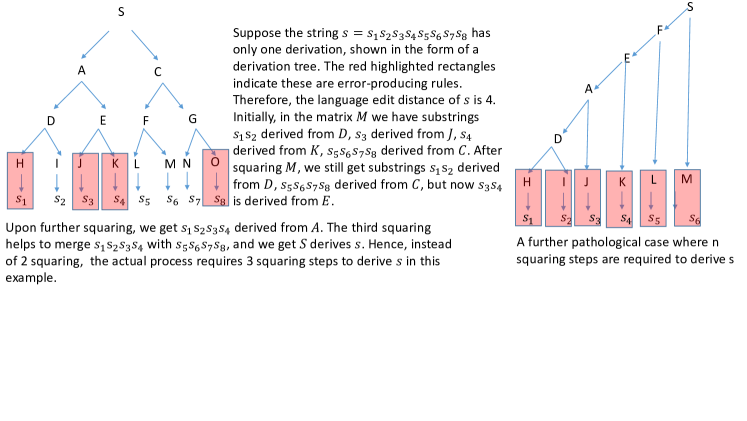
Figure 1: Example

This also illustrates replacing exact distance product computation by known “approximation” algorithm for distance product will not be sufficient. If we use a $(1+\epsilon)$-approximation for distance product each time when we multiply matrices in Valiant’s method, then the overall approximation can be as bad as $(1+\epsilon)^{n}$. With the best known bound for $\epsilon$ with $\tilde{O}(n^{\omega})$ running time [50], the approximation factor becomes $O(\frac{n}{polylog{n}})$. Lack of flexibility in recursively combining substrings is a major bottleneck. This arises because the underlying structure over which matrix product is defined is nonassociative.

We are able to overcome this significant difficulty by introducing several new ideas. Randomization plays a critical role. We restrict the number of possible edit distances to few distinct values, and use randomization carefully to maintain the language edit distance for each substring on expectation and show even for a long parse tree the variance does not blow up. A 1941 theorem by Erd$\ddot{o}$s and Tur$\acute{a}$n [15], and a construction by Ruzsa [36] allow to map the distinct edit distances maintained by our algorithm to a narrow range of possible scores such that each matrix product can be computed cheaply. This also leads to the first sub-cubic algorithm for stochastic context free grammar parsing near-optimally (Section 3).

2.1 Error Producing Productions & Assigning Scores

The first step of our algorithm is to introduce new error-producing rules in ${\mathcal{P}}(G)$, each of which adds one type of errors: insertion, deletion and substitution. Error-producing rules are assigned boolean scores, and our goal is to use the fewest possible error-producing rules to parse a given string $s$. If parsing $s$ must use error-producing rules with a total score of $k$, then $\mathrm{d}(G,s)=k$. The rules introduced are extremely simple and intuitive.

Substitution Rule. If there exists rule $A\rightarrow x_{1}|x_{2}|...|x_{l},~{}x_{i}\in\Sigma,i=1,2,...l$ for some $l\geq 1$, then cnsider adding an error-producing rule $A\rightarrow y_{1}|y_{2}|...|y_{l^{\prime}}$, such that $\{y_{1},y_{2},...,y_{l^{\prime}}\}=\Sigma\setminus\{x_{1},x_{2},...,x_{l}\}$. This rule corresponds to a single substitution error where a $x_{i}$ is substituted by a $y_{j}$. Each of these new rules referred as elementary substitution rule gets a score of $1$. However, instead of maintaining these rules explicitly, we maintain a single rule $A\rightarrow\$x_{1}x_{2}...x_{l}$, where $\$$ is a special symbol not occurring in $\Sigma$. This implicit representation, though violates CNF representation, has the same effect as maintaining $A\rightarrow y_{1}|y_{2}|...|y_{l^{\prime}}$ explicitly only the size of the rule is $l+2$ (counts the number of terminals and nonterminals on LHS and RHS). If we want to use $A\rightarrow y_{i}$ as an elementary substitution rule, we check if there exists a rule $A\rightarrow\$\alpha$ where $\alpha\in\Sigma^{*}$ and $y_{i}$ is not in $\alpha$. If so, we use $A\rightarrow y_{i}$ with score $1$ for parsing. This is the only type of rule which has more than two symbols on the RHS. But since they will be used at most once for every symbol in the input string, using them adds only $O(|G_{e}|^{2}n)$ to the running time, and is dominated by the running time of other operations.

Insertion Rule. For each $x\in\Sigma$, we add an error-producing rule $I\rightarrow x$ which corresponds to a single insertion error. Again the score for each of these rules referred as elementary insertion rule is $1$. We also introduce for each nonterminal $A\in{\mathcal{N}}$, a new rule $A\rightarrow IA$ to allow a single insertion right before a substring derivable from $A$. Further, we add a new rule $A\rightarrow AI$ for each nonterminal $A\in{\mathcal{N}}$ to let single insertion happen at the end of a substring derivable from $A$. Finally, we add a rule $I\rightarrow II$ to combine two insertion errors. These later rules that combine elementary insertion rule with other nonterminals have score $0$.

Deletion Rule For each $A\rightarrow x,~{}x\in\Sigma$, we add a rule $A\rightarrow\varepsilon$ with a score of $1$. We call them elementary deletion rules. Inclusion of these rules violate the CNF property, as in a CNF grammar, we are not allowed to have $\varepsilon$ on the RHS of any production except for $S\rightarrow\varepsilon$.

Observation 1.

$|G_{e}|=O(|G|)$.

Scoring. Each of the elementary error-producing rules gets a score of $1$ as described above. The existing rules and remaining new rules get a score of $0$. If a parsing of a string $s$ requires applying productions $\pi=P_{1},P_{2},...,P_{n}$ respectively then the parse has a score

$$score(\pi)=\sum_{i=1}^{n}score(P_{i}).$$

Let $G_{e}$ denote the new grammar after adding the error-producing rules. We prove in Lemma 1 and Lemma 2 that a string $s$ has a parse of minimum score $l$ if and only if $\mathrm{d}_{G}(G,s)=l$. Lemma 1 serves as a base case for Lemma 2.

Lemma 1.

For each string $s$, $d_{G}(G,s)=1$ if and only if there is a derivation sequence in $G_{e}$ to parse $s$ with a score of $1$, and none with score of $0$. And $d_{G}(G,s)=0$ if and only if there exists a derivation sequence in $G_{e}$ to parse $s$ with score of $0$.

Proof.

$d_{G}(G,s)=0$. Recall that all original productions of $G$ have score $0$ in $G_{e}$. For a string $s$ with $d_{G}(G,s)=0$, parsing in $G_{e}$ can only use these original productions of $G$ with a total score of $0$. To prove the other direction, if we use any of the error-producing productions, then to produce a terminal, one must use one of the elementary error-producing rules with score $1$. Hence, if $G_{e}$ parses a string $s$ with score $0$, it must use only original productions of $G$. Hence $d_{G}(G,s)=0$.

Claim 1.

$d_{G}(G,s)=1$ if and only if the minimum score of any parsing of $s$ in $G_{e}$ is $1$.

Let us first prove the “only if” part. So, $d_{G}(G,s)=1$. This single error has caused by either substitution or insertion or deletion.

First consider a single substitution error at the $l$th position. Let $s_{l}=b$. Suppose, if $s_{l}=a$ then $s\in{\mathcal{L}}(G)$. Considering $s_{l}=a$, obtain the left-most derivation of $s$ in $G$. Stop at the step in the left-most derivation when a production of the form $A\rightarrow a$ is applied to derive $s_{l}=a$. By definition of left-most derivation, we have a parsing step $\alpha A\beta\rightarrow\alpha a\beta$, where $\alpha\in\Sigma^{*}$, $\beta\in(\Sigma\cup\cal{N})^{*}$. Use $A\rightarrow b$ with a score of $1$ instead and keep all the remaining parsing steps identical to obtain a parse in $G_{e}$ with score $1$.

Now consider a single insertion error at the $l$th position, $l<n$, i.e., the string $s^{\prime}=s_{1}s_{2}..s_{l-1}s_{l+1}...s_{n}$ is in $\cal{L}(G)$. Consider the left-most derivation of $s^{\prime}$ in $G$. Stop at the step when a production of the form $A\rightarrow s_{l+1}$ is used to produce the terminal $s_{l+1}$. To parse $s$ in $G_{e}$, follow the parsing steps of $s^{\prime}$ in $G$ till $A\rightarrow s_{l+1}$ is applied. Instead use $A\rightarrow IA$ with score $0$, followed by $I\rightarrow s_{l}$ with score $1$ and $A\rightarrow s_{l+1}$ with score $0$. Now, continue the rest of the derivation steps of $s^{\prime}$ in $G$. Clearly, the score to parse $s$ in $G_{e}$ is $1$. If $l=n$, then use $S\rightarrow SI$ as the first production, derive $s_{1}s_{2}...s_{n-1}$ from $S$ as in $G$ and then use $I\rightarrow s_{n}$ with a score of $1$ to complete the parsing of $s$ in $G_{e}$.

Finally, consider a single deletion error. Suppose, the deletion happens right before the $l$th position, $l=1,..,n+1$. Then for some $y\in\Sigma$, the string $s^{\prime}=s_{1}s_{2}..s_{l-1}ys_{l}..s_{n}$ is in $\cal{L}(G)$. Consider a parse of $s^{\prime}$ in $G$. Consider the step in which a production of the form $B\rightarrow AC$ (or $B\rightarrow CA$) is used with subsequent application of $A\rightarrow y$ to produce the terminal $y$. Apply all the parsing steps of $s^{\prime}$, except $A\rightarrow y$, apply $A\rightarrow\varepsilon$ with score of $1$.

This completes the “only if” part.

We now prove the “if” part. We have a parse $\pi(s)=P_{1}P_{2}.....P_{r}$ of $s$ of score $1$ in $G_{e}$. Therefore, there exists exactly one $P_{i}$, $1\leq i\leq r$ which is an elementary error-producing rule. If $P_{i}$ is an elementary substitution rule $A\rightarrow y$ which is generated from the original rule $A\rightarrow x$, then replace in $s$ the symbol $y$ which $P_{i}$ produces by $x$ to map $s$ to ${\mathcal{L}}(G)$. Hence, $\mathrm{d}_{G}(G,s)=1$. Similarly, if $P_{i}$ is an elementary insertion rule $I\rightarrow y$, then delete $y$ from $s$ and remove $P_{i}$ as well all productions (there can be at most one such production) of the form $A\rightarrow AI$ or $A\rightarrow IA$. The remaining productions in $\pi(s)$ uses only original rules and parse $s$ after removal of symbol $y$ in $G$. Hence $\mathrm{d}_{G}(G,s)=1$. If $P_{i}$ is of the form $A\rightarrow\varepsilon$, then similarly modify $P_{i}$ to $A\rightarrow x\in{\mathcal{P}}(G)$ to obtain a modified string $s^{\prime}\in{\mathcal{L}}(G)$ with $dist(s,s^{\prime})=1$. Thus, $\mathrm{d}_{G}(G,s)=1$. ∎

This completes the proof. ∎

The following corollary follows directly from the above lemma.

Corollary 2.

Given any string $s\in\Sigma^{*}$, there exists a nonterminal $A\in{\mathcal{N}}(G)$ such that $A\xRightarrow{\ast}s$ with a parse score of $1$ in $G_{e}$ if and only if there exists a $s^{\prime}\in{\mathcal{L}}(G)$ such that $A\xRightarrow{\ast}s^{\prime}$ with score of $0$ in $G$, and $dist(s,s^{\prime})=1$.

Lemma 2.

Given any string $s\in\Sigma^{*}$, there exists a nonterminal $A\in{\mathcal{N}}(G)$ such that $A\xRightarrow{\ast}s$ with a parse of score $l$ in $G_{e}$ if and only if there exists a string $s^{\prime}\in\Sigma^{*}$ such that $A\xRightarrow{\ast}s^{\prime}$ in $G$ (and $G_{e}$ with a parse of score $0$) and $\mathrm{d}(s,s^{\prime})=l$. Thus if $l$ is the minimum score for deriving $A\xRightarrow{\ast}s$ in $G_{e}$ and if $A=S$, then $\mathrm{d}(G,s)=l$.

Proof.

Corollary 3 serves as a base case when $l=0$ and $l=1$. Suppose the result is true up to $l-1$.

Let us first assume that there exists nonterminal $A\in{\mathcal{N}}(G)$ such that $A\xRightarrow{\ast}s^{\prime}$ in $G$ with a parse of score $0$ and $\mathrm{d}(s,s^{\prime})=l$. Then to match $s$ with $s^{\prime}$, it requires exactly $l$ substitution, insertion and deletions in $s$. Consider the left-most edit position, correct it to obtain a string $s^{\prime\prime}$ such that $\mathrm{d}(s^{\prime\prime},s^{\prime})=l-1$. By induction hypothesis, there exists a parsing $\pi(s^{\prime\prime})$ of $s^{\prime\prime}$ of score $l-1$ starting from $A$. Now consider $s$, $s^{\prime\prime}$ and $\pi(s^{\prime\prime})$ and depending on the type of error, follow exactly the same argument as in Lemma 1 to obtain a parse of $s$ in $G_{e}$ with a score just one more than $\pi(s^{\prime\prime})$, that is, $l$ starting from $A$.

We now prove the other direction. Let the parse for $s$ in $G_{e}$, $\pi(s)=P_{1}P_{2}...P_{r}$, $P_{1}=A$, has a score of $l$, then it uses exactly $l$ elementary error-producing rules. Let $P_{i}$ be the left-most elementary error-producing rule. Depending on the type of the rule, follow exactly the same argument as in Lemma 1 to modify $P_{i}$ to obtain a string $s^{\prime\prime}$ such that $\mathrm{d}(s,s^{\prime\prime})=1$, and $s^{\prime\prime}$ has a parsing in $G_{e}$ with score exactly $l-1$ starting from $A$. Therefore, by induction hypothesis, there exists $A\xRightarrow{\ast}s^{\prime}$ in $G$ with a parse score of $0$ such that $dist(s^{\prime},s^{\prime\prime})=l-1$. Hence, $\mathrm{d}(s^{\prime},s)\leq l$.

This establishes the lemma. ∎

2.2 Parsing with At most $R$ Errors

The next step of our algorithm is to compute a $(n+1)\times(n+1)$ upper triangular matrix $M$ such that its $(i,j)$th entry contains all nonterminals that can derive the substring $s_{i}^{j-1}=s_{i}s_{i+1}...s_{j-1}$ using at most $R\geq 1$ elementary error-producing rules. We often use ${\mathcal{N}},{\mathcal{P}}$ when in fact we mean ${\mathcal{N}}(G_{e})$, ${\mathcal{P}}(G_{e})$ respectively. We start with a few definitions.

2.2.1 Definitions

Definition 4 (Operation-$r$).

We define a binary vector operation between $(A,u)$ and $(B,v)$ where $A,B\in{\mathcal{N}}$ and $u,v\in[0,1,2,...,n]$ as follows

$$(A,u)*_{r}(B,v) =(C,x)\text{ If }C\rightarrow AB\in\cal{P}\text{ and $x=u+v<r$}$$ (1)

$$=\phi\text{ otherwise}$$

Note the peculiarity of the above operation. $(A,u)*_{r}((B,v)*_{r}(D,y))$ may well be different from $((A,u)*_{r}(B,v))*_{r}(D,y)$. Therefore, the new binary operation is not associative. This is important to note, since non-associativity of the above operation is the main source of difficulty for designing efficient algorithms.

We omit $r$ to keep the representation of the operator concise whenever its value is clear from the context.

Definition 5 (Elem-Mult).

Given $T_{1}=\{(A_{1},u_{1}),(A_{2},u_{2}),...,(A_{k},u_{k})\}$ and $T_{2}=\{(B_{1},v_{1}),(B_{2},v_{2}),...,(B_{l},v_{l})\}$ for some $k,l\in\mathbb{N}\cup\{0\}$, define

$$T=T_{1}.T_{2}=\bigcup^{\min}_{\forall i=1,2,..,k,\text{ and}j=1,2,...,l}(A_{i},u_{i})*(B_{j},v_{j}).$$

where $\bigcup^{\min}$ implies if we have $(C,x_{1}),(C,x_{2}),....,(C,x_{i})$ involving the same nonterminal, we only keep $(C,\min\{x_{1},x_{2},..,x_{i}\})$.

We can define some operation on matrices in terms of the above where matrix elements are collection of tuples $(A\in\mathcal{N},u\in\{0,1,2,...,r\})$. We define matrix multiplication $a.b=c$ where $a$ and $b$ have suitable sizes as follows

$$c(i,k)=\bigcup_{j=1}^{n}a(i,j).b(j,k)$$ (Matrix-Mult)

The transitive closure of a square matrix is defined as

$$a^{+}=a_{1}\cup a_{2}\cup...$$

where $a_{1}=a$ and $a_{i}=\bigcup_{j=1}^{i-1}a_{j}.a_{i-j}$.

It is typical to compute transitive closure $a^{+}$ from $a$ by repeated squaring of $a$, so to compute $a^{n}$ requires $\lceil\log{n}\rceil$ squaring. This property does not hold here, again because the “.” operation is non-associative.

We will soon need to obtain a transitive closure of a matrix, where after each multiplication (possibly of two square submatrices (say) of dimension $m\times m$, $m\leq n$, we would need to perform some auxiliary tasks taking $O(m^{2}|G|^{2})$ time. Since the underlying matrix multiplication anyway needs $\Omega(m^{2}|G|^{2})$ time, the overall time for computing transitive closure will not change.

2.2.2 Algorithm

We are now ready to describe our algorithm.

Generating Deletion-$r$ sets :$D_{r}$

We let $r=n$ and first generate several sets $D_{1},D_{2},D_{3},D_{4},...,D_{n}$ where

$$D_{1}=\begin{array}[]{ll}\{(A,1)\,\mid\,A\rightarrow\varepsilon\in{\mathcal{P}}(G_{e})\}\cup(S,0)&\text{ if }S\rightarrow\varepsilon\in{\mathcal{P}}(G)\\ \{(A,1)\,\mid\,A\rightarrow\varepsilon\in{\mathcal{P}}(G_{e})\}&\text{ otherwise}\end{array}$$

We define $D_{2}=D_{1}\cup D_{1}.D_{1}$, and $D_{i}=D_{{i-1}}\cup D_{{i-1}}.D_{{i-1}}$. The following lemma establishes the desired properties of these sets.

Lemma 3.

For all $A\in{\mathcal{N}}(G_{e})$ if $A\xRightarrow{\ast}\varepsilon$ with a parse of score $u$ then $(A,u^{\prime})\in D_{u}$ where $u^{\prime}\leq u$ and if $(A,i)\in D_{u}$ then $A\xRightarrow{\ast}\varepsilon$ with a parse of score $i$ ($i$ may be larger than $u$). All the sets $D_{1},D_{2},...,D_{n}$ can be computed in $O(n|{\mathcal{P}}(G_{e})|)$ time.

Proof.

The claim is true for $D_{1}$ by construction. Suppose the claim is true till $i-1$ by induction hypothesis.

Now suppose $(A,u)\in D_{i}$ then either $(A,u)\in D_{i-1}$ or there exists $(B,v)\in D_{i-1},(C,x)\in D_{i-1}$ such that $A\rightarrow BC\in{\mathcal{P}}(G)$, and $u=v+x$ which serves as an evidence why $(A,u)\in D_{i}$. By induction hypothesis $A\xRightarrow{\ast}\varepsilon$ with a score of $u$ in the first case; in the second case induction hypothesis applies to $B$ and $C$, and by definition of “.” operator, we have the desired claim for $A$.

On the other hand, if $A\xRightarrow{\ast}\epsilon$ with a score of $u\leq n$, then either $A\rightarrow\varepsilon$–in that case $A\in D_{1}\subseteq D_{s}$, or $A\rightarrow BC\in{\mathcal{P}}(G)$ and each $B$ and $C$ derives $\varepsilon$ with a score of $u_{1}$ and $v_{1}$ respectively where $u_{1}\leq u-1,v_{1}\leq u-1$. Therefore, both $B$ and $C$ are in $D_{u-1}$ and hence $(A,u)$ is considered for inclusion in $D_{u}$. If $(A,u)$ is not in $D_{u}$ that only means there is some $u^{\prime}<u$ and $(A,u^{\prime})\in D_{u}$.

$D_{i}$ can be calculated from $D_{i-1}$ in $O(h)$ time where $h=|{\mathcal{P}}(G_{e})|$. We go through the list of productions $A\rightarrow BC$ in $G_{e}$ and check if both $B$ and $C$ are in $D_{i-1}$ to generate $A$. For each nonterminal $A$ thus generated we maintain its minimum score in $O(1)$ time. Taking union with $D_{i-1}$ also taken only $O(h)$ time. In fact $h$ only includes the productions of $G$ and the elementary deletion rules of $G_{e}$. Hence, all the $D_{1},D_{2},....,D_{n}$ can be computed in time $O(nh)$. ∎

Computing $TransitiveClosure^{+}$

We compute a $(n+1)\times(n+1)$ upper triangular matrix $M$ such that its $(i,j)$th entry contains all nonterminals that can derive the substring $s_{i}^{j-1}=s_{i}s_{i+1}...s_{j-1}$ using at most $R$ edit operations.

Let the input string be $s=s_{1}s_{2}...s_{n}\in\Sigma^{*}$.

1. First compute the $(n+1)\times(n+1)$ upper triangular matrix defined by

   $$b(i,i+1)=\{(A_{k},score(A_{k}\rightarrow x_{i}))\mid A_{k}\rightarrow x_{i}\}$$

   $$b(i,j)=\phi~{}~{}\text{for }j\neq i+1$$

2. Next, compute $b^{R}$, where for every entry $b^{R}(i,j)$ we follow the following subroutine.

   • $b^{R}(i,j)=b(i,j)$

   • For $count=1$ to $|G_{e}|$

     • $b^{R}(i,j)=b^{R}(i,j)\cup D_{n}.b^{R}(i,j)\cup b^{R}(i,j).D_{n}$

     • If there are multiple tuples involving same nonterminal $(A,u_{1}),(A,u_{2}),...,(A,u_{l}),l\geq 1$ only keep $(A,\min{\{u_{1},u_{2},..,u_{l}\}})$

   • End For

   • Discard any $(A,u)$ that appears with $u>R$.

   We could have used $D_{R}$ instead of $D_{n}$ here. But, since this subroutine will be repeatedly used in the final algorithm with $D_{n}$, we use $D_{n}$ here to avoid later confusion.

3. Finally, compute the transitive closure of $b^{R}$ but after each multiplication (possibly of two submatrices of dimension $m\times m$, $m<n$), multiply every entry $M(i,j)$ of the resultant $m\times m$ matrix by $D_{n}$ $|G_{e}|$ times.

   • For $count=1$ to $|G_{e}|$

     • $M(i,j)=M(i,j)\cup D_{n}.M(i,j)\cup M(i,j).D_{n}$

     • If there are multiple tuples involving same nonterminal $(A,u_{1}),(A,u_{2}),...,(A,u_{l}),l\geq 1$ only keep $(A,\min{\{u_{1},u_{2},..,u_{l}\}})$

   • End For

   • Discard any $(A,u)$ that appears with $u>R$.

   Each iteration of the for loop takes time $O(|G_{e}|)$. Hence overall time for updating each matrix entry is $O(|G_{e}|^{2})$. Therefore, total time taken for this auxiliary operation is $O(m^{2}|G_{e}|^{2})$. Since, each entry of $M$ may contain $|G_{e}|$ nonterminals, assuming each product takes $\Omega(m^{2}|G_{e}|^{2})$ (which indeed will be the case) time, adding this auxiliary operation does not change the time to compute the overall transitive closure. To distinguish it from normal transitive closure, we call it $TransitiveClosure^{+}$. Therefore, this step computes $M=TransitiveClosure^{+}(b^{R})$.

The following lemma proves the correctness.

Lemma 4.

$(A_{k},u)\in M(i,j)$, if and only if $A_{k}\xRightarrow{\ast}s_{i}^{j-1}$ in $G_{e}$ with a parse score of $u\leq R$, and there does not exist any $u^{\prime}<u$ such that $A_{k}\xRightarrow{\ast}s_{i}^{j-1}$ with parse score of $u^{\prime}$.

Proof.

The proof is by an induction on length of $s_{i}^{j-1}$.

Base case. Note that $b$ is upper triangular. This implies $M(i,i+1)=b^{R}(i,i+1)$. Now by construction of $b$, $M(i,i+1)$ contains all nonterminals that derive $x_{i}$ either with score $0$ or by a single insertion error, or by a single substitution error. The only case remains when $x_{i}$ may be derived by deletion of symbols either on the right, or on the left, or both.

Consider a derivation of $x_{i}$ which involves deletion error. Then the first production used to derive $x_{i}$ must be of the form $C_{0}\rightarrow B_{1}C_{1}$ for $C_{0},B_{1},C_{1}\in{\mathcal{N}}(G_{e})$ and among $B_{1}$ and $C_{1}$ one must derive $\varepsilon$. If $B_{1}\Rightarrow\varepsilon$ and $C_{1}\rightarrow x$ or $C_{1}\Rightarrow\varepsilon$ and $B_{1}\rightarrow x$, then on the first multiplication by $D_{n}$, $C_{0}$ will be included in $b^{R}$ if the total score of it is less than $R$. Otherwise, w.l.o.g say $B_{1}\Rightarrow\varepsilon$, and $C_{1}\rightarrow B_{2}C_{2}$. Note that $C_{1}\neq C_{0}$ because otherwise, it is sufficient to consider derivation from $C_{1}$. One of $B_{2}$ or $C_{2}$ must derive $\varepsilon$, if the other directly derives $x_{1}$, then both $C_{0}$ and $C_{1}$ will be included in $b^{R}$ after two successive multiplications by $D_{n}$. If none of $B_{2}$ or $C_{2}$ derives $\varepsilon$, then again w.l.o.g we can assume $B_{2}\Rightarrow\varepsilon$ and $C_{2}\rightarrow B_{3}C_{3}$ where again $C_{2}\neq C_{1}\neq C_{0}$–this process can continue at most $|G_{e}|$ steps. Thereby, after $|G_{e}|$ successive multiplications with $D_{n}$, $M(i,i+1)$ contains all the nonterminals that derive $s_{i}$ with a score of at most $R$.

Induction Hypothesis. Suppose, the claim is true for all substrings of length up to $l$.

Induction. Consider a substring of length $l+1$, say, $s_{i}^{i+l+1}$. If $M(i,i+l+2)$ contains $A_{k}$, then either

(1) there must be some $j$, $i<j<i+l+2$ (because $M$ is upper triangular) such that $M(i,j)$ contains a $(B_{k},u_{1})$ and $M(j,i+l+2)$ contains a $(C_{k},u_{2})$ such that $A_{k}\rightarrow B_{k}C_{k}$ and $u_{1}+u_{2}<R$, or

(2) $A_{k}$ is included in $M(i,i+l+2)$ due to multiplications by $D_{n}$.

For (1) by induction hypothesis $B_{k}$ derives $s_{i}^{j-1}$ with a parse of score $u_{1}$ and $C_{k}$ derives $s_{j}^{i+l+1}$ using a parse of score $u_{2}$. Since $A_{k}\rightarrow B_{k}C_{k}$ has a score of $0$, $A_{k}$ derives $s_{1}^{i+l+1}$ using a parse of score $u_{1}+u_{2}<R$. For (2) there must exist a $(B,u_{1})\in M(i,i+l+2)$, $B\xRightarrow{\ast}s_{i}^{i+l+1}$ with score of $u_{1}$ and a derivation sequence starting from $A_{k}$ where each production contains two nonterminals on RHS with one of them producing $\varepsilon$ and the derivation sequence terminates when $B$ is generated. In that case again, $A_{k}\xRightarrow{\ast}s_{i}^{i+l+1}$ and is included if and only if the total score of the derivation sequence including the score for $B$ is at most $R$.

For the other direction, note that for every index $j$, $i<j<i+l+2$, $M(i,j)$ and $M(j,i+l+2)$ contain all the nonterminals that derive $s_{1}^{j-1}$ and $s_{j}^{i+l+2}$ respectively within a parse score of at most $R$. Hence, by the definition of $TransitiveClosure^{+}$, if $(B_{k},s_{1})\in M_{i,j},B_{k}\xRightarrow{\ast}s_{i}^{j-1}$ with a parse score of $u_{1}$ and $(C_{k},s_{2})\in M(j,i+l+2),C_{k}\xRightarrow{\ast}s_{j}^{i+l+1}$ with a parse score of $u_{2}$ and we have $u=u_{1}+u_{2}<R$ and $A_{k}\rightarrow B_{k}C_{k}\in{\mathcal{P}}$, then $(A_{k},u)\in M(j,i+l+2)$. Therefore, $M(j,i+l+2)$ contains all the nonterminals that derive $s_{i}^{i+l+1}$ by decomposition (that is the first production applied to derive $s_{i}^{i+l+1}$ has two nonterminals on the RHS, none of which produces $\varepsilon$ ) with a score of at most $R$ (even before multiplication with $D_{n}$).

The only case remains when there is a derivation tree starting from $A$ to derive $s_{i}^{i+l+1}$ by application of a rule of the form $A\rightarrow BC$, where either $B$ or $C$ produces $\varepsilon$. We grow the derivation tree for each nonterminal that does not produce $\varepsilon$, and stop as soon as the current production (say) $X\rightarrow YZ$ considered generates two nonterminals $Y,Z$ none of which produces $\varepsilon$. We know $(X,u^{\prime})$ must be in $M(i,i+l+2)$ if $u^{\prime}\leq R$. Then we argue as in the base case for incorporating deletion errors that $(A,u)$ must be included in $M(j,i+l+2)$, if $u\leq R$. Note that $u>u^{\prime}$, hence if $(X,u^{\prime})\notin M(j,i+l+2)$, $(A,u)$ cannot be in $M(j,i+l+2)$. ∎

Corollary 3.

For all $A_{k}\in{\mathcal{P}}(G_{e})$, $A_{k}\in M(i,j)$, if and only if $A_{k}\xRightarrow{\ast}s_{i}^{j-1}$ in $G_{e}$ with score of at most $R$ such that $\exists t^{\prime}\in{\mathcal{L}}(G)$ with $\mathrm{d}(s_{i}^{j-1},t^{\prime})\leq R$ and $A_{k}\xRightarrow{\ast}t^{\prime}$ with a score of $0$.

Proof.

The proof follows from Lemma 4 and Lemma 2. ∎

2.2.3 Running Time Analysis

Therefore, the complete information of all substrings of $s$ that can be derived from a nonterminal in $G_{e}$ within a parse of score of at most $R$ is available in $M$. We now calculate the time needed to compute $M$. The analysis goes in two steps.

$\bullet$ Step 1. Show that time needed to compute $M$ ($TransitiveClosure^{+}(b^{R})$) is asymptotically same as the time needed to compute a single $Matrix\text{-}Mult$.

$\bullet$ Step 2. Show that time needed to compute a single $Matrix\text{-}Mult$ is $O(\min{\{R|G|^{2}n^{\omega},|G|^{2}T(n)\}})$, where $T(n)$ is the time required to compute distance product of two $n$ dimensional square matrices.

Step 1. Reduction from $TransitiveClosure^{+}$ to $Matrix\text{-}Mult$

This reduction falls off directly from the proof of Valiant [41]. We briefly explain it here and detail the necessary modifications.

First of all note that computing $TransitiveClosure^{+}$ has same asymptotic time as computing $TransitiveClosure$. Therefore, we can just focus on the time complexity of $TransitiveClosure$ computation of $b^{R}$.

We start with $b^{R}$. Recall our definition of $Elem\text{-}Mult$. Suppose, we do not consider the second component, that is score when performing $Elem\text{-}Mult$. So given $(A,s)$ and $(B,t)$, if $\exists C\rightarrow AB$, when multiplying $(A,s)$ and $(B,t)$, we generate $C$ irrespective of score $s+t$. Let us refer it as $Elem^{\prime}\text{-}Mult$. This is exactly the situation handled by Valiant. In Valiant’s own words, “several analogous procedures for the special case of Boolean matrix multiplication are known …. However, these all assume associativity, and are therefore not applicable here. Instead of the customary method of recursively splitting into disjoint parts, we now require a more complex procedure based on “splitting with overlaps”. Fortunately, and perhaps surprisingly, the extra cost involved in such a strategy can be made almost negligible.”

Valiant’s Proof Sketch.

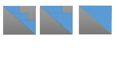
Figure 2: Decomposition into overlapping parts. While Valiant’s Method computes transitive closure in asymptotically same time as single matrix multiplication, there could be cells in the matrix that takes part in $O(n)$ multiplication steps.

Let $c$ be an upper triangular matrix. Define $c^{+(r:s)}$ to be the result of the following operations (i) collapse $c$ by removing all elements $c(i,j)$ where $r<i\leq s$ and $r<j\leq s$, (ii) compute the transitive closure of the $(n+r-s)\times(n+r-s)$ matrix, and (iii) expand the matrix back to its original size by restoring the elements that were removed to their original position.

Valiant’s result is based on the following observation. If the submatrices of $c$ specified by by $[1\leq i,j\leq s]$, and $[r<i,j\leq n]$ are both already transitively closed, and $s\geq r$ then

$$c^{+}=(c\cup(c.c))^{+(r:s)}$$ (Valiant-Eq)

This expresses the facts that to obtain $c^{+}$ we just need to multiply $c$ once and then consider the submatrix $[1\leq i\leq r,s<j\leq n]$. This gives a divide-and-conquer approach and leads to the following theorem. Recall again, we are working with a modified version $Elem^{\prime}\text{-}Mult$ of $Elem\text{-}Mult$.

Theorem (Theorem $2$ [41].).

Let $m(n)$ denote the time required to compute a single matrix multiplication of $n$-dimensional square matrices and $t(n)$ the time required to compute the transitive closure. If $m(n)\geq n^{\gamma},\gamma\geq 2$, then

$$t(n)=m(n)+O(n^{2})~{}~{}~{}\text{if }\gamma>2$$

$$t(n)=m(n)\log{n}+O(n^{2})~{}~{}~{}\text{if }\gamma=2.$$

To incorporate $Elem\text{-}Mult$ is trivial. The above theorem and the relation $Valiant\text{-}Eq$ do not change at all, only $m(n)$ is replaced by $m^{\prime}(n)$ which now represents the time needed for our $Matrix\text{-}Mult$ operation, and not the one used by Valiant. Since $TransitiveClosure^{+}$ has same asymptotic time as $TransitiveClosure$, we get the following lemma.

Lemma 5.

Let $m^{\prime}(n)$ and $t^{\prime}(n)$ denote the time required to compute a single matrix multiplication of $n$ dimensional square matrices according to $Matr\text{-}Mult$ and $TransitiveClosure^{+}$ respectively. If $m^{\prime}(n)\geq n^{\gamma},\gamma\geq 2$ then

$$t^{\prime}(n)=m^{\prime}(n)+O(n^{2})~{}~{}~{}\text{if }\gamma>2$$

$$t^{\prime}(n)=m^{\prime}(n)\log{n}+O(n^{2})~{}~{}~{}\text{if }\gamma=2.$$

Reduction from $Matrix\text{-}Mult$ to Distance Production Computation.

This reduction is simple.

Given two matrices $a$ and $b$ each of dimension $n\times n$, we wish to compute $c$ such that

$$c(i,j)=\bigcup_{k=1}^{n}a(i,k).b(k,j)$$

To do so, we compute two real matrices $a^{\prime}$ of dimension $(hn,n)$ and $b^{\prime}$ of dimension $(n,hn)$, from $a$ and $b$ respectively where $|h|=|{\mathcal{N}}(G_{e})|$ Initially all the cells of $a^{\prime}$ and $b^{\prime}$ are zeros.

To construct $a^{\prime}$ from $a$, we reserve $h$ consecutive rows for each row index $p$ of $a$. For each $(A_{i},x)\in a(p,q)$, $\forall p,q\in\{1,2,..,n+1\}$ we set $a^{\prime}((p-1)h+i,q)=x$.

To construct $b^{\prime}$ from $b$, we reserve $(R+1)h$ consecutive columns for each column index $q$ of $b$. For each $(A_{j},y)\in b(p,q)$, $\forall p,q\in\{1,2,..,n+1\}$ we set $b^{\prime}(p,(q-1)h+j)=y$.

We compute the distance product $c^{\prime}$ of $a^{\prime}$ and $b^{\prime}$ in time $O(h^{2}T(n))$.

To construct $c$ from $c^{\prime}$, consider all the rows $(p-1)h+1\leq i\leq ph$, and all the columns $(q-1)h+1\leq j\leq qh$, if $c^{\prime}(i,j)=z$ then if $i-(p-1)h=x$, $j-(q-1)h=y$, $B\rightarrow A_{x}A_{y}\in{\mathcal{P}}(G_{e})$, generate $(B,z)$ as a candidate to include in $c(p,q)$. After generating all the candidates for each nonterminal $B$ if $(B,u_{1}),(B,u_{2}),...,(B,u_{i}),u_{1}\leq u_{2}\leq...u_{i}$ are all candidates–include only $(B,u_{1})$ in $c(p,q)$.

We maintain a list of all productions. To obtain $c(i,j)$, we go through this list and for each production $B\rightarrow A_{x}A_{y}$ we check appropriate cells for $A_{x}$ and $A_{y}$ to obtain the score for $B$. Therefore, $c(i,j)$ can be constructed in time $O(h)$. Therefore, total time to compute $c^{\prime}$ is $O(h^{2}T(n))$ and time to compute $c$ from $c^{\prime}$ is $O(hn^{2})$. That the reduction is correct follows directly from the correctness proof of reducing distance product to ordinary matrix product computation [5, 40], and the way the matrices are computed. The details are simple and left to the reader.

Overall this takes $O(|G_{e}|^{2}T(n))$ time.

If we set $R=n$ and each $Matrix\text{-}Mult$ takes time $O(|G_{e}|^{2}T(n))$ and $TransitiveClosure^{+}$ can also be computed in $O(|G_{e}|^{2}T(n))$ time (assuming $T(n)=o(n^{2})$, if $T(n)=O(n^{2})$, an additional $\log{n}$ term will be added in the running time. Therefore, we get the following proposition.

Proposition 1.

Given a grammar $G=({\mathcal{N}},\Sigma,{\mathcal{P}},S)$, and a string $s\in\Sigma^{*}$, language edit distance $\mathrm{d}_{G}(G,s)$ can be computed exactly in $O(|G|^{2}T(n))$ time.

Proof.

Set $R=n$, and if $(S,x)\in M(1,n+1)$ return $x$. Note that $(S,n)$ is a candidate for inclusion in $M(1,n+1)$ where $S$ generates $s$ by all substitutions. Hence, there is an entry with nonterminal $S$ in $M(1,n+1)$. By Lemma 4 $\mathrm{d}_{G}(G,s)=x$. The total time taken is $O(|G_{e}|^{2}T(n))$. Since $|G_{e}|=O(|G|)$, we get the desired bound in the running time. ∎

With little bookkeeping, the entire parsing information for $s$ can also be stored. We elaborate on that in the appendix.

Reduction from $Matrix\text{-}Mult$ to Ordinary Matrix Multiplication.

$Matrix\text{-}Mult$ can be done much faster in $O(|G|^{2}|R|n^{\omega})$ time when we obtain parsing information for all substrings with score of at most $R$.

We use the reduction of distance product computation to ordinary matrix multiplication by Alon, Galil and Margalit [5] and Takaoka [40]. Given $a$ and $b$, we first create the matrices $a^{\prime}$ and $b^{\prime}$ as above of dimension $nh\times n$ and $n\times nh$ respectively. Then if $a^{\prime}(i,k)=x$, we set $a^{\prime}(i,k)=(nh+1)^{M-x}$ and if $b(k,j)=y$, we set $b^{\prime}(k,j)=(nh+1)^{M-y}$. We now calculate ordinary matrix product of $a^{\prime}$ and $b^{\prime}$ to obtain $c^{\prime}$ in time $O(h^{2}n^{\omega})$. In fact the time taken is $O(R\omega(nh,n,nh))$ which represents the time to multiply two rectangular matrices of dimensions $nh\times n$ and $n\times nh$ respectively.

If $c^{\prime}(i,j)=z$, then we set $c^{\prime}(i,j)=2R-\lceil\log_{(nh+1)}{z}\rceil$. After that, we retrieve $c$ from $c^{\prime}$ as before. Using this construction, we not only can compute $\min_{k}(a^{\prime}(i,k)+b^{\prime}(k,j))$, but we can also compute all distinct (at most $R^{2}$) sums $a^{\prime}(i,k)+b^{\prime}(k,j)$, k=1,2,..,n.

We maintain a list of all productions. To obtain $c(i,j)$, we go through this list and for each production $B\rightarrow A_{x}A_{y}$ we check appropriate cells for $A_{x}$ and $A_{y}$ to obtain the score for $B$. This takes at most $O(R)$ time. Hence $c(i,j)$ can be constructed in time $O(Rh)$ time. Therefore, total time to compute $c^{\prime}$ is $O(R\omega(nh,n,nh))$ and time to compute $c$ from $c^{\prime}$ is $O(Rhn^{2})$. That the reduction is correct follows directly from the correctness proof of reducing distance product to ordinary matrix product computation [5, 40], and the way the matrices are computed. The details are simple and left to the reader.

Therefore a single $Matrix\text{-}Mult$ operation can be done in time $O(R\omega(nh,n,nh))$. Together with Lemma 5 this proves that parsing strings with score at most $R$ (and the complete parsing information of all its substrings) can be obtained in $O(R\omega(nh,n,nh)+h^{2}n^{2})$ time.

Lemma 6.

Given $G_{e}$ and string $s\in\Sigma^{*}$, one can compute a $(n+1)\times(n+1)$ matrix $M$ in $O(R\omega(n|G_{e}|,n,n|G_{e}|)+|G_{e}|^{2}n^{2})$ time such that its $(i,j)$th entry contains all nonterminals that can derive the substring $s_{i}^{j}$ with a parse of score at most $R$.

2.2.4 $Matrix\text{-}Mult$ with $R$ Distinct Scores

Before, we can describe the final algorithm, we need one more step. We saw when the values are bounded by $R$, $Matrix\text{-}Mult$ can be solved in $O(|G|^{2}Rn^{\omega}+|G|^{2}Rn^{2})$ time. We extend this to handle the case when there could be $R$ distinct values in the matrix, but with arbitrary values.

We first give a simple construction by reducing the distance product computation with $R$ distinct values to boolean matrix multiplication.

Reduction to boolean matrix multiplication

Given two matrices $a$ and $b$ each of dimension $n\times n$, we wish to compute $c$ such that

$$c(i,j)=\bigcup_{k=1,2,..,n}^{\min}a(i,k).b(k,j)$$

There can be at most $R+1$ distinct integer entries $v_{0}=0<v_{1}<v_{2}<..<v_{R}<n$ in $a$ and $b$.

To do so, we compute two boolean matrices $a^{\prime}$ of dimension $((R+1)hn,n)$ and $b^{\prime}$ of dimension $(n,(R+1)hn)$, from $a$ and $b$ respectively where $|h|=|{\mathcal{N}}(G_{e})|$. Initially all the cells of $a^{\prime}$ and $b^{\prime}$ are zeros.

To construct $a^{\prime}$ from $a$, we reserve $(R+1)h$ consecutive rows for each row index $p$ of $a$. For each $(A_{i},v_{x})\in a(p,q)$, $\forall p,q\in\{1,2,..,n+1\}$ we set $a^{\prime}((p-1)h(R+1)+(i-1)(R+1)+(x+1),q)=1$.

To construct $b^{\prime}$ from $b$, we reserve $(R+1)h$ consecutive columns for each column index $q$ of $b$. For each $(A_{j},v_{y})\in b(p,q)$, $\forall p,q\in\{1,2,..,n+1\}$ we set $b^{\prime}(p,(q-1)h(R+1)+(j-1)(R+1)+(y+1))=1$.

We compute the boolean product $c^{\prime}$ of $a^{\prime}$ and $b^{\prime}$ in time $O(R^{2}h^{2}n^{\omega})$.

To construct $c$ from $c^{\prime}$, consider all the rows $(p-1)h(R+1)+1\leq i\leq ph(R+1)$, and all the columns $(q-1)h(R+1)+1\leq j\leq qh(R+1)$, if $c^{\prime}(i,j)=1$ then if $i-(p-1)h(R+1)=(s-1)h+z$, $j-(q-1)h(R+1)=(t-1)h+x$, and $B\rightarrow A_{s}A_{t}\in{\mathcal{P}}(G_{e})$, generate $(B,v_{z}+v_{w})$ as a candidate to include in $c(p,q)$. After generating all the candidates for each nonterminal $B$ if $(B,u_{1}),(B,u_{2}),...,(B,u_{i}),u_{1}\leq u_{2}\leq...u_{i}$ are all candidates–include only $(B,u_{1})$ in $c(p,q)$.

We maintain a list of all productions. To obtain $c(p,q)$, we go through this list and for each production $B\rightarrow A_{s}A_{t}$ we check if $A_{s}$ and $A_{t}$ are present in the appropriate cells of $c^{\prime}$. This takes at most $O(R^{2})$ time. Hence $c(p,q)$ can be constructed in time $O(R^{2}h)$ time. Therefore, total time to compute $c^{\prime}$ is $O(R^{2}h^{2}n^{\omega})$ and time to compute $c$ from $c^{\prime}$ is $O(R^{2}hn^{2})$. Proving this construction is correct, is an easy exercise and left to the reader.

Thus, we can compute $a.b$ by first creating $a^{\prime}$, $b^{\prime}$, performing their boolean matrix multiplication $c^{\prime}$ and then obtaining $c$ from it using the above relation. The total time taken is $O(n^{2}R^{2}h+n^{\omega}R^{2}h^{2})$. ∎

We now discuss an alternate construction using which gives slightly worse dependency on $\frac{1}{\epsilon}$ in the final algorithm, but brings in a different perspective and may be useful in other contexts.

Sidon Sequences.

A Sidon sequence is a sequence $\mathcal{G}=(g_{1},g_{2},g_{3},...)$ of natural numbers in which all pairwise sums $g_{i}+g_{j}$, $i\leq j$ are different. The Hungarian mathematician Simon Sidon introduced the concept in his investigations of Fourier series in 1932. An early result by Erd$\ddot{o}$s and Tur$\acute{a}$n showed that the largest Sidon subset of $\{1,2,...,n\}$ has size $\sim\sqrt{n}$. There are several constructions known for Sidon sequences. A greedy algorithm gives a construction of size $k$ Sidon sequence from $O(k^{3})$ elements. Better constructions matching $O(k^{2})$ bound are known due to Ruzsa, Bose, Singer (for comprehensive literature survey see [31]).

Our Construction.

Given $R$ distinct values $v_{1}<v_{2}<v_{3}<...<v_{R}$ that may appear during $Matrix\text{-}Mult$, we create a size $R$ Sidon sequence ${\mathcal{G}}_{R}=(g_{1},g_{2},...,g_{R})$, $g_{1}<g_{2}<...<g_{R}$, and define map $f(v_{i})=g_{i}$. By the property of Sidon sequences, given a sum $g=g_{i}+g_{j}$, we can uniquely detect $g_{i}$ and $g_{j}$. We can keep a look-up table and do a binary search to find $g_{i}$ and $g_{j}$ given $g$ in $O(\log{R})$ time. By known construction $g_{R}=O(R^{2})$. The property of Sidon sequence ensures that all pair-wise sums are disjoint. Therefore, if we define $f(v_{i})=g_{i}$ by looking at the sum of $g_{i}+g_{j}$, we can identify $v_{i}$ and $v_{j}$. It is possible that $v_{i}+v_{j}<v_{k}+v_{l}$ but $g_{i}+g_{j}>g_{k}+g_{l}$, and vice versa.

Our reduction of $Matrix\text{-}Mult$ to ordinary matrix multiplication when values are bounded by $R^{2}$ uses an old construction by Alon, Galil, Margalit [5] and Takaoka [40] using which we can compute for each $(i,j)$ all distinct $a_{i,k}+b_{k,j}$, $k=1,2,..,n$ in $O(R^{4}n^{\omega}|G|^{2})$ time. The construction maps $a^{\prime}(i,j)=(nh+1)^{R^{2}-a_{i,j}}$ and $b^{\prime}(j,k)=(nh+1)^{R^{2}-b_{j,k}}$. Hence if $c^{\prime}=a^{\prime}*b^{\prime}$ where $*$ is ordinary matrix multiplication, then

$$c^{\prime}(i,j)=\sum_{k=1}^{n}(nh+1)^{2R^{2}-(a_{i,k}+b_{k,j})}$$

We can now find all distinct sums $2R^{2}-(a_{i,k}+b_{k,j})$ (and hence $a_{i,k}+b_{k,j}$), $k=1,2,..,n$ by repeatedly finding the largest exponent of $(nh+1)$ contributing to $c^{\prime}(i,j)$, that is by calculating $\lfloor\log_{(nh+1)}{c^{\prime}(i,j)}\rfloor$ and setting $c^{\prime}(i,j)=c^{\prime}(i,j)-\left\lfloor\frac{c^{\prime}(i,j)}{(nh+1)^{\lfloor\log_{(nh+1)}{c^{\prime}(i,j)}\rfloor}}\right\rfloor(nh+1)^{\lfloor\log_{(nh+1)}{c^{\prime}(i,j)}\rfloor}$ for the next iteration. Since there are at most $R^{2}$ distinct sums, and operating on these large numbers require $O(R^{2}\log{R})$ time, the overall time required is $\tilde{O}(R^{4}n^{\omega})$. Therefore, from the mapping $f$, we only require that the sum $f(v_{i})+f(v_{j})$ uniquely identifies $v_{i}$ and $v_{j}$. Then, from these at most $R^{2}$ distinct pairs, we can find the one with minimum sum in $O(R^{2})$ time per entry. Using this alternate approach gives a dependency of $\frac{1}{\epsilon^{8}}$ in the final algorithm instead of $\frac{1}{\epsilon^{4}}$ that is obtained using reduction to boolean matrix multiplication.

We note that Yuster’s construction to compute APSP in subcubic time when the number of distinct weight edges is not too many [47] may be applied here. But even for $R=O(1)$ their construction yields an $O(n^{2.5})$ algorithm (see Lemma 3.3 [47]), and hence provides much worse bound in our context.

2.3 Final Algorithm

Given an $\epsilon>0$, let $\delta=\frac{\epsilon^{2}}{16}$. we set $R=\log_{(1+\delta)}(n)$. We start with $b^{C}$ where $C$ is some constant say $10$, and compute $M^{C}=TransitiveClosure^{+}(b^{C},C)$.

We now define a new operation $TransitiveClosure^{++}$ which is same as $TransitiveClosure^{+}$ except we do some further auxiliary processing before and after each $Matrix\text{-}Mult$ (of possibly submatrices).

After every $Matrix\text{-}Mult$ (possibly of submatrices) and also after multiplying by $D_{n}$ each time, for every $(A,y)$ appearing in the current matrix, if $y=(1+\delta)^{r}+k$, where $k$ is any real number in $(0,\delta(1+\delta)^{r})$, $r=0,1,2,..,\lceil\log_{(1+\delta)}(n)\rceil$ then set

$$y=\left\{\begin{array}[]{cc}(1+\delta)^{r}&\text{ with probability }\frac{\delta(1+\delta)^{r}-k}{\delta(1+\delta)^{r}}\\ (1+\delta)^{r+1}&\text{ with probability }\frac{k}{\delta(1+\delta)^{r}}\end{array}\right.$$

Clearly, the number of distinct parsing scores that can appear on any tuple $(A,y)$ during the computation of $TransitiveClosure^{++}$ is bounded by $\lceil\log_{(1+\delta)}{n}\rceil$. Multiplying two submatrices of dimension $m\times m$ requires time $\Omega(|G_{e}|^{2}m^{2})$, whereas this auxiliary $Round$ operation can be performed in $O(m^{2})$ time. Hence overall the asymptotic time taken is not affected due to $Round$.

Before multiplying any two submatrices of (say) dimension $m\times m$, map $R=\lceil\log_{1+\delta}{n}\rceil$ possible parsing scores to $O(R^{2})$ Sidon sequences as discussed in Section 2.2.4. And, after the $Matrix\text{-}Mult$ is completed infer the actual sum from the inverse mapping from Sidon sequence to original (possibly previously rounded) values.

Hence, overall the time to compute $TransitiveClosure^{++}(M^{C},R)$ is same as $TransitiveClosure^{+}(M^{C},R^{2})$. The blow-up from $R$ to $R^{2}$ comes from mapping to Sidon sequences and inverse mapping to original sequences before and after each $Matrix\text{-}Mult$.

Starting from $M^{C}$ we repeat the process of computing $TransitiveClosure^{++}(M^{C},R)$ $\eta=6\log{n}$ times and obtain matrices ${\mathcal{M}}_{1},{\mathcal{M}}_{2},.....,{\mathcal{M}}_{\eta}$.

For each substring $s_{i}^{j-1}$ we consider the estimates given by $(S,d^{i:j}_{k})\in{\mathcal{M}}_{k}(i,j)$ $k=1,2,...,\eta$. Note that using the productions $S\rightarrow SI,I\rightarrow II$ and $I\rightarrow x,x\in\Sigma$, $S$ can always derive $s_{i}^{j-1}$ within edit distance $|j-i|$. Thus there always will be a tuple of the form $(S,d_{k}^{i:j})\in{\mathcal{M}}_{k}(i,j)$ for all $\eta=1,2,..,k$ and $1\leq i,j\leq(n+1)$. Let $d_{med}^{i:j}$ denote the median of these $\eta$ estimates. We return $d_{med}^{i:j}$ as the estimated edit score for $s_{i}^{j-1}$.

The parsing information for any substring $s_{i}^{j-1}$ can also be obtained in time $O(j-i)$ by small additional bookkeeping. We elaborate on it in the appendix.

2.3.1 Analysis

While the running time bound has already been established, we now analyze the performance of the above algorithm in terms of approximating language edit distance.

Consider any ${\mathcal{M}}_{k}$ and let us abuse notation and use ${\mathcal{M}}$ to denote it. Consider any substring $s^{\prime}=s_{i}^{j-1}$. Given a parse tree ${\mathcal{T}}$, we say ${\mathcal{M}}$ retains ${\mathcal{T}}$ if for every intermediate nonterminal $A$ of ${\mathcal{T}}$ deriving some substring $s_{i^{\prime}}^{j^{\prime}-1}$ the corresponding entry $(A,x)\in{\mathcal{M}}(i,j)$ contains the estimated value of parsing score of $A$ in ${\mathcal{T}}$. Therefore, $x$ is the actual estimate of parsing score of $A$ in ${\mathcal{T}}$ if ${\mathcal{T}}$ is retained.

Let $P$ be the parse tree corresponding to the estimate $\hat{e_{P}}$ returned by ${\mathcal{M}}[i,j]$ when $e_{P}$ is the actual parsing score for it. Let $O$ be the optimum parse tree for $s^{\prime}$ with minimum edit distance $e_{O}$. Since, each cell ${\mathcal{M}}(i^{\prime},j^{\prime})$ $1\leq i^{\prime},j^{\prime}\leq(n+1)$ contains all nonterminals that can derive substring $s_{i^{\prime}}^{j^{\prime}-1}$, the reason we do not return $O$ is simply because if we had retained $O$ throughout, its estimated score $\hat{e_{O}}\geq\hat{e_{P}}$ .

We now show that $\hat{e_{P}}\in[(1-\epsilon)e_{P},(1+\epsilon)e_{P}]$ and similarly $\hat{e_{O}}\in[(1-\epsilon)e_{O},(1+\epsilon)e_{O}]$ with high probability. Therefore,

$$e_{O}\leq e_{P}\leq(1+\epsilon)\hat{e_{P}}\leq(1+\epsilon)\hat{e_{O}}\leq(1+\epsilon)^{2}e_{O}\approx(1+2\epsilon)e_{O}$$ (ApproxEstimate)

We now prove $ApproxEstimate$.

Lemma 7.

${\sf E}\left[\hat{e_{P}}\right]=e_{P}$.

Proof.

Consider the parse tree $P$ and let $P^{\prime}$ denote the truncated parse tree after the algorithm completes execution of $TransitiveClosure^{+}(b^{C},C)$. The leaves of $P^{\prime}$ denote the exact parsing scores corresponding to the associated nonterminals by Lemma 4 and due to exact computation of $D_{n}$. Hence, if $l_{1},l_{2},...,l_{m}$ are the leaves of $P^{\prime}$ and $score(l_{i})$ is the score computed by $TransitiveClosure^{+}(b^{C},C)$ or $D_{n}$, then $e_{P}=\sum_{i}score(l_{i})$.

Associate a random variable ${\mathcal{X}}_{v}$ with each node $v$ (intermediate and leaves) of $P^{\prime}$. First consider the case when $v$ is a leaf node of $P^{\prime}$. Let $score(v)=(1+\delta)^{r}+k$ for some $r\in\{0,1,2,...,\lceil\log_{(1+\delta)}{n}\rceil\}$ and $k\in[0,\delta(1+\delta)^{r})$. Then

$${\sf E}\left[{\mathcal{X}}_{v}\right] = (1+\delta)^{r}\frac{\delta(1+\delta)^{r}-k}{\delta(1+\delta)^{r}}+(1+\delta)^{r+1}\frac{k}{\delta(1+\delta)^{r}}$$ (2)

$$= (1+\delta)^{r}-\frac{k}{\delta}+(1+\delta)\frac{k}{\delta}=(1+\delta)^{r}+k=score(v)$$

Now consider the case when $v$ is an intermediate node. Every intermediate node has two children. So let $v_{1}$ and $v_{2}$ be its two children. Let ${\mathcal{T}}_{v},{\mathcal{T}}_{v_{1}},{\mathcal{T}}_{v_{2}}$ be the subtrees of $P^{\prime}$ rooted at $v$, $v_{1}$ and $v_{2}$ respectively. Let $L(v),L(v_{1}),L(v_{2})$ be the leaf nodes in ${\mathcal{T}}(v),{\mathcal{T}}(v_{1}),{\mathcal{T}}(v_{2})$ respectively.

Claim 2.

${\sf E}\left[{\mathcal{X}}_{v}\right]={\sf E}\left[{\mathcal{X}}_{v_{1}}\right]+{\sf E}\left[{\mathcal{X}}_{v_{2}}\right].$

The proof is by induction. The base case for leaves is already proven. By induction hypothesis,

$${\sf E}\left[{\mathcal{X}}_{v_{1}}\right]=\sum_{l\in L(V_{1})}score(l)$$

$${\sf E}\left[{\mathcal{X}}_{v_{2}}\right]=\sum_{l\in L(V_{2})}score(l)$$

For given any real $y$, we let $\lfloor y\rfloor_{\delta}$ denote $(1+\delta)^{\lfloor\log_{(1+\delta)}{y}\rfloor}$, and $\lceil y\rceil_{\delta}$ denote $(1+\delta)^{\lceil\log_{(1+\delta)}{y}\rceil}$.

We have

$${\sf E}\left[{\mathcal{X}}_{v}\right] =\sum_{x}x{\sf Pr}\left[X_{v}=x\right]$$

$$=\sum_{y}\sum_{x}x{\sf Pr}\left[{\mathcal{X}}_{v}=x\mid~{}{\mathcal{X}}_{v_{1}}+{\mathcal{X}}_{v_{2}}=y\right]{\sf Pr}\left[{\mathcal{X}}_{v_{1}}+{\mathcal{X}}_{v_{2}}=y\right]$$

$$=\sum_{y=\lfloor y\rfloor_{\delta}}y{\sf Pr}\left[{\mathcal{X}}_{v_{1}}+{\mathcal{X}}_{v_{2}}=y\right]$$

$$+\sum_{y\neq\lfloor y\rfloor_{\delta}}{\sf Pr}\left[{\mathcal{X}}_{v_{1}}+{\mathcal{X}}_{v_{2}}=y\right]\Big{(}\lfloor y\rfloor_{\epsilon}{\sf Pr}\left[{\mathcal{X}}_{v}=\lfloor y\rfloor_{\epsilon}\mid~{}{\mathcal{X}}_{v_{1}}+{\mathcal{X}}_{v_{2}}=y\right]+\lceil y\rceil_{\epsilon}{\sf Pr}\left[{\mathcal{X}}_{v}=\lceil y\rceil_{\epsilon}\mid~{}{\mathcal{X}}_{v_{1}}+{\mathcal{X}}_{v_{2}}=y\right]\Big{)}$$

$$=\sum_{y}y{\sf Pr}\left[{\mathcal{X}}_{v_{1}}+{\mathcal{X}}_{v_{2}}=y\right]~{}\text{ By same calculation as Eqn. \ref{eqn:expectleaf}}$$

$$={\sf E}\left[{\mathcal{X}}_{v_{1}}+{\mathcal{X}}_{v_{2}}\right]={\sf E}\left[{\mathcal{X}}_{v_{1}}\right]+{\sf E}\left[{\mathcal{X}}_{v_{2}}\right]~{}\text{ By linearity of expectation}$$

$$=\sum_{l\in L(v)}score(l)~{}\text{ since $L(v_{1})$ and $L(v_{2})$ are obviously disjoint}\qed$$

Therefore, we get the desired result ${\sf E}\left[\hat{e_{p}}\right]=e_{p}$. ∎

Corollary 4.

${\sf E}\left[\hat{e_{O}}\right]=e_{O}$.

Proof.

Follows using the same argument as in Lemma 7. ∎

We use second moment method to bound the deviation of our estimate from expectation. Variance calculation is complicated and needs to be done with care. We use the same notation of ${\mathcal{X}}_{v},{\mathcal{T}}_{v},L(v),\lfloor y\rfloor_{\delta},\lceil y\rceil_{\delta}$ etc.

Lemma 8.

${\sf Var}\left[{\mathcal{X}}_{v}\right]\leq{\sf Var}\left[{\mathcal{X}}_{v_{1}}\right]+{\sf Var}\left[{\mathcal{X}}_{v_{2}}\right]+\delta\Big{(}\sum_{g\in L(v_{1})}score(g)\Big{)}\Big{(}\sum_{h\in L(v_{2})}score(h)\Big{)}$ if $v$ is an intermediate node, and if $v$ is a leaf node then ${\sf Var}\left[{\mathcal{X}}_{v}\right]=(score(v)-\lfloor score(v)\rfloor_{\delta})(\lceil score(v)\rceil_{\delta}-score(v))$.

Proof.

First consider the case when $v$ is a leaf node. Let $score(v)=(1+\delta)^{r}+k$ for some $r\in\{0,1,2,...,\lceil\log_{(1+\delta)}{n}\rceil\}$ and $k\in[0,\delta(1+\delta)^{r})$. Then

$${\sf E}\left[{\mathcal{X}}_{v}^{2}\right] = (1+\delta)^{2r}\frac{\delta(1+\delta)^{r}-k}{\delta(1+\delta)^{r}}+(1+\delta)^{2(r+1)}\frac{k}{\delta(1+\delta)^{r}}$$

$$= (1+\delta)^{2r}-(1+\delta)^{r}\frac{k}{\delta}+(1+\delta)^{(r+2)}\frac{k}{\delta}$$

$$= (1+\delta)^{2r}-(1+\delta)^{r}\frac{k}{\delta}(-1+1+\delta^{2}+2\delta)$$

$$= (1+\delta)^{r}((1+\delta)^{r}+k(2+\delta))$$

Hence,

$${\sf Var}\left[{\mathcal{X}}_{v}\right] = {\sf E}\left[{\mathcal{X}}_{v}^{2}\right]-({\sf E}\left[{\mathcal{X}}_{v}\right])^{2}$$ (3)

$$= (1+\delta)^{r}((1+\delta)^{r}+k(2+\delta))-(1+\delta)^{2r}-k^{2}-2k(1+\delta)^{r}$$

$$= k(\delta(1+\delta)^{r}-k)$$

$$= (score(v)-\lfloor score(v)\rfloor_{\delta})(\lceil score(v)\rceil_{\delta}-score(v))$$

Now let us consider the case when $v$ is not a leaf node and $v$ has two children $v_{1}$ and $v_{2}$.

$${\sf E}\left[{\mathcal{X}}_{v}^{2}\right]= \sum_{x}x^{2}{\sf Pr}\left[{\mathcal{X}}_{v}=x\right]$$

$$= \sum_{y}\sum_{x}x^{2}{\sf Pr}\left[{\mathcal{X}}_{v}=x\mid~{}{\mathcal{X}}_{v_{1}}+{\mathcal{X}}_{v_{2}}=y\right]{\sf Pr}\left[{\mathcal{X}}_{v_{1}}+{\mathcal{X}}_{v_{2}}=y\right]$$

$$= \sum_{y=\lfloor y\rfloor_{\delta}}y^{2}{\sf Pr}\left[{\mathcal{X}}_{v_{1}}+{\mathcal{X}}_{v_{2}}=y\right]+\sum_{y\neq\lfloor y\rfloor_{\delta}}{\sf Pr}\left[{\mathcal{X}}_{v_{1}}+{\mathcal{X}}_{v_{2}}=y\right]\Big{(}\lfloor y\rfloor_{\delta}^{2}{\sf Pr}\left[{\mathcal{X}}_{v}=\lfloor y\rfloor_{\delta}\mid~{}{\mathcal{X}}_{v_{1}}+{\mathcal{X}}_{v_{2}}=y\right]$$

$$~{}~{}~{}~{}~{}~{}~{}~{}~{}~{}~{}~{}~{}~{}~{}~{}~{}+\lceil y\rceil_{\delta}^{2}{\sf Pr}\left[{\mathcal{X}}_{v}=\lceil y\rceil_{\delta}\mid~{}{\mathcal{X}}_{v_{1}}+{\mathcal{X}}_{v_{2}}=y\right]\Big{)}$$

$$= \sum_{y=\lfloor y\rfloor_{\delta}}y^{2}{\sf Pr}\left[{\mathcal{X}}_{v_{1}}+{\mathcal{X}}_{v_{2}}=y\right]+\sum_{y\neq\lfloor y\rfloor_{\delta}}{\sf Pr}\left[{\mathcal{X}}_{v_{1}}+{\mathcal{X}}_{v_{2}}=y\right]\Big{(}\lfloor y\rfloor_{\delta}^{2}\frac{\lceil y\rceil_{\delta}-y}{\lceil y\rceil_{\delta}-\lfloor y\rfloor_{\delta}}+\lceil y\rceil_{\delta}^{2}\frac{y-\lfloor y\rfloor_{\delta}}{\lceil y\rceil_{\delta}-\lfloor y\rfloor_{\delta}}\Big{)}$$

Now let us use the fact that when $y\neq\lfloor y\rfloor_{\delta}$ then $\lceil y\rceil_{\delta}-\lfloor y\rfloor_{\delta}=\delta\lfloor y\rfloor_{\delta}=\frac{\delta}{(1+\delta)}\lceil y\rceil_{\delta}$ to get

$$= \sum_{y=\lfloor y\rfloor_{\delta}}y^{2}{\sf Pr}\left[{\mathcal{X}}_{v_{1}}+{\mathcal{X}}_{v_{2}}=y\right]$$

$$~{}~{}~{}+\sum_{y\neq\lfloor y\rfloor_{\delta}}{\sf Pr}\left[{\mathcal{X}}_{v_{1}}+{\mathcal{X}}_{v_{2}}=y\right]\Big{(}\frac{\lfloor y\rfloor_{\delta}\lceil y\rceil_{\delta}}{\delta}-\frac{\lfloor y\rfloor_{\delta}y}{\delta}+\frac{(1+\delta)\lceil y\rceil_{\delta}y}{\delta}-\frac{(1+\delta)\lceil y\rceil_{\delta}\lfloor y\rfloor_{\delta}}{\delta}\Big{)}$$

$$= \sum_{y=\lfloor y\rfloor_{\delta}}y^{2}{\sf Pr}\left[{\mathcal{X}}_{v_{1}}+{\mathcal{X}}_{v_{2}}=y\right]+\sum_{y\neq\lfloor y\rfloor_{\delta}}{\sf Pr}\left[{\mathcal{X}}_{v_{1}}+{\mathcal{X}}_{v_{2}}=y\right]\Big{(}\frac{(1+\delta)^{2}-1}{\delta}\lfloor y\rfloor_{\delta}y-\lfloor y\rfloor_{\delta}\lceil y\rceil_{\delta}\Big{)}$$

$$= \sum_{y=\lfloor y\rfloor_{\delta}}y^{2}{\sf Pr}\left[{\mathcal{X}}_{v_{1}}+{\mathcal{X}}_{v_{2}}=y\right]+\sum_{y\neq\lfloor y\rfloor_{\delta}}{\sf Pr}\left[{\mathcal{X}}_{v_{1}}+{\mathcal{X}}_{v_{2}}=y\right]\Big{(}(2+\delta)\lfloor y\rfloor_{\delta}y-\lfloor y\rfloor_{\delta}\lceil y\rceil_{\delta}\Big{)}$$

Therefore,

$${\sf Var}\left[{\mathcal{X}}_{v}\right]$$

$$= \sum_{y\neq\lfloor y\rfloor_{\delta}}{\sf Pr}\left[{\mathcal{X}}_{v_{1}}+{\mathcal{X}}_{v_{2}}=y\right]\Big{(}(2+\delta)\lfloor y\rfloor_{\delta}y-\lfloor y\rfloor_{\delta}\lceil y\rceil_{\delta}-y^{2}\Big{)}+\sum_{y}y^{2}{\sf Pr}\left[{\mathcal{X}}_{v_{1}}+{\mathcal{X}}_{v_{2}}=y\right]-({\sf E}\left[{\mathcal{X}}_{v_{1}}+{\mathcal{X}}_{v_{2}}\right])^{2}$$

$$= \sum_{y\neq\lfloor y\rfloor_{\delta}}{\sf Pr}\left[{\mathcal{X}}_{v_{1}}+{\mathcal{X}}_{v_{2}}=y\right]\Big{(}(2+\delta)\lfloor y\rfloor_{\delta}y-\lfloor y\rfloor_{\delta}\lceil y\rceil_{\delta}-y^{2}\Big{)}+{\sf E}\left[({\mathcal{X}}_{v_{1}}+{\mathcal{X}}_{v_{2}})^{2}\right]-({\sf E}\left[{\mathcal{X}}_{v_{1}}+{\mathcal{X}}_{v_{2}}\right])^{2}$$

$$= \sum_{y\neq\lfloor y\rfloor_{\delta}}{\sf Pr}\left[{\mathcal{X}}_{v_{1}}+{\mathcal{X}}_{v_{2}}=y\right]\Big{(}(2+\delta)\lfloor y\rfloor_{\delta}y-\lfloor y\rfloor_{\delta}\lceil y\rceil_{\delta}-y^{2}\Big{)}+{\sf Var}\left[{\mathcal{X}}_{v_{1}}+{\mathcal{X}}_{v_{2}}\right]$$

$$= \sum_{y\neq\lfloor y\rfloor_{\delta}}{\sf Pr}\left[{\mathcal{X}}_{v_{1}}+{\mathcal{X}}_{v_{2}}=y\right]\Big{(}(2+\delta)\lfloor y\rfloor_{\delta}y-\lfloor y\rfloor_{\delta}\lceil y\rceil_{\delta}-y^{2}\Big{)}+{\sf Var}\left[{\mathcal{X}}_{v_{1}}\right]+{\sf Var}\left[{\mathcal{X}}_{v_{2}}\right]$$

Since $${\mathcal{X}}_{v_{1}} {\mathcal{X}}_{v_{2}}$$ and are independent

$$= \sum_{y\neq\lfloor y\rfloor_{\delta}}{\sf Pr}\left[{\mathcal{X}}_{v_{1}}+{\mathcal{X}}_{v_{2}}=y\right]\Big{(}(2+\delta)\lfloor y\rfloor_{\delta}y-(1+\delta)\lfloor y\rfloor_{\delta}^{2}-y^{2}\Big{)}+{\sf Var}\left[{\mathcal{X}}_{v_{1}}\right]+{\sf Var}\left[{\mathcal{X}}_{v_{2}}\right]$$

$$= \sum_{y\neq\lfloor y\rfloor_{\delta}}{\sf Pr}\left[{\mathcal{X}}_{v_{1}}+{\mathcal{X}}_{v_{2}}=y\right]((1+\delta)\lfloor y\rfloor_{\delta}-y)(y-\lfloor y\rfloor_{\delta})+{\sf Var}\left[{\mathcal{X}}_{v_{1}}\right]+{\sf Var}\left[{\mathcal{X}}_{v_{2}}\right]$$

$$= \Big{(}\sum_{y\neq\lfloor y\rfloor_{\delta}}(\lceil y\rceil_{\delta}-y)(y-\lfloor y\rfloor_{\delta}){\sf Pr}\left[{\mathcal{X}}_{v_{1}}+{\mathcal{X}}_{v_{2}}=y\right]\Big{)}+{\sf Var}\left[{\mathcal{X}}_{v_{1}}\right]+{\sf Var}\left[{\mathcal{X}}_{v_{2}}\right]$$ (a)

Now we use the fact that for any vertex $u$, ${\mathcal{X}}_{u}$ can only take values that is a power of $(1+\delta)$. That is, ${\mathcal{X}}_{u}$ can only take values from $\{1,(1+\delta),(1+\delta)^{2},....,(1+\delta)^{\lceil\log_{(1+\delta)}{n}\rceil}\}$.

Therefore, ${\mathcal{X}}_{v_{1}}+{\mathcal{X}}_{v_{2}}=y$ and $y\neq\lfloor y\rfloor_{\delta}$ can be broken in two possible ways, (i) ${\mathcal{X}}_{v_{1}}=\lfloor y\rfloor_{\delta}$ and ${\mathcal{X}}_{v_{2}}=y-\lfloor y\rfloor_{\delta}$, or (ii) ${\mathcal{X}}_{v_{2}}=\lfloor y\rfloor_{\delta}$ and ${\mathcal{X}}_{v_{2}}=y-\lfloor y\rfloor_{\delta}$. Also ${\mathcal{X}}_{v_{1}}$ and ${\mathcal{X}}_{v_{2}}$ are independent random variables.

Therefore,

$$\sum_{y\neq\lfloor y\rfloor_{\delta}}(\lceil y\rceil_{\delta}-y)(y-\lfloor y\rfloor_{\delta}){\sf Pr}\left[{\mathcal{X}}_{v_{1}}+{\mathcal{X}}_{v_{2}}=y\right]$$

$$= \sum_{y\neq\lfloor y\rfloor_{\delta}}(\lceil y\rceil_{\delta}-y)(y-\lfloor y\rfloor_{\delta})\Big{(}{\sf Pr}\left[{\mathcal{X}}_{v_{1}}=\lfloor y\rfloor_{\delta}\right]{\sf Pr}\left[{\mathcal{X}}_{v_{2}}=y-\lfloor y\rfloor_{\delta}\right]+{\sf Pr}\left[{\mathcal{X}}_{v_{1}}=y-\lfloor y\rfloor_{\delta}\right]{\sf Pr}\left[{\mathcal{X}}_{v_{2}}=\lfloor y\rfloor_{\delta}\right]\Big{)}$$

$$\leq \sum_{y\neq\lfloor y\rfloor_{\delta}}(\lceil y\rceil_{\delta}-\lfloor y\rfloor_{\delta})(y-\lfloor y\rfloor_{\delta})\Big{(}{\sf Pr}\left[{\mathcal{X}}_{v_{1}}=\lfloor y\rfloor_{\delta}\right]{\sf Pr}\left[{\mathcal{X}}_{v_{2}}=y-\lfloor y\rfloor_{\delta}\right]+{\sf Pr}\left[{\mathcal{X}}_{v_{1}}=y-\lfloor y\rfloor_{\delta}\right]{\sf Pr}\left[{\mathcal{X}}_{v_{2}}=\lfloor y\rfloor_{\delta}\right]\Big{)}$$

$$= \delta\sum_{y\neq\lfloor y\rfloor_{\delta}}\lfloor y\rfloor_{\delta}(y-\lfloor y\rfloor_{\delta})\Big{(}{\sf Pr}\left[{\mathcal{X}}_{v_{1}}=\lfloor y\rfloor_{\delta}\right]{\sf Pr}\left[{\mathcal{X}}_{v_{2}}=y-\lfloor y\rfloor_{\delta}\right]+{\sf Pr}\left[{\mathcal{X}}_{v_{1}}=y-\lfloor y\rfloor_{\delta}\right]{\sf Pr}\left[{\mathcal{X}}_{v_{2}}=\lfloor y\rfloor_{\delta}\right]\Big{)}$$

$$\leq \delta\Big{(}\sum_{y_{1}}y_{1}{\sf Pr}\left[{\mathcal{X}}_{v_{1}}=y_{1}\right]\Big{)}\Big{(}\sum_{y_{2}}y_{2}{\sf Pr}\left[{\mathcal{X}}_{v_{2}}=y_{2}\right]\Big{)}=\delta{\sf E}\left[{\mathcal{X}}_{v_{1}}\right]{\sf E}\left[{\mathcal{X}}_{v_{2}}\right]$$ (b)

Hence, combining $(a)$ and $(b)$ we get

$${\sf Var}\left[{\mathcal{X}}_{v}\right]\leq{\sf Var}\left[{\mathcal{X}}_{v_{1}}\right]+{\sf Var}\left[{\mathcal{X}}_{v_{2}}\right]+\delta{\sf E}\left[{\mathcal{X}}_{v_{1}}\right]{\sf E}\left[{\mathcal{X}}_{v_{2}}\right]$$

Now using Lemma 7 we get

$${\sf Var}\left[{\mathcal{X}}_{v}\right]\leq{\sf Var}\left[{\mathcal{X}}_{v_{1}}\right]+{\sf Var}\left[{\mathcal{X}}_{v_{2}}\right]+\delta\Big{(}\sum_{g\in L(v_{1})}score(g)\Big{)}\Big{(}\sum_{h\in L(v_{2})}score(h)\Big{)}$$

This establishes the lemma.

∎

Lemma 9.

${\sf Var}\left[{\mathcal{X}}_{v}\right]\leq\sum_{l\in L(v)}{\sf Var}\left[{\mathcal{X}}_{l}\right]+\delta\Big{(}\sum_{g,h\in L(v),g<h}score(g)score(h)\Big{)}$.

Proof.

We use the tree ${\mathcal{T}}(v)$ rooted at $v$. We start from $v$ and Lemma 8

$${\sf Var}\left[{\mathcal{X}}_{v}\right]\leq{\sf Var}\left[{\mathcal{X}}_{v_{1}}\right]+{\sf Var}\left[{\mathcal{X}}_{v_{2}}\right]+\delta\Big{(}\sum_{g\in L(v_{1})}score(g)\Big{)}\Big{(}\sum_{h\in L(v_{2})}score(h)\Big{)}$$

and go down the tree ${\mathcal{T}}(v)$ successively opening up the expressions for ${\sf Var}\left[{\mathcal{X}}_{v_{1}}\right]$ and ${\sf Var}\left[{\mathcal{X}}_{v_{2}}\right]$. For every non-leaf node $u$, let $u_{1}$ and $u_{2}$ denote its left and right child respectively. Then we get,

$${\sf Var}\left[{\mathcal{X}}_{v}\right]\leq\sum_{l\in L(v)}{\sf Var}\left[{\mathcal{X}}_{l}\right]+\delta\sum_{u\in{\mathcal{T}}(v)\setminus L(v)}\Bigg{\{}\Big{(}\sum_{g\in L(u_{1})}score(g)\Big{)}\Big{(}\sum_{h\in L(u_{2})}score(h)\Big{)}\Bigg{\}}.$$ (A)

We now bound the second term of the above equation.

To do so, we calculate ${\sf E}\left[\Big{(}\sum_{l\in L(v)}{\mathcal{X}}_{l}\Big{)}^{2}\right]$.

$${\sf E}\left[\Big{(}\sum_{l\in L(v)}{\mathcal{X}}_{l}\Big{)}^{2}\right]={\sf E}\left[\Bigg{(}\Big{(}\sum_{g\in L(v_{1})}{\mathcal{X}}_{g}\Big{)}+\Big{(}\sum_{h\in L(v_{2})}{\mathcal{X}}_{h}\Big{)}\Bigg{)}^{2}\right]$$

$$={\sf E}\left[\Big{(}\sum_{g\in L(v_{1})}{\mathcal{X}}_{g}\Big{)}^{2}+\Big{(}\sum_{h\in L(v_{2})}{\mathcal{X}}_{h}\Big{)}^{2}+2\Big{(}\sum_{g\in L(v_{1})}{\mathcal{X}}_{g}\Big{)}\Big{(}\sum_{h\in L(v_{2})}{\mathcal{X}}_{h}\Big{)}\right]$$

$$={\sf E}\left[\Big{(}\sum_{g\in L(v_{1})}{\mathcal{X}}_{g}\Big{)}^{2}\right]+{\sf E}\left[\Big{(}\sum_{h\in L(v_{2})}{\mathcal{X}}_{h}\Big{)}^{2}\right]+2{\sf E}\left[\Big{(}\sum_{g\in L(v_{1})}{\mathcal{X}}_{g}\Big{)}\Big{(}\sum_{h\in L(v_{2})}{\mathcal{X}}_{h}\Big{)}\right]$$

by linearity of expectation

$$={\sf E}\left[\Big{(}\sum_{g\in L(v_{1})}{\mathcal{X}}_{g}\Big{)}^{2}\right]+{\sf E}\left[\Big{(}\sum_{h\in L(v_{2})}{\mathcal{X}}_{h}\Big{)}^{2}\right]+2{\sf E}\left[\Big{(}\sum_{g\in L(v_{1})}{\mathcal{X}}_{g}\Big{)}\right]{\sf E}\left[\Big{(}\sum_{h\in L(v_{2})}{\mathcal{X}}_{h}\Big{)}\right]$$

since $$\Big{(}\sum_{g\in L(v_{1})}{\mathcal{X}}_{g}\Big{)} \Big{(}\sum_{h\in L(v_{2})}{\mathcal{X}}_{h}\Big{)}$$ and are independent

$$={\sf E}\left[\Big{(}\sum_{g\in L(v_{1})}{\mathcal{X}}_{g}\Big{)}^{2}\right]+{\sf E}\left[\Big{(}\sum_{h\in L(v_{2})}{\mathcal{X}}_{h}\Big{)}^{2}\right]+2\Big{(}\sum_{g\in L(v_{1})}{\sf E}\left[{\mathcal{X}}_{g}\right]\Big{)}\Big{(}\sum_{h\in L(v_{2})}{\sf E}\left[{\mathcal{X}}_{h}\right]\Big{)}$$

again by linearity of expectation

$$={\sf E}\left[\Big{(}\sum_{g\in L(v_{1})}{\mathcal{X}}_{g}\Big{)}^{2}\right]+{\sf E}\left[\Big{(}\sum_{h\in L(v_{2})}{\mathcal{X}}_{h}\Big{)}^{2}\right]+2\Big{(}\sum_{g\in L(v_{1})}score(g)\Big{)}\Big{(}\sum_{h\in L(v_{2})}score(h)\Big{)}\text{ by Lemma \ref{lemma:expect}}$$

Now by successively opening up the expressions for ${\sf E}\left[\Big{(}\sum_{g\in L(v_{1})}{\mathcal{X}}_{g}\Big{)}^{2}\right]$ and ${\sf E}\left[\Big{(}\sum_{h\in L(v_{2})}{\mathcal{X}}_{h}\Big{)}^{2}\right]$, we get

$${\sf E}\left[\Big{(}\sum_{l\in L(v)}{\mathcal{X}}_{l}\Big{)}^{2}\right]=\sum_{l\in L(v)}{\sf E}\left[{\mathcal{X}}_{l}^{2}\right]+2\sum_{u\in{\mathcal{T}}(v)\setminus L(v)}\Bigg{\{}\Big{(}\sum_{g\in L(u_{1})}score(g)\Big{)}\Big{(}\sum_{h\in L(u_{2})}score(h)\Big{)}\Bigg{\}}$$ (B)

Therefore, from $(A)$ and $(B)$ we get

$${\sf Var}\left[{\mathcal{X}}_{v}\right] =\sum_{l\in L(v)}{\sf Var}\left[{\mathcal{X}}_{l}\right]+\frac{\delta}{2}\Bigg{(}{\sf E}\left[\Big{(}\sum_{l\in L(v)}{\mathcal{X}}_{l}\Big{)}^{2}\right]-\sum_{l\in L(v)}{\sf E}\left[{\mathcal{X}}_{l}^{2}\right]\Bigg{)}$$

$$=\sum_{l\in L(v)}{\sf Var}\left[{\mathcal{X}}_{l}\right]+\delta\Big{(}\sum_{g,h\in L(v)g<h}{\sf E}\left[{\mathcal{X}}_{g}{\mathcal{X}}_{h}\right]\Big{)}$$

Now using the fact that whenever $g\neq h$, $g,h\in L(v)$, ${\mathcal{X}}_{g}$ and ${\mathcal{X}}_{h}$ are independent, and from Lemma 7 we get

$${\sf Var}\left[{\mathcal{X}}_{v}\right]=\sum_{l\in L(v)}{\sf Var}\left[{\mathcal{X}}_{l}\right]+\delta\Big{(}\sum_{g,h\in L(v),g<h}score(g)score(h)\Big{)}$$

∎

Lemma 10.

Let $\delta^{\prime}\geq 2\sqrt{\delta}$, ${\sf Pr}\left[|e_{P}-\hat{e_{P}}|>\delta^{\prime}\right]\leq\frac{1}{4}$.

Proof.

From Lemma 8 for any leaf node $l$

$${\sf Var}\left[{\mathcal{X}}_{l}\right] =(score(v)-\lfloor score(v)\rfloor_{\delta})(\lceil score(v)\rceil_{\delta}-score(v))\,\,\text{(}see~{}Eqn.~{}\ref{eqn:varleaf})$$

$$\leq score(v)(\lceil score(v)\rceil_{\delta}-\lfloor score(v)\rfloor_{\delta})=\delta score(v)\lfloor score(v)\rfloor_{\delta}\leq\delta score(v)^{2}$$

Therefore, by Lemma 9

$${\sf Var}\left[{\mathcal{X}}_{v}\right] \leq\delta\Bigg{(}\sum_{g\in L(v)}score(g)^{2}+\sum_{g,h\in L(v),g<h}score(g)score(h)\Bigg{)}$$

$$<\delta\Big{(}{\sf E}\left[{\mathcal{X}}_{v}\right]\Big{)}^{2}$$

Hence, by Chebyshev’s inequality

$${\sf Pr}\left[|e_{P}-\hat{e_{P}}|>\delta^{\prime}\hat{e_{P}}\right]\leq\frac{{\sf Var}\left[e_{P}\right]}{\delta^{\prime 2}\Big{(}{\sf E}\left[e_{P}\right]\Big{)}^{2}}<\frac{\delta}{\delta^{\prime 2}}\leq\frac{1}{4}$$

∎

Corollary 5.

Let $\delta^{\prime}\geq 2\sqrt{\delta}$, ${\sf Pr}\left[|e_{O}-\hat{e_{O}}|>\delta^{\prime}\right]\leq\frac{1}{4}$.

Proof.

By argument same as Lemma 10. ∎

Lemma 11.

${\sf Pr}\left[\frac{e_{O}}{(1+\epsilon/2)}\leq\hat{e_{P}}\leq(1+\epsilon)e_{O}\right]>\frac{1}{2}$.

Proof.

We have $\delta=\epsilon^{2}/16$. Hence $\delta^{\prime}=\epsilon/2$, or $\epsilon=2\delta^{\prime}$. Now the lemma follows from Eqn. $(ApproxEstimate)$, Lemma 10 and Corollary 5. ∎

Lemma 12.

For all strings $s_{i}^{j-1}$, $i=1,2,...,n,j=2,3,...,n+1$, $d_{med}^{i:j}\in[(1-\epsilon)\mathrm{d}(G,s_{i}^{j-1}),(1+\epsilon)\mathrm{d}(G,s_{i}^{j-1})]$ with probability $\geq(1-\frac{1}{n})$ for all $i\in\{1,2,...,n\},j\in\{2,3,...,(n+1)\}$.

Proof.

Since we take $6\log{n}$ estimates, if $d_{med}^{i:j}>(1+\delta^{\prime})\mathrm{d}(G,s_{i}^{j-1})$ that implies at least $3\log{n}$ estimates all are higher than $(1+\epsilon)\mathrm{d}(G,s_{i}^{j-1})$ which happens with probability $<\frac{1}{n^{3}}$. Similarly, if $d_{med}^{i:j}<(1-\epsilon)\mathrm{d}(G,s_{i}^{j-1})$ that implies at least $3\log{n}$ estimates all are lower than $(1-\epsilon)\mathrm{d}(G,s_{i}^{j-1})$ which happens with probability $<\frac{1}{n^{3}}$. Therefore, probability that either of the two pathological cases happen for $d_{med}^{i:j}$ is at most $\frac{2}{n^{3}}$. There are $\binom{n}{2}$ possible substrings. So either of the two pathological cases happen for at least one substring is at most $\frac{1}{n}$. Hence, with probability at least $(1-\frac{1}{n})$, all the median estimates returned are correct within $(1\pm\epsilon)$ factor. ∎

Theorem (3).

Given any arbitrary context-free grammar $G=({\mathcal{N}},\Sigma,{\mathcal{P}},S)$, a string $s\in\Sigma^{*}$, and any $\epsilon>0$, there exists an algorithm that runs in $\tilde{O}(|G|^{2}\frac{n^{\omega}}{\epsilon^{4}})$ time and with probability at least $(1-\frac{1}{n})$ returns the followings.

• An estimate $e(G,s)$ for $\mathrm{d}(G,s)$ such that $\mathrm{d}(G,s)\leq e(G,s)\leq(1+\epsilon)\mathrm{d}(G,s)$ along with a parsing of $s$ within distance $e(G,s)$.

• An estimate $e(G,s_{i}^{j})$ for every substring $s_{i}^{j}$ $i,j\in\{1,2,...,n\}$ of $s$ such that $(1-\epsilon)\mathrm{d}(G,s_{i}^{j})\leq e(G,s_{i}^{j})\leq(1+\epsilon)\mathrm{d}(G,s_{i}^{j})$

Moreover for every substring $s_{i}^{j}$ its parsing information can be retrieved in time $\tilde{O}(j-i)$ time.

3 Stochastic Context Free Grammar Parsing

Recall the definition of stochastic context free grammar, and maximum likelihood parsing.

Definition 6.

A stochastic context free grammar (SCFG) is a pair $(G,{\bf p})$ where

• $G=({\mathcal{N}},\Sigma,{\mathcal{P}},S)$ is a context free grammar, and

• we additionally have a parameter $p(\alpha\rightarrow\beta)$ where $\alpha\in{\mathcal{N}},\alpha\rightarrow\beta\in{\mathcal{P}}$ for every production in ${\mathcal{P}}$ such that

  • $p(\alpha\rightarrow\beta)>0$ for all $\alpha\rightarrow\beta\in{\mathcal{P}}$

  • $\sum_{\alpha\rightarrow\beta\in{\mathcal{P}}:\alpha=X}p(\alpha\rightarrow\beta)=1$ for all $X\in{\mathcal{N}}$

  $p(\alpha\rightarrow\beta)$ can be seen as the conditional probability of applying the rule $\alpha\rightarrow\beta$ given that the current nonterminal being expanded in a derivation is $\alpha$.

Given a string $s\in\Sigma^{*}$ and a parse $\pi(s)$ where $\pi$ applies the productions $P_{1}P_{2}...P_{l}$ successively to derive $s$, probability of $\pi(s)$ under SCFG is

$${\sf Pr}\left[\pi(s)\right]\prod_{i=1}^{l}p(P_{i})$$

Stochastic context free grammars lie the foundation of statistical natural language processing, they generalize hidden Markov models, and are ubiquitous in computer science. A basic question regarding SCFG is parsing, where given a string $s\in\Sigma^{*}$, we want to find the most likely parse of $s$.

$$\operatorname*{arg\,max}_{\pi(s)}{\sf Pr}\left[\pi(s)\mid~{}s,(G,p)\right]$$

The CYK algorithm for context free grammar parsing also provides an $O(|G|n^{3})$ algorithm for the above problem. As noted in [48, 4], Valiant’s framework for fast context free grammar parsing can be employed to shed off a polylogarithmic factor in the running time. Indeed, SCFG parsing can be handled by Valiant’s framework when each $Matrix\text{-}Mult$ is again equivalent to a distance product computation–thus a $O(|G|^{2}T(n))$ algorithm follows. Instead of computing the costly distance product, if we follow our algorithm for language edit distance computation, that directly gives an $\tilde{O}(|G|^{2}n^{\omega}\log{\log{\frac{1}{p_{min}}}})$ algorithm to compute a parse $\pi^{\prime}(s)$ such that

$$|\log{{\sf Pr}\left[\pi^{\prime}(s)\right]}|\geq(1-\epsilon)|\log{{\sf Pr}\left[\pi(s)\right]}|$$ (Approx-SCFG)

where $\pi(s)$ is the most likely parse of $s$.

To the best of our knowledge, this is the first algorithm for parsing SCFG near-optimally in sub-cubic time. [4] claims an $\tilde{O}(n^{2.976}+\frac{1}{\epsilon^{O(1)}})$ algorithm for SCFG parsing with the above $(1-\epsilon)$ approximation in the context of RNA secondary structure prediction, but it only works for very restrictive class of probability distributions.

To obtain the desired bound of $Approx\text{-}SCFG$ some modifications to our language edit distance algorithm and analysis (Section 2) are required.

1. For each production $P\in{\mathcal{P}}(G)$ we assign a score, $score(P)=\log{\frac{1}{p(P)}}$. Then if $\pi(s)$ maximizes ${\sf Pr}\left[\pi(s)\right]$, it must minimize $score(\pi(s))$ where recall $score(\pi(s))=\sum_{P\in\pi(s)}score(P)$.

2. We modify Definition of Operation-$r$ (Section 2.2.3) as follows

   $$(A,u)*_{r}(B,v) =(C,x)\text{ If }C\rightarrow AB\in\cal{P}\text{ and $x=u+v+p(C\rightarrow AB)<r$}$$ (4)

   $$=\phi\text{ otherwise}$$

   To compute $Matrix\text{-}Mult$ of two $m\times m$ matrix under this new operation, we simply follow the $Matrix\text{-}Mult$ algorithm from Section 2.2.3 and generate the tuples $A,B,(u+v)$ from $(A,u)*_{r}(B,v)$. Next, we go through the entire list of productions of the form $C\rightarrow AB$ as in Section 2.2.3, and generate $(C,u+v+score(C\rightarrow AB))$.

3. We only use $G$, no error-producing rules, or generating $D_{n}$ set and multiplying by it while computing transitive closure. Essentially, we do not require $TransitiveClosure^{+}$, and $TransitiveClosure$ computation of $b$ matrix (see Section 2.2.2) suffices for exact computation of SCFG parsing problem. $R$ needs to be set to $n\max_{P\in{\mathcal{P}}}\log{\frac{1}{p(P)}}$. Proof of Lemma 4 is way simpler, since there is no multiplication with $D_{n}$ happening, in fact, it falls off directly as we are computing transitive closure of $b$ matrix.

4. For approximate computation, we follow the final algorithm (Section 2.3). We set $R=\lceil\log_{(1+\delta)}{(n\max_{P\in{\mathcal{P}}}\log{\frac{1}{p(P)}})}\rceil$, and compute $TransitiveClosure^{++}$ (note again there is no multiplication by $D_{n}$, and no $G_{e}$, our $Elem-Mult$ operation is slightly different due to modified Definition Eq 4). The possible values of scores are $1,(1+\delta),(1+\delta)^{2},....,(1+\delta)^{\lceil\log_{(1+\delta)}{(n\max_{P\in{\mathcal{P}}}\log{\frac{1}{p(P)}})}\rceil}$. We map these $R$ scores to an $O(R^{2})$ Sidon sequences. Now each $Matrix\text{-}Mult$ can be computed cheaply in $O(R^{2}|G|^{2}n^{\omega}+R^{2}|G|^{2}n^{2})$ time. We use the same $Round$ operation, but after each $Matrix\text{-}Mult$ operation when $(B,x)$ and $(C,y)$ get multiplied, we first apply $Round$ on $(x+y)$, then $Round$ on $score(A\rightarrow BC)=u$ and finally $Round$ on $Round(x+y)+Round(u)$. While only applying $Round$ on $x+y+score(A\rightarrow BC)$ is sufficient, this keeps the analysis identical to Section 2. Note that now in the analysis of the final algorithm, not only leaves have scores, but also intermediate nodes. It is easy to get away with that.

   

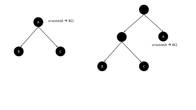
   Figure 3: Converting parse tree so that only leaves have scores.

   We add dummy nodes to the original parse tree as in Figure 3 so that in the modified tree, scores are only on leaves. Now, we are in identical situation as Section 2.3.1, and the same analysis applies.

5. For a substring $s_{i}^{j}$ if $M(i,j+1)$ does not contain any entry with nonterminal $S$, then we declare $s_{i}^{j}\not\in{\mathcal{L}}(G)$ or equivalently its most likely parse has score $0$. Otherwise, we compute the median estimate $d^{i:j}_{med}$ with respect to $S$, and return $\frac{1}{2^{d^{i:j}_{med}}}$ to convert back to probability of the parsing from its computed score.

The bound of $APPROX\text{-}SCFG$ now follows from Theorem 3.

Theorem 4.

] Given a stochastic context free grammar $(G=({\mathcal{N}},\Sigma,{\mathcal{P}},S),\bf{p})$ and a string $s\in\Sigma^{*}$ and any $\epsilon>0$, there exists an algorithm that runs in $\tilde{O}(|G|^{2}\frac{n^{\omega}}{\epsilon^{4}})$ time and with probability at least $(1-\frac{1}{n})$ returns the followings.

• A parsing $\pi^{\prime}(s)$ such that $|\log{{\sf Pr}\left[\pi^{\prime}(s)\right]}|\geq(1-\epsilon)|\log{{\sf Pr}\left[\pi(s)\right]}|$ where $\pi(s)$ is the most likely parse of $s$.

• For every substring $s_{i}^{j}$ $i,j\in\{1,2,...,n\}$ of $s$, and estimate $e(G,s_{i}^{j})$ such that $(1-\epsilon)|\log{{\sf Pr}\left[\pi(s_{i}^{j})\right]}|\leq e(G,s_{i}^{j})\leq(1+\epsilon)|\log{{\sf Pr}\left[\pi(s_{i}^{j})\right]}|$ where $\pi(s_{i}^{j})$ is the most likely parse of $s_{i}^{j}$.

4 Lower Bound

4.1 Subcubic Reduction of APSP to Language Edit Distance

In this section, we prove Theorem 2. Note that, we only allow insertion as edits. Therefore, given a grammar $G$ and a string $s$, $|s|=n$, we compute $s^{\prime}\in{\mathcal{L}}(G)$ such that $s^{\prime}$ can be obtained from $s$ by minimum number of insertions edits on $s$. If no such $s^{\prime}$ exists in ${\mathcal{L}}(G)$, then the language edit distance $d(s,G)$ is $\infty$.

We first define the output of a language edit distance algorithm rigorously. We use a notion of minimum consistent derivation. This is similar to the notion of consistent derivation used by Lee [26] to establish the lower bound for context free parsing. We need to additionally handle distance during parsing.

Definition 7.

Given a context free grammar $G=({\mathcal{N}},\Sigma,{\mathcal{P}},S)$, and a string $s\in\Sigma^{*}$. A nonterminal $A\in{\mathcal{N}}$ mc-derives (minimally and consistently derives) $s_{i}^{j}$ if and only if the following condition holds:

1) If $A$ derives $s_{i}^{j}$ with a minimum score $l$, implying if $A(s)$ is the set of all strings that $A$ derives, $\min_{s^{\prime}\in A(s)}\{dist_{ed}(s^{\prime},s_{i}^{j})\}=l$, and

2. There is a derivation sequence $S\xRightarrow{\ast}s_{1}^{i-1}As_{j+1}^{n}$.

Definition 8.

A $\mathsf{Lan\text{-}Ed}$ is an algorithm that takes a CFG $G=({\mathcal{N}},\Sigma,{\mathcal{P}},S)$ and a string $s\in\Sigma^{*}$ as input and produces output ${\mathcal{F}}_{G,s}$ that acts as an oracle about distance information as follows: for any $A\in{\mathcal{N}}$

• If $A$ minimally and consistently derives $s_{i}^{j}$ with a minimum score $l$, then ${\mathcal{F}}_{G,s}(A,i,j)=l$

• ${\mathcal{F}}_{G,s}$ answers queries in constant time.

The above definition is weaker than the local alignment problem, because we are maintaining only those distances for substrings from which the full string can be derived. All known algorithms for parsing and language edit distance computation maintain this information, because not computing these intermediate results may lead to failure in parsing the full string, or parsing it with minimum number of edits.

The choice of an oracle instead of a particular data structure keeps open the possibility that time required for $\mathsf{Lan\text{-}Ed}$ may be $o(n^{2})$, which will not be the case if we keep a table like most known parsers. The third condition can be relaxed to take poly-logarithmic time in string and grammar size without much effect.

We reduce distance product computation over $(min,+)$-structure to computing language edit distance with insertion. The subcubic equivalence between distance product computation and all-pairs shortest path [46] then establishes Theorem 2. If we allow different edit costs for different terminals, then we can allow all three edits: insertion, deletion and substitution.

Reduction

We are given two weighted matrix $a$ and $b$ of dimension $m\times m$. We assume weights are all positive integers by scaling and shifting and $M=\max_{i,j}{\Big{(}a(i,j),b(i,j)\Big{)}}$. We produce a grammar $G$ and a string $s$ such that from ${\mathcal{F}}_{G,s}$ one can deduce the matrix $c=a\cdot b$.

Let us take $d=\lceil m^{1/3}\rceil$, and we set $\delta=d+2$. Our universe of terminals is $\Sigma=\{s_{1},s_{2},...,s_{3d+6},x\}$. Our input string $s$ is of length $3\delta$ and is simply $s_{1}s_{2}....s_{d+2}s_{d+3}...s_{2d+4}s_{2d+5}....s_{3d+6}$.

Now consider a matrix index $i$, $1\leq i\leq m\leq d^{3}$. Let

$$f_{1}(i)=\lfloor i/d\rfloor$$

and

$$f_{2}(i)=(i~{}mod~{}d)+2.$$

Hence $f_{1}(i)\in[1,d^{2}]$, and $f_{2}(i)\in[2,d+1]$. From $f_{1}(i)$ and $f_{2}(i)$, we can obtain $i$ uniquely. For notational simplicity we use $i_{1}$ to denote $f_{1}(i)$ and $i_{2}$ to denote $f_{2}(i)$. Note that if we decompose $s$ into three consecutive equal parts of size $d+2$ each, then $i_{2}$, $i_{2}+\delta$ and $i_{2}+2\delta$ belong to first, second and third halves respectively.

We now proceed to create the grammar $G=\{{\mathcal{N}},\Sigma,{\mathcal{P}},S\}$. Start from ${\mathcal{N}}=\{S\}$ and ${\mathcal{P}}=\phi$.

• We create $\lfloor\log{(M+1)}\rfloor$ nonterminals as follows. Let $2^{k}\leq(M+1)<2^{k+1}$, then create $X_{2^{k}},X_{2^{k-1}},...,X_{2},X_{1}$. We add the productions

  $$X\longrightarrow x,~{}~{}X_{2^{i}}\longrightarrow X_{2^{i-1}}X_{2^{i-1}},1\leq i\leq k~{}~{}\text{(X-Rule)}.$$

  Let $\hat{w}=X_{2^{j_{1}}}X_{2^{j_{2}}}...X_{2^{j_{l}}}$ if $w=2^{j_{1}}+2^{j_{2}}+...+2^{j_{l}}$.

• We also add for $1\leq r\leq d$ the nonterminals $Y_{1},Y_{2},...,Y_{r}$. Let $2^{l}\leq r<2^{l+1}$, then create nonterminals $Z_{2^{l}},Z_{2^{l-1}},..,Z_{1}$. Add

  $$Z_{1}\longrightarrow\hat{2M+1},~{}~{}Z_{2^{i}}\longrightarrow Z_{2^{i-1}}Z_{2^{i-1}}1\leq i\leq l~{}~{}\text{(Z-Rule)}.$$

  If $r=2^{j_{1}}+2^{j_{2}}+...+2^{j_{l}}$ add

  $$Y_{r}\longrightarrow Z_{2^{j_{1}}}Z_{2^{j_{2}}}...Z_{2^{j_{l}}}~{}~{}\text{(Y-Rule)}.$$

• We now add nonterminal $W$ and productions to generate arbitrary non-empty substrings from $\Sigma\setminus\{x\}$.

  $$W\longrightarrow s_{l}W|s_{l},~{}~{}l\in[1,3d+6]~{}~{}\text{(W-Rule)}.$$

• We also add nonterminals $W_{i}^{j}$ that generates substring $s_{i}s_{i+1}...s_{j}$.

  $$W_{i}^{j}\longrightarrow s_{i}s_{i+1}...s_{j},~{}~{}i,j\in[1,3d+6]~{}~{}\text{(New-W-Rule)}.$$

• Next, we encode the entries of input matrix $A$ and $B$ in our grammar as follows. We add nonterminals from the sets $A_{p,q},B_{p.q}:1\leq p,q,\leq d^{2}$ and $Y_{r}:1\leq r\leq d$. For each entry $a(i,j)=x$, $b(j,k)=y$, we add the production

  $$A_{i_{1},j_{1}}\longrightarrow Y_{\delta-i_{2}}s_{i_{2}}W_{i_{2}+1}^{j_{2}+\delta-1}\hat{x}s_{j_{2}+\delta}Y_{j_{2}}~{}~{}\text{(A-Rule)},$$

  $$B_{j_{1},k_{1}}\longrightarrow Y_{\delta-j_{2}}s_{j_{2}+\delta+1}W_{j_{2}+\delta+2}^{k_{2}+2\delta-1}\hat{y}s_{k_{2}+2\delta}Y_{k_{2}}~{}~{}\text{(B-Rule)}$$

• We now add nonterminals to combine these consecutive substrings. Add $\{C_{p,q}:1\leq p,q\leq d^{2}\}$ and add productions for all $r$, $1\leq r\leq d^{2}$

  $$C_{p,q}\longrightarrow A_{p,r}B_{r,q}~{}~{}\text{(C-Rule)}$$

• Finally, we add the production for the start symbol $S$ for all $p,q$, $1\leq p,q\leq d^{2}$

  $$S\longrightarrow WC_{p,q}W~{}~{}\text{(S-Rule)}$$

The following crucial lemma suggests that by looking at ${\mathcal{F}}_{G,s}(C_{i_{1},j_{1}},s_{i_{2}}^{j_{2}+2\delta})$ we can derive $c(i,j)$ where $i=(i_{1},i_{2})$ and $(j_{1},j_{2})$. This is precisely because $C_{i_{1},j_{1}}$ must derive all the symbols of $s_{i_{2}}^{j_{2}}$ exactly once–a property ensured by adding $Y\text{-}Rule$s, and encodes $c(i,j)$ as the edit distance using $X\text{-}Rule$s.

Lemma 13.

For $1\leq i,j\leq m$, the entry $c_{i,j}=l$, if and only if $C_{i_{1}j_{1}}$ minimally and consistently derives $s_{i_{2}}^{j_{2}+2\delta}$ with score $l+(2M+1)(2\delta+j_{2}-i_{2})$.

Proof.

Fix $i,j$. We first prove the “only-if” part. So let $c_{i,j}=l$. Then there must exists a $k$ such that $a_{i,k}=z$ and $b_{k,j}=l-z$.

We have the C-Rule $C_{i_{1},j_{1}}=A_{i_{1},k_{1}}B_{k_{1},j_{1}}$. Since $a_{i,k}=z$, we have the $A-Rule$ $A_{i_{1},k_{1}}\longrightarrow Y_{\delta-i_{2}}s_{i_{2}}W_{i_{2}+1}^{k_{2}+\delta-1}\hat{z}s_{k_{2}+\delta}Y_{k_{2}}$ and since $b_{k,j}=l-z$, we have the $B-Rule$ $B_{k_{1},j_{1}}\longrightarrow Y_{\delta-k_{2}}s_{k_{2}+\delta+1}W_{k_{2}+\delta+2}^{j_{2}+2\delta-1}\hat{l-z}s_{j_{2}+2\delta}Y_{j_{2}}$. Finally, since $i_{2}+1<k_{2}+\delta-1$ and $k_{2}+\delta+2\leq j_{2}+2\delta-1$, $W_{i_{2}+1}^{k_{2}+\delta-1}\xRightarrow{\ast}s_{i_{2}+1}^{k_{2}+\delta-1}$ and $W_{k_{2}+\delta+2}^{j_{2}+2\delta-1}\xRightarrow{\ast}s_{k_{2}+\delta+2}^{j_{2}+2\delta}$. All the $x$s generated from $\hat{z}$ and $\hat{(l-z)}$ act as deletion errors which need to be fixed by inserting elements in string $s$. Hence $A_{i_{1},k_{1}}$ derives $s_{i_{2}}^{k_{2}+\delta}$ with score $z+(k_{2}+(\delta-i_{2}))(2M+1)|$ and $B_{k_{1},j_{1}}$ derives $s_{k_{2}+\delta+1}^{j_{2}+2\delta}$ with score $l-z+((\delta-k_{2})+j_{2})(2M+1)$. Therefore, $C_{i_{1},j_{1}}$ derives $s_{i_{2}}^{j_{2}+2\delta}$ with score at most $l+(2\delta+j_{2}-i_{2})(2M+1)$.

Finally, $S\xRightarrow{\ast}s_{1}^{i_{2}-1}C_{i_{1},j_{1}}s_{j_{2}+2\delta+1}^{3\delta+6}$ with score at most $l$, since $i_{2}-1\geq 1$ and $j_{2}+2\delta+1<3\delta+6$, hence $C_{i_{1},j_{1}}$ minimally and consistently derives $s_{i_{2}}^{j_{2}+2\delta}$ with score at most $l+(2\delta+j_{2}-i_{2})(2M+1)$.

Now, let us look at the “if” part and assume $C_{i_{1},j_{1}}$ derives $s_{i_{2}}^{j_{2}+2\delta}$ minimally and consistently with a score $l^{\prime}$. This can only arise through an application of C-Rule $C_{i_{1},j_{1}}\longrightarrow A_{i_{1},k^{\prime}_{1}}B_{k^{\prime}_{1},j_{1}}$ such that $A_{i_{1},k^{\prime}_{1}}$ derives $s_{i^{\prime}_{2}}^{k^{\prime}_{2}+\delta}$ within edit distance (say) $z^{\prime}$ and $B_{k^{\prime}_{1},j_{1}}$ derives $s_{k^{\prime\prime}_{2}+\delta+1}^{j^{\prime}_{2}+2\delta}$ within edit distance $l^{\prime}-z^{\prime}$. Then, we must have the productions $A_{i_{1},k^{\prime}_{1}}\longrightarrow Y_{\delta-i^{\prime}_{2}}s_{i^{\prime}_{2}}W_{i^{\prime}_{2}+1}^{k^{\prime}_{2}+\delta-1}\hat{z^{\prime}}s_{k^{\prime}_{2}+\delta}Y_{k^{\prime}_{2}}$ and $B_{k^{\prime}_{1},j_{1}}\longrightarrow Y_{\delta-k^{\prime\prime}_{2}}s_{k^{\prime\prime}_{2}+\delta+1}W_{k^{\prime\prime}_{2}+\delta+2}^{j^{\prime}_{2}+2\delta-1}\hat{l^{\prime}-z^{\prime}}s_{j^{\prime}_{2}+2\delta}Y_{j^{\prime}_{2}}$.

First, since we allow only deletion errors, it is not possible that $k^{\prime}_{2}<k^{\prime\prime}_{2}$, then edit distance will be $\infty$. Similarly, it is not possible that $i^{\prime}_{2}>i_{2}$ or $j^{\prime}_{2}<j_{2}$.

Therefore, the total edit cost paid is $\left[(\delta-i^{\prime}_{2})+k^{\prime}_{2}+(\delta-k^{\prime\prime}_{2})+j_{2}\right](2M+1)+\alpha$ for some $\alpha\leq 2M$. If $i^{\prime}_{2}>i_{2}$ or $j^{\prime}_{2}<j_{2}$, then the above cost is always higher than the case when $i^{\prime}_{2}=i_{2}$ and $j^{\prime}_{2}=j_{2}$. Hence we must use the productions $A_{i_{1},k^{\prime}_{1}}\longrightarrow Y_{\delta-i_{2}}s_{i_{2}}W_{i_{2}+1}^{k^{\prime}_{2}+\delta-1}\hat{z^{\prime}}s_{k^{\prime}_{2}+\delta}Y_{k^{\prime}_{2}}$ and $B_{k^{\prime}_{1},j_{1}}\longrightarrow Y_{\delta-k^{\prime\prime}_{2}}s_{k^{\prime\prime}_{2}+\delta+1}W_{k^{\prime\prime}_{2}+\delta+2}^{j_{2}+2\delta-1}\hat{l^{\prime}-z^{\prime}}s_{j_{2}+2\delta}Y_{j_{2}}$.

If $k^{\prime}_{2}>k^{\prime\prime}_{2}$, then the total score is $\geq(\delta+1)(2M+1)$ due to the $Y$ rules, which is always higher than the case when $k^{\prime}_{2}=k^{\prime\prime}_{2}$. Therefore, it must happen that $k^{\prime}_{2}=k^{\prime\prime}_{2}$. But this can only happen, if there is a number $k^{\prime}$ such that $f_{1}(k^{\prime})=k^{\prime}_{1}$ and $f_{2}(k^{\prime})=k^{\prime}_{2}$ and $a(i,k^{\prime})=z^{\prime}-[(\delta-i^{\prime}_{2})+k^{\prime}_{2}](2M+1)$ and $b(k^{\prime},j)=l^{\prime}-z^{\prime}-[(\delta-k^{\prime}_{2})+j^{\prime}_{2}](M+1)$, and therefore $c(i,j)\leq l^{\prime}-(2\delta+j^{\prime}_{2}-i^{\prime}_{2})(2M+1)$.

The lemma now follows. ∎

Grammar Size

The total number of nonterminals used in this grammar is $O(d^{4}+d^{2}+\log{M})=O(m^{4/3}+\log{M})$ and the number of productions is $O(m^{2}+d^{6}+d^{2}+\log{M})=O(m^{2}+\log{M})$, where $d^{6}$ term comes from the $C\text{-}Rule$ and $m^{2}$ comes from considering all the entries of $A$ and $B$. If we consider the number of nonterminals involved in each production, then the total size of the grammar is $|G|=O(m^{2}\log{M})$.

Note. The grammar constructed here is not in CNF form, but can easily be transformed into a CNF representation $G^{\prime}$ where the number of productions in $G^{\prime}$ increases at most by a factor of $\log{m}$. This happens because in $G$ there is no $\epsilon$ production or unit productions. For every terminal $s_{j}$ $j=1,2,..,3d+6$, we create a nonterminal, $S_{j}$ and replace their occurrences in productions with the newly created nonterminals. We add the productions $S_{j}\rightarrow s_{j}$ for $j=1,2,..,3d+6$. Finally, for every rule of the form $Q\rightarrow R_{1}R_{2}...R_{s}$, we create $s-1$ rules $Q\rightarrow R_{1}Q_{1}$, $Q_{1}\rightarrow R_{2}Q_{2}$,…, $Q_{s-2}\rightarrow R_{s-1}R_{s}$. Since in $G$, the size of $RHS$ is any production can be at most $\lceil\log{M}\rceil+3$, we get the desired bound. Therefore, the claims in this section equally holds when parsers are restricted to work with CNF grammars.

Time Bound

Lemma 14.

Any language edit distance problem $P$ with mc-derivation having run time $O(T(|G|)t(n))$ on grammars of size $|G|$ and strings of length $n$ can be converted into an algorithm MP to compute distance product on positive-integer weighted $m\times m$ matrix with highest weight $M$ that runs in time $O(max(m^{2}+T(m^{2})t(m^{1/3})\log{M})$. In particular, if P takes $O(|G|n^{3-\epsilon})$ time then that implies an $O(m^{3-\epsilon/3}\log{M})$ running time for MP.

Proof.

Given the two matrices $A$ and $B$ of dimension $m\times m$ with maximum weight (after shifting and scaling) $M$, time to read the entries is $O(m^{2})$ and to create grammar $G$ is $O(|G|)=O(m^{2}+m^{4/3}\log{M})$ (note that $d=\lfloor m^{1/3}\rfloor$) and string $s$ is $O(m^{1/3})$. Assume, the parser takes time $O(T_{1}(G)+T_{2}(G)t(n))$ to create ${\mathcal{F}}_{G,s}$. Then we query $\cal{F}_{G,s}$ for each $c_{i,j}$ by creating the query $(C_{i_{1},j_{1}},s_{i_{2}}^{j_{2}+2\delta})$. If the answer is $K$, we set $c_{i,j}=K$. By Lemma 13, the computed value of $c_{i,j}=\min_{k}(a_{i,k}+b_{k,j})$ is correct. Hence once parsing has been done, creating $C$ again takes $O(m^{2})$ time, assuming each query needs $O(1)$ time.

Suppose $T_{1}(G)=T_{2}(G)=|G|$ and $t(n)=n^{3-\epsilon}$, $0<\epsilon\leq 1$then we get an algorithm to compute distance product in time $O(m^{3-\frac{\epsilon}{3}}\log{M})$. ∎

Now, due to sub-cubic equivalence of distance product computation with APSP, Theorem 2 follows.

Reducing APSP to Stochastic Context Free Parsing

The reduction takes the following steps.

1. Reduce $(\min,\times)$-matrix product where matrix entries are drawn from $\mathbb{R}^{+}$ to stochastic context free grammar parsing, that is show if there exists am $O(|G|n^{3-\epsilon}\max_{p\in{\bf p}}{\log{\frac{1}{p}}})$ algorithm for stochastic context free grammar parsing, then there exists one with running time $\tilde{O}(n^{3-\beta}\log{W})$ for $(\min,\times)$-matrix product over $\mathbb{R}^{+}$, $\epsilon,\beta>0$ where $W$ is the maximum weight of any entry.

2. Next we show if there exists an algorithm with running time $\tilde{O}(n^{3-\beta}\log{W})$ for $(\min,\times)$-matrix product with entries in $(0,W]$, $\beta>0$, then there exists one with running time $\tilde{O}(n^{3-\beta}\log{W})$ for detecting negative weight triangle in a weighted graph with weights ranging in $[-W,W]$.

3. Finally, due to sub-cubic equivalence between minimum weight triangle detection with non-negative weights and APSP [46], the result follows.

Reducing $(\min,\times)$-matrix product with entries in $\mathbb{R}^{+}$ to stochastic context free grammar parsing

This reduction is similar to the previous one used for reducing language edit distance problem to distance product computation. Instead of encoding $a_{i,j}=w$, in the production rules $A\text{-}Rule$ and $B\text{-}Rule$, this is encoded in the probability of the corresponding productions.

Definition 9.

Given a stochastic context free grammar $\{G=({\mathcal{N}},\Sigma,{\mathcal{P}},S),{\bf p}\}$, and a string $s\in\Sigma^{*}$. A nonterminal $A\in{\mathcal{N}}$ c-derives (consistently derives) $s_{i}^{j}$ if and only if the following condition holds:

1. $A$ derives $s_{i}^{j}$

2. There is a derivation sequence $S\xRightarrow{\ast}s_{1}^{i-1}As_{j+1}^{n}$.

Definition 10.

A $Stochastic\text{-}Parsing$ is an algorithm that takes a SCFG $\{G=({\mathcal{N}},\Sigma,{\mathcal{P}},S),{\bf p}\}$ and a string $s\in\Sigma^{*}$ as input and produces output ${\mathcal{F}}_{\{G,{\bf p}\},s}$ that acts as an oracle about distance information as follows: for any $A\in{\mathcal{N}}$

• If $A$ consistently derives $s_{i}^{j}$ with maximum probability $q$, then ${\mathcal{F}}_{\{G,{\bf p}\},s}(A,i,j)=q$

• ${\mathcal{F}}_{\{G,{\bf p}\},s}$ answers queries in constant time.

Creating the Grammar.

We are given two matrices $a$ and $b$ with entries from $\mathbb{R}^{+}$, and want to compute their $(\min,\times)$-product $c=a.b:c_{i,j}=\min_{1\leq k\leq n}(a_{i,k}.b_{k,j}).$

Input string. Let us take $d=\lceil m^{1/3}\rceil$, and we set $\delta=d+2$. Our universe of terminals is $\Sigma=\{s_{1},s_{2},...,s_{3d+6},x\}$. Our input string $s$ is of length $3\delta$ and is simply $s_{1}s_{2}....s_{d+2}s_{d+3}...s_{2d+4}s_{2d+5}....s_{3d+6}$. Grammar construction. Consider a matrix index $i$, $1\leq i\leq m\leq d^{3}$. Let $f_{1}(i)=\lfloor i/d\rfloor$ and $f_{2}(i)=(i~{}mod~{}d)+2$. Hence $f_{1}(i)\in[1,d^{2}]$, and $f_{2}(i)\in[2,d+1]$. We can uniquely obtain $i$ from $f_{1}(i)$ and $f_{2}(i)$. For notational simplicity we use $i_{1}$ to denote $f_{1}(i)$ and $i_{2}$ to denote $f_{2}(i)$. If we decompose $s$ into three consecutive equal parts of size $d+2$ each, then $i_{2}$, $i_{2}+\delta$, and $i_{2}+2\delta$ belong to first, second and third halves respectively. We now create the grammar $(G,{\bf p})=(\{{\mathcal{N}},\Sigma,{\mathcal{P}},S\},{\bf p})$. Start from ${\mathcal{N}}=\{S\}$ and ${\mathcal{P}}=\phi$.

• We add nonterminal $W$ and productions to generate arbitrary non-empty substrings from $\Sigma\setminus\{x\}$. $W\longrightarrow s_{l}W|s_{l},~{}l\in[1,3d+6]\text{ each rule having probability }\frac{1}{2(3d+6)}~{}~{}\text{(W-Rule)}.$ The probabilities add up to $1$.

• We encode the entries of $A$ and $B$ in our grammar. We add nonterminals $A_{p,q}:1\leq p,q,\leq d^{2}$, and $B_{p,q}:1\leq p,q\leq d^{2}$. Let $Count_{A}(i_{1},j_{1})=\sum_{i,j:x=f_{1}(i),y=f_{1}(j)}\frac{1}{a_{i,j}}$, and $Count_{B}(i_{1},j_{1})=\sum_{i,j:x=f_{1}(i),y=f_{1}(j)}\frac{1}{b_{i,j}}$. Set $MaxCount_{A}=\max_{x,y,1\leq x,y\leq d^{2}}Count_{A}(i_{1},j_{1})$, and $MaxCount_{B}=\max_{x,y,1\leq x,y\leq d^{2}}Count_{B}(i_{1},j_{1})$. For each entry $a_{i,j},b_{i,j}$, $i=(i_{1},i_{2})$, and $j=(j_{1},j_{2})$ add productions (A-Rule): $A_{i_{1},j_{1}}\longrightarrow s_{i_{2}}Ws_{j_{2}+\delta}\text{ with prob. $\frac{1}{a_{i,j}MaxCount_{A}}$},$ if $MaxCount_{A}>Count_{A}(i_{1},j_{1})$, then add a dummy rule $A_{i_{1},j_{1}}\longrightarrow x\text{ with prob. $\frac{MaxCount_{A}-Count_{A}(i_{1},j_{1})}{MaxCount_{A}}$}.$ Add productions (B-Rule) by replacing every “A” and “a” in (A-Rule) with “B” and “b” respectively.

• We add nonterminals $\{C_{p,q}:1\leq p,q\leq d^{2}\}$ and the productions for all $r$, $1\leq r\leq d^{2}$ $C_{p,q}\longrightarrow A_{p,r}B_{r,q}\text{ with prob. $\frac{1}{d^{2}}$}~{}~{}\text{(C-Rule)}$

• Finally, we add the production for the start symbol $S$ for all $p,q$, $1\leq p,q\leq d^{2}$ $S\longrightarrow WC_{p,q}W\text{ with prob. $\frac{1}{d^{4}}$}~{}~{}\text{(S-Rule)}$

It can be verified that probabilities of all rules with same nonterminal on the LHS add up to $1$. Hence the constructed grammar is a SCFG. The following lemma suggests that by looking at ${\mathcal{F}}_{G,s}(C_{i_{1},j_{1}},s_{i_{2}}^{j_{2}+2\delta})$ we can derive $c(i,j)$ where $i=(i_{1},i_{2})$ and $(j_{1},j_{2})$. Then noting that the grammar size is $O(m^{2})$, and string length $O(m^{1/3})$, we get the desired subcubic equivalence between SCFG parsing and $(\min,\times)$ matrix product (Lemma 16). Note that this non-CNF grammar can easily be converted into a CNF representation with constant factor blow-up in size.

Lemma 15.

For $1\leq i,j\leq m$, the entry $c_{i,j}=l$, if and only if $C_{i_{1}j_{1}}$ $c$-derives $s_{i_{2}}^{j_{2}+2\delta}$ with probability $\frac{1}{ld^{2}.MaxCount_{A}.MaxCount_{B}[2(3d+6)]^{j_{2}+2\delta-i_{2}-2}}$

Proof.

The proof is similar to Lemma 13 instead of computing the total edit distance, compute the total probability of the productions applied to parse $s_{i_{2}}^{j_{2}+2\delta}$.

Fix $i,j$. We first prove the “only-if” part. So let $c_{i,j}=l$. Then there must exists a $k$ such that $a_{i,k}=z$ and $b_{k,j}=\frac{l}{z}$.

We have the C-Rule $C_{i_{1},j_{1}}=A_{i_{1},k_{1}}B_{k_{1},j_{1}}$ with probability $\frac{1}{d^{2}}$. Since $a_{i,k}=z$, we have the (A-Rule) $A_{i_{1},k_{1}}\longrightarrow s_{i_{2}}Ws_{k_{2}+\delta}$ with probability $\frac{1}{zMaxCount_{A}}$and since $b_{k,j}=\frac{l}{z}$, we have the (B-Rule) $B_{k_{1},j_{1}}\longrightarrow s_{k_{2}+\delta+1}Ws_{j_{2}+2\delta}$ with probability $\frac{z}{lMaxCount_{B}}$ . Finally, since $i_{2}+1<k_{2}+\delta-1$ and $k_{2}+\delta+2\leq j_{2}+2\delta-1$, $W\xRightarrow{\ast}s_{i_{2}+1}^{k_{2}+\delta-1}$ with probability $\frac{1}{[2(3d+6)]^{k_{2}+\delta-i_{2}-1}}$ and $W\xRightarrow{\ast}s_{k_{2}+\delta+2}^{j_{2}+2\delta}$ with probability $\frac{1}{[2(3d+6)]^{j_{2}+2\delta-k_{2}-\delta-1}}$. Hence $C_{i_{1},j_{1}}$ derives $s_{i_{2}}^{j_{2}+2\delta}$ with probability at least $\frac{1}{d^{2}}\frac{1}{zMaxCount_{A}}\frac{z}{lMaxCount_{B}}\frac{1}{[2(3d+6)]^{k_{2}+\delta-i_{2}-1+j_{2}+2\delta-k_{2}-\delta-1}}=\frac{1}{d^{2}}\frac{1}{lMaxCount_{A}MaxCount_{B}}\frac{1}{[2(3d+6)]^{j_{2}+2\delta-i_{2}-2}}$.

Finally, $S\xRightarrow{\ast}s_{1}^{i_{2}-1}C_{i_{1},j_{1}}s_{j_{2}+2\delta+1}^{3\delta+6}$ with probability $\frac{1}{d^{4}}$, since $i_{2}-1\geq 1$ and $j_{2}+2\delta+1<3\delta+6$, hence $C_{i_{1},j_{1}}$ consistently derives $s_{i_{2}}^{j_{2}+2\delta}$.

Now, let us look at the “if” part and assume $C_{i_{1},j_{1}}$ derives $s_{i_{2}}^{j_{2}+2\delta}$ consistently with a probability $q$. This can only arise through an application of C-Rule $C_{i_{1},j_{1}}\longrightarrow A_{i_{1},k^{\prime}_{1}}B_{k^{\prime}_{1},j_{1}}$ with probability $\frac{1}{d^{2}}$ such that $A_{i_{1},k^{\prime}_{1}}$ derives $s_{i_{2}}^{k_{2}+\delta}$ and $B_{k^{\prime}_{1},j_{1}}$ derives $s_{k_{2}+\delta+1}^{j_{2}+2\delta}$. Then, we must have the productions $A_{i_{1},k^{\prime}_{1}}\longrightarrow s_{i_{2}}Ws_{k_{2}+\delta}$ with probability $\frac{1}{zMaxCount_{A}}$ where $z=a(i,k),i=(i_{1},i_{2}),k=(k^{\prime}_{1},k_{2})$ and $B_{k^{\prime}_{1},j_{1}}\longrightarrow s_{k^{\prime}_{2}+\delta+1}Ws_{j_{2}+2\delta}$ with probability $\frac{1}{z^{\prime}MaxCount_{B}}$ where $z^{\prime}=b(k,j),k=(k^{\prime}_{1},k_{2}),j=(j_{1},j_{2})$. Now considering the probabilities of W-Rules to generate $s_{i_{2}+1}^{k_{2}+\delta}$ and $s_{k^{\prime}_{2}+\delta+2}^{j_{2}+2\delta-1}$, the “if” part is established.

The lemma now follows. ∎

Lemma 16.

Any stochastic context free parsing problem $P$ with c-derivation having run time $O(T(|G|)t(n)\max{\log_{p\in\bf{p}}})$ on grammars of size $|G|$ and strings of length $n$ can be converted into an algorithm MP to compute $(\min,\times)$-product of $m\times m$ matrices with entries in $\mathbb{R}\setminus\{0\}$ with highest weight $M$ that runs in time $\tilde{O}(max(m^{2}+T(m^{2})t(m^{1/3})\log{M})$. In particular, if P takes $O(|G|n^{3-\epsilon}\max{\log_{p\in\bf{p}}\frac{1}{p}})$ time then that implies an $\tilde{O}(m^{3-\epsilon/3}\log{M})$ running time for MP.

Proof.

The proof follows from Lemma 15 and following similar steps as Lemma 14. ∎

From $(min,\times)$-matrix product with positive real entries to Negative Triangle Detection.

we show if there exists an algorithm with running time $\tilde{O}(n^{3-\beta}\log{W})$ for $(\min,\times)$-matrix product with entries in $(0,W]$, $\beta>0$, then there exists one with running time $\tilde{O}(n^{3-\beta}\log{W})$ for detecting negative weight triangle in a weighted graph with weights ranging in $[-W,W]$.

We now show that if there exists an algorithm with running time $\tilde{O}(n^{3-\beta}\log{W})$ for $(\min,\times)$-matrix product over $\mathbb{R}^{+}$ with weights in $(0,W)$, $\beta>0$, then there exists one with running time $\tilde{O}(n^{3-\beta}\log{W})$ to detect if a weighted graph $G=(V,E)$ has a triangle of negative total edge weight where weights are in $[-W,W]$.

We assume all edge weights are integers, and the maximum absolute weight $W$ is at least 3. Both of these can be achieved by appropriately scaling the edge weights.

Let $W$ be the maximum absolute weight on any edge $e\in E$, $|W|\geq 3$. Set $A(i,j)=w_{i,j}+W^{3}$, and $B(i,j)=A(i,j)$. Therefore, all entries of $A$ and $B$ are $>0$. Find the $(\min,\times)$ product of $C=A\bigodot_{\min,\times}B$. Let $C^{\prime}(i,j)=C(i,j)-W^{6}+W^{3}w_{i,j}+2W^{2}$.

If there exists a negative triangle $i\rightarrow k\rightarrow j$, then $w_{i,k}+w_{k,j}+w_{i,j}\leq-1$. Hence $W^{3}(w_{i,k}+w_{k,j}+w_{i,j})\leq-W^{3}$ or, $W^{3}(w_{i,k}+w_{k,j}+w_{i,j})+2W^{2}\leq-W^{3}+2W^{2}\leq-W^{2}$. Now $(w_{i,k}+W^{3})(w_{k,j}+W^{3})=w_{i,k}w_{k,j}+W^{3}(w_{i,k}+w_{k,j})+W^{6}$ Hence, $C^{\prime}(i,j)=\min_{k}(w_{i,k}w_{k,j}+W^{3}(w_{i,k}+w_{k,j}+w_{i,j})+2W^{2}$. Now $-W^{2}\leq w_{i,k}w_{k,j}\leq W^{2}$. Therefore, if there is a negative triangle involving edge $(i,j)$, then $C^{\prime}(i,j)\leq W^{2}+\min_{k}(W^{3}(w_{i,k}+w_{k,j}+w_{i,j})+2W^{2}\leq 0$

On the other hand, if there is no negative triangles, then $C^{\prime}(i,j)\geq-W^{2}+2W^{2}=W^{2}\geq 9$ for all $1\leq i,j\leq n$.

Therefore, there exists a negative triangle in $G$ if and only if there is a negative entry in $C^{\prime}$. While $C$ can be computed in asymptotically same time as computing $(\min,\times)$-matrix product of two $n\times n$ dimensional matrices with real positive entries, $C^{\prime}$ can be computed from $C$ in $O(n^{2})$ time.

Hence, we get the following lemma.

Lemma 17.

Given two $n\times n$ matrices with positive real entries with maximum weight $W$ if their $(\min,\times)$-matrix product can be done in time $O(T(n)\log{W})$ time, then $\tilde{O}([T(n)+n^{2}]\log{W})$ time is sufficient to detect negative triangles on weighted graphs with $n$ vertices and weights in $[-W,W]$.

Now, due to subcubic equivalence between negative triangle detection and APSP, we get the following theorem.

Theorem (1).

Given a stochastic context-free grammar $\{G=({\mathcal{N}},\Sigma,{\mathcal{P}},S),{\bf p}\}$, and a string $s\in\Sigma^{*}$, $|s|=n$, if the SCFG parsing problem can be solved in $O(|G|n^{3-\delta}\max{\log_{p\in\bf{p}}\frac{1}{p}})$ time then that implies an algorithm with running time $\tilde{O}(m^{3-\delta/3}\log{W})$ for all-pairs shortest path problem on weighted digraphs with $m$ vertices and maximum weight $W$.

This leads to the following corollary by sub-cubic equivalence of all-pairs shortest path with many other fundamental problems on graphs and matrices [46, 1].

Corollary 6.

Given a stochastic context-free grammar $\{G=({\mathcal{N}},\Sigma,{\mathcal{P}},S),{\bf p}\}$, and a string $s\in\Sigma^{*}$, $|s|=n$, if the SCFG parsing problem can be solved in $O(|G|n^{3-\delta}\max{\log_{p\in\bf{p}}\frac{1}{p}})$ time then that implies an algorithm with running time $\tilde{O}(m^{3-\delta/3})$, $\gamma,\delta>0$ for all of the following problems.

1. Minimum weight triangle: Given an $n$-node graph with real edge weights, compute $u,v,w$ such that $(u,v),(v,w),(w,u)$ are edges and the sum of edge weights is minimized.

2. Negative weight triangle: Given an $n$-node graph with real edge weights, compute $u,v,w$ such that $(u,v),(v,w),(w,u)$ are edges and the sum of edge weights is negative.

3. Metricity: Determine whether an $n\times n$ matrix over $\mathbb{R}$ defines a metric space on $n$ points.

4. Minimum cycle: Given an $n$-node graph with real positive edge weights, find a cycle of minimum total edge weight.

5. Second shortest paths: Given an $n$-node directed graph with real positive edge weights and two nodes $s$ and $t$, determine the second shortest simple path from $s$ to $t$.

6. Replacement paths: Given an $n$-node directed graph with real positive edge weights and a shortest path $P$ from node $s$ to node $t$, determine for each edge $e\in P$ the shortest path from $s$ to $t$ in the graph with $e$ removed.

7. Radius problem: Given an $n$-node weighted graph with real positive edge weights, determine the minimum distance $r$ such that there is a vertex $v$ with all other vertices within distance $r$ from $v$.

Reducing APSP to Weighted Language Edit Distance Problem

In the weighted language edit distance problem, we are given a context free language ${\mathcal{L}}(G)=({\mathcal{N}},\Sigma,{\mathcal{P}},S)$ and a string $s\in\Sigma^{*}$ along with a scoring function $score:\Sigma\times\{Insertion,Deletion,Substitution\}\rightarrow\mathbb{R}^{+}$, the goal is to do minimum total weighted edits on $s$ according to the scoring function to map it to ${\mathcal{L}}(G)$.

To reduce APSP to weighted language edit distance problem, we use the same construction used to prove Theorem 2, and in addition we define a scoring function. For insertion edits, all terminals in $\Sigma$ get a score of $1$. However, for deletion and substitution, we set for every $x\in\Sigma$, $score(x,deletion)=score(x,substitution)=(3d+6)(M+1)$. Deletion or substitution of any element in the input string $s$ is too costly. An optimum algorithm for the weighted language edit distance will therefore never do deletion or substitution. The entire analysis of Theorem 2 now applies.

5 Conclusion

In this paper, we make significant progress on the state-of-art of stochastic context free grammar parsing, and language edit distance problem. Context free grammars are the pillar of formal language theory. Grammar based distance computation and stochastic grammars have been proven to be very powerful tools with huge applications. Here, we give the the first sub-cubic algorithms with running time $\tilde{O}(\frac{n^{\omega}}{\epsilon})$ for both of these problems that return near-optimal results.

For the first time, we lay out their connections to fundamental problems on graphs and matrices, and show that improvement in the exact computation of either SCFG parsing or language edit distance computation will lead to major breakthroughs in a large variety of problems.

Many questions remain. Understanding the general relationship between parsing time and language edit distance computation is a big open problem. Allowing additive approximation may break the barrier of $n^{\omega}$ in running time. We have initial results that suggest in this direction.

Acknowledgement. The author thanks Alfred Aho for asking whether language edit distance can be cast as an algebraic closure over a closed semiring, and anonymous reviewers for pointing out a glitch in the construction of Sidon sequence and for many helpful comments. The author also thanks Karl Bringmann for subsequent discussions on this problem, and for pointing out that using substitution in the lower bound proof is problematic.

6 Appendix

Keeping Parsing Information.

Parsing information can be kept easily. Suppose $(A_{x},u)\in M(i,j)$ and $(A_{y},v)\in M(j,k)$. Now maintain with $(A_{x},u)$, the start and end point of substring that it generates. So we maintain $(A_{x},u,i,j-1)$. Similarly for $(A_{y},v)$ we instead maintain $(A_{y},v,j,k-1)$. Now if $B\rightarrow A_{x}A_{y}$ is a production, and we include $(B,u+v,i,k-1)$ in $M(i,k)$ we also maintain the production that gave rise to this entry. Hence, overall we maintain at $M(i,k)$ the entry $\{(B,u+v,i,k-1),(B,u+v,i,k-1)\rightarrow(A_{x},u,i,j-1)(A_{y},v,j,k-1)$.

To obtain parsing information for any string $s_{i}^{k}$, we consider $M(i,k+1)$ and look for the entry that involves the start symbol $S$. If the retrieved entry is $\{(S,z,i,k),(S,z,i,k)\rightarrow(A_{x},u,i,j-1)(A_{y},v,j,k)$. Then, we include $S\rightarrow A_{x}A_{y}$ as the first derivation applied for parsing. We then look for the entry with $A_{x}$ in $M(i,j)$ and the entry for $A_{y}$ in $M(j,k+1)$, and proceed recursively to obtain the full parsing information. The total number of cells of $M$ that we need to look up is $O(k-i)$, and hence the full parsing information for $s_{i}^{k}$ can be obtained in $O(k-i)$ time.

References

- [1] Amir Abboud, Virginia Vassilevska Williams, and Oren Weimann. Consequences of faster alignment of sequences. ICALP, pages 39–51, 2014.
- [2] Alfred V. Aho and John E. Hopcroft. The Design and Analysis of Computer Algorithms. Addison-Wesley Longman Publishing Co., Inc., Boston, MA, USA, 1st edition, 1974.
- [3] Alfred V. Aho and Thomas G. Peterson. A minimum distance error-correcting parser for context-free languages. SIAM J. Comput., 1(4), 1972.
- [4] Tatsuya Akutsu. Approximation and exact algorithms for RNA secondary structure prediction and recognition of stochastic context-free languages. Journal of Combinatorial Optimization, 3(2-3).
- [5] Noga Alon, Zvi Galil, and Oded Margalit. On the exponent of the all pairs shortest path problem. J. Comput. Syst. Sci., 54(2), April 1997.
- [6] Noga Alon, Michael Krivelevich, Ilan Newman, and Mario Szegedy. Regular languages are testable with a constant number of queries. SIAM J. Comput., 30(6), December 2001.
- [7] Alexandr Andoni, Robert Krauthgamer, and Krzysztof Onak. Polylogarithmic approximation for edit distance and the asymmetric query complexity. FOCS, 2010.
- [8] Alexandr Andoni and Krzysztof Onak. Approximating edit distance in near-linear time. STOC, 2009.
- [9] Arturs Backurs and Piotr Indyk. Edit distance cannot be computed in strongly subquadratic time (unless SETH is false). STOC, 2015.
- [10] Ziv Bar-Yossef, T. S. Jayram, Robert Krauthgamer, and Ravi Kumar. Approximating edit distance efficiently. FOCS, 2004.
- [11] Tuğkan Batu, Funda Ergun, and Cenk Sahinalp. Oblivious string embeddings and edit distance approximations. SODA, 2006.
- [12] Amit Chakrabarti, Graham Cormode, Ranganath Kondapally, and Andrew McGregor. Information cost tradeoffs for augmented index and streaming language recognition. FOCS, 2010.
- [13] Richard Cole and Ramesh Hariharan. Approximate string matching: A simpler faster algorithm. SIAM J. Comput., 31(6), June 2002.
- [14] Richard Durbin. Biological sequence analysis: probabilistic models of proteins and nucleic acids. Cambridge university press, 1998.
- [15] P Erdös and Pál Turán. On a problem of Sidon in additive number theory, and on some related problems. Journal of the London Mathematical Society, 1(4).
- [16] Steven Grijzenhout and Maarten Marx. The quality of the XML web. Web Semant., 19, 2013.
- [17] Dan Gusfield. Algorithms on Strings, Trees, and Sequences: Computer Science and Computational Biology. Cambridge University Press, New York, NY, USA, 1997.
- [18] R.R Gutell, J.J. Cannone, Z Shang, Y Du, and M.J Serra. A story: unpaired adenosine bases in ribosomal RNAs. Journal of Mol Biology, 2010.
- [19] Yuri A. Ivanov and Aaron F. Bobick. Recognition of visual activities and interactions by stochastic parsing. IEEE Transactions on Pattern Analysis and Machine Intelligence, 22(8), 2000.
- [20] Mark Johnson. PCFGs, Topic Models, Adaptor Grammars and Learning Topical Collocations and the Structure of Proper Names. ACL, 2010.
- [21] Donald E. Knuth. The Art of Computer Programming, Volume 2 (3rd Ed.): Seminumerical Algorithms. 1997.
- [22] Flip Korn, Barna Saha, Divesh Srivastava, and Shanshan Ying. On repairing structural problems in semi-structured data. VLDB, 2013.
- [23] Andreas Krebs, Nutan Limaye, and Srikanth Srinivasan. Streaming algorithms for recognizing nearly well-parenthesized expressions. MFCS, 2011.
- [24] Gad M. Landau, Eugene W. Myers, and Jeanette P. Schmidt. Incremental string comparison. SIAM J. Comput., 27(2), April 1998.
- [25] François Le Gall. Faster algorithms for rectangular matrix multiplication. FOCS, 2012.
- [26] Lillian Lee. Fast context-free grammar parsing requires fast boolean matrix multiplication. J. ACM, 49(1), January 2002.
- [27] Frédéric Magniez, Claire Mathieu, and Ashwin Nayak. Recognizing well-parenthesized expressions in the streaming model. STOC, 2010.
- [28] Michael I Miller and Joseph A O’Sullivan. Entropies and combinatorics of random branching processes and context-free languages. IEEE Transactions on Information Theory,, 38(4), 1992.
- [29] Darnell Moore and Irfan Essa. Recognizing multitasked activities from video using stochastic context-free grammar. NCAI, 2002.
- [30] Gene Myers. Approximately matching context-free languages. Information Processing Letters, 54, 1995.
- [31] Kevin O’Bryant. A complete annotated bibliography of work related to Sidon sequences. Electron. J. Combin., 575, 2004.
- [32] Michal Parnas, Dana Ron, and Ronitt Rubinfeld. Testing membership in parenthesis languages. Random Struct. Algorithms, 22(1), January 2003.
- [33] Geoffrey K Pullum and Gerald Gazdar. Natural languages and context-free languages. Linguistics and Philosophy, 4(4), 1982.
- [34] Sanguthevar Rajasekaran and Marius Nicolae. An error correcting parser for context free grammars that takes less than cubic time. Manuscript, 2014.
- [35] Andrea Rosani, Nicola Conci, and Francesco G. De Natale. Human behavior recognition using a context-free grammar. Journal of Electronic Imaging.
- [36] Imre Z Ruzsa. An infinite Sidon sequence. Journal of Number Theory, 68(1), 1998.
- [37] Barna Saha. The Dyck language edit distance problem in near-linear time. FOCS, 2014.
- [38] S. C. Sahinalp and U. Vishkin. Efficient approximate and dynamic matching of patterns using a labeling paradigm. FOCS, 1996.
- [39] Yasubumi Sakakibara. Grammatical inference in bioinformatics. Pattern Analysis and Machine Intelligence, IEEE Transactions on, 27(7), 2005.
- [40] Tadao Takaoka. Subcubic cost algorithms for the all pairs shortest path problem. Algorithmica, 20(3), 1998.
- [41] Leslie G Valiant. General context-free recognition in less than cubic time. Journal of computer and system sciences, 10(2), 1975.
- [42] Balaji Venkatachalam, Dan Gusfield, and Yelena Frid. Faster algorithms for RNA-folding using the four-russians method. WABI, 2013.
- [43] Milind Mahajan Wang, Ye-Yi and Xuedong Huang. A unified context-free grammar and n-gram model for spoken language processing. ICASP, 2000.
- [44] Ryan Williams. Faster all-pairs shortest paths via circuit complexity. STOC, 2014.
- [45] Virginia Vassilevska Williams. Multiplying matrices faster than coppersmith-winograd. STOC, 2012.
- [46] Virginia Vassilevska Williams and Ryan Williams. Subcubic equivalences between path, matrix and triangle problems. FOCS, 2010.
- [47] Raphael Yuster. Efficient algorithms on sets of permutations, dominance, and real-weighted APSP. SODA, 2009.
- [48] Shay Zakov, Dekel Tsur, and Michal Ziv-Ukelson. Reducing the worst case running times of a family of RNA and CFG problems, using Valiant’s approach. WABI, 2010.
- [49] Weiling Zhu and Javier Garcia-Frias. Stochastic context-free grammars and hidden Markov models for modeling of bursty channels. IEEE Transactions on Vehicular Technology, 53(3), 2004.
- [50] Uri Zwick. All pairs shortest paths in weighted directed graphs–exact and almost exact algorithms. FOCS, 1998.