Abstract

In this article we study weak gravitational lensing of regular Bardeen black hole which has scalar charge $g$ and mass $m.$ We investigate the angular position and magnification of non-relativistic images in two cases depending on the presence or absence of photon sphere. Defining dimensionless charge parameter $q=\frac{g}{2m}$ we seek to disappear photon sphere in the case of $|q|>{24\sqrt{5}}/{125}$ for which the space time metric encounters strongly with naked singularities. We specify the basic parameters of lensing in terms of scalar charge by using the perturbative method and found that the parity of images is different in two cases: (a) The strongly naked singularities is present in the space time. (b) singularity of space time is weak or is eliminated (the black hole lens).

1 Introduction

When the light ray passes from the vicinity of a massive object it is deflected because of the interaction between light and gravitational field of the massive object. So each massive object can act like a lens and causes a phenomena called gravitational lensing. Depending on the amount of light deflection, the gravitational lensing is divided to weak and strong ranges. Weak deflection limit occurs when light ray passes far away from the photon sphere whereas strong deflection limit occurs when light ray passes from the vicinity of the photon sphere. In the latter case it may turn around the lens once or more and relativistic images are formed. Light rays which pass from the inside of the photon sphere cannot escape from the gravitational field of lens, so no images can be created. Many articles have investigated gravitational lensing by using analytical approach in the weak [1-7] and strong [8-17] deflection limits. Besides, numerical methods is also used to study the gravitational lensing of black holes and naked singularities [18-23]. Furthermore different approaches such as Amore et. al [24,25] and Ayer et. al [26] in the study of gravitational lensing are presented. Gravitational lensing is a powerful observational tool for probing black holes at the center of galaxies. In article [27] different approaches of gravitational lensing along with observational prospects are reviewed. Cosmological and black hole solutions which cause to make singularities in general relativity are important subject because of the divergence of curvature. Regular black holes are metric solutions which contain horizons but without singularities. The first regular black hole (RBH) which is introduced by Bardeen [28], has both event and Cauchy horizons, but with a regular center. Borde showed [29-30] that the absence of the singularity is related to topology change in de-Sitter like core. Bardeen black hole is spherically symmetric static solution of the Einstein field equations coupled to a nonlinear electrodynamics source [31] containing two characteristics namely charge g and mass m. Gravitational lensing of the regular Bardeen black hole was studied in the strong deflection limit by Eiroa and Sendra [17]. They used Bozza method [9] to calculate deflection angle for small values of scalar charge $|q|<q_{ph}$ where $q_{ph}=\frac{24\sqrt{5}}{125}\approx 0.43$ and obtained the positions and magnifications of the relativistic images. They also applied the results to a supermassive black hole located at the center of assumed Galaxy.
In this paper we have studied gravitational lensing of Bardeen metric in weak deflection limit in cases where the lens treats as black hole and naked singularities. We use perturbation approach presented by Keeton et. al [5] and find positions of primary and secondary non-relativistic images. We should point that all image angular positions are re-scaled to angular Einstein radius ($\vartheta_{E}$) throughout this paper. Organization of the paper is given as follows.
In section 2 we define the Bardeen black hole metric. We specify Taylor series expansion of the elliptical integral of deflection angle of light ray in terms of the inverse of dimensionless impact parameter $u=\frac{b}{2m}=\frac{1}{2m}\left|\frac{L}{E}\right|>1$ where $m$, $L$ and $E$ are the mass of gravitational lens, the constant angular momentum and the energy of light ray respectively. We also identify the locations of the horizons and the photon sphere of the Bardeen black hole (lens). In section 3 we use Virbhadra-Ellis lens equation [21] and find its Taylor series expansion in terms of $u$. Then we determine the non-relativistic image positions. In section 4 we obtain the magnification of the images by using Taylor series expansion of the magnification equation. Total and weighted-centroid magnifications are also evaluated. In section 5 we discuss results of the our work.

2 Bardeen black holes and deflection angle

Regular black holes, are the solutions of the gravity equations for which an event horizon exist, although there is no singularity. Usually they are supported by nonlinear electromagnetic fields and so they have at least two characteristics namely mass $m$ and charge $g$ [28,32]. They are good candidates for the supper-massive Galactic black holes treated as particle accelerators [33]. The first RBH metric was introduced by Bardeen as follows

$$ds^{2}=-A(r)dt^{2}+B(r)dr^{2}+C(r)(d\theta^{2}+\sin^{2}\theta d\varphi^{2})$$ (2.1)

where

$$A(r)=1-\frac{2mr^{2}}{\big{(}r^{2}+g^{2}\big{)}^{3/2}}\;,\;B(r)=\frac{1}{A(r)}\;,\;C(r)=r^{2}$$ (2.2)

It can be interpreted as a magnetic solution of the Einstein equations coupled to nonlinear electrodynamics [31]. Its Ricci and Kretchmann scalars are calculated as

$$R^{\mu}_{\mu}={\frac{6m{g}^{2}\left(4\,{g}^{2}-{r}^{2}\right)}{\left({r}^{2}+{g}^{2}\right)^{7/2}}}$$ (2.3)

and

$$R_{\mu\nu\eta\lambda}R^{\mu\nu\eta\lambda}={\frac{{12m}^{2}\left(4\,{r}^{8}-12\,{g}^{2}{r}^{6}+47\,{g}^{4}{r}^{4}-4\,{g}^{6}{r}^{2}+8\,{g}^{8}\right)}{\left({r}^{2}+{g}^{2}\right)^{7}}}$$ (2.4)

which have regular values in all points of the space-time for $g\neq 0.$ The above black hole metric reduces to de-Sitter like space-time in small $r$. Defining a dimensionless parameter called scalar charge as

$$q=\frac{g}{2m}$$ (2.5)

one can obtain that the Bardeen black hole reduces to Schwarzschild space-time for $q=0$ and also for in regions with large $r$ (in the case of $q\neq 0$). Its horizons disappear for $|q|>q_{h}$ where $q_{h}=\frac{2\sqrt{3}}{9}\approx 0.38$ and its photon sphere also disappears for $|q|<q_{ph}$ ($q_{ph}=\frac{24\sqrt{5}}{125}\approx 0.43$), so that we have three cases in study of gravitational lensing: (i) Regular black hole (RBH) in case $|q|<q_{h}.$ (ii) weakly naked singularity (WNS) in case $q_{h}<|q|<q_{ph}.$ (iii) strongly naked singularity (SNS) in case $|q|>q_{ph}$.
It is convenient to use dimensionless elements of the metric as

$$dS^{2}=(2m)^{-2}ds^{2}=-A(x)dT^{2}+B(x)dx^{2}+C(x)d\Omega^{2}$$ (2.6)

where we define

$$x=\frac{r}{2m}~{},~{}T=\frac{t}{2m}$$ (2.7)

and

$$A(x)=B(x)^{-1}=1-\frac{x^{2}}{\big{(}x^{2}+q^{2}\big{)}^{3/2}}\;,\;C(x)=x^{2}.$$ (2.8)

We can determine locations of the apparent and event horizons of the Bardeen black hole $x_{h}$ by solving the equation $A(x_{h})=0$ as

$$x_{h}^{6}+(3q^{2}-1)x_{h}^{4}+3q^{4}x_{h}^{2}+q^{6}=0~{}.$$ (2.9)

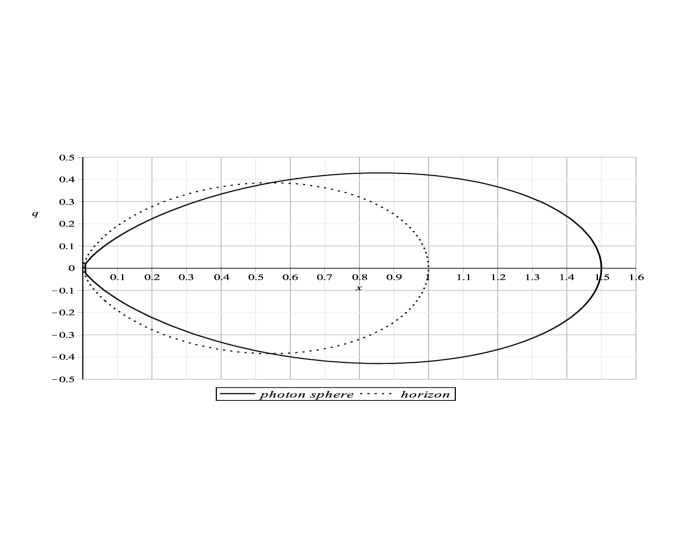
Figure 1:  Diagram of the horizon (dotted-line) and photon sphere radiuses (solid-line) are plotted against dimensionless scalar charge $q.$

Diagram of the above equation is plotted against $q$ in figure 1 (dotted line).
The photon sphere radius $x_{ps}$ is given by the largest positive solution of the following equation [34] (see also Eq. 29 in Ref. [27]).

$$\frac{C^{\prime}(x_{ps})}{C(x_{ps})}=\frac{A^{\prime}(x_{ps})}{A(x_{ps})}$$ (2.10)

where the prime denotes differentiation with respect to $x$. Inserting (2.8) into (2.10), this equation leads to

$$4(x_{ps}^{2}+q^{2})^{5}-9x_{ps}^{8}=0~{}.$$ (2.11)

Diagram of the above equation is plotted against $q$ in figure 1 (solid line).
Deflection angle of light ray coming from infinity is specified by solving the geodesic equation as

$$\alpha(r_{0})=2\Delta\phi(r_{0})-\pi$$ (2.12)

where $r_{0}>r_{ps}$ is closest approach distance of the light ray from center of the Bardeen black hole. Also we have [27]:

$$\Delta\phi(r_{0})=b\int_{r_{0}}^{\infty}\Bigg{(}\frac{B(r)}{C(r)}\Bigg{)}^{1/2}\Bigg{(}\frac{C(r)}{A(r)}-b^{2}\Bigg{)}^{-1/2}dr$$ (2.13)

in which impact parameter b is defined as

$$b=\sqrt{\frac{C(r_{0})}{A(r_{0})}}~{}.$$ (2.14)

Applying (2.7) and (2.8), the equations defined by (2.13) and (2.14) lead to the following forms respectively

$$\Delta\phi(x_{0})=\int_{x_{0}}^{\infty}\frac{x_{0}dx}{x\sqrt{x^{2}\bigg{(}1-\frac{x_{0}^{2}}{\big{(}x_{0}^{2}+q^{2}\big{)}^{3/2}}\bigg{)}-x_{0}^{2}\bigg{(}1-\frac{x^{2}}{\big{(}x^{2}+q^{2}\big{)}^{3/2}}\bigg{)}}}$$ (2.15)

and

$$\frac{b}{2m}=\frac{x_{0}}{\sqrt{1-x_{0}^{2}/(x_{0}^{2}+q^{2})^{3/2}}}~{}.$$ (2.16)

Using the transformation $z=\frac{x_{0}}{x},$ the equation (2.15) can be rewritten as follows.

$$\Delta\phi(x_{0})=\int_{0}^{1}\frac{dz}{\sqrt{1-\frac{x_{0}^{2}}{\big{(}x_{0}^{2}+q^{2}\big{)}^{3/2}}-z^{2}+\frac{x_{0}^{2}z^{3}}{\Big{(}x_{0}^{2}+q^{2}z^{2}\Big{)}^{3/2}}}}$$ (2.17)

which diverges to infinity at $z=1$. If we want to evaluate (2.17) in limits of weak gravitational lensing where $x_{0}>>1$, we must be find its Taylor series expansion about $\frac{1}{x_{0}}$ and integrate it term by term as follows.

$$\alpha(x_{0})=\frac{2}{x_{0}}+\Big{(}\frac{15\pi}{16}-1\Big{)}\frac{1}{x^{2}_{0}}+\Big{(}\frac{61}{12}-\frac{15\pi}{16}-4q^{2}\Big{)}\frac{1}{x_{0}^{3}}+$$

$$\bigg{(}\frac{3465\pi}{1024}-\frac{65}{8}+\Big{(}\frac{15}{2}-\frac{315\pi}{64}\Big{)}q^{2}\bigg{)}\frac{1}{x^{4}_{0}}+$$

$$\bigg{(}\frac{7783}{320}-\frac{3465\pi}{512}+\big{(}\frac{90\pi}{8}-\frac{195}{4}\big{)}q^{2}+6q^{4}\bigg{)}\frac{1}{x^{5}_{0}}+O\bigg{(}\frac{1}{x_{0}^{6}}\bigg{)}~{}.$$ (2.18)

The above convergent series expansion is described in terms of closest distance $x_{0}>1$ which it is coordinate dependent. But we should rewrite (2.18) against coordinate invariant expression such as impact parameter of the light ray $b=\left|\frac{L}{E}\right|.$ This is a good candidate for our purpose where $L$ and $E$ are the constants of angular momentum and energy of the light ray respectively [35]. This constant like the black hole mass $m$ and charge $g$ is invariant so the above expansion series described in terms of $b$ is coordinate-free. Furthermore we should note that in the weak gravitational lensing approach we must set $m/b<<1$ which is equivalent to $x_{0}>>1.$ Therefore we need Taylor series expansion of the function $x_{0}(b)$ obtained from (2.16) as follow.

$$\frac{1}{x_{0}}=\frac{2m}{b}+\frac{1}{2}\Big{(}\frac{2m}{b}\Big{)}^{2}+\frac{5}{8}\Big{(}\frac{2m}{b}\Big{)}^{3}+(2-\frac{3}{2}q^{2})\Big{(}\frac{2m}{b}\Big{)}^{4}+\Big{(}\frac{231}{64}-\frac{21}{4}q^{2}\Big{)}\Big{(}\frac{2m}{b}\Big{)}^{5}+\cdots.$$ (2.19)

Substituting (2.19) the equation (2.18) become

$$\alpha_{q}(u>1)=\frac{A_{1}}{u}+\frac{A_{2}}{u^{2}}+\frac{A_{3}}{u^{3}}+\frac{A_{4}}{u^{4}}+\frac{A_{5}}{u^{5}}+\cdots$$ (2.20)

where $u=\frac{b}{2m}$ is dimensionless impact parameter and

$$A_{1}=2\;\;,A_{2}=\frac{15\pi}{16}\;\;,A_{3}=\frac{4}{3}\big{(}4-3q^{2}\big{)}\;\;,A_{4}=\frac{315\pi}{1024}\big{(}11-16q^{2}\big{)},$$

$$A_{5}=\frac{2}{5}\big{(}56-120q^{2}+15q^{4}\big{)}~{}.$$ (2.21)

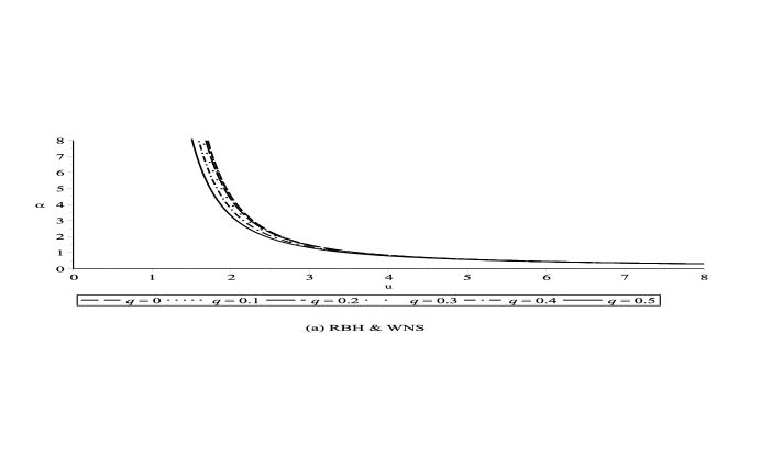
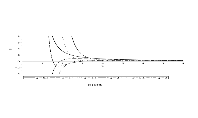
Figure 2:  Diagram of deflection angle $\alpha$ is plotted against dimensionless impact parameter $u$.

The Taylor series expansion (2.20) remains convergent for $u>\sqrt[n]{A_{n}}$ $;n=1,2,3,\cdots$ even if we choose large scalar charge values ($|q|>q_{ph}$) i.e. for SNS. Diagram of the deflection angle equation (2.20) is plotted against $u$ for different values of scalar charge $q$ in figure 2. Figure 2-a shows that for RBH and WNS with fixed $|q|$, the deflection angle decreases with respect to impact parameter whereas in case of SNS, there are some values of q for which the diagram is not treat monotonously. We should note that the relativistic images are formed when $\alpha\geq\frac{3\pi}{2}\approx 4.71.$ We focus here on non-relativistic images for which diagrams in figure 2 are only valid for $\alpha<4.71~{}.$

3 Lens equation and Image positions

We take Virbhadra-Ellis lens equation [21] as

$$tan\mathfrak{B}=tan\vartheta-D(tan\vartheta+tan(\alpha-\vartheta))$$ (3.1)

where $\mathfrak{B}$ and $\vartheta$ are source and image angular positions measured from the optical axis respectively, and D is defined as

$$D=\frac{d_{ls}}{d_{os}}$$ (3.2)

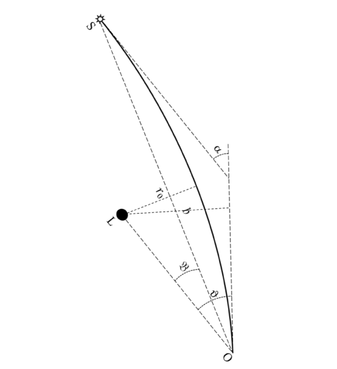
Figure 3:  Gravitational lensing configuration. $\alpha$, b and $r_{0}$ are respectively deflection angle, impact parameter and closest approach distance of the light ray. $\mathfrak{B}$ and $\vartheta$ are the angular positions of source and image measured from the optical axis. Position of the source, the lens and the observer are called by S, L and O.

where $d_{ls}$ and $d_{os}$ are source-lens and source-observer distance respectively (see figure 3). One of important quantities in study of the gravitational lensing is angular radius of Einstein rings

$$\vartheta_{E}=\sqrt{\frac{4GmD}{c^{2}d_{ol}}}$$ (3.3)

where $G$, $c$, $m$ and $d_{ol}$ are Newton‘s gravitational constant, speed of light, lens mass and lens-observer distance respectively. Now, we define re-scaled angular parameters as

$$\beta=\frac{\mathfrak{B}}{\vartheta_{E}}~{},~{}\theta=\frac{\vartheta}{\vartheta_{E}}~{}.$$ (3.4)

According to the postulate presented by Keeton [35], solutions of the lens equation (3.1) are assumed to be have Taylor series expansion as

$$\theta=\theta_{0}+\theta_{1}\varepsilon+\theta_{2}\varepsilon^{2}+\cdots$$ (3.5)

where $\theta_{0}$ is expected to be the image position in the weak deflection limit and the coefficients $\theta_{1}$, $\theta_{2},\cdots,$ are correction terms of the image positions which should be determined. Dimensionless parameter $|\varepsilon|<1$ is considered to be order parameter of the perturbation expansion as

$$\varepsilon=\frac{2m}{b}=\frac{1}{u}~{},~{}~{}~{}u>1~{}.$$ (3.6)

Inserting (2.20), (2.21), (3.5) and (3.6) the equation (3.1) reduces to the following coefficients

$$\theta_{0}=\frac{1}{2}\Big{(}\beta+\sqrt{\beta^{2}+4}\Big{)},$$ (3.7)

$$\theta_{1}={\frac{15\pi({\beta}^{2}-\beta\sqrt{{\beta}^{2}+4}+4)}{64({\beta}^{2}+4)}}$$ (3.8)

and

$$\theta_{2}={\frac{1}{6144\left({\beta}^{2}+4\right)^{2}}}\bigg{[}\left(-2048{D}^{2}-675{\pi}^{2}-6144{q}^{2}+12288\right)\left({\beta}^{2}+4\right)^{5/2}+$$

$$3\beta\left(2048{D}^{2}+225{\pi}^{2}+2048{q}^{2}-4096\right)\left({\beta}^{2}+4\right)^{2}+1350\sqrt{{\beta}^{2}+4}{\pi}^{2}+$$

$$\left(28672{D}^{2}+1350{\pi}^{2}+12288{q}^{2}-24576D-24576\right)\left({\beta}^{2}+4\right)^{3/2}\bigg{]}~{}.$$ (3.9)

Applying the above coefficients, the equation (3.5), up to terms in order $\varepsilon^{3}$ become

$$\theta(\beta;q)\approx{\frac{1}{24576\left({\beta}^{2}+4\right)^{2}}}\bigg{[}\big{[}\left(-675{\pi}^{2}+24064\right){\beta}^{4}-2880\pi{\beta}^{3}+$$

$$\left(-4050{\pi}^{2}+162816\right){\beta}^{2}-11520\pi\beta-4050{\pi}^{2}+266240\big{]}\sqrt{{\beta}^{2}+4}+$$

$$\left(675{\pi}^{2}+1536\right){\beta}^{5}+2880\pi{\beta}^{4}+\left(5400{\pi}^{2}+12288\right){\beta}^{3}+23040\pi{\beta}^{2}+$$

$$\left(10800{\pi}^{2}+24576\right)\beta+46080\pi\bigg{]}-{\frac{\left(\left({\beta}^{2}+2\right)\sqrt{{\beta}^{2}+4}-\beta\left({\beta}^{2}+4\right)\right){q}^{2}}{4{\beta}^{2}+16}}$$ (3.10)

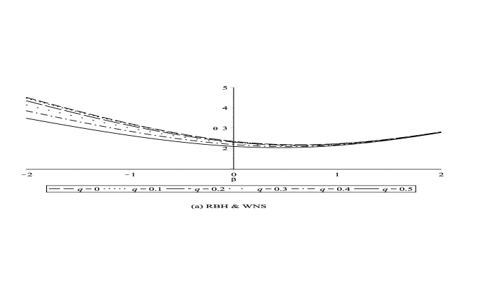
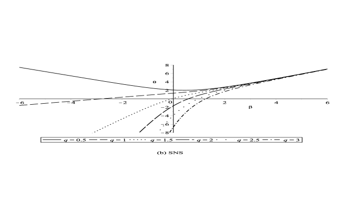
Figure 4:  Diagram of image positions $\theta$ are plotted against source position $\beta$.

where we set $D=0.5$ and $\varepsilon=0.5$ (i.e. $q=m$). Diagram of the image angular position (3.10) is plotted against $\beta$ in figure 4 by using different values of the scalar charge $q$. In figure 4-a we can see that for $q<q_{ph}$, image angular positions have always positive values while will be take negative values for $q\geq q_{ph}$ (see figure 4-b). This means that in case the SNS lens we encounter with image parity transition. It should be noted that the primary (secondary) images $\theta^{+}\,(\theta^{-})$ correspond to the region $\beta>0$ ($\beta<0$), namely they are formed in opposite side of the lens such that $\theta^{-}(\beta)=\theta^{+}(-\beta)$. When we choose $|q|<q_{ph}$ ($|q|>q_{ph}$) the images are formed in the presence (absence) of photon sphere of the Bardeen black hole.
The radius of Einstein rings $\theta_{E}=|\theta_{q}(0)|$ are determined on the vertical axes of the figure 4 with $\beta=0.$ Corresponding equation is given in terms of the parameters $D,$ $q$ and $\varepsilon$ as follows

$$\theta_{E}=\left|1+{\frac{15\pi\varepsilon}{64}}+\left({\frac{20{D}^{2}}{12}}-2D-{\frac{675{\pi}^{2}}{8192}}-{q}^{2}+2\right){\varepsilon}^{2}+\cdots\right|~{}.$$ (3.11)

Radius of Einstein rings are given on vertical axis of figure 4 where the curves are cross with it ($\beta=0$). Radius of rings takes smaller values by increasing scalar charge value for $|q|<q_{ph}$ monotonically but not in case $|q|>q_{ph}.$ In the next section we study magnifications of the determined images.

4 Magnifications

It is well known that the gravitational lensing conserves surface brightness (because of Liouville‘s theorem), but it changes the apparent solid angle of the source. The magnification of an image is defined by the ratio between the solid angles of the image and the source. It is evaluated by

$$\mu=\left|\mu_{t}\,\mu_{r}\right|$$ (4.1)

in which the tangential and radial magnification are given by $\mu_{t}=(\frac{\sin\beta}{\sin\theta})^{-1}$ and $\mu_{r}=(\frac{d\beta}{d\theta})^{-1}$ respectively. Now, we need to obtain expansion series form of the function $\mu$ against $\varepsilon$ as follows

$$\mu=\mu_{0}+\mu_{1}\varepsilon+\mu_{2}\varepsilon^{2}+\cdots$$ (4.2)

where

$$\mu_{0}={\frac{\left({\beta}^{2}+2\right)\sqrt{{\beta}^{2}+4}+\beta\left({\beta}^{2}+4\right)}{2\beta\left({\beta}^{2}+4\right)}},$$ (4.3)

$$\mu_{1}=-{\frac{15\pi}{32\left({\beta}^{2}+4\right)^{3/2}}}$$ (4.4)

and

$$\mu_{2}={\frac{1}{3072\beta\left({\beta}^{2}+4\right)^{3}}}\bigg{[}-\sqrt{{\beta}^{2}+4}\big{(}2048{D}^{2}{\beta}^{4}+61440{D}^{2}{\beta}^{2}+2025{\pi}^{2}{\beta}^{2}+$$

$$18432{\beta}^{2}{q}^{2}-36864\left(D\right){\beta}^{2}+180224{D}^{2}+8100{\pi}^{2}-36864{\beta}^{2}+61440{q}^{2}-122880D$$

$$-122880\big{)}+\beta\left({\beta}^{2}+4\right)\left(16384{D}^{2}+2025{\pi}^{2}+6144{q}^{2}-12288D-12288\right)\bigg{]}~{}.$$ (4.5)

The above coefficients have positive parity $\mu^{+}$ because they are related to primary images $\theta^{+}$. If we want to derive magnification with negative parity $\mu^{-}$ obtained from secondary images $\theta^{-},$ we must replace $\beta$ in the equation (4.2) with $-\beta$ as

$$\mu^{-}(\beta)\equiv\mu^{+}(-\beta)~{}.$$ (4.6)

In cases of gravitational micro-lensing made from distant sources for which positions of primary and secondary images are so close and practically in-distinguishable, then total magnification $\mu_{tot}$ and magnification-weighted centroid $\mu_{cent}$ are two main factors in study of the gravitational lensing. They are defined as

$$\mu_{tot}=|\mu^{+}|+|\mu^{-}|$$ (4.7)

and

$$\mu_{cent}=\frac{\theta^{+}|\mu^{+}|+\theta^{-}|\mu^{-}|}{|\mu^{+}|-|\mu^{-}|}~{}.$$ (4.8)

Using (4.2), (4.3), (4.4), (4.5) and (4.6) one can obtain Taylor series expansion of the equations (4.7) and (4.8) respectively as follows.

$$\mu_{tot}={\frac{{\beta}^{2}+2}{\beta\sqrt{{\beta}^{2}+4}}}+\frac{1}{4}\Big{[}1024\left({\beta}^{2}+4\right)\left({\beta}^{2}+18\right){D}^{2}+6144\left({\beta}^{2}+4\right)\left({q}^{2}-2D\right)$$

$$+2025{\pi}^{2}-12288{\beta}^{2}-49152\Big{]}\varepsilon^{2}+\cdots$$ (4.9)

and

$$\mu_{cent}={\frac{\left({\beta}^{2}+3\right)\beta}{{\beta}^{2}+2}}-{\frac{\beta\left({\beta}^{2}+2\right)^{5}}{1536\left({\beta}^{2}+4\right)^{8}}}\Big{[}-1024\left({\beta}^{2}+4\right)\left({\beta}^{4}+9{\beta}^{2}-2\right){D}^{2}$$

$$+2025{\pi}^{2}+6144{\beta}^{2}\left({\beta}^{2}+4\right)D+6144\left({q}^{2}-2\right)\left({\beta}^{2}+4\right)\Big{]}\varepsilon^{2}+\cdots~{}.$$ (4.10)

Setting $D=0.5,\varepsilon=0.5$ and applying (4.3), (4.4) and (4.5), one can rewrite the magnification (4.2) against $\beta$ and $q$ as that

$$\mu[\theta_{0}(\beta);q]\approx{\frac{{\theta_{0}}^{4}}{{\theta_{0}}^{4}-1}}-{\frac{15\pi{\theta_{0}}^{3}}{64\left({\theta_{0}}^{2}+1\right)^{3}}}+{\frac{1}{6144\left(\theta_{0}^{2}\left({\theta_{0}}^{2}+1\right)^{2}-1\right)^{5}}}\times$$

$$\bigg{[}{\theta_{0}}^{2}\big{(}6144{q}^{2}{\theta_{0}}^{6}+256{\theta_{0}}^{8}+2025{\pi}^{2}{\theta_{0}}^{4}+12288\,{q}^{2}{\theta_{0}}^{4}-13824{\theta_{0}}^{6}+$$

$$6144{\theta_{0}}^{2}{q}^{2}-28160{\theta_{0}}^{4}-13824{\theta_{0}}^{2}+256\big{)}\bigg{]}+\cdots$$ (4.11)

where $\theta_{0}(\beta)$ should be evaluated from the equation (3.7). Setting $D=0.5$, $\varepsilon=0.5$ one can derive total magnification (4.9) and magnification-weighted centroid (4.10) respectively as

$$\mu_{tot}(\beta;q)\approx{\frac{{\beta}^{2}+2}{\beta\sqrt{{\beta}^{2}+4}}}+\frac{1}{16}\Big{[}256\left({\beta}^{2}+4\right)\left({\beta}^{2}+18\right)+6144\left({\beta}^{2}+4\right)\left({q}^{2}-1\right)$$

$$+2025{\pi}^{2}-12288{\beta}^{2}-49152\Big{]}+\cdots$$ (4.12)

and

$$\mu_{cent}(\beta;q)\approx{\frac{\left({\beta}^{2}+3\right)\beta}{{\beta}^{2}+2}}-{\frac{\beta\left({\beta}^{2}+2\right)^{5}}{6144\left({\beta}^{2}+4\right)^{8}}}\Big{[}-256\left({\beta}^{2}+4\right)\left({\beta}^{4}+9{\beta}^{2}-2\right)$$

$$+2025{\pi}^{2}+3072{\beta}^{2}\left({\beta}^{2}+4\right)+6144\left({q}^{2}-2\right)\left({\beta}^{2}+4\right)\Big{]}+\cdots~{}.$$ (4.13)

We have plotted diagrams of the equations (4.11), (4.12) and (4.13) in figures 5, 6 and 7 respectively by regarding different values of the dimensionless charge $q.$ Figures 5 and 6 show that parity of the images obtained in case $|q|>q_{ph}$ is exchanged with respect to ones which obtained in case $|q|<q_{ph}.$ Behavior of magnification-weighted centroid is different (figure 7), namely, it increases monotonically for $|q|<q_{ph}$ but not for $|q|>q_{ph}.$ Also the magnification (and total magnification) of the Einstein rings reduces to infinity for different values of scalar charge $|q|.$ In case $|q|<q_{ph}$ (i.e. black hole and weakly naked singularity), divergence rate increase by increasing values of scalar charge but not in case $|q|>q_{ph}$ (i.e. strongly naked singularity).

5 Concluding remarks

In this paper, we calculated light ray deflection angles with respect to impact parameter for regular Bardeen black hole. This metric contains two characteristics namely charge $g$ and mass $m.$ The photon sphere of black hole appears (disappears) in region of $|q|<q_{ph}$ ($|q|>q_{ph}$) where we defined $q=g/2m$. Applying perturbation series expansion method presented by Keeton et al., we obtained Taylor series expansion of corresponding non-relativistic primary and secondary image positions and also magnifications (total and centroid) as functions of the source position $\beta.$ Physical effects of scalar charge were studied on the parity of images and also the radius of Einstein rings. We have found that for RBH and WNS, the deflection angle decreases, by increasing $|q|$. But there are happened different behaviour for SNS. The non-relativistic image positions become closer to each other for different values of charge parameter by increasing the source angular position $\beta.$ The magnification (and total magnification) of images diverges to infinite value on the location of Einstein rings $\beta=0$ for all values of the scalar charge. Image parity formed from SNS lens are different with respect to image parity made from RBH or WNS lens. Intensity of magnification-weighted centroid in case of SNS is also different with respect to cases RBH or WNS by increasing $\beta$. There is not obtained remarkable difference in the observable quantities as deflection angle, image position and any type of magnification in each cases of RBH and WNS lensing.

References

1.

P. Schneider, J. Ehlers and E. E. Falco, Gravitational lenses, Springer-Verlag, Berlin (1992).

2.

A. O. Petters, H. Levine and J. Wambsganss, Singularity Theory and Gravitational Lensing, Boston-Birkhauser, (2001).

3.

R. Epstein and I. I. Shapiro, Phys. Rev. D 22, 2947 (1980).

4.

M. Sereno, Phys. Rev. D 69, 023002 (2004).

5.

C. R. Keeton and A. O. Petters, Phys. Rev. D 72, 104006 (2005).

6.

M. Sereno and F. De Luca, Phys. Rev. D 74, 123009 (2006).

7.

M. C. Werner and A. O. Petters, Phys. Rev. D 76, 064024 (2007).

8.

S. Frittelli, T. P. Kling, and T. Newman, Phys. Rev. D 61, 064021 (2000).

9.

V. Bozza, Phys. Rev. D 66, 103001 (2002).

10.

V. Bozza, Phys. Rev. D 67, 103006 (2003).

11.

V. Bozza, F. De Luca, G. Scarpetta, and M. Sereno, Phys. Rev. D 72, 083003 (2005).

12.

V. Bozza, F. De Luca, and G. Scarpetta, Phys. Rev. D 74, 063001 (2006).

13.

R. Whisker, Phys. Rev. D 71, 064004 (2005).

14.

E. F. Eiroa, Phys. Rev. D 71, 083010 (2005).

15.

E. F. Eiroa, Phys. Rev. D 73, 043002 (2006).

16.

K. Sarkar and A. Bhadra, Class. Quantum. Grav.23, 6101 (2006), gr-qc/0602087.

17.

Eiroa, E.F. and Sendra. C.M., Class. Quantum Grav. 28, 085008 (2011).

18.

Virbhadra, K. S., and Keeton, C. R., Phys. Rev. D, 77, 124014, (2008).

19.

Virbhadra, K.S., Int. J. Mod. Phys. A, 12, 4831, (1997).

20.

Virbhadra, K.S., Phys. Rev. D, 79, 083004, (2009).

21.

Virbhadra, K.S., and Ellis, G.F.R., Phys. Rev. D, 62, 084003, (2000).

22.

Virbhadra, K.S., and Ellis, G.F.R., Phys. Rev. D, 65, 103004, (2002).

23.

Virbhadra, K.S., Narasimha, D., and Chitre, S.M., Astron. Astrophys., 337, (1998).

24.

Amore, P., and Arceo, S. Phys. Rev. D, 73, 083004, (2006).

25.

Amore, P., Arceo, S., and Fern andez, F. M. Phys. Rev. D, 74, 083004, (2006).

26.

Iyer, S. V., and Petters, A.O., Gen. Relativ. Gravit., 39, 1563, (2007).

27.

Bozza V. Gen, Rel. Grav. 42, 2269 (2010).

28.

Bardeen J, Proc. GR5 (Tiflis, USSR) (1968).

29.

Borde A. Phys. Rev. D50, 3692 (1994).

30.

Borde A. Phys. Rev. D55, 7615 (1997).

31.

Ayon Beato E and Garcia A, Phys. Lett. B493, 149 (2000).

32.

Ansoldi S, gr-qc/0802.0330 (2008).

33.

Pradhan P., gr-qc/1402.2748v2 (2014).

34.

C. M. Claudel, K. S. Virbhadra and G. F. R. Ellis, J. Math. Phys. 42, 818 , (2001).

35.

C. R. Keeton and A. O. Petters, Phys. Rev. D 72, 104006 (2005).

36.

V. Bozza, Phys. Rev. D78, 103005 (2008).

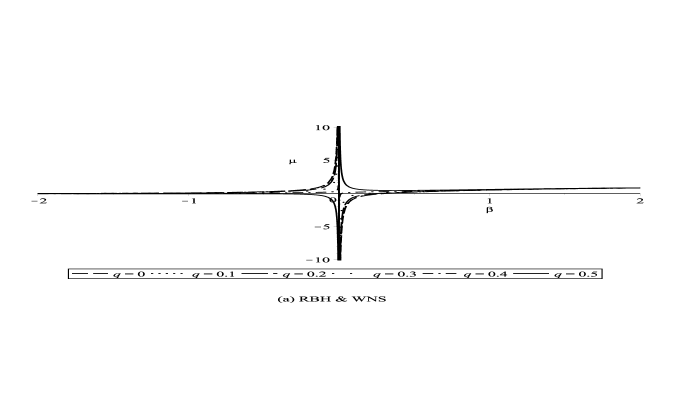
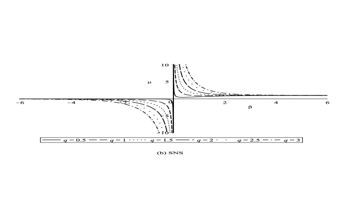
Figure 5:  Diagram of magnification $\mu$ is plotted against source position $\beta$.

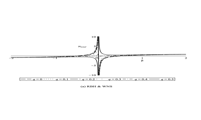
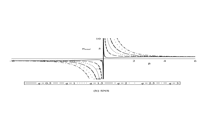
Figure 6:  Diagram of total magnification $\mu_{tot}$ is plotted against source position $\beta$.

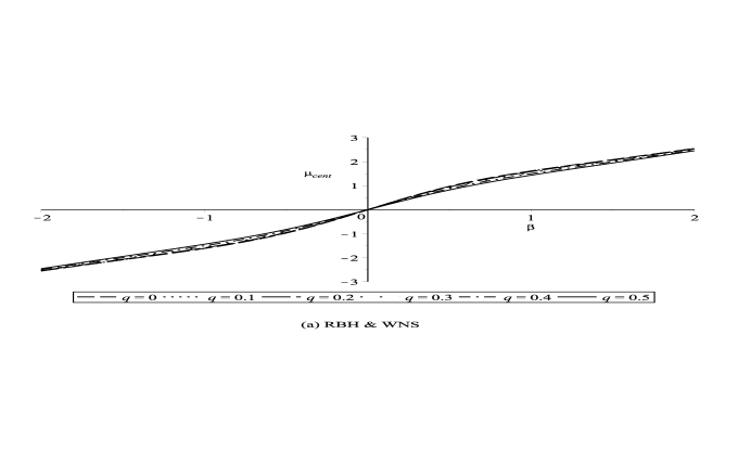
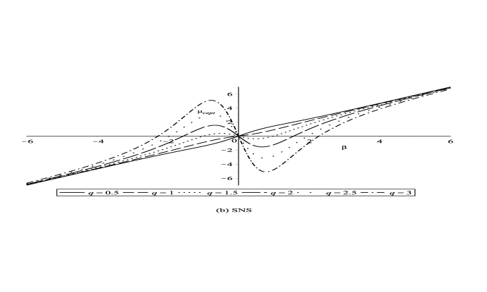
Figure 7:  Diagram of the magnification-weighted centroid $\mu_{cent}$ is plotted against source position $\beta$.