ON THE ROLE OF ROTATION IN THE OUTFLOWS OF THE CRAB PULSAR

Abstract

In order to study constraints imposed on kinematics of the Crab pulsar’s jet we consider motion of particles along co-rotating field lines in the magnetosphere of the Crab pulsar. It is shown that particles following the co-rotating magnetic field lines may attain velocities close to observable values. In particular, we demonstrate that if the magnetic field lines are within the light cylinder, the maximum value of the velocity component parallel to the rotation axis is limited by $0.5c$. This result in the context of the $X$-ray observations performed by Chandra X-ray Observatory seems to be quite indicative and useful to estimate the density of field lines inside the jet. Considering the three-dimensional (3D) field lines crossing the light cylinder, we found that for explaining the force-free regime of outflows the magnetic field lines must asymptotically tend to the Archimedes’ spiral configuration. It is also shown that the 3D case may explain the observed jet velocity for appropriately chosen parameters of magnetic field lines.

PACS numbers: Need to be added!

1 Introduction

In 2000 the Chandra X-ray Observatory has monitored the Crab nebula and pulsar in $X$-rays. The observations led to the discovery of a helium-rich torus, visible as an east-west band crossing the pulsar region and confirmed the existence of plasma jets that previously had only been partially observed by earlier telescopes (see Ref. weis). Temporal monitoring of the motion within the jets showed that along these dynamical features plasma flows at speeds of $\sim 0.4c$ (see Ref. crabrev). At the other hand, it is generally acknowledged that the principal source of energy driving all processes in the nebula is the rapidly spinning pulsar, which may force the nearby material to co-rotate. Rotational character of the plasma motion is clearly seen in the observations and it is quite reasonable and meaningful to investigate the influence of the rotation on the plasma dynamics within the jet of the Crab pulsar (henceforth the jet). The origin of the torus and jet-like features have been numerically studied in a series of papers (see Refs. komis_1,delzanna,komis_2) where the authors have performed relativistic magnetohydrodynamic simulations, explaining the major properties of the pulsar outflow. In this paper we consider dynamics of relativistic outflows analytically, focusing on the role of rotation in the observed pattern.

The corresponding flows may be kinematically quite complex because the motion is both rotational and relativistic. According to the standard model of jets it is supposed that the magnetic field is strong enough to provide the co-rotation of plasmas. In particular, the magnetic field in the magnetosphere of the Crab pulsar varies with distance as follows $B\approx 6.7\times 10^{12}\times\left(R_{\star}/R\right)^{3}$Gauss, where $R_{\star}\approx 10^{6}$cm is the neutron star’s radius and $R$ - the distance from its centre. It is clear that close to the star the magnetic induction is of the order of $\sim 6.7\times 10^{12}$G and nearby the light cylinder (LC) surface $\sim 1.6\times 10^{12}$G. One can straightforwardly check that the ratio of magnetic energy density and relativistic plasma energy density is:

$$\frac{B^{2}}{8\pi\gamma mc^{2}n_{{}_{GJ}}}\approx\frac{1.6\times 10^{17}}{\gamma}\times\left(\frac{R_{\star}}{R}\right)^{3}$$ (1)

where $\gamma$ is the Lorentz factor of plasma particles, $n_{{}_{GJ}}=B/(Pce)$ is the Goldreich-Julian number density and $P\approx 0.0332$s is Crab pulsar’s period of rotation. This ratio exceeds unity by many orders of magnitude in the whole extent of the magnetosphere for physically reasonable values of Lorentz factors. Therefore, under such conditions, the particles follow the co-rotating magnetic field lines and are accelerated by the centrifugal force. In the course of time the linear velocity of rotation increases and it becomes impossible for a particle to remain in the rigid rotation regime, especially nearby the LC zone. On the other hand, the observational evidence of the outflows from the Crab pulsar confirms that the plasma particles do go beyond the LC. It can be concluded that close to this area the field lines has to deviate from the linear configuration, either by twisting in a direction perpendicular to the equatorial plane, or by lagging behind the rotation, or, most probably, by twisting in both directions.

In the present paper we investigate the role of centrifugal force on some dynamical features of the jet-like structure visible in the $X$-ray images of the Crab pulsar.

Since co-rotation of plasmas is ensured by the presence of strong magnetic field the corresponding process is called magnetocentrifugal acceleration. A concrete astrophysical application of the magnetocentrifugal acceleration for the pulsar emission theory was considered in Ref. g96, where the author suggested the centrifugal acceleration of the charged particles as the efficient mechanism leading to the generation of high-energy emission. In Ref. osmr09 a plasma-rich pulsar magnetosphere was studied for Crab-like pulsars to examine the role of centrifugal force in producing the high-energy photons. The similar problem was studied for Active Galactic Nuclei (AGN) in Ref. tev,chemiAA,ra8 where it was found that the co-rotation of plasma particles leads to extremely high energy of relativistic electrons, which, in turn, provides TeV energies for soft photons via the inverse Compton scattering.

In order to mimic the jet situation in a realistic way we consider different geometric configurations for magnetic field lines. As a first example we consider the case when magnetic field lines and the axis of rotation are in one plane (that is, $\phi=const$ for the field lines) and show that charged particles with nonrelativistic initial velocities, independently of a shape of magnetic field line, can attain longitudinal velocities up to $\sim 0.5c$. The second class of curves is related to those considered in Ref. r03, where the dynamics of a single particle moving along the prescribed co-rotating trajectory has been studied. Here we find out that under favorable conditions centrifugally accelerated particles may asymptotically reach the force-free regime of motion. A different approach to magnetocentrifugal acceleration was proposed in Refs. bogoval2,bogoval1, although the results were similar to those obtained in Ref. r03. In general, the mentioned work is a two-dimensional (2D) investigation, which, for being applied to the jet-like structures needs to be generalized to the 3D case.

The structure of the paper is following: in Sec. II we develop an analytical method for studying dynamics of the motion of relativistic particles along the prescribed trajectories. In Sec. III we present our results and we summarize them in the Sec. IV.

2 General formalism

The goal of this paper is to consider dynamics of particles inside the jet. In this context we shall study constraints imposed on the motion by the ‘frozen-in’ condition, which prescribes the particles to move along field lines. For this purpose we generalize the method developed in Ref. r03, where only the flat, 2D, equatorial plane trajectories have been considered. In this paper we develop the more general model, which allows to consider centrigufally driven particles moving along arbitrarily general 3D trajectories.

It is well-kinown that the rotation of the central object, i.e. a rapidly rotating neutron star or Kerr black hole, introduces off-diagonal terms in the spacetime metric, which can be generally written as (Ref. s84):

$$ds^{2}=g_{tt}dt^{2}+2g_{t\phi}dtd\phi+g_{\phi\phi}d\phi^{2}+g_{rr}dr^{2}+g_{\theta\theta}d\theta^{2},$$ (2)

with the metric coefficients independent of $t$ and $\phi$. We use geometrical units $G=c=1$. In the nonrelativistic limit this metric reduces to the Minkowskian metric, written in spherical coordinates. In the presence of gravity it comprises both non-rotating (Schwarzschild) and rotating (Kerr) black hole metrics. For instance, the Kerr metric is written as (Ref. ss):

$$g_{tt}=-\left(1-\frac{2Mr}{\Sigma}\right)$$ (3)

$$g_{t\phi}=-\frac{2aMrsin^{2}\theta}{\Sigma}$$ (4)

$$g_{\phi\phi}=sin^{2}\theta\left(r^{2}+a^{2}+\frac{2Mra^{2}sin^{2}\theta}{\Sigma}\right)$$ (5)

$$g_{rr}=\frac{\Sigma}{\Delta}$$ (6)

$$g_{\theta\theta}=\Sigma$$ (7)

where $a\equiv J/M$, $\Sigma\equiv r^{2}+a^{2}cos^{2}\theta$, $\Delta\equiv r^{2}-2Mr+a^{2}$ and $J$ and $M$ are the angular momentum and the mass of the central object, respectively. When $a=0$ it reduces to the case of nonrotating black hole (Schwarzschild metric) and if further $M/r<<1$ it reduces to Minkowksi metric written in spherical $[r,\theta,\phi]$ coordinates.

In certain cases of practical interest the (2) metric can be reduced to the one with cylindrical symmetry. In particular, if we introduce instead of the $r$ and $\theta$ coordinates the $[\rho,~{}z]$ pair via the obvious relations:

$$\rho\equiv rsin\theta,~{}~{}~{}z\equiv rcos\theta,$$ (8)

then Eq. (2) takes the following form:

$$ds^{2}=g_{tt}dt^{2}+2g_{t\phi}dtd\phi+g_{\phi\phi}d\phi^{2}+g_{\rho\rho}d\rho^{2}+2g_{\rho z}d\rho dz+g_{zz}dz^{2}.$$ (9)

Here we have the following connection between new and old metric tensor components:

$$g_{\rho\rho}=\frac{1}{r^{2}}\left[\rho^{2}g_{rr}+\frac{z^{2}}{r^{2}}g_{\theta\theta}\right],$$ (10)

$$g_{\rho z}=g_{z\rho}=\frac{\rho z}{r^{2}}\left[g_{rr}-\frac{g_{\theta\theta}}{r^{2}}\right],$$ (11)

$$g_{zz}=\frac{1}{r^{2}}\left[z^{2}g_{rr}+\frac{\rho^{2}}{r^{2}}g_{\theta\theta}\right].$$ (12)

In particular, it is easy to see that for the Kerr metric, from (6-7) it follows that:

$$g_{\rho z}=\rho z\Phi,$$ (13)

$$g_{\rho\rho}=\frac{\Sigma}{\Delta}-z^{2}\Phi,$$ (14)

$$g_{zz}=\frac{\Sigma}{\Delta}-\rho^{2}\Phi,$$ (15)

where

$$\Phi\equiv\frac{\Sigma}{r^{4}\Delta}(2Mr-a^{2}).$$ (16)

These equations show that switching to cylindrical coordinates in the case of both Schwarzschild and Kerr black holes would bring second off-diagonal element, $g_{\rho z}$, in the metric. That is why it is convenient to develop the theory of prescribed trajectories based on the (2) metric form.

Apart from the possible rotation of the central massive object, plasma particles may have kinematically complex motion involving rotation in the space-time defined by Eq. (2). As we already mentioned the co-rotation is related with strong magnetic fields, forcing plasma particles to move along the field lines. The idea of the “prescribed trajectories” method (Ref r03) is to imprint the shape of trajectories within the metric itself and to study the dynamics of particles, moving along prescribed “rails” (field-lines). This assumption essentially means that, in the framework of the paper, the magnetic energy density exceeds that of the plasma kinetic energy by many orders of magnitude.

Let us consider, in the rest frame of the central body, the following prescribed field line configuration:

$$\varphi=\varphi(r),~{}~{}\theta=\theta(r).$$ (17)

and let us assume that $\omega$ is the angular rotation rate of the central body. Obviously, the azimuthal coordinate in (2) metric is related with $\varphi$ in the following way:

$$\phi=\varphi(r)+\omega t.$$ (18)

Embedding (17) and (18) within the basic (2) metric it is straightforward to derive the metric tensor for the prescribed trajectories:

$$ds^{2}=G_{00}dt^{2}+2G_{01}dtdr+G_{11}dr^{2},$$ (19)

where

$$G_{\alpha\beta}=\left(\begin{array}[]{ccc}g_{tt}+2\omega g_{t\phi}+\omega^{2}g_{\phi\phi},&\acute{\varphi}\left(g_{t\phi}+\omega g_{\phi\phi}\right)\\ \acute{\varphi}\left(g_{t\phi}+\omega g_{\phi\phi}\right),&g_{rr}+\acute{\varphi}^{2}g_{\phi\phi}+\acute{\theta}^{2}g_{\theta\theta}\\ \end{array}\right),$$ (20)

$$\alpha,\beta=\{0;1\},$$

$$\acute{\varphi}\equiv\frac{d\varphi}{dr},\;\;\;\acute{\theta}\equiv\frac{d\theta}{dr}.$$

The dynamics of the particle moving along the prescribed trajectory can be defined in terms of the Lagrangian:

$$L=\frac{1}{2}G_{\alpha\beta}\frac{dx^{\alpha}}{d\tau}\frac{dx^{\beta}}{d\tau},$$ (21)

and the following equation of motion

$$\frac{\partial L}{\partial x^{\alpha}}=\frac{d}{d\tau}\left(\frac{\partial L}{\partial\dot{x}^{\alpha}}\right),$$ (22)

$$\dot{x}^{\alpha}\equiv\frac{dx^{\alpha}}{d\tau}$$

where

$$x^{0}\equiv t,\;\;\;x^{1}\equiv r.$$

Since $t$ is the cyclic coordinate, the corresponding component of the generalized momentum is the conserved quantity. One can show that Eq. (22) for $\alpha=0$ gives the expression of the particle’s energy:

$$E=-\gamma\left(G_{00}+G_{01}v\right)=const,$$ (23)

where $v\equiv dr/dt$ is the radial velocity and

$$dt/d\tau\equiv u^{t}\equiv\gamma=\left(-G_{00}-2G_{01}v-G_{11}v^{2}\right)^{-1/2}$$ (24)

is the Lorentz factor of the particle in the laboratory frame (LF). Combining Eqs. (23,24) one can write a quadratic algebraic equation:

$$v^{2}\left(G_{01}^{2}+E^{2}G_{11}\right)+\left(G_{00}+E^{2}\right)\left(2vG_{01}+G_{00}\right)=0$$ (25)

with the solution that explicitly defines the radial velocity:

$$v={\frac{\sqrt{G_{00}+E^{2}}}{(G_{01}^{2}+E^{2}G_{11})}}{\left[-G_{01}\sqrt{G_{00}+E^{2}}\pm E\sqrt{G_{01}^{2}-G_{00}G_{11}}\right]},$$ (26)

where different signs are related with different initial conditions.

Hereafter we neglect gravitational effects and restrict ourselves with the study of the special-relativistic case. In other words we study motion of particles along prescribed trajectories in the Minkowskian space-time. In this particular case $g_{rr}=1,~{}g_{\theta\theta}=r^{2}$, and as it is clear from (10-12), $g_{\rho\rho}=g_{zz}=1$ and $g_{\rho z}=0$. This is a considerably simplified case, where the space-time metric can be written in cylindrical coordinates in the following way:

$$ds^{2}=-dt^{2}+\rho^{2}d\phi^{2}+d\rho^{2}+dz^{2}.$$ (27)

writing prescribed trajectory definition also in cylindrical coordinates:

$$\varphi=\varphi(\rho),~{}~{}z=f(\rho),~{}~{}\acute{\varphi}\equiv\frac{d\varphi}{d\rho},~{}~{}\acute{f}\equiv\frac{df}{d\rho}.$$ (28)

we can apply the above analysis to this case. Evidently for the $G_{\alpha\beta}$ metric now we have:

$$G_{\alpha\beta}=\left(\begin{array}[]{ccc}-1+\omega^{2}\rho^{2},&\omega\acute{\varphi}\rho^{2}\\ \omega\acute{\varphi}\rho^{2},&1+\acute{\varphi}^{2}\rho^{2}+\acute{f}^{2}\\ \end{array}\right),$$ (29)

3 Results

In this section we are going to consider one class of physically interesting configurations of prescribed trajectories (field lines). As a first example (subsection 3.1) we examine the field lines, which are in the same plane with the axis of rotation: $\varphi=const$, $z=f(\rho)$ and in the next subsection we consider 3D spirals: $\varphi=\varphi(\rho)$, $z=f(\rho)$, which might be especially interesting for studying force-free regime of frozen-in particle motion dynamics. Although we have no definitive clue whether which of these cases is realized in reality, still we are able to show that under certain conditions these results might explain the particle kinematics inside the jets.

3.1 $\varphi=const$, $z=f(\rho)$

Let us study dynamics of particles for the prescribed trajectories in the rotating frame (RF), described by $\varphi=const$, $z=f(\rho)$. By taking into account Eq. (29), one can rewrite Eq. (26):

$$v=\left[\frac{1-\omega^{2}\rho^{2}}{1+\acute{f}^{2}}\left(1-\frac{1-\omega^{2}\rho^{2}}{E^{2}}\right)\right]^{\frac{1}{2}},$$ (30)

where

$$E=\gamma_{0}\left(1-\omega^{2}\rho_{0}^{2}\right),$$ (31)

and $\gamma_{0}$ and $\rho_{0}$ are particle’s initial Lorentz factor and its initial distance from the rotation axis, respectively.

To express the longitudinal velocity (along the field lines), $\upsilon_{{}_{\parallel}}\equiv dl/dt$, by the radial velocity, we can write $dl/dt=\left(dl/d\rho\right)\left(d\rho/dt\right)$, which after taking into account $d\rho/dt=\upsilon$, $dl/d\rho=\sqrt{1+\acute{f}^{2}}$ and Eq. (30) leads to

$$v_{{}_{\parallel}}=\left[\left(1-\omega^{2}\rho^{2}\right)\left(1-\frac{1-\omega^{2}\rho^{2}}{E^{2}}\right)\right]^{\frac{1}{2}}.$$ (32)

Theoretical analysis shows interesting features of Eq. (32). In particular, it is clear that $v_{{}_{\parallel}}$ does not depend on a particular shape of a field line. Furthermore, it is worth noting that if the field line approaches the light cylinder, then particle’s longitudinal velocity must decrease, completely vanishing on the LC surface. Indeed, from Eq. (32) it is clear that when $\rho\rightarrow R_{lc}$ ($R_{lc}\equiv c/\omega$ is the light cylinder radius), then $v_{{}_{\parallel}}\rightarrow 0$. Such a behaviour is expected, because on the light cylinder surface the linear velocity of rotation exactly equals the speed of light, which logically requires that another component of the velocity has to vanish: $v_{{}_{\parallel}}\rightarrow 0$.

If one considers Eq. (32) in the context of outflows, then it is reasonable to study an asymptotic behaviour of $v(\rho)$, for the region: $\rho<R_{lc}$. According to the observational evidence, it is clear that the jets are characterized by highly collimated flow structures. In order to mimic the real jets let us consider a field line configuration, with the following asymptotic behaviour: $\rho\rightarrow R$, $z\rightarrow\infty$ (here $R\leq R_{lc}$). If this is the case, then the jet is fully located inside the light cylinder surface and particles keep moving along the field lines.

To analyze Eq. (32), one has to note that for $\rho\ll R_{lc}$ and $\rho\approx R_{lc}$ the velocity vanishes, therefore $v_{{}_{\parallel}}$ must have maximum in the interval: $0<\rho<R_{lc}$. For simplicity let us introduce a dimensionless parameter $\alpha\equiv\rho/R_{lc}$, then Eq. (32) reduces to:

$$v_{{}_{\parallel}}(\alpha)=\left[\left(1-\alpha^{2}\right)\left(1-\frac{1-\alpha^{2}}{E^{2}}\right)\right]^{\frac{1}{2}}$$ (33)

Apparently the velocity $v_{{}_{\parallel}}(\alpha)$ attains its maximum value when:

$$\frac{dv_{{}_{\parallel}}(\alpha)}{d\alpha}=0,$$ (34)

which has the following solution:

$$\alpha=\sqrt{1-\frac{E^{2}}{2}},$$ (35)

leading to an expression for $v_{{}_{\parallel}}^{max}$;

$$v_{{}_{\parallel}}^{max}=\frac{E}{2}.$$ (36)

Since we are interested in the role of rotation in the acceleration process, it is reasonable to consider initially a non relativistic particle ($v_{0}\ll 1$) located on the axis of rotation ($\rho_{0}=0$). From Eq. (31), one can show that the maximum possible velocity might be attained for $\alpha=1/\sqrt{2}$ and the corresponding value equals $v_{{}_{\parallel}}^{max}=0.5$.

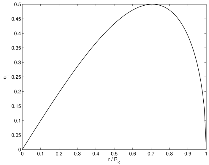
Figure 1: The dependence of the longitudinal velocity on the dimensionless distance. It is assumed that initially particles are nonrelativistic, $E=1$.

On Fig. 1 we show the dependence of the longitudinal velocity on the dimensionless distance. It is clear that at approximately $0.7R_{lc}$ ($R_{lc}/\sqrt{2}$ is the exact analytic value) the velocity reaches its maximum value: $0.5$. This result can be interpreted as follows: if we assume that magnetic field lines have asymptotes (parallel to the axis of rotation) on $R_{lc}/\sqrt{2}$, the longitudinal velocity of the particles will be limited by $0.5$.

One has to note that this velocity is not the jet velocity itself. Therefore, it is interesting to discuss this particular problem in more detail. As we have already specified, charged particles moving along the magnetic field lines with asymptotes along the axis of rotation, “create” a bulk flow - jet. In order to determine the velocity of the whole jet, we should take into account all particles. We introduce a quantity $d(\rho)$ describing the density of asymptotic magnetic field lines. By setting up the normalization condition $\int_{0}^{R_{lc}}d(\rho)d\rho=1$ one can directly calculate the velocity of a jet

$$v_{Jet}=\int_{0}^{R_{lc}}d(\rho)v_{{}_{\parallel}}(\rho)d\rho,$$ (37)

where we have assumed that the particles are uniformly distributed on the field lines. Let us assume that in the asymptotic region the field lines are distributed uniformly as well. Then, for the jet velocity one obtains the value $1/3$, but the observations show that the bulk flow along the Crab jet moves approximately with $0.4$. This means that the magnetic field lines must not be distributed uniformly and density of field lines has to be a continuously increasing function close to the LC surface. For example, one can check that the best fit to observations ($v_{Jet}\sim 0.4$) is provided by the following behaviour of the density of asymptotic field lines: $d\propto\rho^{9/5}$.

3.2 $\varphi=\varphi(\rho)$, $z=f(\rho)$

In Ref. r03 motion of a single particle, sliding along a curved rotating channel (located in the equatorial plane) has been studied. It was shown that under certain conditions, if the particles follow trajectories having a shape of the Archimedes spiral, the flow may become asymptotically free, reaching sufficiently high Lorentz factors at the infinity. It is natural to generalize the approach developed in Ref. r03 for 3D case and check when and how can centrifugally accelerated particles, moving along prescribed 3D trajectories, go beyond the LC.

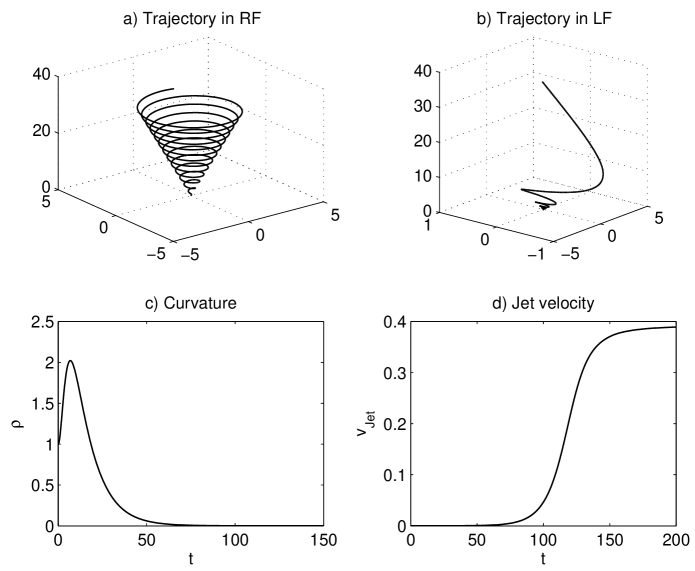
Figure 2: On the top panel we show the particle trajectories in (a) the rotational frame of reference and (b) the laboratory frame of reference respectively. On graphs (c) and (d) the behaviour of the curvature ($\kappa\equiv 1/R_{c}$, where $R_{c}$ is the curvature radius of magnetic field lines) and jet velocity is shown respectively. The set of parameters is: $\acute{\varphi}=-28$, $\acute{f}=11$, $v_{0}=0.01$ and $\rho_{0}=0$.

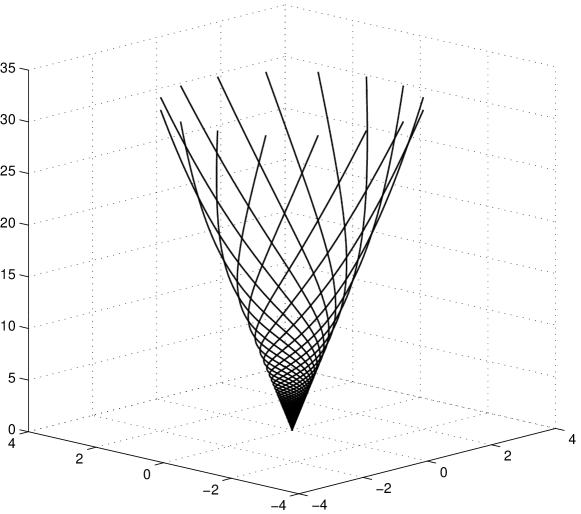
Figure 3: The graph shows the trajectories of particles in the laboratory frame of reference for several field lines. The set of parameters is the same as in the previous graph, except the initial angular shifts of exactly the same field line configurations.

The goal of this subsection is twofold: for this particular choice of the prescribed 3D trajectories we would like to: (a) understand how particles achieve the force-free regime for $\rho\rightarrow\infty$ and (b) intend to explain the jet velocities observed by the Chandra X-ray Observatory. In this context, for proper initial conditions, it is useful to specify from Eq. (26), the asymptotic behavior of the radial velocity:

$$v\rightarrow-\frac{\omega}{\acute{\varphi}}+\frac{1}{\rho^{2}\omega\acute{\varphi}}\left(E^{2}-1+\frac{E\sqrt{\acute{\varphi}^{2}-\omega^{2}\left(1+\acute{f}^{2}\right)}}{\acute{\varphi}}\right),$$ (38)

which makes sense if both conditions $|\acute{\varphi}|\geq|\omega\sqrt{1+\acute{f}^{2}}|$ and $\acute{\varphi}<0$ are simultaneously fulfilled. Then, as we see, the particles will reach infinity with the radial velocity asymptotically tending to $\omega/|\acute{\varphi}|$. The reason why particles can cross the LC, without violating the causality principle of relativity is hidden in Eq. (38). In particular, assuming $\{|\acute{\varphi}|,|\acute{f}|\}<\infty$ it is clear that $\Omega\equiv\omega+v\acute{\varphi}\propto 1/\rho^{2}$, which in turn is nothing but the so called effective angular velocity of rotation (see Ref. r03, Eq. 11). Therefore, the trajectory of the particle in the lab frame must asymptotically become a straight line. The aforementioned behaviour does not mean the acceleration is inefficient and the role of centrifugal effects is insignificant. In particular, as it is clear from the definition of the effective angular velocity, the asymptotic radial velocity (and hence the total velocity) depends on a shape of the spiral, $-\omega/\acute{\varphi}$, which means that the particles reaching extremely high values of Lorentz factors in the force-free regime move along the magnetic field lines with a different parameter, $\acute{\varphi}$. Therefore, to study the overall picture of dynamics one has to take into account different Archimedes spirals allowing different Lorentz factors of particles.

On the other hand, since the force-free motion is characterized by constant velocity, then both, $\acute{\varphi}$ and $\acute{f}$ must asymptotically tend to constant values.

For studying the prescribed trajectories satisfying the mentioned conditions, it is more convenient to write down an expression for the radial acceleration:

$$\ddot{\rho}=\rho\Omega\frac{\omega-{\gamma}^{2}v\left[\acute{\varphi}+\left(1+\acute{f}^{2}\right)\omega v\right]}{\gamma^{2}\left[\left(1+\acute{f}^{2}\right)\left(1-\omega^{2}\rho^{2}\right)+\acute{\varphi}^{2}\rho^{2}\right]}.$$ (39)

As it is evident from this expression, the radial acceleration is proportional to the effective angular velocity, which, as we have already seen, asymptotically vanishes and completely terminates the subsequent acceleration.

It is worth noting that the jet velocity, $v_{Jet}\equiv dz/dt$, is expressed as follows: $v_{Jet}=\omega|{\acute{f}}/{\acute{\varphi}}|$. Apart from that, according to the observations, the jet of the Crab pulsar has the velocity of the order of $0.4$, which means that the two functions describing the field configuration asymptotically must yield the following condition: $|{\acute{f}}/{\acute{\varphi}}|={0.4}/{\omega}$

On Fig. (2) (top panel) we show the trajectories of a particle in (a) the rotational frame of reference and (b) the laboratory frame of reference, respectively. On graphs (c) and (d) the behaviour of the curvature ($\kappa\equiv 1/R_{c}$, where $R_{c}$ is the curvature radius of magnetic field lines) and jet velocity is shown respectively. The set of parameters is: $\acute{\varphi}=-28$, $\acute{f}=11$, $v_{0}=0.01$ and $\rho_{0}=0$. As it is clear from the graphs, if the particle’s trajectory in the RF is presented by the spiral (see a), from the point of view of an observer in the LF the trajectory asymptotically becomes a straight line (see b). With the plot shown on the bottom panel - (c), we show the time dependence of the curvature normalized on the initial value. As it is clear from its behaviour, in due course of time the curvature tends to zero, which means that the trajectory becomes rectilinear and the particle dynamics reaches the force-free regime. In particular, as we see on plot (d), the jet velocity initially increases and asymptotically tends to $0.4$. The aforementioned parameters are chosen so that the numerical results to be in a good agreement with the observations. On Fig. 3 we show the trajectories of particles in the laboratory frame of reference. As it is clear from the figure, the envelope of the trajectories produces the conical surface, that was initially determined by our choice - see plot (a) on Fig. 2. It is worth noting, that this choice was natural because, for the outflow to be in the force-free regime, the only way is to have the 3D spiral form (in the RF) with the properties of the archimedes spiral.

On the other hand, as it has already been shown, such a configuration of magnetic field might be guaranteed by the curvature drift instability, inevitably leading to the creation of a toroidal component of magnetic field (see Ref. odm08). This in turn, changes the structure of field lines, asymptotically acquiring a shape of Archimedes spiral, that finally suspends the consequent amplification of the toroidal magnetic field (see Ref. osm09). It is worth noting that in the framework of a rather different approach the same configuration of magnetic field lines has been derived in (Ref. buckley).

4 Summary

1. For the general gravitational field produced by a rotating object, the method for studying particle dynamics on prescribed, rotating, 2D and 3D trajectories has been developed.

2. We have examined two cases of prescribed trajectories. As a first example, field lines asymptotically becoming parallel to the axis of rotation have been studied. It was shown that if these lines are inside the light cylinder surface, for initially nonrelativistic particles, the maximum attainable velocity along the axis of rotation must be limited by $0.5c$. We have also discussed the compatibility of this result with observations (stating that the velocity of the Crab jet is of the order of $\sim 0.4$c) and we have shown that in order for the theory to be in a good agreement with observations the best fit for the behaviour of density of asymptotic field lines must be given as $\rho^{9/5}$.

3. We also studied a 3D generalization of spiral trajectories, examined in Ref. r03. It has been shown that under certain conditions, particles following the co-rotating field lines, will asymptotically reach the force-free regime of motion if the 3D field-lines are of the shape of Archimedes spiral. We have found that for properly selected parameters one can explain the observed numerical value of the velocity of the jet.

The aim of the paper was to show a role of rotation in the jet-like structure of the Crab pulsar. The study was only focused on the dynamic behaviour of particles, moving along prescribed (in the RF) co-rotating channels.

An important restriction in the present model is the consideration of a single particle approach, whereas it is clear that in a general case dynamics of particles is strongly influenced by collective phenomena. Therefore, it would be interesting to explore the dynamics of magnetocentrifugally accelerated particles in this context.

The formalism developed in Section 2 is valid for both Schwarzschild and Kerr black holes even though in the subsequent analysis we completely neglected the gravitational effects and considered only a special-relativistic case. One of the tasks of further study will be to check how magnetocentrifugal acceleration along prescribed trajectories works in fully relativistic situations and physically realistic astrophysical scenarios.

References

- [1] Weisskopf et al. 2000, ApJL, 536, 81
- [2] Hester J.J., 2008, ARA&A, 46, 127
- [3] Komissarov, S.S. & Lyubarsky, Y.E., 2003, MNRAS, 344, L93
- [4] Del Zanna, L., Amato, E. & Bucciantini, N., 2004, A&A, 421, 1063
- [5] Oliver, P., Komissarov, S.S. & Keppens, R., 2014, MNRAS, 438, 278
- [6] Gangadhara, R. T. 1996, A&A, 314, 853
- [7] Osmanov Z. & Rieger F., 2009, A&A, 502, 15
- [8] Osmanov Z., 2010, New Astronomy, 15, 351
- [9] Osmanov, Z. Rogava, A. & Bodo, G., 2007, A&A, 470, 395O
- [10] Rieger F. M. & Aharonian F. A., 2008, A&A, 479, 5
- [11] Rogava, A. D., Dalakishvili, G. & Osmanov, Z.N., 2003, Gen. Rel. and Grav. 35, 1133
- [12] Bogovalov, S., 2001, A&A, 367, 159
- [13] Bogovalov, S. & Tsinganos, K., 1999, MNRAS, 305, 211
- [14] Straumann, N., General Relativity and Relativistic Astrophysics, Springer, Berlin, 1984,
- [15] Shapiro, S. L., and Teukolsky, S. A., Black Holes, White Dwarfs and Neutron Stars, Wiley, 2004.
- [16] Osmanov, Z., Dalakishvili, G. & Machabeli, G., 2008, MNRAS, 383, 1007
- [17] Osmanov, Z., Shapakidze, D. & Machabeli, G., 2009, A&A, 503, 19
- [18] Buckley, R., 1977, MNRAS, 180, 125