SNSN-323-63

Standard Model updates and new physics analysis with the Unitarity Triangle fit

A. Bevan^a, M. Bona^a,, M. Ciuchini^b, D. Derkach^c, E. Franco^d, V. Lubicz^e, G. Martinelli^d,f, F. Parodi^g, M. Pierini^h, C. Schiavi^g, L. Silvestrini^d, V. Sordiniⁱ, A. Stocchi^j, C. Tarantino^e, and V. Vagnoni^k
UTfit Collaboration

^aQueen Mary University of London

^bINFN, Sezione di Roma Tre

^cUniversity of Oxford

^dINFN, Sezione di Roma

^eINFN, Sezione di Roma Tre, and Università di Roma Tre

^fSISSA-ISAS

^gUniversità di Genova and INFN

^hCalifornia Institute of Technology

ⁱIPNL-IN2P3 Lyon

^jIN2P3-CNRS et Université de Paris-Sud

^kINFN, Sezione di Bologna

We present here the update of the Unitarity Triangle (UT) analysis performed by the UTfit Collaboration within the Standard Model (SM) and beyond. Continuously updated flavour results contribute to improving the precision of several constraints and through the global fit of the CKM parameters and the SM predictions. We also extend the UT analysis to investigate new physics (NP) effects on $\Delta F=2$ processes. Finally, based on the NP constraints, we derive upper bounds on the coefficients of the most general $\Delta F=2$ effective Hamiltonian. These upper bounds can be translated into lower bounds on the scale of NP that contributes to these low-energy effective interactions.

PRESENTED AT

8th International Workshop on the CKM Unitarity Triangle (CKM 2014), Vienna, Austria, September 8-12, 2014

1 Introduction

One of the main tasks of Flavor Physics is an accurate determination of the parameters of the Cabibbo-Kobayashi-Maskawa (CKM) matrix. It represents a crucial test of the SM and, moreover, improving the accuracy on the CKM parameters is at the heart of many searches for NP, where small NP effects are looked for.

2 Unitarity Triangle Analysis in the SM

The Unitarity Triangle (UT) analysis presented here is performed by the UTfit Collaboration following the method described in Refs [1, 2]. From a Bayesian global fit the CKM parameters $\overline{\rho}$ and $\overline{\eta}$ from the Wolfenstein parameterisation are obtained exploiting a plethora of flavour measurements, both theoretical and experimental. The basic constraints are: $\left|V_{ub}/V_{cb}\right|$ from semileptonic $B$ decays, $\Delta m_{d}$ and $\Delta m_{s}$ from $B^{0}_{d,s}$ oscillations, $\varepsilon_{K}$ from $K$ mixing, $\alpha$ from charmless hadronic $B$ decays, $\gamma$ from charm hadronic $B$ decays, and $\sin 2\beta$ from $B^{0}\to J/\psi K^{0}$ decays. The complete set of numerical values used as inputs can be found at the URL http://www.utfit.org . The experimental measurements are mostly taken from Ref. [3], while the non-perturbative QCD parameters come from the most recent lattice QCD averages [4].

Consider the angle $\alpha$ of the CKM triangle: it is extracted from charmless hadronic $B$ decays with the method described in [5]. For this report, we updated the $\alpha$ extraction with the latest input values, in particular using the $B^{0}\to\pi^{0}\pi^{0}$ BR with the new average $(1.15\pm 0.41)\>10^{-6}$, including the latest Belle result [6]. The left plot in Figure 1 shows the effect on the $B^{0}\to\pi^{0}\pi^{0}$ BR values on the $\alpha$ p.d.f., while the middle plot combines the results from the analyses with the other charmless hadronic $B$ decays. This combination gives $\alpha=(92.2\pm 6.2)^{\circ}$.

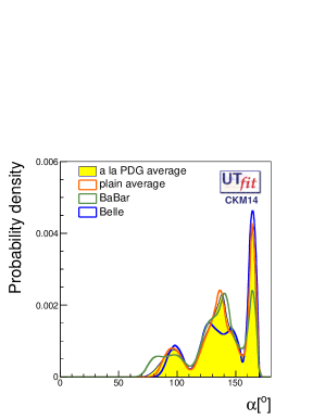
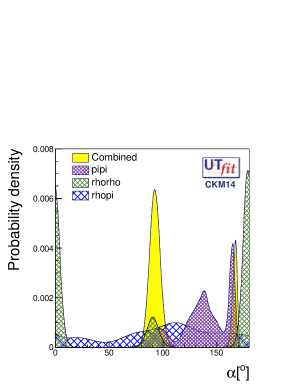
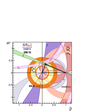
Figure 1: Left: angle $\alpha$ (or $\phi_{2}$) extracted from the $\pi\pi$ isospin analysis with different values of the $B\to\pi^{0}\pi^{0}$ BR. Middle: angle $\alpha$ extracted from the combination of the different charmless $B$ decay systems. Both plots show the one-dimensional p.d.f. for the given variable. Right: $\overline{\rho}-\overline{\eta}$ plane showing the result of the SM fit. The black contours display the 68% and 95% probability regions selected by the given global fit. The 95% probability regions selected by the single constraints are also shown.

Using the above inputs and our Bayesian framework, we perform the global fit to extract the CKM matrix parameters $\overline{\rho}$ and $\overline{\eta}$: we obtain $\overline{\rho}=0.137\pm 0.022$ and $\overline{\eta}=0.349\pm 0.014$. The right plot in Figure 1 shows the result of the SM fit on the $\overline{\rho}$-$\overline{\eta}$ plane.

With the default global fit, it is interesting to extract the UTfit predictions for SM observables. The BR$(B\to\tau\nu)$ is found to be $(0.81\pm 0.07)\cdot 10^{-4}$ in agreement at the level of $\sim 1.4\sigma$ with the experimental measurement of BR$(B\to\tau\nu)=(1.67\pm 0.30)\cdot 10^{-4}$ [3]. The BR$(B_{s}\to\mu\mu)$ is found to be $(3.88\pm 0.15)\cdot 10^{-9}$, while BR$(B^{0}\to\mu\mu)$ is $(1.13\pm 0.07)\cdot 10^{-10}$ to be compared with the recent results by CMS and LHCb Collaborations ($\mbox{\rm BR}(B_{s}\to\mu\mu)=(2.8^{+0.7}_{-0.6})\times 10^{-9}$ and $\mbox{\rm BR}(B^{0}\to\mu\mu)=(3.9^{+1.6}_{-1.4})\cdot 10^{-10}$ [7]).

3 Beyond the SM: Unitarity Triangle Analysis in presence of New Physics

We perform a full analysis of the UT reinterpreting the experimental observables including possible model-independent NP contributions. The possible NP effects considered in the analysis are those entering neutral meson mixing ($\Delta F=2$ transitions) and they can be parameterised in a model-independent way as:

$$C_{B_{q}}\,e^{2i\phi_{B_{q}}} = \frac{\langle B_{q}|H_{\mathrm{eff}}^{\mathrm{full}}|\overline{B}_{q}\rangle}{\langle B_{q}|H_{\mathrm{eff}}^{\mathrm{SM}}|\overline{B}_{q}\rangle}\;\;=\;\;\left(1+\frac{A_{q}^{\mathrm{NP}}}{A_{q}^{\mathrm{SM}}}e^{2i(\phi_{q}^{\mathrm{NP}}-\phi_{q}^{\mathrm{SM}})}\right)$$

where in the SM $C_{B_{d,s}}=1$ and $\phi_{B_{d,s}}=0$, or equivalently $A_{q}^{\mathrm{NP}}=0$ and $\phi_{q}^{\mathrm{NP}}=0$. In addition, $H_{\mathrm{eff}}^{\mathrm{SM}}$ is the SM $\Delta F=2$ effective Hamiltonian, $H_{\mathrm{eff}}^{\mathrm{full}}$ is its extension in a general NP model, and $q=d$ or $s$.

The following experimental inputs are added to the fit to extract information on the $B_{s}$ system: the semileptonic asymmetry in $B_{s}$ decays, the di-muon charge asymmetry, the $B_{s}$ lifetime from flavour-specific final states, and CP-violating phase and the decay-width difference for $B_{s}$ mesons from the time-dependent angular analyses of $B_{s}\to J/\psi\phi$ decays.

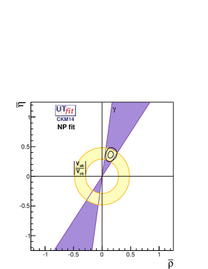
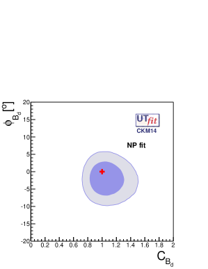
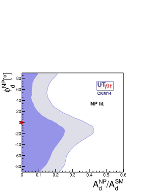
Figure 2: Right: $\overline{\rho}-\overline{\eta}$ plane showing the result of the NP fit. The black contours display the 68% and 95% probability regions selected by the given global fit. The 95% probability regions selected are also shown for those constraints not affected by NP in $\Delta F=2$ transitions. (Middle-right) NP parameters in the $B_{d}$ system. $68\%$ (dark) and $95\%$ (light) probability regions in the $\phi_{B_{d}}$ – $C_{B_{d}}$ (middle), $\phi_{d}^{\mathrm{NP}}$ – $\frac{A_{d}^{\mathrm{NP}}}{A_{d}^{\mathrm{SM}}}$ (right) planes in the NP fit. The red cross represents the SM expectation.

From the full NP analysis, the global fit selects a region of the $(\overline{\rho},\overline{\eta})$ plane (left plot in Figure 2, with $\overline{\rho}=0.154\pm 0.040$ and $\overline{\eta}=0.367\pm 0.048$) which is consistent with the results of the SM analysis. The NP parameters in the $B_{d}$ and $B_{s}$ systems are also extracted from the fit and found in agreement with the SM expectations: $C_{B_{d}}=0.81\pm 0.12$, $\phi_{B_{d}}=(-3.4\pm 3.6)^{\circ}$, $C_{B_{s}}=0.87\pm 0.09$ and $\phi_{B_{s}}=(-7\pm 5)^{\circ}$. The two right plots in Figure 2 show the values still available for the NP parameters in the $B_{d}$ system. Currently, the ratio of NP/SM amplitudes needs to be less than $25\%$ at $68\%$ probability ($42\%$ at $95\%$ prob.) in $B_{d}$ mixing and less than $17\%$ at $68\%$ prob. ($25\%$ at $95\%$) in $B_{s}$ mixing.

We now consider the most general effective Hamiltonian for $\Delta F=2$ processes ($\mathcal{H}_{\mathrm{eff}}^{\Delta F=2}$) in order to translate the current constraints into allowed ranges for the Wilson coefficients of $\mathcal{H}_{\mathrm{eff}}^{\Delta F=2}$. The full procedure and analysis details are given in [8]. These coefficients have the general form

$$C_{i}(\Lambda)=\frac{F_{i}L_{i}}{\Lambda^{2}}\,$$ (1)

where $F_{i}$ is a function of the (complex) NP flavour couplings, $L_{i}$ is a loop factor that is present in models with no tree-level Flavour Changing Neutral Currents (FCNC), and $\Lambda$ is the scale of NP. For a generic strongly-interacting theory with arbitrary flavour structure, one expects $F_{i}\sim L_{i}\sim 1$ so that the allowed range for each of the $C_{i}(\Lambda)$ can be immediately translated into a lower bound on $\Lambda$.

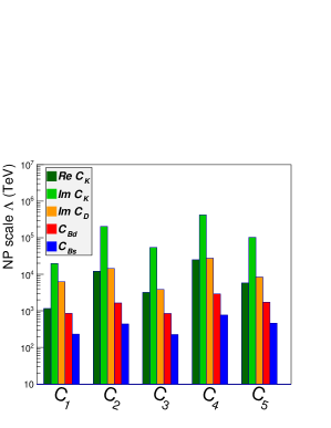
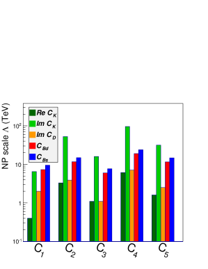
Figure 3: Summary of the $95\%$ probability lower bound on the NP scale $\Lambda$ for strongly-interacting NP in the general NP scenario (left) and in the NMFV scenario (right). Results from all the neutral meson systems are shown.

The left plot in Figure 3 shows the results for the lower bounds on $\Lambda$ coming from all the $C_{i}$’s for all the sectors in the case of the general NP scenario, with arbitrary NP flavour structures ($|F_{i}|\sim 1$) with arbitrary phase and $L_{i}=1$ corresponding to strongly-interacting and/or tree-level NP. To obtain the lower bound on $\Lambda$ for loop-mediated contributions, one simply multiplies the bounds we quote in the following by $\alpha_{s}(\Lambda)\sim 0.1$ or by $\alpha_{W}\sim 0.03$. The right plot in Figure 3 shows the lower bounds on $\Lambda$ in a Next-to-Minimal-Flavour-Violation (NMFV) scenario where the flavour structure is SM-like but with arbitrary phase relative to the SM.

We conclude that any model with strongly interacting NP and/or tree-level contributions is beyond the reach of direct searches at the LHC, while in the case of weak couplings the lower bounds on the NP scale are at the limit of the LHC reach. The flavour sector provides the possibility of indirect searches that remain a fundamental tool to constrain (or detect) NP at scales higher that the LHC can provide.

References

- [1] M. Ciuchini, G. D’Agostini, E. Franco, V. Lubicz, G. Martinelli, et al., “2000 CKM triangle analysis: A Critical review with updated experimental inputs and theoretical parameters,” JHEP, vol. 0107, p. 013, 2001.
- [2] M. Bona et al., “The 2004 UTfit collaboration report on the status of the unitarity triangle in the standard model,” JHEP, vol. 0507, p. 028, 2005.
- [3] Y. Amhis et al., “Averages of B-Hadron, C-Hadron, and tau-lepton properties as of early 2012,” 2012.
- [4] S. Aoki, Y. Aoki, C. Bernard, T. Blum, G. Colangelo, et al., “Review of lattice results concerning low-energy particle physics,” Eur.Phys.J., vol. C74, no. 9, p. 2890, 2014.
- [5] M. Bona et al., “Improved Determination of the CKM Angle alpha from B to pi pi decays,” Phys.Rev., vol. D76, p. 014015, 2007.
- [6] The Belle Collaboration, “New Result on with Full data,” 2014. , presented at ICHEP 2014.
- [7] V. Khachatryan et al., “Observation of the rare decay from the combined analysis of CMS and LHCb data,” 2014.
- [8] M. Bona et al., “Model-independent constraints on operators and the scale of new physics,” JHEP, vol. 0803, p. 049, 2008.