Efficient SimRank Computation via Linearization

SimRank, proposed by Jeh and Widom, provides a good similarity measure that has been successfully used in numerous applications. While there are many algorithms proposed for computing SimRank, their computational costs are very high.

In this paper, we propose a new computational technique, “SimRank linearization,” for computing SimRank, which converts the SimRank problem to a linear equation problem. By using this technique, we can solve many SimRank problems, such as single-pair compuation, single-source computation, all-pairs computation, top $k$ searching, and similarity join problems, efficiently.

1 Introduction

1.1 Background and motivation

Very large-scale networks are ubiquitous in today’s world, and designing scalable algorithms for such huge network has become a pertinent problem in all aspects of compute science. The primary problem is the vast size of modern graph datasets. For example, the World Wide Web currently consists of over one trillion links and is expected to exceed tens of trillions in the near future, and Facebook embraces over 800 million active users, with hundreds of billions of friend links.

Large graphs arise in numerous applications where both the basic entities and the relationships between these entities are given. A graph stores the objects of the data on its vertices, and represents the relations among these objects by its edges. For example, the vertices and edges of the World Wide Web graph correspond to the webpages and hyperlinks, respectively. Another typical graph is a social network, whose vertices and edges correspond to personal information and friendship relations, respectively.

With the rapidly increasing amount of graph data, the similarity search problem, which identifies similar vertices in a graph, has become an important problem with many applications, including web analysis [Jeh and Widom (2002), Liben-Nowell and Kleinberg (2007)], graph clustering [Yin et al. (2006), Zhou et al. (2009)], spam detection [Gyöngyi et al. (2004)], computational advertisement [Antonellis et al. (2008)], recommender systems [Abbassi and Mirrokni (2007), Yu et al. (2010)], and natural language processing [Scheible (2010)].

Several similarity measures have been proposed. For example, bibliographic coupling [Kessler (1963)], co-citation [Small (1973)], P-Rank [Zhao et al. (2009)], PageSim [Lin et al. (2006)], Extended Nearest Neighborhood Structure [Lin et al. (2007)], MatchSim [Lin et al. (2012)], and so on. In this paper, we consider SimRank, a link-based similarity measure proposed by Jeh and Widom [Jeh and Widom (2002)] for searching web pages. SimRank supposes that “two similar pages are linked from many similar pages.” This intuitive concept is formulated by the following recursive definition: For a graph $G=(V,E)$, the SimRank score $s(i,j)$ of a pair of vertices $(i,j)\in V\times V$ is recursively defined by

$$s(i,j):=\begin{cases}1,&i=j,\\ \displaystyle\frac{c}{|{\delta}(i)||{\delta}(j)|}\sum_{i^{\prime}\in{\delta}(i),j\in{\delta}(j)}s(i^{\prime},j^{\prime}),&i\neq j,\end{cases}$$ (1.1)

where ${\delta}(i)=\{j\in V:(j,i)\in E\}$ is the set of in-neighbors of $i$, and $c\in(0,1)$ is a decay factor usually set to $c=0.8$ [Jeh and Widom (2002)] or $c=0.6$ [Lizorkin et al. (2010)]. See Figure 1.1 for an example of the SimRank on a small graph.

SimRank can be regarded as a label propagation [Zhu and Ghahramani (2002)] on the squared graph. Let us consider a squared graph $G^{2}=(V^{(2)},E^{(2)})$ whose vertices are the pair of vertices $V^{(2)}=V\times V$ and edges are defined by

$$E^{(2)}=\{((i,j),(i^{\prime},j^{\prime})):(i,i^{\prime}),(j,j^{\prime})\in E\}.$$ (1.2)

Then the SimRank is a label propagation method with trivial relations $s(i,i)=1$ (i.e., $i$ is similar to $i$) for all $i\in V$ on $G^{(2)}$.

SimRank also has a “random-walk” interpretation. Let us consider two random walks that start from vertices $i$ and $j$, respectively, and follow the in-links. Let $i^{(t)}$ and $j^{(t)}$ be the $t$-th position of each random walk, respectively. The first meeting time $\tau_{i,j}$ is defined by

$$\tau_{ij}=\min\{t:i^{(t)}=j^{(t)}\}.$$ (1.3)

Then SimRank score is obtained by

$$s(i,j)=\mathbb{E}[c^{\tau_{i,j}}].$$ (1.4)

$i$	$j$	$s(i,j)$
1	2	0.260
1	3	0.142
1	4	0.120
1	5	0.162
1	6	0.069
1	7	0.219
2	3	0.121

$i$	$j$	$s(i,j)$
2	4	0.141
2	5	0.132
2	6	0.069
2	7	0.226
3	4	0.128
3	5	0.230
3	6	0.236

$i$	$j$	$s(i,j)$
3	7	0.101
4	5	0.107
4	6	0.080
4	7	0.125
5	6	0.271
5	7	0.110
6	7	0.061

Figure 1.1: Example of the SimRank. $c=0.6$.

SimRank and its related measures (e.g., SimRank++ [Antonellis et al. (2008)], S-SimRank [Cai et al. (2008)], P-Rank [Zhao et al. (2009)], and SimRank^∗ [Yu et al. (2013)]) give high-quality scores in activities such as natural language processing [Scheible (2010)], computational advertisement [Antonellis et al. (2008)], collaborative filtering [Yu et al. (2010)], and web analysis [Jeh and Widom (2002)]. As implied in its definition, SimRank exploits the information in multihop neighborhoods. In contrast, most other similarity measures utilize only the one-step neighborhoods. Consequently, SimRank is more effective than other similarity measures in real applications.

Although SimRank is naturally defined and gives high-quality similarity measure, it is not so widely used in practice, due to high computational cost. While there are several algorithms proposed so far to compute SimRank scores, unfortunately, their computation costs (in both time and space) are very expensive. The difficulty of computing SimRank may be viewed as follows: to compute a SimRank score $s(u,v)$ for two vertices $u,v$, since (1.1) is defined recursively, we have to compute SimRank scores for all $O(n^{2})$ pairs of vertices. Therefore it requires $O(n^{2})$ space and $O(n^{2})$ time, where $n$ is the number of vertices. In order to reduce this computation cost, several approaches have been proposed. We review these approaches in the following subsection.

1.2 Related Work

In order to reduce this computation cost, several approaches have been proposed [Fogaras and Rácz (2005), He et al. (2010), Li et al. (2010a), Li et al. (2010b), Lizorkin et al. (2010), Yu et al. (2010), Yu et al. (2013), Yu et al. (2012)]. Here, we briefly survey some existing computational techniques for SimRank. We summarize the existing results in Table 1.4. Let us point out that there are three fundamental problems for SimRank: (1) single-pair SimRank to compute $s(u,v)$ for given two vertices $u$ and $v$, (2) single-source SimRank to compute $s(u,v)$ for a given vertex $u$ and all other vertices $v$, and (3) all-pairs SimRank to compute $s(u,v)$ for all pair of vertices $u$ and $v$.

In the original paper by Jeh and Widom [Jeh and Widom (2002)], all-pairs SimRank scores are computed by recursively evaluating the equation (1.1) for all $u,v\in V$. This “naive” computation yields an $O(Td^{2}n^{2})$ time algorithm, where $T$ denotes the number of iterations and $d$ denotes the average degree of a given network. Lizorkin et al. [Lizorkin et al. (2010)] proposed a “partial sum” technique, which memorizes partial calculations of Jeh and Widom’s algorithm to reduce the time complexity of their algorithm. This leads to an $O(T\min\{nm,n^{3}/\log n\})$ algorithm. Yu et al. [Yu et al. (2012)] applied the fast matrix multiplication [Strassen (1969), Williams (2012)] and then obtained an $O(T\min\{nm,n^{\omega}\})$ algorithm to compute all pairs SimRank scores, where $\omega<2.373$ is the exponent of matrix multiplication. Note that the space complexity of these algorithms is $O(n^{2})$, since they have to maintain all SimRank scores for each pair of vertices to evaluate the equation (1.1). This results is, so far, the state-of-the-art algorithm to compute SimRank scores for all pairs of vertices.

There are some algorithms based on a random-walk interpretation (1.4). Fogaras and Rácz [Fogaras and Rácz (2005)] evaluate the right-hand side by Monte-Carlo simulation with a fingerprint tree data structure, and they obtained a faster algorithm to compute single pair SimRank score for given two vertices $i,j$. Li et al. [Li et al. (2010b)] also proposed an algorithm based on the random-walk iterpretation; however their algorithm is an iterative algorithm to compute the first meeting time and computes all-pairs SimRank deterministically.

Some papers proposed spectral decomposition based algorithms (e.g., [Fujiwara et al. (2013), He et al. (2010), Li et al. (2010a), Yu et al. (2010), Yu et al. (2013)]), but there is a mistake in the formulation of SimRank. On the other hand, their algorithms may output reasonable results. We shall mention more details about these algorithms in Remark 2.2.

1.3 Contribution

In this paper, we propose a novel computational technique for SimRank, called SimRank linearlization. This technique allows us to solve many kinds of SimRank problems such as the following:

Single-pair SimRank

We are given two vertices $i,j\in V$, compute SimRank score $s(i,j)$.

Single-source SimRank

We are given a vertex $i\in V$, compute SimRank scores $s(i,j)$ for all $j\in V$.

All-pairs SimRank

Compute SimRank scores $s(i,j)$ for all $i,j\in V$.

Top $k$ SimRank search

We are given a vertex $i\in V$, return $k$ vertices $j$ with $k$ highest SimRank scores.

SimRank join

We are given a threshold $\delta$, return all pairs $(i,j)$ such that $s(i,j)\geq\delta$.

For all problems, the proposed algorithm outperforms the existing methods.

1.4 Organization

The paper consists of four parts. In Section 2, we introduce the SimRank linearization technique and show that how to use the linearization to solve single-pair, single-source, and all-pairs problem. In Section 3, we describe how to solve top $k$ SimRank search problem. In Section 4, we describe how to solve SimRank join problem. Each section contains computational experiments.

Complexity of SimRank algorithms. $n$ denotes the number of vertices, $m$ denotes the number of edges, $d$ denotes the average degree, $T$ denotes the number of iterations, $R$ is the number of Monte-Carlo samples, and $r$ denotes the rank for low-rank approximation. Note that $*$-marked method is based on an incorect formula: see Remark 2.2. Algorithm Type Time Space Technique Proposed (Section 3.5) Single-pair $O(Tm)$ $O(m)$ Linearization Proposed (Section 3.5) Single-source $O(T^{2}m)$ $O(m)$ Linearization Proposed (Section 3.5) All-pairs $O(T^{2}nm)$ $O(m)$ Linearization Proposed (Section 3.5) Top-$k$ search $\ll O(TR)$ $O(m)$ Linearization & Monte Carlo Proposed (Section 3.5) Join $\approx O(\text{output})$ $O(m+\text{output})$ Linearization & Gauss-Southwell [Li et al. (2010b)] Single-pair $O(Td^{2}n^{2})$ $O(n^{2})$ Random surfer pair (Iterative) [Fogaras and Rácz (2005)] Single-pair $O(TR)$ $O(m+nR)$ Random surfer pair (Monte Carlo) [Jeh and Widom (2002)] All-pairs $O(Tn^{2}d^{2})$ $O(n^{2})$ Naive [Lizorkin et al. (2010)] All-pairs $O(T\min\{nm,n^{3}/\log n\})$ $O(n^{2})$ Partial sum [Yu et al. (2012)] All-pairs $O(\min\{nm,n^{\omega}\})$ $O(n^{2})$ Fast matrix multiplication [Li et al. (2009)] All-pairs $O(^{4/3})$ $O(n^{4/3})$ Block partition [Li et al. (2010a)] All-pairs $O(r^{4}n^{2})$ $O(n^{2})$ Singular value decomposition^∗ [Fujiwara et al. (2013)] All-pairs $O(r^{4}n)$ $O(r^{2}n^{2})$ Singular value decomposition^∗ [Yu et al. (2010)] All-pairs $O(n^{3})$ $O(n^{2})$ Eigenvalue decomposition^∗

List of symbols symbol description $G$ directed unweighted graph, $G=(V,E)$ $V$ set of vertices $E$ set of edges $n$ number of vertices, $n=|V|$ $m$ number of edges, $m=|E|$ $i,j$ vertex $e$ edge $\delta(i)$ in-neighbors of of $i$, $\delta(i)=\{j\in V:(j,i)\in E\}$ $P$ transition matrix, $P_{ij}=1/|\delta(j)|$ for $(i,j)\in E$ $s(i,j)$ SimRank of $i$ and $j$ $S$ SimRank matrix, $S_{ij}=s(i,j)$ $D$ diagonal correction matrix, $S=cP^{\top}SP+D$

2 Linearized SimRank

2.1 Concept of linearized SimRank

Let us first observe the difficulty in computing SimRank. Let $G=(V,E)$ be a directed graph, and let $P=(P_{ij})$ be a transition matrix of transpose graph $G^{\top}$ defined by

$$P_{ij}:=\begin{cases}1/|{\delta}(j)|,&(i,j)\in E,\\ 0,&(i,j)\not\in E,\end{cases}$$

where ${\delta}(i)=\{j\in V:(j,i)\in E\}$ denotes the in-neighbors of $i\in V$. Let $S=(s(i,j))$ be the SimRank matrix, whose $(i,j)$ entry is the SimRank score of $i$ and $j$. Then the SimRank equation (1.1) is represented [Yu et al. (2012)] by:

$$S=(cP^{\top}SP)\lor I,$$ (2.1)

where $I$ is the identity matrix, and $\lor$ denotes the element-wise maximum, i.e., $(i,j)$ entry of the matrix $A\lor B$ is given by $\max\{A_{ij},B_{ij}\}$.

In our view, the difficulty in computing SimRank via equation (2.1) comes from the element-wise maximum, which is a non-linear operation. To avoid the element-wise maximum, we introduce a new formulation of SimRank as follows. By observing (2.1), since $S$ and $cP^{\top}SP$ only differ in their diagonal elements, there exists a diagonal matrix $D$ such that

$$S=cP^{\top}SP+D.$$ (2.2)

We call such a matrix $D$ the diagonal correction matrix. The main idea of our approach here is to split a SimRank problem into the following two subproblems:

1. Estimate diagonal correction matrix $D$.

2. Solve the SimRank problem using $D$ and the linear recurrence equation (2.2).

For efficient computation, we must estimate $D$ without computing the whole part of $S$.

To simplify the discussion, we introduce the notion of linearized SimRank. Let $\Theta$ be an $n\times n$ matrix. A linearized SimRank $S^{L}(\Theta)$ is a matrix that satisfies the following linear recurrence equation:

$$S^{L}(\Theta)=cP^{\top}S^{L}(\Theta)P+\Theta.$$ (2.3)

Below, we provide an example that illustrates what linearized SimRank is.

Example 2.1 (Star graph of order $4$).

Let $G$ be a star graph of order $4$ (i.e., $G$ has one vertex of degree three and three vertices of degree one). The transition matrix (of the transposed graph) is

$$P=\begin{bmatrix}0&1&1&1\\ 1/3&0&0&0\\ 1/3&0&0&0\\ 1/3&0&0&0\\ \end{bmatrix},$$

and SimRank for $c=0.8$ is

$$S=\begin{bmatrix}1&0&0&0\\ 0&1&4/5&4/5\\ 0&4/5&1&4/5\\ 0&4/5&4/5&1\\ \end{bmatrix}.$$

Thus, the diagonal correction matrix $D$ is obtained by

$$D=S-cP^{\top}SP=\mathrm{diag}(23/75,1/5,1/5,1/5),$$

Remark 2.2.

Some papers have used the following formula for SimRank (e.g., equation (2) in [Fujiwara et al. (2013)], equation (2) in [He et al. (2010)], equation (2) in [Li et al. (2010a)], and equation (3) in [Yu et al. (2013)]):

$$S=cP^{\top}SP+(1-c)I.$$ (2.4)

However, this formula does not hold; (2.4) requires diagonal correction matrix $D$ to have the same diagonal entries, but Example 2.1 is a counterexample. In fact, matrix $S$ defined by (2.4) is a linearized SimRank $S^{L}(\Theta)$ for a matrix $\Theta=(1-c)I$.

We provide some basic properties of linearized SimRank in Appendix.

2.2 Solving SimRank problems via linearization

In this section, we present our proposed algorithms for SimRank by assuming that the diagonal correction matrix $D$ has already been obtained. All algorithms are based on the same fundamental idea; i.e., in (2.2), by recursively substituting the left hand side into the right hand side, we obtain the following series expansion:

$$S=D+cP^{\top}DP+c^{2}P^{\top 2}DP^{2}+\cdots.$$ (2.5)

Our algorithms compute SimRank by evaluating the first $T$ terms of the above series. The time complexity of the algorithms are $O(Tm)$ for the single-pair problem, $O(T^{2}m)$ for the single-source problem, and $O(T^{2}nm)$ for the all-pairs problem. For all problems, the space complexity is $O(m)$.

2.2.1 Single-pair SimRank

Let $e_{i}$ be the $i$-th unit vector ($i=1,\ldots,n$); then SimRank score $s(i,j)$ is obtained via the $(i,j)$ component of SimRank matrix $S$, i.e., $s(i,j)=e_{i}^{\top}Se_{j}$. Thus, by applying $e_{i}^{\top}$ and $e_{j}$ to both sides of (2.5), we obtain

$$e_{i}^{\top}Se_{j} =e_{i}^{\top}De_{j}+c(Pe_{i})^{\top}DPe_{j}$$

$$+c^{2}(P^{2}e_{i})^{\top}DP^{2}e_{j}+\cdots.$$ (2.6)

Our single-pair algorithm (Algorithm 1) evaluates the right-hand side of (2.2.1) by maintaining $P^{t}e_{i}$ and $P^{t}e_{j}$. The time complexity is $O(Tm)$ since the algorithm performs $O(T)$ matrix vector products for $P^{t}e_{i}$ and $P^{t}e_{j}$ ($t=1,\ldots,T-1$).

Algorithm 1 Single-pair SimRank

1:procedure SinglePairSimRank(i,j)

2:     $\alpha\leftarrow 0$, $x\leftarrow e_{i}$, $y\leftarrow e_{j}$

3:     for $t=0,1,\ldots,T-1$ do

4:         $\alpha\leftarrow\alpha+c^{t}x^{\top}Dy$, $x\leftarrow Px$, $y\leftarrow Py$

5:     end for

6:     Report $S_{ij}=\alpha$

7:end procedure

2.2.2 Single-source SimRank

For the single-source problem, to obtain $s(i,j)$ for all $j\in V$, we need only compute vector $Se_{i}$, because its $j$-th component is $s(i,j)$. By applying $e_{i}$ to (2.5), we obtain

$$Se_{i}=De_{i}+cP^{\top}DPe_{i}+c^{2}P^{\top 2}DP^{2}e_{i}+\cdots.$$ (2.7)

Our single-source algorithm (Algorithm 2) evaluates the right hand side of (2.7) by maintaining $P^{t}e_{i}$ and $P^{t}e_{j}$. The time complexity is $O(T^{2}m)$ since it performs $O(T^{2})$ matrix vector products for $P^{\top t}DP^{t}e_{i}$ ($t=1,\ldots,T-1$).

Algorithm 2 Single-source SimRank

1:procedure SingleSourceSimRank(i)

2:     $\gamma\leftarrow\mathbf{0}$, $x\leftarrow e_{i}$

3:     for $t=0,1,\ldots,T-1$ do

4:         $\gamma\leftarrow\gamma+c^{t}P^{\top t}Dx$, $x\leftarrow Px$

5:     end for

6:     Report $S_{ij}=\gamma_{j}$ for $j=1,\ldots,n$

7:end procedure

Note that, if we can use an additional $O(Tn)$ space, the single-source problem can be solved in $O(Tm)$ time. We first compute $u_{t}=DP^{t}e_{i}$ for all $t=1,\ldots,T$, and store them; this requires $O(Tm)$ time and $O(Tn)$ additional space. Then, we have

$$Se_{i}=u_{0}+cP^{\top}(u_{1}+\cdots(cP^{\top}(u_{t-1}+cP^{\top}u_{T}))\cdots),$$ (2.8)

which can be computed in $O(Tm)$ time. We do not use this technique in our experiment because we assume that the network is very large and hence $O(Tn)$ is expensive.

2.2.3 All-pairs SimRank

Computing all-pairs SimRank is an expensive task for a large network, because it requires $O(n^{2})$ time since the number of pairs is $n^{2}$. To compute all-pairs SimRank, it is best to avoid using $O(n^{2})$ space.

Our all-pairs SimRank algorithm applies the single-source SimRank algorithm (Algorithm 2) for all initial vertices, as shown in Algorithm 3. The complexity is $O(T^{2}nm)$ time and requires only $O(m)$ space. Since the best-known all-pairs SimRank algorithm [Lizorkin et al. (2010)] requires $O(Tnm)$ time and $O(n^{2})$ space, our algorithm significantly improves the space complexity and has almost the same time complexity (since the cost of factor $T$ is much smaller than $n$ or $m$).

It is worth noting that this algorithm is distributed computing friendly. If we have $M$ machines, we assign initial vertices to each machine and independently compute the single-source SimRank. Then the computational time is reduced to $O(T^{2}nm/M)$. This shows the scalability of our all-pairs algorithm.

Algorithm 3 All-pairs SimRank

1:procedure AllPairsSimRank

2:     for $i=1,\ldots,n$ do

3:         Compute SingleSourceSimRank($i$)

4:     end for

5:end procedure

2.3 Diagonal correction matrix estimation

We first observe that the diagonal correction matrix is uniquely determined from the diagonal condition.

Proposition 2.3.

A diagonal matrix $D$ is the diagonal correction matrix, i.e., $S^{L}(D)=S$ if and only if $D$ satisfies

$$S^{L}(D)_{kk}=1,\quad(k=1,\ldots,n),$$ (2.9)

where $S^{L}(D)_{kk}$ denotes $(k,k)$ entry of the linearized SimRank matrix $S^{L}(D)$.

Proof 2.4.

See Appendix.

This proposition shows that the diagonal correction matrix can be estimated by solving equation (2.9). Furthermore, we observe that, since $S^{L}$ is a linear operator, (2.9) is a linear equation with $n$ real variables $D_{11},\ldots,D_{nn}$ where $D=\mathrm{diag}(D_{11},\ldots,D_{nn})$. Therefore, we can apply a numerical linear algebraic method to estimate matrix $D$.

The problem for solving (2.9) lies in the complexity. To reduce the complexity, we combine an alternating method (a.k.a. the Gauss-Seidel method) with Monte Carlo simulation. The complexity of the obtained algorithm is $O(TLRn)$ time, where $L$ is the number of iterations for the alternating method, and $R$ is the number of Monte Carlo samples. We analyze the upper bound of parameters $L$ and $R$ for sufficient accuracy in Subsection 2.3.3 below.

2.3.1 Alternating method for diagonal estimation

Our algorithm is motivated by the following intuition:

(2.12)

This intuition leads to the following iterative algorithm. Let $D$ be an initial guess; for each $k=1,\ldots,n$, the algorithm iteratively updates $D_{kk}$ to satisfy $S^{L}(D)_{kk}=1$. The update is performed as follows. Let $E^{(k,k)}$ be the matrix whose $(k,k)$ entry is one, with the other entries being zero. To update $D_{kk}$, we must find $\delta\in\mathbb{R}$ such that

$$S^{L}(D+\delta E^{(k,k)})_{kk}=1.$$

Since $S^{L}$ is linear, the above equation is solved as follows:

$$\delta=\frac{1-S^{L}(D)_{kk}}{S^{L}(E^{(k,k)})_{kk}}.$$ (2.13)

This algorithm is shown in Algorithm 4.

Mathematically, the intuition (2.12) shows the diagonally dominant property of operator $S^{L}$. Furthermore, the obtained algorithm (i.e., Algorithm 4) is the Gauss-Seidel method for a linear equation. Since the Gauss-Seidel method converges for a diagonally dominant operator [Golub and Van Loan (2012)], Algorithm 4 converges to the diagonal correction matrix .

Algorithm 4 Diagonal estimation algorithm.

1:procedure DiagonalEstimation

2:     Set initial guess of $D$.

3:     for $\ell=1,\ldots,L$ do

4:         for $k=1,\ldots,n$ do

5:              $\delta\leftarrow(1-S^{L}(D)_{kk})/S^{L}(E^{(k,k)})_{kk}$

6:              $D_{kk}\leftarrow D_{kk}+\delta$

7:         end for

8:     end for

9:     return $D$

10:end procedure

2.3.2 Monte Carlo based evaluation

For an efficient implementation of our diagonal estimation algorithm (Algorithm 4), we must establish an efficient method to estimate $S^{L}(D)_{kk}$ and $S^{L}(E^{(k,k)})_{kk}$.

Consider a random walk that starts at vertex $k$ and follows its in-links. Let $k^{(t)}$ denote the location of the random walk after $t$ steps. Then we have

$$\mathbf{E}[e_{k^{(t)}}]=P^{t}e_{k}.$$

We substitute this representation into (2.2.1) and evaluate the expectation via Monte Carlo simulation. Let $k^{(t)}_{1},\ldots,k^{(t)}_{R}$ be $R$ independent random walks. Then for each step $t$, we have estimation

$$(P^{t}e_{k})_{i}\approx\#\{r=1,\ldots,R:k^{(t)}_{r}=i\}/R=:p^{(t)}_{ki}.$$ (2.14)

Thus the $t$-th term of (2.2.1) for $i=j=k$ is estimated as

$$(P^{t}e_{k})^{\top}DP^{t}e_{k}\approx\sum_{i=1}^{n}p^{(t)2}_{ki}D_{ii}.$$ (2.15)

We therefore obtain Algorithm 5 for estimating $S^{L}(D)_{kk}$ and $S^{L}(E^{(k,k)})_{kk}$.

Using a hash table, we can implement Algorithm 5 in $O(TR)$ time, where $R$ denotes the number of samples and $T$ denotes the maximum steps of random walks that are exactly the number of SimRank iterations. Therefore Algorithm 4 is performed in $O(TLRn)$ time, where $L$ denotes the number of iterations required for Algorithm 4.

Algorithm 5 Estimate $S^{L}(D)_{kk}$ and $S^{L}(E^{(k,k)})_{kk}$.

1:$\alpha\leftarrow 0$, $\beta\leftarrow 0$, $k_{1}\leftarrow k,k_{2}\leftarrow k,\ldots,k_{R}\leftarrow k$

2:for $t=0,1,\ldots,T-1$ do

3:     for $i\in\{k_{1},k_{2},\ldots,k_{R}\}$ do

4:         $p_{ki}^{(t)}\leftarrow\#\{r=1,\ldots,R:k_{r}=i\}/R$

5:         if $i=k$ then

6:              $\alpha\leftarrow\alpha+c^{t}p_{ki}^{(t)2}$

7:         end if

8:         $\beta\leftarrow\beta+c^{t}p_{ki}^{(t)2}D_{ii}$

9:     end for

10:     for $r=1,\ldots,R$ do

11:         $k_{r}\leftarrow\delta_{-}(k_{r})$ randomly

12:     end for

13:end for

14:return $S^{L}(D)_{kk}\approx\alpha$, $S^{L}(E^{(k,k)})_{kk}\approx\beta$.

2.3.3 Correctness: Accuracy of the algorithm

To complete the algorithm, we provide a theoretical estimation of parameters $L$ and $R$ that are determined in relation to the desired accuracy. In Section 2.4, we experimentally evaluate the accuracy.

Estimation of the number of iterations $L$.  The convergence rate of the Gauss-Seidel method is linear; i.e., the squared error $\sqrt{\sum_{k=1}^{n}(S^{L}(D)_{kk}-1)^{2}}$ at $l$-th iteration of Algorithm 4 is estimated as $O(\rho^{l})$, where $0\leq\rho<1$ is a constant (i.e., the spectral radius of the iteration matrix). Therefore, since the error of an initial solution is $O(n)$, the number of iterations $L$ of Algorithm 4 is estimated as $O(\log(n/\epsilon))$ for desired accuracy $\epsilon$.

Estimation of the number of samples $R$.  Since the algorithm is a Monte Carlo simulation, there is a trade-off between accuracy and the number of samples $R$. The dependency is estimated by the Hoeffding inequality, which is described below.

Proposition 2.5.

Let $p^{(t)}_{ki}$ ($i=1,\ldots,n$) be defined by (2.14), and let $p^{(t)}_{k}:=(p^{(t)}_{k1},\ldots,p^{(t)}_{kn})$. Then

$$\mathbf{P}\left\{\|P^{t}e_{k}-p^{(t)}_{k}\|>\epsilon\right\}\leq 2n\exp\left(-\frac{(1-c)R\epsilon^{2}}{2}\right).$$

where $\mathbf{P}$ denotes the probability.

Lemma 2.6.

Let $k_{1}^{(t)},\ldots,k_{R}^{(t)}$ be positions of $t$-th step of independent random walks that start from a vertex $k$ and follow ln-links. Let $X_{k}^{(t)}:=(1/R)\sum_{r=1}^{R}e_{k_{r}^{(t)}}$. Then for all $l=1,\ldots,n$,

$$P\left\{\left|e_{l}^{\top}\left(X_{k}^{(t)}-P^{t}e_{k}\right)\right|\geq\epsilon\right\}\leq 2\exp\left(-2R\epsilon^{2}\right).$$

Proof 2.7.

Since $\mathbb{E}[e_{k_{r}^{(t)}}]=P^{t}e_{k}$, this is a direct application of the Hoeffding’s inequality.

Proof 2.8 (of Proposition 2.5).

Since $p_{ki}^{(t)}$ defined by (2.14) satisfies $p_{ki}^{(t)}=e_{i}^{\top}X^{(t)}_{k}$, by Lemma 5.10, we have

$$P\left\{\|P^{t}e_{k}-p^{(t)}_{k}\|>\epsilon\right\} \leq nP\left\{\left|e_{i}^{\top}P^{t}e_{k}-p^{(t)}_{ki}\right|>\epsilon\right\}$$

$$\leq 2n\exp\left(-2R\epsilon^{2}\right).$$

This shows that we need $R=O((\log n)/\epsilon^{2})$ samples to accurately estimate $P^{t}e_{k}$ via Monte Carlo simulation.

By combining all estimations, we conclude that diagonal correction matrix $D$ is estimated in $O(Tn\log(n/\epsilon)(\log n)/\epsilon^{2})$ time. Since this is nearly linear time, the algorithm scales well.

Note that the accuracy of our framework only depends on the accuracy of the diagonal estimation, i.e., if $D$ is accurately estimated, the SimRank matrix $S$ are accurately estimated by $S^{L}(D)$; see Proposition 5.13 in Appendix. Therefore, if we want accurate SimRank scores, we only need to spend more time in the preprocessing phase and fortunately do not need to increase the time required in the query phase.

2.4 Experiments

In this section, we evaluate our algorithm via experiments using real networks. The datasets we used are shown in Table 2.4; These are obtained from “Stanford Large Network Dataset Collection,”, “Laboratory for Web Algorithmics,” and “Social Computing Research.” We first evaluate the accuracy in Section 2.4.1, then evaluate the efficiency in Section 2.4.2; and finally, we compare our algorithm with some existing ones in Section 3.7.2.

For all experiments, we used decay factor $c=0.6$, as suggested by Lizorkin et al. [Lizorkin et al. (2010)], and the number of SimRank iterations $T=11$, which is the same as Fogaras and Rácz [Fogaras and Rácz (2005)].

Dataset information. Dataset $|V|$ $|E|$ ca-GrQc 5,242 14,496 as20000102 6,474 13,895 Wiki-Vote 7,155 103,689 ca-HepTh 9,877 25,998 email-Enron 36,692 183,831 soc-Epinions1 75,879 508,837 soc-Slashdot0811 77,360 905,468 soc-Slashdot0902 82,168 948,464 email-EuAll 265,214 400,045 web-Stanford 281,903 2,312,497 web-NotreDame 325,728 1,497,134 web-BerkStan 685,230 7,600,505 web-Google 875,713 5,105,049 dblp-2011 933,258 6,707,236 in-2004 1,382,908 17,917,053 flickr 1,715,255 22,613,981 soc-LiveJournal 4,847,571 68,993,773 indochina-2004 7,414,866 194,109,311 it-2004 41,291,549 1,150,725,436 twitter-2010 41,652,230 1,468,365,182 uk-2007-05 105,896,555 3,738,733,648

All experiments were conducted on an Intel Xeon E5-2690 2.90GHz CPU with 256GB memory running Ubuntu 12.04. Our algorithm was implemented in C++ and was compiled using g++v4.6 with the -O3 option.

2.4.1 Accuracy

The accuracy of our framework depends on the accuracy of the estimated diagonal correction matrix, computed via Algorithm 4. As discussed in Section 2.3.3, our algorithm has two parameters, $L$ and $R$, the number of iterations for the Gauss-Seidel method, and the number of samples for Monte Carlo simulation, respectively. We evaluate the accuracy by changing these parameters.

To evaluate the accuracy, we first compute the exact SimRank matrix $S$ by Jeh and Widom’s original algorithm [Jeh and Widom (2002)], and then compute the mean error [Yu et al. (2012)] defined as follows:

$$\textrm{ME}=\frac{1}{n^{2}}\sum_{i,j}\left|S^{L}(D)_{ij}-s(i,j)\right|.$$ (2.16)

Since this evaluation is expensive (i.e., it requires SimRank scores for $O(n^{2})$ pairs), we used the following smaller datasets: ca-GrQc, as20000102, wiki-Vote, and ca-HepTh. Results are shown in Figure 2.1, and we summarize our results below.

• For mean error ME $\leq$ $10^{-5}\sim 10^{-6}$, we need only $R=100$ samples with $L=3$ iterations. Note that this is the same accuracy level as [Yu et al. (2012)].

• If we want more accurate SimRank scores, we need much more samples $R$ and little more iterations $L$. This coincides with the analysis in Section 2.3.3 in which we estimated $L=O(\log(n/\epsilon))$ and $R=O((\log n)/\epsilon^{2})$.

(a) ca-GrQc

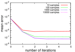
(b) as20000102

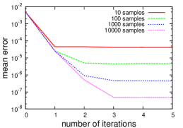
(c) wiki-Vote

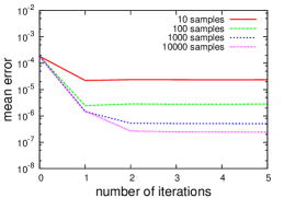
(d) ca-HepTh

Figure 2.1: Number of iterations $L$ vs. mean error of computed SimRank.

2.4.2 Efficiency

We next evaluate the efficiency of our algorithm. We first performed preprocessing with parameters $R=100$ and $L=3$, respectively. We then performed single-pair, single-source and all-pairs queries for real networks. Results are shown in Table 3.7.2; we omitted results of the all-pairs computation for a network larger than in-2004 since runtimes exceeded three days. We summarize our results below.

• For small networks ($n\leq 1,000,000$), only a few minutes of preprocessing time were required; furthermore, answers to single-pair queries were obtained in 100 milliseconds, while answers to single-source queries were obtained in 300 milliseconds. This efficiency is certainly acceptable for online services. We were also able to solve all-pairs query in a few days.

• For large networks, $n\geq 40,000,000$, a few hours of preprocessing time were required; furthermore, answers to single-pair queries were obtained approximately in 10 seconds, while answers to single-source queries were obtained in a half minutes. To the best of our knowledge, this is the first time that such an algorithm is successfully scaled up to such large networks.

• The space complexity is proportional to the number of edges, which enables us to compute SimRank values for large networks.

Computational results of our proposed algorithm and existing algorithms; single-pair and single-source results are the average of 10 trials; we omitted results of the all-pairs computation of our proposed algorithm for a network larger than in-2004 since runtimes exceeded three days; other omitted results (—) mean that the algorithms failed to allocate memory. Dataset Proposed [Yu et al. (2012)] [Fogaras and Rácz (2005)] Preproc. SinglePair SingleSrc. AllPairs Memory AllPairs Memory Preproc. SinglePair SingleSrc. Memory ca-GrQc 842 ms 0.236 ms 2.080 ms 10.90 s 3 MB 2.97 s 69 MB 64.7 s 87.0 ms 288 ms 23.3 GB as20000102 96 ms 0.518 ms 0.812 ms 5.26 s 2 MB 0.13 s 8 MB 106 s 112 ms 262 ms 28.1 GB Wiki-Vote 187 ms 0.613 ms 5.26 ms 37.4 s 6 MB 8.74 s 143 MB 43.4 s 30.4 ms 42.5 ms 24.5 GB ca-HepTh 698 ms 0.493 ms 3.24 ms 39.0 s 4 MB 23.3 s 316 MB 205 s 61.2 ms 262 ms 44.2 GB email-Enron 2.75 s 2.56 ms 24.13 ms 885 s 20 MB 302 s 3.47 GB 8055 s 86.9 ms 1.19 ms 162 GB soc-Epinions1 4.12 s 5.90 ms 74.4 ms 5647 s 31 MB 777 s 6.94 GB — — — — soc-Slashdot0811 6.14 s 4.16 ms 20.4 ms 1581 s 47 MB 747 s 7,37 GB — — — — soc-Slashdot0902 5.87 s 4.63 ms 21.0 ms 1725 s 49 MB 694 s 7.24 GB — — — — email-EuAll 11.3 s 14.5 ms 61.7 ms 4.54 h 57 MB 2.00 h 59.1 GB — — — — web-Stanford 21.0 s 9.76 ms 288 ms 22.5 h 132 MB — — — — — — web-NotreDame 8.07 s 14.7 ms 47.3 ms 4.28 h 107 MB 1.50 h 45.5 GB — — — — web-BerkStan 49.6 s 35.7 ms 272 ms 51.7 h 392 MB — — — — — — web-Google 52.2 s 64.2 ms 234 ms 57.0 h 325 MB 11.1 h 203 GB — — — — dblp-2011 104 s 53.6 ms 207 ms 53.7 h 395 MB 3140 s 24.1 GB — — — — in-2004 71.7 s 91.1 ms 335 ms — 843 MB — — — — — — flickr 160 s 137 ms 424 ms — 1.11 GB — — — — — — soc-LiveJournal 819 s 394 ms 1.19 s — 3.74 GB — — — — — — indochina-2004 391 s 487 ms 1.73 s — 8.15 GB — — — — — — it-2004 2822 s 3.51 s 12.0 s — 49.2 GB — — — — — — twitter-2010 14376 s 3.17 s 11.9 s — 59.4 GB — — — — — — uk-2007-05 8291 s 9.42 s 32.7 s — 153 GB — — — — — —

2.4.3 Comparisons with existing algorithms

In this section, we compare our algorithm with two state-of-the-art algorithms for computing SimRank. We used the same parameters ($R=100$, $L=3$) as the above.

Comparison with the state-of-the-art all-pairs algorithm

Yu et al. [Yu et al. (2012)] proposed an efficient all-pairs algorithm; the time complexity of their algorithm is $O(Tnm)$, and the space complexity is $O(n^{2})$. They computed SimRank via matrix-based iteration (2.1) and reduced the space complexity by discarding entries in SimRank matrix that are smaller than a given threshold. We implemented their algorithm and evaluated it in comparison with ours. We used the same parameters presented in [Yu et al. (2012)] that attain the same accuracy level as our algorithm.

Results are shown in Table 3.7.2; the omitted results (—) mean that their algorithm failed to allocate memory. From the results, we observe that their algorithm performs a little faster than ours, because the time complexity of their algorithm is $O(Tnm)$, whereas the time complexity of our algorithm is $O(T^{2}nm)$; however, our algorithm uses much less space. In fact, their algorithm failed for a network with $n\geq$ 300,000 vertices because of memory allocation. More importantly, their algorithm cannot estimate the memory usage before running the algorithm. Thus, our algorithm significantly outperforms their algorithm in terms of scalability.

Comparison with the state-of-the-art single-pair and single-source algorithm

Fogaras and Rácz [Fogaras and Rácz (2005)] proposed an efficient single-pair algorithm that estimates SimRank scores by using first meeting time formula (1.4) with Monte Carlo simulation. Like our approach, their algorithm also consists of two phases, a preprocessing phase and a query phase. In the preprocessing phase, their algorithm generates $R^{\prime}$ random walks and stores the walks efficiently; this phase requires $O(nR^{\prime})$ time and $O(nR^{\prime})$ space. In the query phase, their algorithm computes scores via formula (1.4); this phase requires $O(TnR^{\prime})$ time. We implemented their algorithm and evaluated it in comparison with ours.

We first checked the accuracy of their algorithm by computing all-pairs SimRank for the smaller datasets used in Section 2.4.1; results are shown in Table 2.4.3. From the table, we observe that in order to obtain the same accuracy as our algorithm, their algorithm requires $R^{\prime}\geq$ 100,000 samples, which are much larger than our random samples $R=100$. This is because their algorithm estimates all $O(n^{2})$ entries by Monte Carlo simulation, but our algorithm only estimates $O(n)$ diagonal entries by Monte Carlo simulation.

We then evaluated the efficiency of their algorithm with $R^{\prime}=$ 100,000 samples. These results are shown in Table 3.7.2. This shows that their algorithm needs much more memory, thus it only works for small networks. This concludes that in order to obtain accurate scores, our algorithm is much more efficient than their algorithm.

Accuracy of the single-pair algorithm proposed by Fogaras and Rácz [Fogaras and Rácz (2005)]; accuracy is shown as mean error. Dataset Samples Accuracy ca-GrQc 100 1.59 $\times 10^{-4}$ 1,000 5.87 $\times 10^{-5}$ 10,000 1.32 $\times 10^{-5}$ 100,000 6.43 $\times 10^{-6}$ (Proposed 4.77 $\times 10^{-6}$) as20000102 100 2.51 $\times 10^{-3}$ 1,000 7.87 $\times 10^{-4}$ 10,000 2.54 $\times 10^{-4}$ 100,000 8.69 $\times 10^{-5}$ (Proposed 1.19 $\times 10^{-7}$) wiki-Vote 100 1.03 $\times 10^{-3}$ 1,000 3.57 $\times 10^{-4}$ 10,000 1.13 $\times 10^{-4}$ 100,000 3.63 $\times 10^{-5}$ (Proposed 2.81 $\times 10^{-6}$) ca-HepTh 100 1.36 $\times 10^{-4}$ 1,000 5.58 $\times 10^{-5}$ 10,000 1.18 $\times 10^{-5}$ 100,000 6.04 $\times 10^{-6}$ (Proposed 4.56 $\times 10^{-6}$)

3 Top k-computation¹

3.1 Motivation and overview

In the previous section, we describe the SimRank linearization technique and show how to use the linearization to solve single-pair, single-source, and all-pairs SimRank problems. In this section, we consider an top $k$ search problem; we are given a vertex $i$ and then find $k$ vertices with the $k$ highest SimRank scores with respect to $i$. This problem is interested in many applications because, usually, highly similar vertices for a given vertex $i$ are very few (e.g., 10–20), and in many applications, we are are only interested in such highly similar vertices. This problem can be solved in $O(T^{2}m)$ time by using the single-source SimRank algorithm; however, since we only need $k$ highly-similar vertices, we can develop more efficient algorithm.

Here, we propose a Monte-Carlo algorithm based on SimRank linearization for this problem; the complexity is independent of the size of networks. Note that Fogaras and Racz [Fogaras and Rácz (2005)] also proposed the Monte-Carlo based single-pair computation algorithm. By comparing their algorithm, our main ingredients is the “pruning technique” by utilizing the SimRank linearization. We observe that SimRank score $s(i,j)$ decays very rapidly as distance of the pair $i,j$ increases. To exploit this phenomenon, we establish upper bounds of SimRank score $s(i,j)$ that only depend on distance $d(i,j)$. The upper bounds can be efficiently computed by Monte-Carlo simulation (in our preprocess). These upper bounds, together with some adaptive sample technique, allow us to effectively prune the similarity search procedure.

Overall, the proposed algorithm runs as follows.

1. We first perform preprocess to compute the auxiliary values for upper bounds of SimRank $s(i,j)$ for all $i\in V$ (see Section 3.4). In addition, we construct an auxiliary bipartite graph $H$, which allows us to enumerate “candidates” of highly similar vertices $j$ more accurate. This is our preprocess phase. The time complexity is $O(n)$.

2. We now perform our query phase. We compute SimRank scores $s(i,j)$ by the Monte-Carlo simulation for each vertex $i$ in the ascending order of distance from a given vertex $i$, and at the same time, we perform “pruning” by the upper bounds. We also combine the adaptive sampling technique for the Monte-Carlo simulation; specifically, for a query vertex $i$, we first estimate SimRank scores roughly for each candidate $j$ by using a small number of Monte-Carlo samples, and then we re-compute more accurate SimRank scores for each candidate $j$ that has high estimated SimRank scores.

3.2 Monte Carlo algorithm for single-pair SimRank

Let us consider a random walk that starts from $i\in V$ and that follows its in-links, and let $i^{(t)}$ be a random variable for the $t$-th position of this random walk. Then we observe that

$$P^{t}e_{i}=\mathbb{E}[e_{i^{(t)}}].$$ (3.1)

Therefore, by plugging (3.1) to (2.2.1), we obtain

$$s^{(T)}(i,j)= D_{ij}+c\mathbb{E}[e_{i^{(1)}}]^{\top}D\mathbb{E}[e_{j^{(1)}}]$$

$$+\cdots+c^{T-1}\mathbb{E}[e_{i^{(T-1)}}]^{\top}D\mathbb{E}[e_{j^{(T-1)}}].$$ (3.2)

Our algorithm computes the expectations in the right hand side of (3.2) by Monte-Carlo simulation as follows: Consider $R$ independent random walks $i^{(t)}_{1},\ldots,i^{(t)}_{R}$ that start from $i\in V$, and $R$ independent random walks $j^{(t)}_{1},\ldots,j^{(t)}_{R}$ that start from $j\in V$ with $i\neq j$. Then each $t$-th term of (3.2) can be estimated as

$$c^{t}\mathbb{E}[e_{i^{(t)}}]^{\top}D\mathbb{E}[e_{j^{(t)}}]\simeq\frac{c^{t}}{R^{2}}\sum_{r=1}^{R}\sum_{r^{\prime}=1}^{R}D_{i_{r}^{(t)}j_{r^{\prime}}^{(t)}}.$$ (3.3)

We compute the right hand side of (3.3). Specifically by maintaining the positions of $i_{1}^{(t)},\ldots,i_{R}^{(t)}$ and $j_{1}^{(t)},\ldots,j_{R}^{(t)}$ by hash tables, it can be evaluated in $O(R)$ time. Therefore the total time complexity to evaluate (3.2) is $O(TR)$. The algorithm is shown in Algorithm 6. We emphasize that this time complexity is independent of the size of networks (i.e, $n,m$) Hence this algorithm can scale to very large networks.

Algorithm 6 Monte-Carlo Single-pair SimRank

1:procedure SinglePair($i$,$j$)

2:     $i_{1}\leftarrow i,\ldots,i_{R}\leftarrow i$, $j_{1}\leftarrow j,\ldots,j_{R}\leftarrow j$

3:     $\sigma=0$

4:     for $t=0,1,\ldots,T-1$ do

5:         for $w\in\{i_{1},\ldots,i_{R}\}\cap\{i_{1}\ldots,i_{R}\}$ do

6:              $\alpha\leftarrow\#\{r:i_{r}=w,r=1,\ldots,R\}$

7:              $\beta\leftarrow\#\{r:j_{r}=w,r=1,\ldots,R\}$

8:              $\sigma\leftarrow\sigma+c^{t}D_{ww}\alpha\beta/R^{2}$

9:         end for

10:         for $r=1,\ldots,R$ do

11:              $i_{r}\leftarrow\delta_{-}(i_{r})$, $j_{r}\leftarrow\delta_{-}(j_{r})$, randomly

12:         end for

13:     end for

14:     return $\sigma$

15:end procedure

We give estimation of the number of samples to compute (3.2) accurately, with high probability. We use the Hoeffding inequality to show the following.

Proposition 3.1.

Let $\tilde{s}^{(T)}(i,j)$ be the output of the algorithm. Then

$$\mathbb{P}\left\{|\tilde{s}^{(T)}(i,j)-s^{(T)}(i,j)|\geq\epsilon\right\}\leq 4nT\exp\left(-\epsilon^{2}R/2(1-c)^{2}\right).$$ (3.4)

Lemma 3.2.

$$\mathbb{P}\left\{\left|X_{u}^{(t)\top}DX_{v}^{(t)}-(P^{t}e_{u})^{\top}DP^{t}e_{v}\right|\geq\epsilon\right\}\leq 4n\exp(-\epsilon^{2}R/2).$$

Proof 3.3.

$$\mathbb{P}\left\{\left|X_{u}^{(t)\top}DX_{v}^{(t)}-(P^{t}e_{u})^{\top}DP^{t}e_{v}\right|\geq\epsilon\right\}$$

$$\leq\mathbb{P}\left\{\left|X_{u}^{(t)\top}D\left(X_{v}^{(t)}-P^{t}e_{v}\right)\right|\geq\epsilon/2\right\}$$

$$+\mathbb{P}\left\{\left|\left(X_{u}^{(t)}-P^{t}e_{u}\right)^{\top}DP^{t}e_{v}\right|\geq\epsilon/2\right\}$$

$$\leq 4n\exp(-\epsilon^{2}R/2).$$

Proof 3.4 (of Proposition 3.1).

By Lemma 5.22, we have

$$\mathbb{P}\left\{\left|\left(\sum_{t=0}^{T-1}c^{t}X_{u}^{(t)\top}DX_{v}^{(t)}\right)-s^{(T)}(u,v)\right|\geq\epsilon\right\}$$

$$\leq \sum_{t=0}^{T-1}\mathbb{P}\left\{\left|c^{t}X_{u}^{(t)\top}DX_{v}^{(t)}-c^{t}(P^{t}e_{u})^{\top}DP^{t}e_{v}\right|\geq c^{t}\epsilon/(1-c)\right\}$$

$$\leq 4nT\exp\left(-\epsilon^{2}R/2(1-c)^{2}\right).$$

By Proposition 3.1, we have the following.

Corollary 3.5.

Algorithm 6 computes the SimRank score $s^{(T)}(u,v)$ with accuracy $0<\epsilon<1$ with probability $0<\delta<1$ by setting $R=2(1-c)^{2}\log(4nT/\delta)/\epsilon^{2}$.

3.3 Distance correlation of SimRank

Our top $k$ similarity search algorithm performs single-pair SimRank computations for a given source vertex $i$ and for other vertices $j$, but we save the time complexity by pruning. In order to perform this pruning, we need some upper bounds. This section and the next section are devoted to establish the upper bounds.

The important observation of SimRank is

SimRank score $s(i,j)$ decays very fast as the pair $i,j$ goes away.

In this section, we empirically verify this fact in some real networks, and in the next section, we develop the upper bounds that only depend on distance.

Let us look at Figure 3.1. We randomly chose 100 vertices $i$ and enumerate top-1000 similar vertices with respect to to a query vertex $u$ (note that these top-1000 vertices are “exact”, not ‘approximate”). Each point denotes the average distance of the $k$-th similar vertex. To convince the reader, we also give the average distance between two vertices for each network by the blue line.

Figure 3.1 clearly shows much intuitive information. If we only need to compute top-10 vertices, all of them are within distance two, three, or four. In real applications, it is unlikely that we need to compute top-1000 vertices, but even for this case, most of them are within distance four or five. We emphasize that these distances are smaller than the average distance of two vertices in each network. Thus we can conclude that the “candidates” of highly similar vertices are screened by distances very well.

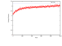
wiki-Vote

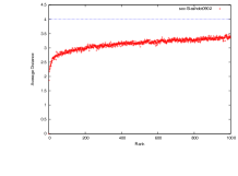
soc-Slashdot0902

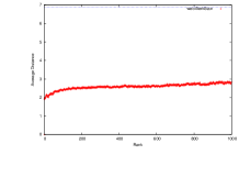
web-BerkStan

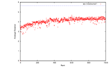
soc-LiveJournal1

Figure 3.1: Distance correlation of similarity ranking. The red points are for distance of top-1000 similar vertices and the blue line is for average distance of two vertices in each network

There is one remark we would like to make from Figure 3.1. The top-10 highest SimRank vertices in Web graphs are much closer to a query vertex than social networks. Thus we can also claim that our algorithm would work better for Web graphs than for social networks, because we only look at subgraphs induced by vertices of distance within three (or even two) from a query vertex. This claim is verified in Section 3.6.

3.4 Tight upper bounds

In the previous section, we observe that highly similar vertices with respect to a query vertex are within small distance from $u$. This observation allows us to propose our efficient algorithm for the top-$k$ similarity search problem for a single vertex. In order to obtain this algorithm, we need to establish the upper bounds of SimRank that depend only on distance, which will be done in this section.

Let us observe that by definition, SimRank score is bounded by the decay factor to the power of the distance:

$$s(u,v)\leq c^{d(u,v)}$$

Since almost all high SimRank score vertices with respect to a query vertex $u$ are located within distance three from $u$ (see Figure 3.1), we obtain $s(u,v)\leq c^{3}=0.216$. But this is too large for our purpose (indeed, our further experiments to compare actual SimRank scores with this bound confirm that it is too large).

Here we propose two upper bounds, called “L1 bound” and “L2 bound”. Our algorithm, described in a later section, combines these two bounds to perform “pruning”, which results in a much faster algorithm.

3.4.1 L1 bound

The first bound is based on the following inequality: for a vector $x$ and a stochastic vector $y$,

$$x^{\top}y\leq\max_{w\in\mathrm{supp}(y)}x^{\top}e_{w},$$ (3.5)

where $\mathrm{supp}(y):=\{w\in V:y(w)>0\}$ is a positive support of $y$. We bound $(P^{t}e_{u})^{\top}D(P^{t}e_{v})$ by this inequality.

Fix a query vertex $u$. Let us define

$$\alpha(u,d,t):=\max_{w\in V,d(u,w)=d}(P^{t}e_{u})^{\top}De_{w}$$ (3.6)

for $d=1,\ldots,d_{\mathrm{max}}$ and $t=1,\ldots,T$, and

$$\beta(u,d):=\sum_{t=0}^{T-1}c^{t}\max_{d-t\leq d^{\prime}\leq d+t}\alpha(u,d^{\prime},t)$$ (3.7)

for $t=1,\ldots,T$. Here $d_{\mathrm{max}}$ is distance such that if $d(u,v)>d_{\mathrm{max}}$ then $s(u,v)$ is too small to take into account. (We usually set $d_{\mathrm{max}}=T$).

Proposition 3.6.

For a vertex $v$ with $d(u,v)=d$, we have

$$s^{(T)}(u,v)\leq\beta(u,d)$$ (3.8)

The proof will be given in Appendix.

Remark 3.7.

$\alpha(u,d,t)$ has the following probabilistic representation:

$$\alpha(u,d,t)=\max_{d(u,w)=d}D_{ww}\mathbb{P}\{u^{(t)}=w\}$$

where $u^{(t)}$ denotes the position of a random walk that starts from $u$ and follows its in-links.

To compute $\alpha(u,d,t)$ and $\beta(u,d)$, we can use Monte-Carlo simulation for $P^{t}e_{u}$ as shown in Algorithm 7.

Similar to Proposition 3.1, we obtain the following proposition, whose proof will be given in Appendix. This proposition shows that Algorithm 7 can compute $\alpha(u,d,t)$ and $\beta(u,d)$.

Proposition 3.8.

Let $\tilde{\beta}(u,d)$ be computed by Algorithm 7. Then

$$\mathbb{P}\left\{|\tilde{\beta}(d,t)-\beta(d,t)|\geq\epsilon\right\}\leq 2nd_{\mathrm{max}}T\exp(-2\epsilon^{2}R)$$

By Proposition 3.8, we have the following.

Corollary 3.9.

Algorithm 7 computes $\beta(u,d)$ with accuracy less than $0<\epsilon<1$ with probability at least $0<\delta<1$ by setting $R=\log(2nd_{\mathrm{max}}T/\delta)/(2\epsilon^{2})$.

Algorithm 7 Monte-Carlo $\alpha(u,d,t)$, $\beta(u,d)$ computation

1:procedure ComputeAlphaBeta($u$)

2:     $u_{1}\leftarrow u,\ldots,u_{R}\leftarrow u$

3:     for $t=0,1,\ldots,T-1$ do

4:         for $w\in\{u_{1},\ldots,u_{R}\}$ do

5:              $\mu\leftarrow D_{ww}\#\{r:u_{r}=w,r\in[1,R]\}/R$

6:              $\alpha(u,d(u,w),t)\leftarrow\max\{\alpha(u,d(u,w),t),\mu\}$

7:         end for

8:         for $r=1,\ldots,R$ do

9:              $u_{r}\leftarrow\delta(u_{r})$ randomly

10:         end for

11:     end for

12:     for $d=1,\ldots,T$ do

13:         $\beta(u,d)=\sum_{t=0}^{T-1}c^{t}\max_{d-t\leq d^{\prime}\leq d+t}\alpha(u,d^{\prime},t)$

14:     end for

15:end procedure

3.4.2 L2 bound

The second bound is based on the Cauchy–Schwartz inequality: for nonnegative vectors $x$ and $y$,

$$x^{\top}y\leq\|x\|\|y\|.$$ (3.9)

We also bound $(P^{t}e_{u})D(P^{t}e_{v})$ by this inequality.

Let

$$\gamma(u,t):=\|\sqrt{D}P^{t}e_{u}\|,$$ (3.10)

where $\sqrt{D}=\mathrm{diag}(\sqrt{D_{11}},\ldots,\sqrt{D_{nn}})$. Note that, since $D$ is a nonnegative diagonal matrix, $\sqrt{D}$ is well-defined.

Proposition 3.10.

For two vertices $u$ and $v$, we have

$$s^{(T)}(u,v)\leq\sum_{t=0}^{T}c^{t}\gamma(u,t)\gamma(v,t)$$ (3.11)

The proof of Proposition 3.10 will be given in Appendix.

To compute $\gamma(u,d)$ for each $u$, we can use Monte-Carlo simulation. Let us emphasize that we can compute $\gamma(u,d)$ for each $u$ and $d\leq d_{\mathrm{max}}$ in preprocess.

The following proposition, whose proof will be given in Appendix, shows that Algorithm 8 can compute $\gamma(u,d)$.

Proposition 3.11.

Let $\tilde{\gamma}(u,t)$ be computed by Algorithm 8. Then

$$\mathbb{P}\left\{|\tilde{\gamma}(u,t)-\gamma(u,t)|\geq\epsilon\right\}\leq 4n\exp\left(-\epsilon^{2}R/8\right).$$

The proof of of Proposition 3.11 will be given in Appendix. By Proposition 3.11, we have the following.

Corollary 3.12.

Algorithm 8 computes $\gamma(u,t)$ with accuracy less than $0<\epsilon<1$ with probability at least $0<\delta<1$ by setting $R=8\log(4n/\delta)/\epsilon^{2}$.

Algorithm 8 Monte-Carlo $\gamma(u,t)$ computation

1:procedure ComputeGamma($u$)

2:     $u_{1}\leftarrow u,\ldots,u_{R}\leftarrow u$

3:     for $t=0,1,\ldots,T-1$ do

4:         $\mu=0$

5:         for $w\in\{u_{1},\ldots,u_{R}\}$ do

6:              $\mu\leftarrow\mu+D_{ww}\#\{r:u_{r}=w,r\in[1,R]\}^{2}/R^{2}$

7:         end for

8:         $\gamma(u,t)\leftarrow\sqrt{\mu}$

9:         for $r=1,\ldots,R$ do

10:              $u_{r}\leftarrow\delta(u_{r})$ randomly

11:         end for

12:     end for

13:end procedure

3.4.3 Comparison of two bounds

The reason why we need both L1 and L2 bounds is the following: The L1 bound is more effective for a low degree query vertex $u$. This is because if $u$ has low degree then $P^{t}e_{u}$ is sparse. Therefore the bound (5.7) becomes tighter.

On the other hand, the L2 bound is more effective for high degree vertex $u$. This is because if $u$ has high degree then $P^{t}e_{u}$ spreads widely, and hence each entry is small. Therefore $\|\sqrt{D}P^{t}e_{u}\|$ decrease rapidly.

3.5 Algorithm

We are now ready to provide our whole algorithm for top-$k$ similarity search. Our algorithm consists of two phases: preprocess phase and query phase. In the query phase, for a given vertex $u$, we compute single-pair SimRanks $s(u,v)$ for some vertices $v$ that may have high SimRank value (we call such vertices candidates that are computed in the preprocess phase), and output $k$ highly similar vertices.

In order to obtain similar vertices accurately, we have to perform many Monte Carlo simulations in single-pair SimRank computation (Algorithm 6). Thus, the key of our algorithm is the way to reduce the number of candidates that are computed in the preprocess phase in Section 7.1.

3.5.1 Preprocess phase

In the preprocess phase, we precompute $\gamma$ in (3.10) for the L2 bound as described in Algorithm 8. Note that we compute $\alpha,\beta$ in (3.6), (3.7) for the L1 bound in query phase.

After that, for each vertex $u$, we enumerate “candidates” of highly similar vertices $v$. For this purpose, we consider the following auxiliary bipartite graph $H$. The left and right vertices of $H$ are copy of $V$ (i.e., $H$ has $2n$ vertices). Let $u_{\mathrm{left}}$ be the copy of $u\in V$ in the left vertices and let $v_{\mathrm{right}}$ be the copy of $v\in V$ in the right vertices. There is an edge $(u_{\mathrm{left}},v_{\mathrm{right}})$ if a random walk that starts from $u$ frequently reaches $v$. By this construction, a pair of vertices $u$ and $v$ has high SimRank score if $u_{\mathrm{left}}$ and $v_{\mathrm{left}}$ share many neighbors. We construct this bipartite graph $H$ by performing Monte-Carlo simulations in the original graph $G$ as follows. For each vertex $u$, we iterate the following procedure $P$ times to construct an index for $u$. We perform a random walk $W_{0}$ of length $T$ from $u$ in $G$. We further perform $Q$ random walks $W_{1},\ldots,W_{Q}$ from $u$. Let $v$ be $t$-th vertex on $W_{0}$. Then we put an edge $(u_{\mathrm{left}},v_{\mathrm{right}})$ in $H$ if there are at least two random walks in $W_{1},\dots W_{Q}$ that contain $v$ at $t$-th step. The whole procedure is described in Algorithm 3 below. Here, for a random walk $W_{j}$ and $t\geq 0$, we denote the vertex at the $t$-th step of $W_{j}$ by $W_{jt}$.

In our experiment, we set $P=10$, $T=11$ and $Q=5$. The time complexity of this preprocess phase is $O(n(R+PQ)T)$, where $R$ comes from Algorithm 3 and we set $R=100$ in our experiment. The space complexity is $O(nP)$, but in practice, since the number of candidates are usually small, the space is less smaller than this bound.

Algorithm 9 Proposed algorithm (preprocess)

1:procedure Indexing

2:     for $u\in V$ do

3:         for $i=1,\ldots,P$ do

4:              Perform a random walk $W_{0}$ from $u$

5:              Perform random walks $W_{1}$,$\ldots$,$W_{Q}$ from $u$

6:              for $t=1,\ldots,T$ do

7:                  if $W_{jt}=W_{kt}$ for some $j\neq k$ then

8:                       Add $W_{0t}$ for index of $u$

9:                  end if

10:              end for

11:         end for

12:     end for

13:end procedure

3.5.2 Query phase

We now describe our query phase. For a given vertex $u$, we first traverse the auxiliary bipartite graphs $H$ and enumerate all the vertices $v$ that share the neighbor in $H$. We then prune some vertices $v$ by L1 and L2 bounds. After that, for each candidate $v$, we compute SimRank scores $s(u,v)$ by Algorithm 6. Finally we output top $k$ similar vertices as the solution of similarity search.

To accelerate the above procedure, we use the adaptive sample technique. For a query vertex $u$, we first set $R=10$ (in Algorithm 6) and estimate SimRank scores roughly for each candidate $v$ by Monte Carlo simulation (i.e, we only perform 10 random walks for $v$ by Algorithm 6). Then, we change $R=100$ and re-compute more accurate SimRank scores for each candidate $v$ that has high estimated SimRank scores by Monte Carlo simulation (i.e, we perform 100 random walks for $v$ by Algorithm 6). The whole procedure is described in Algorithm 5.

The overall time complexity of the query phase is $O(RT|S|)$ where $|S|$ is the number of candidates, since computing SimRank scores $s(u,v)$ by Algorithm 6 for two vertices $u,v$ takes $O(RT)$. The space complexity is $O(m+nP)$.

Algorithm 10 Proposed algorithm (query)

1:procedure Query($u$)

2:     Enumerate $S:=\{v|\delta_{H}(u_{\mathrm{left}})\cap\delta_{H}(v_{\mathrm{left}})\neq\emptyset\}$

3:     Prune $S$ by L1 and L2 bound

4:     for $v\in S$ do

5:         Perform Algorithm 6 $R=10$ times to roughly estimate $s(u,v)$.

6:         if The estimated score $s(u,v)$ is not small then

7:              Perform Algorithm 6 $R=100$ times to estimate $s(u,v)$ more accurately

8:         end if

9:     end for

10:     Output top $k$ similar vertices

11:end procedure

3.6 Experiment

We perform our proposed algorithm for several real networks and evaluate performance of our algorithm. We also compare our algorithm with some state-of-the-art algorithms.

All experiments are conducted on an Intel Xeon E5-2690 2.90GHz CPU with 256GB memory and running Ubuntu 12.04. Our algorithm is implemented in C++ and compiled with g++v4.6 with -O3 option.

According to discussion in the previous section, we set the parameters as follows: decay factor $c=0.6$, $T=11$, $R=100$ for $\gamma$ (Algorithm 8) and for $s(\cdot,\cdot)$ (Algorithm 6), and $R=10000$ for $\alpha$ and $\beta$ (Algorithm 7) that is optimized by pre-experiment. We also set $P=10$, $T=11$ and $Q=5$ in our preprocess phase as in Section 7.1.

In addition, we set $k=20$ since we are only interested in small number of similar vertices. To avoid searching vertices of very small SimRank scores, we set a threshold $\theta=0.01$ to terminate the procedure when upper bounds become smaller than $\theta$.

We use the datasets shown in Table 2.4.

3.7 Results

We evaluate our proposed algorithm for several real networks. The results are summarized in Tables 3.7.2.

We first observe that our proposed algorithm can find top-20 similar vertices in less than a few seconds for graphs of billions edges (i.e., “it-2004”) and in less than a second for graphs of one hundred millions edges, respectively.

We can also observe that the query time for our algorithm does not much depend on the size of networks. For example, “indochina-2004” has 8 times more edges than “flickr” but the query time is twice faster than that. Hence the computational time of our algorithm depends on the network structure rather than the network size. Specifically, our algorithm works better for web graphs than for social networks.

3.7.1 Analysis of Accuracy

In this subsection, we shall investigate performance of our algorithm in terms of accuracy. In many applications, we are only interested in very similar vertices. Hence we only look at vertices that have high SimRank scores.

Specifically, what we do is the following. We first compute, for a query vertex $u$, the single source SimRank scores $s(u,v)$ for all the vertices $v$ (for the whole graph) by the exact method. Then we pick up all “high score” vertices $v$ with score at least $t$ from this computation (for $t=0.04$, $0.05$, $0.06$, $0.07$). Finally, we compute “high score” vertices $v$ with respect to the query vertex $u$ by our proposed algorithm. Let us point out that our algorithm can be easily modified so that we only output high SimRank score vertices(because we just need to set up the threshold to prune the similarity search). We then compute the following value:

$$\frac{\textrm{\# of our high score vertices}}{\textrm{\# of the optimal high score vertices}}.$$

We also do the same thing for high score vertices computed by Fogaras and Rácz [Fogaras and Rácz (2005)](we used the same parameter $R^{\prime}=100$ presented in [Fogaras and Rácz (2005)]). We perform this operation 100 times, and take the average. The result is in Table 3.7.2. We can see that our algorithm actually gives very accurate results. In addition, our algorithm gives better accuracy than Fogaras and Rácz [Fogaras and Rácz (2005)].

3.7.2 Comparison with existing results

In this subsection, we compare our algorithm with two state-of-the-art algorithms for computing SimRank, and show that our algorithm outperforms significantly in terms of scalability.

Comparison with the state-of-the-art all-pairs algorithm

Yu et al. [Yu et al. (2012)] proposed an efficient all-pairs algorithm; the time complexity of their algorithm is $O(Tnm)$, and the space complexity is $O(n^{2})$, where $T$ is the number of the iterations. We implemented their algorithm and evaluated it in comparison with ours. We used the same parameters presented in [Yu et al. (2012)].

Results are shown in Table 3.7.2; the omitted results (—) mean that their algorithm failed to allocate memory. From the results, we observe that their algorithm is a little faster than ours in query time, but our algorithm uses much less space(15–30 times). In fact, their algorithm failed for graphs with a million edges, because of memory allocation. More importantly, their algorithm cannot estimate the memory usage before running the algorithm. Moreover, since our all-pairs algorithm can easily be parallelized to multiple machines, if there are 100 machines, even for graphs of billions size, our all-pairs algorithm can output all top-20 vertices in less than 5 days. Thus, our algorithm significantly outperforms their algorithm in terms of scalability.

Comparison with the state-of-the-art single-pair and single-source algorithm

Fogaras and Rácz [Fogaras and Rácz (2005)] proposed an efficient single-pair algorithm that estimates SimRank scores with Monte Carlo simulation. Like our approach, their algorithm also consists of two phases, a preprocessing phase and a query phase. In the preprocessing phase, their algorithm generates $R^{\prime}$ random walks and stores the walks efficiently; this phase requires $O(nR^{\prime})$ time and $O(nR^{\prime})$ space. The query phase phase requires $O(TnR^{\prime})$ time, where $T$ is the number of iterations. We implemented their algorithm and evaluated it in comparison with ours. We used the same parameter $R^{\prime}=100$ presented in [Fogaras and Rácz (2005)].

We can see that their algorithm is faster in query time. But we suspect that this is due to relaxing accuracy, as in the previous subsection. In order to obtain the same accuracy as our algorithm, we suspect that $R^{\prime}$ should be 500–1000, which implies that their algorithm would be at least 5–10 times slower, and require at leats 5–10 times more space.

In this case, their algorithm would fail for graphs with more than ten millions edges because of memory allocation. Even for the case $R^{\prime}=100$, our algorithm uses much less space(10–20 times), and their algorithm failed for graphs with more than 70 millions edges because of memory allocation. Therefore we can conclude that our algorithm significantly outperforms their algorithm in terms of scalability.

Accuracy. Dataset Threshold Proposed Fogaras and Rácz [Fogaras and Rácz (2005)] ca-GrQc 0.04 0.98665 0.92329 0.05 0.98854 0.92467 0.06 0.99461 0.95225 0.07 0.99554 0.92881 as20000102 0.04 0.97831 0.94643 0.05 0.98727 0.94783 0.06 0.99177 0.94713 0.07 0.99550 0.94760 wiki-Vote 0.04 0.81862 0.93491 0.05 0.88629 0.93760 0.06 0.90801 0.94215 0.07 0.94785 0.97916 ca-HepTh 0.04 0.97142 0.88964 0.05 0.98782 0.94354 0.06 0.99673 0.91848 0.07 0.99746 0.93647

Preprocess time, query time and space for our proposed algorithm, [Fogaras and Rácz (2005)], and [Yu et al. (2012)]. The single-pair and single-source results are the average of 10 trials; we omitted results of the all-pairs computation of our proposed algorithm for large networks; other omitted results (—) mean that the algorithms failed to allocate memory. Dataset Proposed [Fogaras and Rácz (2005)] [Yu et al. (2012)] Preproc. Query AllPairs Index Preproc. Query Index AllPairs Memory ca-GrQc 1.5 s 2.6 ms 13.5 s 2.4 MB 110 ms 0.11 ms 22.7 MB 2.97 s 66 MB as20000102 1.6 s 18 ms 115 s 3.3 MB 81 ms 1.3 ms 28.0 MB 0.13 s 51 MB Wiki-Vote 1.9 s 3.8 ms 26.9 s 5.3 MB 110 ms 0.41 ms 31.1 MB 8.74 s 138 MB ca-HepTh 1.8 s 3.3 ms 32.3 s 4.5 MB 253 ms 0.44 ms 43.3 MB 23.3 s 312 MB email-Enron 7.8 s 24 ms 864 s 21.6 MB 949 ms 1.1 ms 158 MB 302 s 3.45 GB soc-Epinions1 19.5 s 44 ms 3335 s 18.9 MB 1.8 s 1.4 ms 332 MB 777 s 6.91 GB soc-Slashdot0811 20.2 s 53 ms 4081 s 48.6 MB 1.9 s 1.2 ms 341 MB 747 s 7,34 GB soc-Slashdot0902 21.3 s 55 ms 4515 s 51.2 MB 2.0 s 1.3 ms 363 MB 694 s 7.21 GB email-EuAll 55.6 s 226 ms — 103 MB 3.6 s 14 ms 1.1 GB — — web-Stanford 69.6 s 103 ms — 141 MB 10.4 s 10 ms 1.2 GB — — web-NotreDame 60.6 s 73 ms — 163 MB 7.6 s 2.8 ms 1.4 GB — — web-BerkStan 240.2 s 93 ms — 288 MB 47.4 s 4.3 ms 3.8 GB — — web-Google 156.7 s 199 ms — 211 MB 24.0 s 13 ms 3.0 GB — — dblp-2011 82.2 s 16 ms — 144 MB 16.4 s 1.3 ms 1.4 GB — — in-2004 292.9 s 95 ms — 451 MB 46.4 s 6.8 ms 6.0 GB — — flickr 622.7 s 1.5 s — 513 MB 90.1 s 7.6 ms 7.4 GB — — soc-LiveJournal 2335.9 s 431 ms — 1.2 GB 397.9 s 27 ms 21.6 GB — — indochina-2004 1585.2 s 714 ms — 2.1 GB — — — — — it-2004 3.1 h 2.3 s — 11.2 GB — — — — — twitter-2010 7.7 h 17.4 s — 8.4 GB — — — — — —

4 SimRank join¹

4.1 Motivation and overview

Finally, in this section, we describe the SimRank join problem, which is formulated as follows.

Problem 4.1 (SimRank join).

Given a directed graph $G=(V,E)$ and a threshold $\theta\in[0,1]$, find all pairs of vertices $(i,j)\in V\times V$ for which the SimRank score of $(i,j)$ is greater than the threshold, i.e., $s(i,j)\geq\theta$,

This problem is useful in the near-duplication detection problem [Chen et al. (2002), Arasu et al. (2009)]. Let us consider the World Wide Web, which contains many “very similar pages.” These pages are produced by activities such as file backup, caching, spamming, and authors moving to different institutions. Clearly, these very similar pages are not desirable for data mining, and should be isolated from the useful pages by near-duplication detection algorithms.

Near duplication detection problem is solved by the similarity join query. Let $s(i,j)$ be a similarity measure, i.e., for two objects $i$ and $j$, they are (considered as) similar if and only if $s(i,j)$ is large. The similarity join query with respect to $s$ finds all pairs of objects $(i,j)$ with similarity score $s(i,j)$ exceeding some specified threshold $\theta$ [White and Jain (1996)]. The similarity join is a fundamental query for a database, and is used in applications, such as merge/purge [Hernández and Stolfo (1995)], record linkage [Fellegi and Sunter (1969)], object matching [Sivic and Zisserman (2003)], and reference reconciliation [Dong et al. (2005)].

Selecting the similarity measure $s(i,j)$ is an important component of the similarity join problem. Similarity measures on graphs have been extensively investigated. Here, we are interested in link-based similarity measures, which are determined by sorely the link structure of the network. For applications in the World Wide Web, by comparing content-based similarity measures, which are determined by the content data stored on vertices (e.g., text and images), link-based similarity measures are more robust against spam pages and/or machine-translated pages.

4.1.1 Difficulty of the problem

In solving the SimRank join problem, the following obstacles must be overcome.

1. There are many similar-pair candidates.

2. Computationally, SimRank is very expensive.

To clarify these issues, we compare the SimRank with the Jaccard similarity, where the Jaccard similarity between two vertices $i$ and $j$ is given by

$$J(i,j):=\frac{|{\delta}(i)\cap{\delta}(j)|}{|{\delta}(i)\cup{\delta}(j)|}.$$

Regarding the first issue, since the Jaccard similarity satisfies $J(i,j)=0$ for all pairs of vertices $(i,j)$ with $d(i,j)\geq 3$ (i.e., their distance is at least three), the number of possibly similar pairs (imposing the Jaccard similarity) is easily reduced to much smaller than all possible pairs. This simple but fundamental concept is adopted in many existing similarity join algorithms [Sarawagi and Kirpal (2004)]. However, since the SimRank exploits the information in multihop neighborhoods and hence scans the entire graph, it must consider all $O(n^{2})$ pairs, where $n$ is the number of vertices. Therefore, whereas the Jaccard similarity is adopted in “local searching,” the SimRank similarity must look at the global influence of all vertices, which requires tracking of all $O(n^{2})$ pairs.

Regarding the second issue, the Jaccard similarity of two vertices can be very efficiently computed (e.g., in $O(|{\delta}(i)|+|{\delta}(j)|)$ time using a straightforward method or in $O(1)$ time using MinHash [Broder (1997), Lee et al. (2011)]). Conversely, SimRank computation is very expensive.

Notably, until recently, most SimRank algorithms have computed the all-pairs SimRank scores [Jeh and Widom (2002), Lizorkin et al. (2010), Yu et al. (2010)], which requires at least $O(n^{2})$ time, and if we have the all-pairs SimRank scores, the SimRank join problem is solved in $O(n^{2})$ time. For example, in one investigation of the SimRank join problem [Zheng et al. (2013)], the all-pairs SimRank scores were first computed by an existing algorithm and an index for the SimRank join was then constructed. Therefore, developing scalable algorithm for the SimRank join problem is a newer challenging problem.

4.1.2 Contribution and overview

Here, we propose a scalable algorithm for the SimRank join problem, and perform experiments on large real datasets. The computational cost of the proposed algorithm only depends on the number of similar pairs, but does not depend on all pairs $O(n^{2})$. The proposed algorithm scales up to the network of 5M vertices and 70M edges. By comparing with the state-of-the-art algorithms, it is about 10 times faster, and requires about only 10 times smaller memory.

This section overviews our algorithm, which consists of two phases: filter and verification. The former enumerates the similar pair candidates, and then the latter decides whether each candidate pair is actually similar. Note that this framework is commonly adopted in similarity join algorithms [Xiao et al. (2011), Deng et al. (2014)]. A more precise description of the two phases is given below.

The filter phase is the most important phase of the proposed algorithm because it must overcome both (1) and (2) difficulties, discussed in previous subsection. We combines the following three techniques for this phase. The details are discussed in Section 4.2.

1. We adopt the SimRank linearization (Section 2) by which the SimRank is computed as a solution to a linear equation.

2. We solve the linear equation approximately by the Gauss-Southwell algorithm [Southwell (1940), Southwell (1946)], which avoids the need to compute the SimRank scores for non-similar pairs (Sections 4.2.1,4.2.2).

3. We adopt the stochastic thresholding to reduce the memory used in the Gauss-Southwell algorithm (Section 4.2.3).

The verification phase is simpler than the filter phase. We adopt the following two techniques for this phase. The details are discussed in Section 4.3.

1. We run a Monte-Carlo algorithm for each candidate to decide whether the candidate is actually similar. This can be performed in parallel.

2. We control the number of Monte-Carlo samples adaptively to reduce the computational time.

It should be emphasized that, we give theoretical guarantees for all techniques used in the algorithm. All omitted proofs are given in Appendix.

The proposed algorithm is evaluated by experiments on real datasets (Section 4.4). The algorithm is 10 times faster, and requires only 10 times smaller memory that of the state-of-the-arts algorithms, and scales up to the network of 5M vertices and 70M edges. Since the existing study [Zheng et al. (2013)] only performed in 338K vertices and 1045K edges, our experiment scales up to the 10 times larger network. Also, we empirically show that the all techniques used in the algorithm works effectively.

We also verified that the distribution of the SimRank scores on a real-world network follows a power-law distribution [Cai et al. (2009)], which has been verified only on small networks.

4.2 Filter phase

Algorithm 11 SimRank join algorithm.

1:procedure SimRankJoin($\theta$)

2:     Compute two sets $J_{L}$ and $J_{H}$.

3:     Output all $(i,j)\in J_{L}$.

4:     for $(i,j)\in J_{H}\setminus J_{L}$ do

5:         if $i$ and $j$ are really similar then

6:              Output $(i,j)$.

7:         end if

8:     end for

9:end procedure

In this section, we discuss the details of the filter phase for enumerating similar-pair candidates. We will discuss the details of the verification phase in the next section. Let us give overview of the filter phase.

Let $J(\theta)=\{(i,j):s(i,j)\geq\theta\}$ be the set of similar pairs. The filter phase produces two subsets $J_{L}(\theta,\gamma)$ and $J_{H}(\theta,\gamma)$ such that

$$J_{L}(\theta,\gamma)\subseteq J(\theta)\subseteq J_{H}(\theta,\gamma),$$ (4.1)

where $\gamma\in[0,1]$ is an accuracy parameter. Here, $J_{L}(\theta,\gamma)$ is monotone increasing in $\gamma$, $J_{H}(\theta,\gamma)$ is monotone decreasing in $\gamma$, and $J_{L}(\theta,1)=J(\theta)=J_{H}(\theta,1)$. Note that, our filter phase gives 100%-precision solution $J_{L}(\theta,\gamma)$ and 100%-recall solution $J_{H}(\theta,\gamma)$. These two sets might be useful in some applications.

Let us consider how to implement the filter phase. The basic idea is that “compute only relevant entries of SimRank.” In order to achieve this idea, we combine the two techniques, the linearization of the SimRank [Kusumoto et al. (2014), maehara2014efficient], and the Gauss-Southwell algorithm [Southwell (1940), Southwell (1946)] for solving a linear equation. The linearization of the SimRank is a technique to convert a SimRank problem to a linear equation problem. By using this technique, the problem of computing large entries of SimRank is transformed to the problem of computing large entries of a solution of a linear equation. To solve this linear algebraic problem, we can use the Guass-Southwell algorithm. By error analysis of the Guass-Southwell algorithm (given later in this paper), our filter algorithm obtains the lower and the upper bound of the SimRank of each pair $(i,j)$. Using these bounds, the desired sets $J_{L}(\theta,\gamma)$ and $J_{H}(\theta,\gamma)$ are obtained, where $\gamma$ is an accuracy parameter used in the Guass-Southwell algorithm.

The above procedure is already much efficient; however, we want to scale up the algorithm for large networks. The bottleneck of the above procedure is the memory allocation. We resolve this issue by introducing the stochastic thresholding technique.

This is the overview of the proposed filter phase. In the following subsections, we give details of the filter phase.

4.2.1 Gauss-Southwell algorithm

By the linearization of the SimRank, we obtained the linear equation (2.2). We want to solve this linear equation in $S$; however, since it has $O(n^{2})$ variables, we must keep track only on large entries of $S$. For this purpose, we adopt the Gauss-Southwell algorithm [Southwell (1940), Southwell (1946)], which is a very classical algorithm for solving a linear equation. In this subsection, we describe the Gauss-Southwell algorithm for a general linear equation $Ax=b$, and in the next subsection, we apply this method for the linearized SimRank equation (2.2).

Suppose we desire an approximate solution to the linear system $Ax=b$, where $A$ is an $n\times n$ matrix with unit diagonal entries, i.e., $A_{ii}=1$ for all $i=1,\ldots,n$. Let $\epsilon>0$ be an accuracy parameter. The Gauss-Southwell algorithm is an iterative algorithm. Let $x^{(t)}$ be the $t$-th solution and $r^{(t)}:=b-Ax^{(t)}$ be the corresponding residual. At each step, the algorithm chooses an index $i$ such that $|r^{(t)}_{i}|\geq\epsilon$, and updates the solution as

$$x^{(t+1)}=x^{(t)}+r^{(t)}_{i}e_{i},$$ (4.2)

where $e_{i}$ denotes the $i$-th unit vector. The corresponding residual becomes

$$r^{(t+1)}=b-Ax^{(t+1)}=r^{(t)}-r^{(t)}_{i}Ae_{i}.$$ (4.3)

Since $A$ has unit diagonals, the $i$-th entry of $r^{(t+1)}$ is zero. Repeating this process until $r^{(t)}_{i}<\epsilon$ for all $i=1,\ldots,n$, we obtain a solution $x$ such that $\|b-Ax\|_{\infty}<\epsilon$. This algorithm is called the Gauss-Southwell algorithm.

Note that this algorithm is recently rediscovered and applied to the personalized PageRank computation. See Section 1.2 for related work.

4.2.2 Filter phase

We now propose our filtering algorithm. First, we compute the diagonal correction matrix $D$ by Algorithm 4, reducing the SimRank computation problem to the linear equation (2.2). The Gauss-Southwell algorithm is then applied to the equation.

The $t$-th solution $S^{(t)}$ and the corresponding residual $R^{(t)}$ are maintained such that

$$D-(S^{(t)}-cP^{\top}S^{(t)}P)=R^{(t)}.$$ (4.4)

Initial conditions are $S^{(0)}=O$ and $R^{(0)}=D$. At each step, the algorithm finds an entry $(i,j)$ such that $|R^{(t)}_{ij}|\geq\epsilon$, and then updates the current solution as

$$S^{(t+1)}=S^{(t)}+R^{(t)}_{ij}e_{i}e_{j}^{\top}.$$ (4.5)

The corresponding residual becomes

$$R^{(t+1)}=R^{(t)}-R^{(t)}_{ij}e_{i}e_{j}^{\top}+cR^{(t)}_{ij}(P^{\top}e_{i})(P^{\top}e_{j})^{\top}.$$ (4.6)

Since we have assumed that $G$ is simple, the $i$-th entry of $P^{\top}e_{i}$ is zero, the $(i,j)$-th entry of $R^{(t+1)}$ is also zero. The algorithm repeats this process until $|R^{(t)}_{ij}|<\epsilon$ for all $i,j\in V$. The procedure is outlined in Algorithm 12.

Algorithm 12 Gauss-Southwell algorithm used in Algorithm 13.

1:procedure GaussSouthwell($\epsilon$)

2:     $S^{(0)}=O,\,R^{(0)}=D,\,t=0$

3:     while there is $(i,j)$ such that $|R^{(t)}_{ij}|>\epsilon$ do

4:         $S^{(t+1)}=S^{(t)}+R^{(t)}_{ij}e_{i}e_{j}^{\top}$

5:         $R^{(t+1)}=R^{(t)}-R^{(t)}_{ij}e_{i}e_{j}^{\top}+cR^{(t)}_{ij}(P^{\top}e_{i})(P^{\top}e_{j})^{\top}$

6:         $t\leftarrow t+1$

7:     end while

8:     Return $S^{(t)}$ as an approximate SimRank.

9:end procedure

We first show the finite convergence of the algorithm, whose proof will be given in Appendix.

Proposition 4.2.

Algorithm 12 terminates at most $t=\Sigma/\epsilon$ steps, where $\Sigma=\sum_{ij}S_{ij}$ is the sum of all SimRank scores.

Since the $(i,j)$ step is performed in $O(|{\delta}(i)||{\delta}(j)|)$ time with $O(|{\delta}(i)||{\delta}(j)|)$ memory allocation, the overall time and space complexity is $O(I_{\mathrm{max}}^{2}\Sigma/\epsilon)$, where $I_{\mathrm{max}}$ is the maximum in-degree of $G$.

We now show that Algorithm 6 guarantees an approximate solution (whose proof will be given in Appendix).

Proposition 4.3.

Let $\gamma\in[0,1)$ be an accuracy parameter and $\tilde{S}$ be the approximate SimRank obtained by Algorithm 12 with $\epsilon=(1-c)(1-\gamma)\theta$. Then we have

$$0\leq S_{ij}-\tilde{S}_{ij}\leq(1-\gamma)\theta$$ (4.7)

for all $i,j\in V$.

The left inequality states if $\tilde{S}_{ij}\geq\theta$, $S_{ij}\geq\theta$. Similarly, the right inequality states that if $S_{ij}\geq\theta$, $\tilde{S}_{ij}\geq\gamma\theta$. Thus, letting

$$J_{L}(\theta,\gamma) :=\{(i,j):\tilde{S}_{ij}\geq\theta\},$$ (4.8)

$$J_{H}(\theta,\gamma) :=\{(i,j):\tilde{S}_{ij}\geq\gamma\theta\},$$ (4.9)

we obtain (4.1).

$J_{L}$ and $J_{H}$ can be accurately estimated by letting $\gamma\to 1$. However, since the complexity is proportional to $O(1/\epsilon)=O(1/(1-\gamma))$, a large $\gamma$ is precluded. Therefore, in practice, we set to some small value (e.g., $\gamma=0$) and verify whether the pairs $(i,j)\in J_{H}(\theta,\gamma)\setminus J_{L}(\theta,\gamma)$ are actually similar by an alternative algorithm.

Algorithm 13 Filter procedure.

1:procedure Filter($\theta$, $\gamma$)

2:     Compute diagonal correction matrix $D$.

3:     Compute approximate solution $\tilde{S}$ of linear equation $S=cP^{\top}SP+D$ by Gauss-Southwell algorithm with accuracy $\epsilon=(1-c)\gamma\theta$.

4:     Output $J_{L}=\{(i,j):\tilde{S}_{ij}\geq\theta\}$ and $J_{H}=\{(i,j):\tilde{S}_{ij}\geq\gamma\theta\}$.

5:end procedure

4.2.3 Stochastic thresholding for reducing memory

We cannot predict the required memory before running the algorithm (which depends on the SimRank distribution); therefore the memory allocation is a real bottleneck in the filter procedure (Algorithm 13). To scale up the procedure, we must reduce the waste of memory. Here, we develop a technique that reduces the space complexity.

We observe that, in Algorithm 13, some entries $R_{ij}$ are only used to store the values, and never used in future because they do not exceed $\epsilon$; therefore we want to reduce storing of these values. Here, a thresholding technique, which skips memory allocations for very small values, seems effective. This kind of heuristics is frequently used in SimRank computations [Cai et al. (2009), Lizorkin et al. (2010), Yu et al. (2010)]. However, a simple thresholding technique may cause large errors because it ignores the accumulation of small values.

To guarantee the theoretical correctness of this heuristics, we use the stochastic thresholding instead of the deterministic thresholding. When the algorithm requires to allocate a memory, it skip the allocation with some probability depending on the value (a small value should be skipped with high probability). Intuitively, if the value is very small, the allocation may be skipped. However, if there are many small values, one of them may be allocated, and hence the error is bounded stochastically. The following proposition shows this fact (whose proof will be given in Appendix).

Proposition 4.4.

Let $a_{1},a_{2},\ldots$ be a nonnegative sequence and let $A=\sum_{i=1}^{\infty}a_{i}<\infty$. Let $\beta>0$. Let $\tilde{A}$ be the sum of these values with the stochastic thresholding where the skip probability is $p(a_{i})=\min\{1,\beta a_{i}\}$. Then we have

$$\mathbb{P}\{A-\tilde{A}\geq\delta\}\leq\exp(-\beta\delta).$$ (4.10)

We implement the stochastic thresholding (Algorithm 14) in Gauss-Southwell algorithm (Algorithm 12). Then, theoretical guarantee in Proposition 4.3 is modified as follows.

Proposition 4.5.

Let $\gamma\in[0,1)$ be an accuracy parameter, $\beta$ be a skip parameter, and $\tilde{S}$ be the approximate SimRank obtained by Algorithm 12 using stochastic thresholding with $\epsilon=(1-c)(1-\gamma)\theta$. Then we have $0\leq S_{ij}-\tilde{S}_{ij}$ and

$$\mathbb{P}\{S_{ij}-\tilde{S}_{ij}\leq(1-\gamma)\theta+\delta\}\leq\exp(-(1-c)\beta\delta)$$ (4.11)

for all $i,j\in V$.

Thus, by letting $\beta\propto 1/\delta$, we can reduce the misclassification probability arbitrary small. We experimentally evaluate the effect of this technique in Section 4.4

Algorithm 14 Stochastic thresholding for $R_{ij}\leftarrow R_{ij}+a$.

1:procedure StochasticThresholding($R$,$i$,$j$,$a$;$\beta$)

2:     if $R_{ij}$ is already allocated then

3:         $R_{ij}\leftarrow R_{ij}+a$.

4:     else

5:         draw a random number $r\in[0,1]$.

6:         if $r>\beta a$ then

7:              skip allocation.

8:         else

9:              allocate memory for $R_{ij}$ and store $R_{ij}=a$.

10:         end if

11:     end if

12:end procedure

4.3 Verification phase

In the previous section, we described the filter phase for enumerating the similar-pair candidates. In this section, we discuss the verification phase for deciding whether each candidate $(i,j)$ is actually similar. It should be mentioned that this procedure for each pair can be performed in parallel, i.e., if there are $M$ machines, the computational time is reduced to $1/M$.

Our verification algorithm is a Monte-Carlo algorithm based on the representation of the first meeting time (1.4). $R$ samples of the first meeting time $\tau^{(1)}(i,j),\ldots,\tau^{(R)}(i,j)$ are obtained from $R$ random walks and the SimRank score is then estimated by the sample average:

$$s(i,j)\approx s^{(R)}(i,j):=\frac{1}{R}\sum_{k=1}^{R}c^{\tau^{(k)}(i,j)}.$$ (4.12)

To accurately estimate $s(i,j)$ by (4.12), many samples (i.e., $r\geq 1000$) are required [Fogaras and Rácz (2005)]. However, to decide whether $s(i,j)$ is greater than or smaller than the threshold $\theta$, much fewer samples are required.

Proposition 4.6.

Let $\delta^{(R)}=|s^{(R)}(i,j)-\theta|$. If $s(i,j)\geq\theta$ then

$$\mathbb{P}\{s^{(R)}(i,j)<\theta\}\leq\exp\left(-2R\delta^{(R)2}\left(\frac{1-c}{c}\right)^{2}\right).$$ (4.13)

Similarly, if $s(i,j)\leq\theta$ then

$$\mathbb{P}\{s^{(R)}(i,j)>\theta\}\leq\exp\left(-2R\delta^{(R)2}\left(\frac{1-c}{c}\right)^{2}\right).$$ (4.14)

The proof will be given in Appendix. This shows that, if $s(i,j)$ is far from the threshold $\theta$, it can be decided with a small number of Monte-Carlo samples.

Now we describe our algorithm. We optimize the number of Monte-Carlo samples, by adaptively increasing the samples. Starting from $R=1$, our verification algorithm loops through the following procedure. The algorithm obtains $s^{(R)}(i,j)$ by performing two random walks and computing $\tau^{(R)}(i,j)$. It then checks the condition

$$R\delta^{(R)2}\geq\frac{\log(1/p)}{2}\left(\frac{c}{1-c}\right)^{2},$$ (4.15)

where $p\in(0,1)$ is a tolerance probability for misclassification. If this condition is satisfied, we determine $s(i,j)<\theta$ or $s(i,j)>\theta$, The misclassification probability of this decision is at most $p$ by Proposition 4.6.

Algorithm 15 Verification procedure.

1:procedure Verification($i$, $j$; $\theta$, $p$, $R_{\mathrm{max}}$)

2:     for $R=1,\ldots,R_{\mathrm{max}}$ do

3:         Perform two independent random walks to obtain the first meeting time $\tau^{(r)}(i,j)$.

4:         $s^{(R)}=(1/R)\sum_{k=1}^{R}\tau^{(k)}(i,j)$.

5:         $\delta^{(R)}=|s^{(R)}-\theta|$.

6:         if $R\delta^{(R)2}$ is large, i.e., (4.15) holds then

7:              break

8:         end if

9:     end for

10:     if $s^{(R)}\leq\theta$ then

11:         return $s(i,j)\geq\theta$

12:     else

13:         return $s(i,j)\leq\theta$

14:     end if

15:end procedure

We now evaluate the number of samples required in this procedure. By taking expectation of (4.15), we obtain the expected number of iterations $R_{\mathrm{end}}$ as

$$\mathbb{E}[R_{\textrm{end}}]\geq\frac{1}{(s(i,j)-\theta)^{2}}\frac{\log(1/p)}{2}\left(\frac{c}{1-c}\right)^{2},$$ (4.16)

This shows that the number of samples quadratically depends on the inverse of the difference between the score $s(i,j)$ and the threshold $\theta$. In practice, we set an upper bound $R_{\mathrm{max}}$ of $R$, and terminate the iterations after $R_{\mathrm{max}}$ steps. Our verification algorithm is shown in Algorithm 15.

4.4 Experiments

In this section, we perform numerical experiments to evaluate the proposed algorithm.

Scalability of the proposed algorithm. dataset $|V|$ $|E|$ $|J_{L}|$ $|J_{H}|$ estimate filter verification memory amazon0302 261,111 1,234,877 1,059 1,338,677 3,355 5.3 s 5.3 s 505 MB amazon0312 400,727 3,200,440 3,229 1,579,331 6,563 40.8 s 4.8 s 2.6 GB amazon0505 410,236 3,356,824 3,898 1,174,540 7,951 15.6 s 3.8 s 1.8 GB amazon0601 403,394 3,387,388 5,139 1,289,190 10,375 16.3 s 4.3 s 1.8 GB as-caida 26,475 106,762 2,141,694 9,281,251 2,601,620 6.1 s 84.0 s 776 MB as-skitter 1,696,416 11,095,298 3,386,713 23,240,912 4,327,637 223.3 s 54.7 s 3.8 GB as20000102 6,474 13,895 276,586 1,309,773 378,312 0.8 s 9.2 s 108 MB ca-AstroPh 18,772 396,160 1,331 31,257 2,552 1.3 s 0.4 s 44 MB ca-CondMat 23,133 186,936 3,100 75,607 5,969 0.2 s 0.5 s 32 MB ca-GrQc 5,242 28,980 1,497 17,620 2,696 1.4 s 0.1 s 3 MB ca-HepPh 12,008 237,010 1,948 32,436 3,446 1.4 s 0.4 s 19 MB ca-HepTh 9,877 51,971 2,461 32,750 4,349 0.05 s 0.1 s 8 MB cit-HepPh 34,546 421,578 7,827 218,291 10,720 9.5 s 0.5 s 262 MB cit-HepTh 27,770 352,807 5,441 126,057 5,441 4.6 s 0.3 s 250 MB cit-Patents 3,774,768 16,518,948 151,096 4,406,829 209,793 42.7 s 7.1 s 3.6 GB com-amazon 334,863 925,872 96,257 2,193,701 164,967 4.0 s 14.3 353 MB com-dblp 317,080 1,049,866 136,176 1,862,027 222,853 4.2 s 14.0 s 448 MB email-Enron 36,692 367,662 1,204,942 2,919,124 1,348,743 4.1 s 14.3 s 470 MB email-EuAll 265,214 420,045 131,109,661 151,333,618 133,693,685 84.5 s 116.4 s 10.6 GB p2p-Gnutella04 10,876 39,994 3,053 32,226 3,970 0.1 s 0.2 s 14 MB p2p-Gnutella05 8,846 31,839 2,527 27,101 3,352 0.06 s 0.1 s 12 MB p2p-Gnutella06 8,717 31,525 2,902 26,639 3,691 0.07 s 0.2 s 11 MB p2p-Gnutella08 6,301 20,777 3,582 25,772 4,521 0.05 s 0.1 s 8 MB p2p-Gnutella09 8,114 26,013 5,091 34,142 6,234 0.06 s 0.3 s 10 MB p2p-Gnutella24 26,518 65,369 23,894 131,939 30,072 0.2 s 0.8 s 26 MB p2p-Gnutella25 22,687 54,705 21,893 114,388 26,939 0.1 s 1.0 s 20 MB p2p-Gnutella30 36,682 88,328 41,164 192,307 49,644 0.5 s 1.4 s 33 MB p2p-Gnutella31 62,586 147,892 71,054 334,950 86,367 0.6 s 2.1 s 57 MB soc-Epinions1 75,879 508,837 205,650 1,201,677 252,012 6.0 s 7.9 s 462 MB soc-LiveJournal 4,847,571 68,993,773 3,098,597 30,715,479 3,975,507 640.4 s 347.8 s 23 GB soc-Slashdot0811 77,360 905,468 2,126 1,099,584 15,466 7.1 s 9.7 s 639 MB soc-Slashdot0902 82,168 948,464 1,904 1,072,625 11,447 7.4 s 9.2 s 627 MB soc-pokec 1,632,803 30,622,564 314,476 3,739,302 406,539 134.4 s 43.1 s 6.5 GB web-BerkStan 685,230 7,600,595 — — — — — — web-Google 875,713 5,105,039 8,054,397 100,247,737 11,416,471 262.9 s 361.0 s 24.7 GB web-NotreDame 325,729 1,497,134 10,206,009 78,006,949 10,895,990 77.7 s 188.5 s 9.3 GB web-Stanford 281,903 2,312,497 21,438,881 427,602,788 25,890,022 1519.6 s 1688.2 s 61.3 GB wiki-Talk 2,394,386 5,021,410 2,647,967 6,703,468 2,965,752 23.4 s 16.5 s 1.2 GB wiki-Vote 7,115 103,589 10,420 54,613 12,581 0.3 s 0.1 s 26 MB

We used the datasets shown in Table 4.4. These are obtained by Stanford Large Network Dataset Collection.

All experiments were conducted on an Intel Xeon E5-2690 2.90GHz CPU (32 cores) with 256GB memory running Ubuntu 12.04. The proposed algorithm was implemented in C++ and was compiled using g++v4.6 with the -O3 option. We have used OpenMP for parallel implementation.

4.4.1 Scalability

We first show that the proposed algorithm is scalable. For real datasets, we compute the number of pairs that has the SimRank score greater than $\theta=0.2$, where the parameters of the algorithm are set to the following.

• For the filter phase, accuracy parameter for the Gauss-Southwell algorithm (Algorithm 12) is set to $\gamma=0$, and the skip parameter $\beta$ for the stochastic thresholding (Algorithm 14) is set to $\beta=100$.

• For the verification phase, the tolerance probability $p$ is set to $p=0.01$ and the maximum number of Monte-Carlo samples is set to $R_{\mathrm{max}}=1000$.

The result is shown in Table 4.4, which is the main result of this paper. Here, “dataset”, “$|V|$”, and “$|E|$” denote the statistics of dataset, “$|J_{L}|$” and “$|J_{H}|$” denote the size of $J_{L}$ and $J_{H}$ in (4.1), “estimate” denotes the number of similar pairs estimated by the algorithm, “filter” and “verification” denote the real time needed to compute filter and verification step, and “memory” denotes the allocated memory during the algorithm.

This shows the proposed algorithm is very scalable. In fact, it can find the SimRank join for the networks of 5M vertices and 68M edges (“soc-LiveJournal”) in a 1000 seconds with 23 GB memory.

Let us look into the details. The computational time and the allocated memory depend on the number of the similar pairs, and even if the size of two networks are similar, the number of similar pairs in these networks can be very different. For example, the largest instance examined in the experiment is “soc-LiveJournal”, which has 5M vertices and 68M edges. However, since it has a small number of similar pairs, we can compute the SimRank join. On the other hand, “web-BerkStan” dataset, which has only 0.6M vertices and 7M edges, we cannot compute the SimRank join because it has too many similar pairs.

4.4.2 Accuracy

Next, we verify the accuracy (and the correctness) of the proposed algorithm. We first compute the exact SimRank scores $S^{*}$ by using the original SimRank algorithm. Then, we compare the exact scores with the solution $S$ obtained by the proposed algorithm. Here, the accuracy of the solution is measured by the precision, the recall, and the F-score [Baeza-Yates et al. (1999)], defined by

$$\text{precision}=\frac{|S\cap S^{*}|}{|S|},\ \text{recall}=\frac{|S\cap S^{*}|}{|S^{*}|},\ \text{F}=\frac{2|S\cap S^{*}|}{|S|+|S^{*}|}.$$

We use the same parameters as the previous subsection. Since all-pairs SimRank computation is expensive, we used relatively small datasets for this experiment.

The result is shown in Table 4.4.3. This shows the proposed algorithm is very accurate; the obtained solutions have about $\text{precision}\approx 97\%$, $\text{recall}\approx 92\%$, and $\text{F-score}\approx 95\%$. Since the precision is higher than the recall, the algorithm produces really similar pairs.

4.4.3 Comparison with the state-of-the-arts algorithms

We then compare the proposed algorithm with some state-of-the-arts algorithms. For the proposed algorithm, we used the same parameters described in the previous section. For the state-of-the-arts algorithms, we implemented the following two algorithms:

1. Yu et al. [Yu et al. (2010)]’s all-pairs SimRank algorithm. This algorithm computes all-pairs SimRank in $O(nm)$ time and $O(n^{2})$ space. As discussed in [Yu et al. (2010)], we combine thresholding heuristics that discard small values (say $0.01$) in the SimRank matrix for each iteration. For the SimRank join, we first apply this algorithm and then output the similar pairs.

2. Fogaras and Racz [Fogaras and Rácz (2005)]’s random-walk based single-source SimRank algorithm. This algorithm computes single-source SimRank in $O(m)$ time and $O(nR)$ space, where $R$ is the number of Monte-Carlo samples. We set the number of Monte-Carlo samples $R=1000$. For the SimRank join, we perform single-source SimRank computations for all seed vertices in parallel, and then output the similar pairs.

We chose the parameters of these algorithms to hold similar accuracy (i.e., $\text{F-score}\approx 95\%$). We used 7 datasets (3 small and 4 large datasets). For small datasets, we also compute the exact SimRank scores and evaluate the accuracy. For large datasets, we only compare the scalability.

The result is shown in Table 4.4.3; each cell denotes the computational time, the allocated memory, and the F-score (for small datasets) or the number of similar pairs (for large datasets), respectively. “—” denotes the algorithm did not return a solution within 3 hour and 256 GB memory.

The results of small instances show that the proposed algorithm performs the same level of accuracy to the existing algorithms with requiring much smaller memory and comparable time. For large instances, the proposed algorithm outperforms the existing algorithms both in time and space, because the complexity of the proposed algorithm depends on the number of similar pairs whereas the complexity of existing algorithms depends on the number of pairs, $O(n^{2})$. This shows the proposed algorithm is very scalable than the existing algorithms.

More precisely, the algorithm is efficient when the number of similar pairs is relatively small. For example, in email-Enron and web-Google datasets, which have many similar pairs, the performance of the proposed algorithm close to the existing algorithms. On the other hand, in p2p-Gnutella31 and cit-patent dataset, it clearly outperforms the existing algorithms.

Accuracy of the proposed algorithm. dataset exact obtained precision recall F-score as20000102 394026 377874 99% 95% 97% as-caida 2727608 2601784 99% 95% 97% ca-CondMat 6188 5964 96% 93% 95% ca-GrQc 2707 2694 97% 96% 97% ca-HepTh 4454 4340 99% 97% 98% p2p-Gnutella30 53752 49499 99% 92% 95% p2p-Gnutella31 98698 86809 99% 87% 93% wiki-Vote 13199 12569 94% 90% 92%

Comparison of algorithms. dataset proposed Fogaras&Racz Yu et al. as20000102 10.0 s 18.4 s 7.4 s 108 MB 764 MB 289 MB 97% 98% 99% ca-GrQc 1.5 s 1.9 s 1.9 s 3 MB 232 MB 48 MB 97% 97% 99% wiki-Vote 0.4 s 1.7 s 12.1 s 26.MB 293 MB 343 MB 91% 91% 88% p2p-Gnutella31 2.7 s 19.6 s 33.8 s 57 MB 2.8 GB 1.2 GB 86,537 83,666 86,665 web-Google 633.0 s 1569.3 s 6537.6 s 24 GB 36.6 GB 151.6 GB 11,414,971 11,444,009 10,980,706 soc-pokec 182.9 s 2538.7 s — 6 GB 76.6 GB — 406,981 404,840 — cit-patent 52.7 s — — 3.6 GB — — 209,900 — —

4.4.4 Experimental analysis of our algorithm

In the previous subsections, we observed that the proposed algorithm is scalable and accurate. Moreover, it outperforms the existing algorithms. In this subsection, we experimentally evaluate the behavior of the algorithm.

We first evaluate the dependence with the accuracy parameter $\gamma$ used in the Gauss-Southwell algorithm. We vary $\gamma$ and compute the lower set $J_{L}$ and the upper set $J_{H}$. The result is shown in Table 4.4.4; each cell denotes the computational time, the allocated memory, and the size of $J_{L}$ and $J_{H}$, respectively.

This shows, to obtain an accurate upper and lower sets, we need to set $\gamma\geq 0.9$. However, it requires $5$ times longer computational time and $10$ times larger memory. Since the verification phase can be performed in parallel, to scale up for large instances, it would be nice to set a small $\gamma$ (e.g., $\gamma=0$).

Dependency of accuracy parameter $\gamma$. dataset $\gamma$ 0.0 0.5 0.9 as-caida 6.8 s 10.4 s 33.6 s 777 MB 1.1 GB 2.0 GB [2.1M, 9.2M] [2.2M, 5.7M] [2.5M, 2.7M] com-amazon 4.1 s 9.0 s 20.2 s 355 MB 485 MB 677 MB [96K, 2.1M] [119K, 529K] [144K, 178K] email-Enron 4.0 s 5.1 s 15.8 s 470 MB 500 MB 586 MB [1.2M, 2.9M] [1.2M, 1.8M] [1.2M, 1.4M] soc-Epinions1 6.1 s 6.9 s 22.5 s 462 MB 508 MB 785 MB [205K, 1.2M] [206K, 472K] [208K, 291K] wiki-Vote 0.3 s 0.5 s 1.8 s 26 MB 27 MB 33 MB [10K, 54K] [10K, 22K] [10K, 14K]

Next, we evaluate the dependence with the probability parameter $\beta$ in the stochastic thresholding. We vary the parameter $\beta$ and evaluate the used memory. The result is shown in Table 4.4.4. The column for $\beta=\infty$ shows the result without this technique. Thus we compare other columns with this column. The result shows that the effect of memory-reducing technique greatly depends on the network structure. However, for an effective case, it reduces memory about $1/2$. By setting $\beta=100$, we can obtain almost the same result as the result without the technique.

Dependency of the parameter $\beta$ for the stochastic thresholding. dataset $\gamma$ $\infty$ 1000 100 10 as-caida 7.0 s 6.4 s 5.8 s 4.8 s 879 MB 868 MB 776 MB 681 MB [2.1M,9.3M] [2.1M,9.3M] [2.1M,9.2M] [2.1M,8.3M] com-amazon 4.8 s 4.3 s 3.9 s 2.0 s 458 MB 437 MB 355 MB 156 MB [97K,2.2M] [97K,2.2M] [96K,2.1M] [90K,1.3M] email-Enron 4.7 s 4.5 s 3.6 s 2.4 s 746 MB 677 MB 470 MB 245 MB [1.2M,2.9M] [1.2M,2.9M] [1.2M,2.9M] [1.2M,2.5M] soc-Epinions1 9.9 s 8.8 s 5.6 s 3.2 s 1.1 GB 954 MB 462 MB 135 MB [205K,1.2M] [205K,1.2M] [205K,1.2M] [204K,968K] wiki-Vote 0.6 s 0.5 s 0.5 s 0.5 s 68 MB 56 MB 26 MB 7 MB [10K,54K] [10K,54K] [10K,54K] [10K,43K]

Finally, we evaluate the effectiveness of the adaptive Monte-Carlo samples technique in the verification phase. We plot the histogram of the number of required samples in Figure 4.1. Here, the bar at 1,000 denotes the candidates that cannot be decided in 1,000 samples.

The result shows that most of small candidates are decided in 200 samples, and $1/3$ of samples cannot decided in 1,000 samples. Therefore, this implies the technique of adaptive Monte-Carlo samples reduces the computational cost in factor about $1/3$.

Figure 4.1: Histogram of the number of required samples.

4.4.5 Number of similar pairs

Cai et al. [Cai et al. (2009)] claimed that the SimRank scores of a network follows power-law distributions. However, they only verified this claim in small networks (at most 10K vertices).

We here verify this conjecture in larger networks. We first enumerate the pairs with SimRank greater than $\theta=0.001$, and then compute the SimRank score by the Monte-Carlo algorithm. The result is shown in Figure 4.2. This shows, for each experimented dataset, the number of similar pairs follows power-law distributions in this range; however, these exponent (i.e., the slope of each curve) are different.

Figure 4.2: The number of similar pairs.

5 Appendix

In this appendix, we provide details of propositions and proofs mentioned in the main body of our paper.

We first introduce a vectorized form of SimRank, which is convenient for analysis. Let $\otimes$ be the Kronecker product of matrices, i.e., for $n\times n$ matrices $A=(A_{ij})$ and $B$,

$$A\otimes B=\begin{bmatrix}A_{11}B&\cdots&A_{1n}B\\ \vdots&\ddots&\vdots\\ A_{n1}B&\cdots&A_{nn}B\end{bmatrix}.$$

Let “$\mathrm{vec}$” be the vectorization operator, which reshapes an $n\times n$ matrix to an $n^{2}$ vector, i.e., $\mathrm{vec}(A)_{n\times i+j}=a_{ij}$. Then we have the following relation, which is well known in linear algebra [Abadir and Magnus (2005)]:

$$\mathrm{vec}(ABC)=(C^{\top}\otimes A)\mathrm{vec}(B).$$ (5.1)

Proposition 5.1.

Linearized SimRank operator $S^{L}$ is a non-singular linear operator.

Proof 5.2.

A linearized SimRank $S^{L}(\Theta)$ for a matrix $\Theta$ is a matrix satisfies relation

$$S^{L}(\Theta)=cP^{\top}S^{L}(\Theta)P+\Theta.$$

By applying the vectorization operator and using (5.1), we obtain

$$\left(I-cP^{\top}\otimes P^{\top}\right)\mathrm{vec}(S^{L}(\Theta))=\mathrm{vec}(\Theta).$$ (5.2)

Thus, to prove Proposition 5.1, we only have to prove that the coefficient matrix $I-cP^{\top}\otimes P^{\top}$ is non-singular.

Since $P^{\top}\otimes P^{\top}$ is a (left) stochastic matrix, its spectral radius is equal to one. Hence all eigenvalues of $I-cP^{\top}\otimes P^{\top}$ are contained in the disk with center $1$ and radius $c$ in the complex plane. Therefore $I-cP^{\top}\otimes P^{\top}$ does not have a zero eigenvalue, and hence $I-cP^{\top}\otimes P^{\top}$ is nonsingular.

We now prove Proposition 2.3, which is the basis of our diagonal estimation algorithm.

Proof 5.3 (of Proposition 2.3).

Let us consider linear system (5.2) and let $Q:=P^{\top}\otimes P^{\top}$. We partite the system (5.2) into $2\times 2$ blocks that correspond to the diagonal entries and the others:

$$\begin{bmatrix}I-cQ_{DD}&-cQ_{DO}\\ -cQ_{OD}&I-cQ_{OO}\end{bmatrix}\begin{bmatrix}\mathbf{1}\\ X\end{bmatrix}=\begin{bmatrix}\mathrm{diag}(D)\\ 0\end{bmatrix},$$ (5.3)

where $Q_{DD}$, $Q_{DO}$, $Q_{OD}$, and $Q_{OO}$ are submatrices of $Q$ that denote contributions of diagonals to diagonals, diagonals to off-diagonals, off-diagonals to diagonals, and off-diagonals to off-diagonals, respectively. $X$ is the off-diagonal entries of $S^{L}(D)$. To prove Proposition 2.3, we only have to prove that there is a unique diagonal matrix $D$ that satisfies (5.3).

We observe that the block-diagonal component $I-cQ_{OO}$ of (5.3) is non-singular, which can be proved similarly as in Proposition 5.1. Thus, the equation (5.3) is uniquely solved as

$$(I-cQ_{DD}-c^{2}Q_{DO}(I-cQ_{OO})^{-1}Q_{OD})\mathbf{1}=\mathrm{diag}(D),$$ (5.4)

which is a closed form solution of diagonal correction matrix $D$.

Remark 5.4.

It is hard to compute $D$ via the closed form formula (5.4) because the evaluation of the third term of the left hand side of (5.4) is too expensive.

On the other hand, we can use (5.4) to obtain a reasonable initial solution for Algorithm 4. By using first two terms of (5.4), we have

$$\mathrm{diag}(D)\approx\mathbf{1}-cQ_{DD}\mathbf{1},$$ (5.5)

which can be computed in $O(m)$ time.

Our additional experiment shows that the initial solution (5.5) gives a slightly better (at most twice) results than the trivial guesses $D=I$ and $D=1-c$.

We give a convergence proof of our diagonal estimation algorithm (Algorithm 4). As mentioned in Subsection 2.3.1, Algorithm 4 is the Gauss-Seidel method [Golub and Van Loan (2012)] for the linear system

$$\begin{bmatrix}S^{L}(E^{(1,1)})_{11}&\cdots&S^{L}(E^{(n,n)})_{11}\\ \vdots&\ddots&\vdots\\ S^{L}(E^{(1,1)})_{nn}&\cdots&S^{L}(E^{(n,n)})_{nn}\end{bmatrix}\begin{bmatrix}D_{11}\\ \vdots\\ D_{nn}\end{bmatrix}=\begin{bmatrix}1\\ \vdots\\ 1\end{bmatrix}.$$ (5.6)

Lemma 5.5.

Consider two independent random walks start from the same vertex $i$ and follow their in-links. Let $p_{i}(t)$ be the probability that two random walks meet $t$-th step (at some vertex). Let $\Delta:=\max_{i}\{\sum_{t=1}^{\infty}c^{t}p_{i}(t)\}$. If $\Delta<1$ then the coefficient matrix of (5.6) is diagonally dominant.

Proof 5.6.

By definition, each diagonal entry $S^{L}(E^{(j,j)})_{jj}$ is greater than or equal to one. For the off diagonals, we have

$$\sum_{i:i\neq j}S^{L}(E^{(i,i)})_{jj} =\sum_{i:i\neq j}\sum_{t=1}^{\infty}c^{t}(P^{t}e_{j})^{\top}E^{(i,i)}(P^{t}e_{j})$$

$$\leq\sum_{t=1}^{\infty}c^{t}(P^{t}e_{j})^{\top}(P^{t}e_{j})=\sum_{t=1}^{\infty}c^{t}p_{j}(t)\leq\Delta.$$

This shows that if $\Delta<1$ then the matrix is diagonally dominant.

Corollary 5.7.

If a graph $G$ satisfies the condition of Lemma 5.5, Algorithm 4 converges with convergence rate $O(\Delta^{l})$.

Proof 5.8.

This follows the standard theory of the Gauss-Seidel method [Golub and Van Loan (2012)].

Remark 5.9.

Let us observe that, in practice, the assumption $\Delta<1$ is not an issue. For a network of average degree $d$, the probability $p_{i}(t)$ is expected to $1/d^{t}$. Therefore $\Delta=\sum_{t}c^{t}p_{i}(t)\simeq(c/d)/(1-(c/d))\leq 1/(d-1)<1$. This implies that Algorithm 4 converges quickly when the average degree is large.

We now prove Proposition 2.5. We use the following lemma.

Lemma 5.10.

Let $k_{1}^{(t)},\ldots,k_{R}^{(t)}$ be positions of $t$-th step of independent random walks that start from a vertex $k$ and follow ln-links. Let $X_{k}^{(t)}:=(1/R)\sum_{r=1}^{R}e_{k_{r}^{(t)}}$. Then for all $l=1,\ldots,n$,

$$P\left\{\left|e_{l}^{\top}\left(X_{k}^{(t)}-P^{t}e_{k}\right)\right|\geq\epsilon\right\}\leq 2\exp\left(-2R\epsilon^{2}\right).$$

Proof 5.11.

Since $\mathbb{E}[e_{k_{r}^{(t)}}]=P^{t}e_{k}$, this is a direct application of the Hoeffding’s inequality.

Proof 5.12 (of Proposition 2.5).

Since $p_{ki}^{(t)}$ defined by (2.14) is represented by $p_{ki}^{(t)}=e_{i}^{\top}X^{(t)}_{k}$. Thus we have

$$P\left\{\|P^{t}e_{k}-p^{(t)}_{k}\|>\epsilon\right\} \leq nP\left\{\left|e_{i}^{\top}P^{t}e_{k}-p^{(t)}_{ki}\right|>\epsilon\right\}$$

$$\leq 2n\exp\left(-2R\epsilon^{2}\right).$$

Proposition 5.13.

Let $D=\mathrm{diag}(D_{11},\ldots,D_{nn})$ and $\tilde{D}=\mathrm{diag}(\tilde{D}_{11},\ldots,\tilde{D}_{nn})$ be diagonal matrices. If they satisfy

$$\sup_{k}|D_{kk}-\tilde{D}_{kk}|\leq\epsilon$$

then

$$\sup_{i,j}|S^{L}(D)_{ij}-S^{L}(\tilde{D})_{ij}|\leq\frac{\epsilon}{1-c}.$$

Proof 5.14.

Let $\varDelta:=D-\tilde{D}$. Since $S^{L}$ is linear, we have $S^{L}(\varDelta)=S^{L}(D)-S^{L}(\tilde{D})$. Consider

$$S^{L}(\varDelta)=cP^{\top}S^{L}(\varDelta)P+\varDelta.$$

By applying $e_{i}$ and $e_{j}$, we have

$$S^{L}(\varDelta)_{ij} =c(Pe_{i})^{\top}S^{L}(\varDelta)(Pe_{j})+\varDelta_{ij}$$

$$\leq c\sup_{i^{\prime},j^{\prime}}S^{L}(\varDelta)_{i^{\prime}j^{\prime}}+\epsilon.$$

Here, we used $p^{\top}Aq\leq\sup_{ij}A_{ij}$ for any stochastic vectors $p$ and $q$. Therefore

$$(1-c)\sup_{i,j}S^{L}(\varDelta)_{ij}\leq\epsilon.$$

By the same argument, we have

$$(1-c)\inf_{i,j}S^{L}(\varDelta)_{ij}\geq-\epsilon.$$

By combining them, we obtain the proposition.

The above proposition shows that if diagonal correction matrix $D$ is accurately estimated, all entries of SimRank matrix $S$ is accurately computed.

Proof 5.15 (of Proposition 3.6).

Consider $(P^{t}e_{u})^{\top}D(P^{t}e_{v})$. Since $P^{t}e_{v}$ is a stochastic vector, by (3.5), we have

$$(P^{t}e_{u})^{\top}D(P^{t}e_{v})\leq\max_{w\in\mathrm{supp}(P^{t}e_{v})}(P^{t}e_{u})^{\top}De_{w},$$ (5.7)

Since $P^{t}e_{v}$ corresponds to a $t$-step random walk, the support is contained by a ball of radius $t$ centered at $v$. Therefore we have

$$(P^{t}e_{u})^{\top}D(P^{t}e_{v})\leq\max_{w\in V:d-t\leq d(u,w)\leq d+t}(P^{t}e_{u})^{\top}De_{w}$$

By plugging (3.6), we have

$$(P^{t}e_{u})^{\top}D(P^{t}e_{v})\leq\max_{d-t\leq d^{\prime}\leq d+t}\alpha(u,d^{\prime},t).$$

Substitute the above to (2.2.1), we obtain (3.8).

Proof 5.16 (of Proposition 3.10).

Consider $c^{t}(P^{t}e_{u})^{\top}D(P^{t}e_{v})$. By (3.9), we have

$$(P^{t}e_{u})^{\top}D(P^{t}e_{v})=(\sqrt{D}P^{t}e_{u})^{\top}(\sqrt{D}P^{t}e_{v})\leq\gamma(u,t)\gamma(v,t).$$

Substitute the above to (2.2.1), we obtain (3.11).

Let us start the proof of concentration bounds. We first prepare some basic probablistic inequalities.

Lemma 5.17 (Hoeffding’s inequality).

Let $X_{1},\ldots,X_{R}$ be independent random variables with $X_{r}\in[0,1]$ for all $r=1,\ldots,R$. Let $S:=(X_{1}+\cdots+X_{R})/R$. Then

$$\mathbb{P}\left\{\left|S-\mathbb{E}[S]\right|\geq\epsilon\right\}\leq 2\exp(-2\epsilon^{2}R).$$

Lemma 5.18 (Max-Hoeffding’s inequality).

For each $f=1,\ldots,F$, let $X_{r}(f)$ ($r=1,\ldots,R$) be independent random variables with $X_{r}(f)\in[0,1]$. Let $S(f):=(X_{1}(f)+\cdots+X_{R}(f))/R$. Then

$$\mathbb{P}\left\{\max_{f}\left|S(f)-\mathbb{E}[S(f)]\right|\geq\epsilon\right\}\leq 2F\exp(-2\epsilon^{2}R).$$

Proof 5.19.

$$\mathbb{P}\left\{\max_{f}\left|S(f)-\mathbb{E}[S(f)]\right|\geq\epsilon\right\}$$

$$\leq\sum_{f}\mathbb{P}\left\{\left|S(f)-\mathbb{E}[S(f)]\right|\geq\epsilon\right\}\leq 2F\exp(-2\epsilon^{2}R).$$

We write $u_{r}^{(t)}$ and $v_{r}^{(t)}$ ($r=1,\ldots,R$) for the $t$-th positions of independent random walks start from $u$ and $v$ and follow the in-links, respectively, and $X_{u}^{(t)}:=(1/R)\sum_{r=1}^{R}e_{u_{r}^{(t)}}$, $X_{v}^{(t)}:=(1/R)\sum_{r=1}^{R}e_{v_{r}^{(t)}}$.

Lemma 5.20.

For each $w\in V$,

$$\mathbb{P}\left\{\left|X_{u}^{(t)\top}De_{w}-(P^{t}e_{u})^{\top}De_{w}\right|\geq\epsilon\right\}\leq 2\exp(-2\epsilon^{2}R).$$

Proof 5.21.

$$\mathbb{P}\left\{\left|X_{u}^{(t)\top}De_{w}-(P^{t}e_{u})^{\top}De_{w}\right|\geq\epsilon\right\}$$

$$\leq\mathbb{P}\left\{\left|X_{u}^{(t)^{\top}}e_{w}-(P^{t}e_{u})^{\top}e_{w}\right|\geq\epsilon\right\}\leq 2\exp(-2\epsilon^{2}R).$$

Lemma 5.22.

$$\mathbb{P}\left\{\left|X_{u}^{(t)\top}DX_{v}^{(t)}-(P^{t}e_{u})^{\top}DP^{t}e_{v}\right|\geq\epsilon\right\}\leq 4n\exp(-\epsilon^{2}R/2).$$

Proof 5.23.

$$\mathbb{P}\left\{\left|X_{u}^{(t)\top}DX_{v}^{(t)}-(P^{t}e_{u})^{\top}DP^{t}e_{v}\right|\geq\epsilon\right\}$$

$$\leq\mathbb{P}\left\{\left|X_{u}^{(t)\top}D\left(X_{v}^{(t)}-P^{t}e_{v}\right)\right|\geq\epsilon/2\right\}$$

$$+\mathbb{P}\left\{\left|\left(X_{u}^{(t)}-P^{t}e_{u}\right)^{\top}DP^{t}e_{v}\right|\geq\epsilon/2\right\}$$

$$\leq 4n\exp(-\epsilon^{2}R/2).$$

Proof 5.24 (of Proposition 3.1).

By Lemma 5.22, we have

$$\mathbb{P}\left\{\left|\left(\sum_{t=0}^{T-1}c^{t}X_{u}^{(t)\top}DX_{v}^{(t)}\right)-s^{(T)}(u,v)\right|\geq\epsilon\right\}$$

$$\leq \sum_{t=0}^{T-1}\mathbb{P}\left\{\left|c^{t}X_{u}^{(t)\top}DX_{v}^{(t)}-c^{t}(P^{t}e_{u})^{\top}DP^{t}e_{v}\right|\geq c^{t}\epsilon/(1-c)\right\}$$

$$\leq 4nT\exp\left(-\epsilon^{2}R/2(1-c)^{2}\right).$$

Proof 5.25 (of Proposition 3.8).

We first prove the bound of $\alpha(u,d,t)$. Note that $\alpha(u,d,t)=\max_{w}\{P^{t}e_{u}De_{w}\}$ and the algorithm computes $\tilde{\alpha}(u,d,t)=\max_{w}\{X_{u}^{(t)\top}De_{w}\}.$ By Lemmas 5.20 and 5.18, we have

$$\mathbb{P}\left\{\left|\max_{w}X_{u}^{(t)\top}De_{w}-\max_{w}(P^{t}e_{u})^{\top}De_{w}\right|\geq\epsilon\right\}$$

$$\leq\mathbb{P}\left\{\max_{w}\left|X_{u}^{(t)\top}De_{w}-(P^{t}e_{u})^{\top}De_{w}\right|\geq\epsilon\right\}$$

$$\leq 2n\exp(-2\epsilon^{2}R).$$

Using the above estimation, we bound $\beta$ as

$$\mathbb{P}\left\{\left|\tilde{\beta}(u,d)-\beta(u,d)\right|\geq\epsilon\right\}$$

$$\leq\sum_{d,t}\mathbb{P}\left\{|\tilde{\alpha}(u,d,t)-\alpha(u,d,t)|\geq\epsilon\right\}$$

$$\leq 2nd_{\mathrm{max}}T\exp(-2\epsilon^{2}R).$$

Proof 5.26 (of Proposition 3.11).

We first observe that $\gamma(u,t)^{2}=(P^{t}e_{u})^{\top}D(P^{t}e_{u})$ and the algorithm estimates this value by

$$(\tilde{\gamma}(u,t))^{2}=\frac{1}{R^{2}}D_{u_{r}^{(t)}u_{r}^{(t)}}.$$

Hence, by the same proof as Lemma 5.22, we have

$$\mathbb{P}\left\{|\tilde{\gamma}(u,t)^{2}-\gamma(u,t)^{2}|\geq\epsilon\right\}\leq 4n\exp(-\epsilon^{2}R/2).$$

Therefore

$$\mathbb{P}\left\{|\tilde{\gamma}(u,t)-\gamma(u,t)|\geq\epsilon\right\}$$

$$\leq\mathbb{P}\left\{|\tilde{\gamma}(u,t)^{2}-\gamma(u,t)^{2}|\geq\frac{\epsilon}{\tilde{\gamma}(u,t)+\gamma(u,t)}\right\}$$

$$\leq\mathbb{P}\left\{|\tilde{\gamma}(u,t)^{2}-\gamma(u,t)^{2}|\geq\epsilon/2\right\}\leq 4n\exp(-\epsilon^{2}R/8).$$

Here we use the fact that both $\tilde{\gamma}(u,t)$ and $\gamma(u,t)$ are smaller than $\sqrt{\max_{w}D_{ww}}=1$.

Proof 5.27 (Proof of Proposition 4.2).

We prove that Algorithm 12 converges and also estimate the number of iterations.

Let $\langle A,B\rangle:=\sum_{ij}A_{ij}B_{ij}=\mathrm{tr}(A^{\top}B)$ be the inner product of matrices. Note that $\langle AB,C\rangle=\langle B,A^{\top}C\rangle=\langle A,CB^{\top}\rangle$. We introduce a potential function of the form

$$\Phi(t):=\langle U,R^{(t)}\rangle,$$ (5.8)

where $U$ is a strictly positive matrix (determined later). Since both $U$ and $R^{(t)}$ are nonnegative, the potential function $\Phi(t)$ is also nonnegative. Moreover, $\Phi(t)=0$ if and only if $R^{(t)}=O$ since $U$ is strictly positive. To prove the convergence, we prove that the potential function monotonically decreases. More precisely, we prove that a strictly positive matrix $U$ exists for which the corresponding potential function decreases monotonically.

Let us observe that

$$\Phi(t+1)-\Phi(t) =\langle U,-R^{(t)}_{ij}E_{ij}+cR^{(t)}_{ij}P^{\top}E_{ij}P\rangle$$

$$=-R^{(t)}_{ij}\langle U-cPUP^{\top},E_{ij}\rangle.$$ (5.9)

Recall that, by the algorithm, $R^{(t)}_{ij}>\epsilon$. Thus, to guarantee $\Phi(t+1)-\Phi(t)<0$, it suffices to prove the existence of matrix $U$ satisfying

$$U>0,\quad U-cPUP^{\top}>O,$$ (5.10)

where $U>O$ denotes that all entries of the matrix $U$ is strictly positive. We explicitly construct this matrix. Let $E$ be the all-one matrix. Then the matrix

$$U:=E+cPEP^{\top}+c^{2}P^{2}EP^{\top 2}+\cdots.$$ (5.11)

satisfies (5.10) as follows. First, $U$ is strictly positive because the first term in (5.11) is strictly positive and the other terms are nonnegative. Second, since

$$U-cPUP^{\top}=E,$$ (5.12)

it is also strictly positive. Therefore, using this matrix $U$ in (5.8), we can obtain that the potential function $\Phi(t)$ is nonnegative and is strictly monotonically decreasing. This proves the convergence of $\Phi(t)\to 0$. Furthermore, since $\Phi(t)=0$ implies $R^{(t)}=O$, this proves the convergence of $R^{(t)}\to O$.

Let us bound the number of iterations. From the above analysis, we obtain

$$\Phi(t+1)-\Phi(t)=-R^{(t)}_{ij}<-\epsilon.$$ (5.13)

Thus the number of iterations is bounded by $O(\Phi(0)/\epsilon)$. The rest of the proof, we bound $\Phi(0)$. For the initial solution $R^{(0)}=D$, we have

$$\langle U,R^{(0)}\rangle =\langle U,D\rangle=\langle\sum_{t=0}^{\infty}c^{t}P^{t}EP^{\top t},D\rangle$$

$$=\langle E,\sum_{t=0}^{\infty}c^{t}P^{\top t}DP^{t}\rangle=\langle E,S\rangle=\sum_{ij}S_{ij}.$$ (5.14)

For the third equality, we used

$$S=D+cP^{\top}DP+\cdots,$$ (5.15)

which follows from (2.2). This shows $\Phi(0)=\sum_{ij}S_{ij}$.

Proof 5.28 (Proof of Proposition 4.3).

When the algorithm terminates, we obtain a solution $\tilde{S}$ with residual $\tilde{R}$ satisfying the following bound:

$$\tilde{R}_{ij}=\left(D-(\tilde{S}-cP^{\top}\tilde{S}P)\right)_{ij}\leq\epsilon.$$

Recall that $\tilde{R}_{ij}\geq 0$ by construction. We establish an error bound for the solution $\tilde{S}$ from the above bound of the residual $\tilde{R}$. Recall also that the SimRank matrix satisfies $S-cP^{\top}SP=D$. Thus we have

$$\left((S-\tilde{S})-cP^{\top}(S-\tilde{S})P\right)_{ij}\leq\epsilon.$$

We can evaluate the second term as

$$\left(P^{\top}(S-\tilde{S})P\right)_{ij}\leq\max_{ij}(S_{ij}-\tilde{S}_{ij}).$$

Therefore we obtain

$$\max_{ij}(S_{ij}-\tilde{S}_{ij})\leq\frac{\epsilon}{1-c}.$$

Proof 5.29 (Proof of Proposition 4.4).

Let $k$ be the smallest index such that $a_{1}+\cdots+a_{k}>\delta$. Then the error, $A-\tilde{A}$, exceeds $\delta$ if and only if the first $k$ values are skipped. If $\beta a_{i}\geq 1$ for some $1\leq i\leq k$, it must not be skipped, therefore the proposition holds. Otherwise, the probability is given as

$$\mathbb{P}\{A-\tilde{A}\geq\delta\}=(1-\beta a_{1})\cdots(1-\beta a_{k}).$$ (5.16)

By the arithmetic mean-geometric mean inequality, we have

$$(1-\beta a_{1})\cdots(1-\beta a_{k}) \leq\left(1-\frac{1}{k}\sum_{i=1}^{k}\beta a_{i}\right)^{k}$$

$$\leq\left(1-\frac{\beta\delta}{k}\right)^{k}\leq\exp(-\beta\delta).$$

Therefore the proposition holds.

Proof 5.30 (Proof of Proposition 4.5).

For each iteration, we have the following invariant:

$$D-\left(S^{(t)}-cP^{\top}S^{(t)}P\right)=R^{(t)}+\bar{R}^{(t)},$$ (5.17)

where $\tilde{R}^{(t)}$ is the skipped values by the stochastic thresholding. Using this invariant, this proposition follows from the similar proof as Proposition 4.3 with Proposition 4.4.

Proof 5.31 (Proof of Proposition 4.6).

Since $\mathbb{E}[s^{(R)}(i,j)]=s(i,j)$, by the Hoeffding inequality, we have

$$\mathbb{P}\{s^{(R)}(i,j)\geq s(i,j)+\epsilon\}\leq\exp(-2R\epsilon^{2}).$$ (5.18)

Therefore

$$\mathbb{P}\{s^{(R)}(i,j)\geq\theta\}\leq\exp(-2R\epsilon^{2}).$$ (5.19)

References

- [1]
- Abadir and Magnus (2005) Karim M. Abadir and Jan R. Magnus. 2005. Matrix Algebra. Cambridge University Press.
- Abbassi and Mirrokni (2007) Zeinab Abbassi and Vahab S. Mirrokni. 2007. A Recommender System Based on Local Random Walks and Spectral Methods. In WebKDD/SNA-KDD, Haizheng Zhang, Myra Spiliopoulou, Bamshad Mobasher, C. Lee Giles, Andrew McCallum, Olfa Nasraoui, Jaideep Srivastava, and John Yen (Eds.). Lecture Notes in Computer Science, Vol. 5439. Springer, 139–153.
- Antonellis et al. (2008) Ioannis Antonellis, Hector Garcia-Molina, and Chi-Chao Chang. 2008. Simrank++: query rewriting through link analysis of the click graph. Proceedings of the VLDB Endowment 1, 1 (2008), 408–421.
- Arasu et al. (2009) Arvind Arasu, Christopher Ré, and Dan Suciu. 2009. Large-scale deduplication with constraints using dedupalog. In Proceedings of 25th IEEE International Conference on Data Engineering. 952–963.
- Baeza-Yates et al. (1999) Ricardo Baeza-Yates, Berthier Ribeiro-Neto, and others. 1999. Modern information retrieval. Vol. 463. ACM press New York.
- Broder (1997) Andrei Z Broder. 1997. On the resemblance and containment of documents. In Proceedings of the Conference on Compression and Complexity of Sequences. 21–29.
- Cai et al. (2009) Yuanzhe Cai, Gao Cong, Xu Jia, Hongyan Liu, Jun He, Jiaheng Lu, and Xiaoyong Du. 2009. Efficient Algorithm for Computing Link-Based Similarity in Real World Networks. In Proceedings of the 9th IEEE International Conference on Data Mining. 734–739.
- Cai et al. (2008) Yuanzhe Cai, Pei Li, Hongyan Liu, Jun He, and Xiaoyong Du. 2008. S-SimRank: Combining Content and Link Information to Cluster Papers Effectively and Efficiently. In ADMA (Lecture Notes in Computer Science), Changjie Tang, Charles X. Ling, Xiaofang Zhou, Nick Cercone, and Xue Li (Eds.), Vol. 5139. Springer, 317–329.
- Chen et al. (2002) Qian Chen, Hyunseok Chang, Ramesh Govindan, and Sugih Jamin. 2002. The origin of power laws in Internet topologies revisited. In Proceedings of 21st Annual Joint Conference of the IEEE Computer and Communications Societies, Vol. 2. 608–617.
- Deng et al. (2014) Dong Deng, Guoliang Li, Shuang Hao, Jiannan Wang, and Jianhua Feng. 2014. MassJoin: A mapreduce-based method for scalable string similarity joins. In Proceedings of the 30th IEEE International Conference onData Engineering. 340–351.
- Dong et al. (2005) Xin Dong, Alon Halevy, and Jayant Madhavan. 2005. Reference reconciliation in complex information spaces. In Proceedings of the 2005 ACM SIGMOD International Conference on Management of Data. 85–96.
- Fellegi and Sunter (1969) Ivan P Fellegi and Alan B Sunter. 1969. A theory for record linkage. J. Amer. Statist. Assoc. 64, 328 (1969), 1183–1210.
- Fogaras and Rácz (2005) Dániel Fogaras and Balázs Rácz. 2005. Scaling link-based similarity search. In Proceedings of the 14th International Conference on World Wide Web. 641–650.
- Fujiwara et al. (2013) Yasuhiro Fujiwara, Makoto Nakatsuji, Hiroaki Shiokawa, and Makoto Onizuka. 2013. Efficient search algorithm for SimRank. In Proceeding of 29th IEEE International Conference on Data Engineering. 589–600.
- Golub and Van Loan (2012) Gene H Golub and Charles F Van Loan. 2012. Matrix computations. Vol. 3. JHU Press.
- Gyöngyi et al. (2004) Zoltán Gyöngyi, Hector Garcia-Molina, and Jan O. Pedersen. 2004. Combating Web Spam with TrustRank. In VLDB, Mario A. Nascimento, M. Tamer Özsu, Donald Kossmann, Renée J. Miller, José A. Blakeley, and K. Bernhard Schiefer (Eds.). Morgan Kaufmann, 576–587.
- He et al. (2010) Guoming He, Haijun Feng, Cuiping Li, and Hong Chen. 2010. Parallel SimRank computation on large graphs with iterative aggregation. In Proceedings of the 16th ACM SIGKDD International Conference on Knowledge Discovery and Data Mining. 543–552.
- Hernández and Stolfo (1995) Mauricio A Hernández and Salvatore J Stolfo. 1995. The merge/purge problem for large databases. In ACM SIGMOD Record, Vol. 24. 127–138.
- Jeh and Widom (2002) Glen Jeh and Jennifer Widom. 2002. SimRank: a measure of structural-context similarity. In Proceedings of the 8th ACM SIGKDD International Conference on Knowledge Discovery and Data Mining. 538–543.
- Kessler (1963) Maxwell Mirton Kessler. 1963. Bibliographic coupling extended in time: Ten case histories. Information Storage and Retrieval 1, 4 (1963), 169–187.
- Kusumoto et al. (2014) Mitsuru Kusumoto, Takanori Maehara, and Ken-ichi Kawarabayashi. 2014. Scalable similarity search for SimRank. In Proceedings of the 2014 ACM SIGMOD International Conference on Management of Data. 325–336.
- Lee et al. (2011) Hongrae Lee, Raymond T Ng, and Kyuseok Shim. 2011. Similarity join size estimation using locality sensitive hashing. Proceedings of the VLDB Endowment 4, 6 (2011), 338–349.
- Li et al. (2010a) Cuiping Li, Jiawei Han, Guoming He, Xin Jin, Yizhou Sun, Yintao Yu, and Tianyi Wu. 2010a. Fast computation of SimRank for static and dynamic information networks. In Proceeding of the 13th International Conference on Extending Database Technology. 465–476.
- Li et al. (2009) Pei Li, Yuanzhe Cai, Hongyan Liu, Jun He, and Xiaoyong Du. 2009. Exploiting the Block Structure of Link Graph for Efficient Similarity Computation. In PAKDD. 389–400.
- Li et al. (2010b) Pei Li, Hongyan Liu, Jeffrey Xu Yu, Jun He, and Xiaoyong Du. 2010b. Fast Single-Pair SimRank Computation. In Proceedings of the 2010 SIAM International Conference on Data. 571–582.
- Liben-Nowell and Kleinberg (2007) David Liben-Nowell and Jon M. Kleinberg. 2007. The link-prediction problem for social networks. JASIST 58, 7 (2007), 1019–1031.
- Lin et al. (2006) Zhenjiang Lin, Irwin King, and Michael R. Lyu. 2006. PageSim: A Novel Link-Based Similarity Measure for the World Wide Web. In Proceedings of the 2006 IEEE/WIC/ACM International Conference on Web Intelligence. 687–693.
- Lin et al. (2007) Zhenjiang Lin, Michael R. Lyu, and Irwin King. 2007. Extending Link-based Algorithms for Similar Web Pages with Neighborhood Structure. In Proceedings of the 2007 IEEE/WIC/ACM International Conference on Web Intelligence. 263–266.
- Lin et al. (2012) Zhenjiang Lin, Michael R. Lyu, and Irwin King. 2012. MatchSim: a novel similarity measure based on maximum neighborhood matching. Knowledge and Information Systems 32, 1 (2012), 141–166.
- Lizorkin et al. (2010) Dmitry Lizorkin, Pavel Velikhov, Maxim N. Grinev, and Denis Turdakov. 2010. Accuracy estimate and optimization techniques for SimRank computation. The VLDB Journal 19, 1 (2010), 45–66.
- Maehara et al. (2015) Takanori Maehara, Mitsuru Kusumoto, and Ken-ichi Kawarabayashi. 2015. Scalable SimRank join algorithm. In Proceedings of the 31th IEEE International Conference on Data Engineering. to appear.
- Sarawagi and Kirpal (2004) Sunita Sarawagi and Alok Kirpal. 2004. Efficient set joins on similarity predicates. In Proceedings of the 2004 ACM SIGMOD International Conference on Management of Data. 743–754.
- Scheible (2010) Christian Scheible. 2010. Sentiment Translation through Lexicon Induction. In Proceedings of the 48th Annual Meeting of the Association for Computational Linguistics (Student Research Workshop). 25–30.
- Sivic and Zisserman (2003) Josef Sivic and Andrew Zisserman. 2003. Video Google: A text retrieval approach to object matching in videos. In Proceedings of 9th IEEE International Conference on Computer Vision. 1470–1477.
- Small (1973) Henry Small. 1973. Co-citation in the scientific literature: A new measure of the relationship between two documents. Journal of the American Society for Information Science 24, 4 (1973), 265–269.
- Southwell (1940) Richard Vynne Southwell. 1940. Relaxation Methods in Engineering Science. Oxford University Press.
- Southwell (1946) Richard Vynne Southwell. 1946. Relaxation Methods in Theoretical Physics. Oxford University Press.
- Strassen (1969) Volker Strassen. 1969. Gaussian Elimination is not Optimal. Numer. Math. 13, 4 (1969), 354–356.
- Sun et al. (2011) Liwen Sun, CK Cheng, Xiang Li, DWL Cheung, and Jiawei Han. 2011. On link-based similarity join. Proceedings of the VLDB Endowment 4, 11 (2011), 714–725.
- White and Jain (1996) David A White and Ramesh Jain. 1996. Similarity indexing with the SS-tree. In Proceedings of 12th IEEE International Conference on Data Engineering. 516–523.
- Williams (2012) Virginia Vassilevska Williams. 2012. Multiplying matrices faster than Coppersmith-Winograd. In STOC, Howard J. Karloff and Toniann Pitassi (Eds.). ACM, 887–898.
- Xiao et al. (2011) Chuan Xiao, Wei Wang, Xuemin Lin, Jeffrey Xu Yu, and Guoren Wang. 2011. Efficient similarity joins for near-duplicate detection. ACM Transactions on Database Systems 36, 3 (2011), 15.
- Yin et al. (2006) Xiaoxin Yin, Jiawei Han, and Philip S. Yu. 2006. LinkClus: Efficient Clustering via Heterogeneous Semantic Links. In VLDB, Umeshwar Dayal, Kyu-Young Whang, David B. Lomet, Gustavo Alonso, Guy M. Lohman, Martin L. Kersten, Sang Kyun Cha, and Young-Kuk Kim (Eds.). ACM, 427–438.
- Yu et al. (2010) Li Yu, Zhaoxin Shu, and Xiaoping Yang. 2010. SimRate: Improve Collaborative Recommendation Based on Rating Graph for Sparsity. In ADMA (2) (Lecture Notes in Computer Science), Longbing Cao, Jiang Zhong, and Yong Feng (Eds.), Vol. 6441. Springer, 167–174.
- Yu et al. (2010) Weiren Yu, Xuemin Lin, and Jiajin Le. 2010. Taming Computational Complexity: Efficient and Parallel SimRank Optimizations on Undirected Graphs. In Proceedings of the 11th International Conference on Web-Age Information Management. 280–296.
- Yu et al. (2013) Weiren Yu, Xuemin Lin, Wenjie Zhang, Lijun Chang, and Jian Pei. 2013. More is Simpler: Effectively and Efficiently Assessing Node-Pair Similarities Based on Hyperlinks. Proceedings of the VLDB Endowment 7, 1 (2013), 13–24.
- Yu et al. (2012) Weiren Yu, Wenjie Zhang, Xuemin Lin, Qing Zhang, and Jiajin Le. 2012. A space and time efficient algorithm for SimRank computation. World Wide Web 15, 3 (2012), 327–353.
- Zhao et al. (2009) Peixiang Zhao, Jiawei Han, and Yizhou Sun. 2009. P-Rank: a comprehensive structural similarity measure over information networks. In Proceedings of the 18th ACM Conference on Information and Knowledge Management. 553–562.
- Zheng et al. (2013) Weiguo Zheng, Lei Zou, Yansong Feng, Lei Chen, and Dongyan Zhao. 2013. Efficient simrank-based similarity join over large graphs. Proceedings of the VLDB Endowment 6, 7 (2013), 493–504.
- Zhou et al. (2009) Yang Zhou, Hong Cheng, and Jeffrey Xu Yu. 2009. Graph Clustering Based on Structural/Attribute Similarities. Proceedings of the VLDB Endowment 2, 1 (2009), 718–729.
- Zhu and Ghahramani (2002) Xiaojin Zhu and Zoubin Ghahramani. 2002. Learning from labeled and unlabeled data with label propagation. Technical Report. Technical Report CMU-CALD-02-107, Carnegie Mellon University.