Wobbling geometry in simple triaxial rotor

Abstract

The spectroscopy properties and angular momentum geometry for the wobbling motion of a simple triaxial rotor are investigated within the triaxial rotor model up to spin $I=40\hbar$. The obtained exact solutions of energy spectra and reduced quadrupole transition probabilities are compared to the approximate analytic solutions by harmonic approximation formula and Holstein-Primakoff formula. It is found that the low lying wobbling bands can be well described by the analytic formulas. The evolution of the angular momentum geometry as well as the $K$-distribution with respect to the rotation and the wobbling phonon excitation are studied in detail. It is demonstrated that with the increasing of wobbling phonon number, the triaxial rotor changes its wobbling motions along the axis with the largest moment of inertia to the axis with the smallest moment of inertia. In this process, a specific evolutionary track that can be used to depict the motion of a triaxial rotating nuclei is proposed.

I Introduction

The concept of wobbling motion was originally proposed more than forty years ago by Bohr and Mottelson when they investigated the rotational modes for a triaxial nucleus using triaxial rotor model (TRM) Bohr and Mottelson (1975). In the pioneering work Bohr and Mottelson (1975), they pointed out that the rotational angular momentum for a triaxial nucleus is not aligned along any of the body-fixed axes, but precesses and wobbles around the axis with the largest moment of inertia (MOI). The wobbling mode arises from the rotation of a triaxial nucleus along the axis with the largest MOI would quantum mechanically be disturbed by the rotations along the other two axes due to the fact that the loss of axial symmetry for a triaxial nucleus leads to the MOIs for three axes different from each other and thus makes the rotations along the three axes all possible. Therefore, the wobbling motion is regarded as a specific characteristic of a triaxial deformed nucleus, and together with the chiral symmetry breaking Frauendorf and Meng (1997); Frauendorf (2001); Meng and Zhang (2010), is considered as a unique fingerprint associated with the stable triaxial shape in nuclei.

The corresponding energy spectra for the wobbling mode are wobbling bands, a sequence of $\Delta I=2$ rotational bands that build on different wobbling phonon excitations Bohr and Mottelson (1975). This kind of bands were first observed in odd-$A$ nucleus ¹⁶³Lu Ødegård et al. (2001) and soon after were identified in triaxial strongly deformed (TSD) region around $N=94$ in ^{161,163,165,167}Lu Jensen et al. (2002a, b); Schönwaßer et al. (2003); Amro et al. (2003); Hagemann (2004); Bringel et al. (2005) and ¹⁶⁷Ta Hartley et al. (2009). For even-even nuclei, the best example identified so far is ¹¹²Ru Zhu et al. (2009).

On the theoretical side, the wobbling motion was studied by TRM Bohr and Mottelson (1975) and particle rotor model (PRM) Hamamoto (2002); Hamamoto and Mottelson (2003); Frauendorf and Dönau (2014), which are quantal models and exactly solved in the laboratory frame. Based on the framework of cranking mean filed theory, the random phase approximation (RPA) method Shimizu and Matsuzaki (1995); Matsuzaki et al. (2002, 2003, 2004); Matsuzaki and Ohtsubo (2004); Shimizu et al. (2005, 2008); Shoji and Shimizu (2009), the generator coordinate method after angular momentum projection (GCM+AMP) Oi et al. (2000), and the collective Hamiltonian Chen et al. (2014) were employed for investigating the wobbling motion. In addition, some approximate analytic solutions, such as the harmonic approximation (HA) formula Bohr and Mottelson (1975); Frauendorf and Dönau (2014) and Holstein-Primakoff (HP) formula Tanabe and Sugawara-Tanabe (1971, 2006, 2008), were also obtained to describe the energy spectra and electromagnetic transition probabilities of the wobbling motion.

Besides the energy spectra and electromagnetic transition probabilities, it would be very interesting to study the angular momentum geometry pictures of the wobbling motions. In Refs. Hamamoto (2002); Jensen et al. (2002a, b), the angular momentum components as functions of spin for low lying wobbling bands are analyzed by PRM to study the nature of the many-phonon wobbling excitations. Undoubtedly, such investigations for the angular momentum geometry are essential to deeply understand the picture of wobbling motion. However, to our knowledge, such investigations are still rather rare. Therefore, it is imperative to systematically investigate the angular momentum geometry of wobbling motion.

In this paper, for simplicity, a simple triaxial rotor is taken as an example to study the angular momentum geometry of wobbling motion by TRM. The energy spectra and reduced quadrupole transition probabilities are obtained by exactly solving the TRM Hamiltonian and compared with those approximate analytic results obtained by HA Bohr and Mottelson (1975) and HP Tanabe and Sugawara-Tanabe (1971) methods to evaluate the accuracy of the approximations. The geometry of angular momentum as well as the $K$-distribution will be analyzed in detail as functions of not only spin but also wobbling phonon number.

The paper is organized as follows. In Sec. II, the brief procedures of exactly and approximately solving the TRM Hamiltonian are presented. The corresponding numerical details used in the calculations are given in Sec. III. In Sec. IV, the obtained energy spectra and reduced quadrupole transition probabilities by exactly solving TRM are shown and compared with those approximate results by HA and HP methods. The angular momentum components and $K$-distribution evolution pictures as functions of spin and wobbling phonon number are investigated. Finally, a brief summary is given in Sec. V.

II Theoretical framework

II.1 Triaxial rotor model

The triaxial rotor model was firstly introduced for the description of a rotating triaxial nucleus by Davydov and Filippov Davydov and Filippov (1958) with the assumption that the nucleus has a well-defined potential minimum at a nonzero value of triaxial deformation parameter $\gamma$. Due to the anisotropy of a triaxial rotor, the nucleus can rotate around any of principal axis. The corresponding Hamiltonian thus reads as

$$\hat{H}=A_{1}\hat{I}_{1}^{2}+A_{2}\hat{I}_{2}^{2}+A_{3}\hat{I}_{3}^{2},$$ (1)

in which $A_{k}$ are related to the MOIs of three principal axes $\mathcal{J}_{k}$ by $A_{k}=\displaystyle\frac{\hbar^{2}}{2\mathcal{J}_{k}}$, $k=1,2,3$. The details for exactly solving this Hamiltonian by diagonalization can be found in Ref. Davydov and Filippov (1958) or in classical textbooks, e.g. Ref. Zeng (2007). In this subsection, for completeness, a brief introduction is presented.

The TRM Hamiltonian (1) is invariant under $180^{\circ}$ rotation about the intrinsic principal axes ($D_{2}$ symmetry group). Thus the basis states $|IMK\alpha\rangle$ can be chosen as

$$\quad|IMK\alpha\rangle$$

$$=\frac{1}{\sqrt{2(1+\delta_{K0})}}\Big{[}|IMK\rangle+(-1)^{I}|IM-K\rangle\Big{]}\ \ \ (K\geq 0),$$ (2)

where $|IMK\rangle$ is the Wigner $D$ function and $\alpha$ denotes other quantum numbers. The angular momentum projections onto the 3-axis in the intrinsic frame and $z$-axis in the laboratory are denoted by $K$ and $M$, respectively. Since the energy states are irrelevant to $M$, it is neglected in the following expressions.

The TRM Hamiltonian (1) can be written as

$$\hat{H} =\Big{[}\frac{1}{2}(A_{1}+A_{2})(\hat{I}^{2}-\hat{I}_{3}^{2})+A_{3}\hat{I}_{3}^{2}\Big{]}$$

$$+\frac{1}{4}(A_{1}-A_{2})(\hat{I}_{+}^{2}+\hat{I}_{-}^{2}),$$ (3)

with the raising and lowering operators $\hat{I}_{\pm}=\hat{I}_{1}\pm i\hat{I}_{2}$. The first term of the Hamiltonian is diagonal while the second term only includes non-diagonal elements. The diagonal elements of $\hat{H}$ are

$$\langle IK|\hat{H}|IK\rangle=\frac{1}{2}(A_{1}+A_{2})[I(I+1)-K^{2}]+A_{3}K^{2}.$$ (4)

The second terms of Eq. (II.1) will cause the mixture of different states with $\Delta K=\pm 2$ and the corresponding matrix elements are

$$\quad\langle IK|\hat{H}|IK\pm 2\rangle$$

$$=\frac{1}{4}(A_{1}-A_{2})\sqrt{(I\mp K)(I\pm K+1)(I\mp K-1)(I\pm K+2)}$$ (5)

The energy eigenvalues and eigenstates for a given spin $I$ could be obtained by solving the eigen equation.

The reduced electric quadrupole $(E2)$ transition probability is defined as Bohr and Mottelson (1975)

$$B(E2,I\rightarrow I^{\prime})=\sum_{\mu KK^{\prime}}|\langle I^{\prime}K^{\prime}|\hat{\mathcal{M}}_{2\mu}^{E}|IK\rangle|^{2}$$ (6)

using the quadrupole transition operator

$$\hat{\mathcal{M}}_{2\mu}^{E}=\sqrt{\frac{5}{16\pi}}\hat{Q}_{2\mu},$$ (7)

of which the laboratory electric quadrupole tensor operator $\hat{Q}_{2\mu}$ are associated with the intrinsic ones via Wigner $D$ function

$$\hat{Q}_{2\mu}=\mathcal{D}_{\mu 0}^{2*}\hat{Q}^{\prime}_{20}+(\mathcal{D}_{\mu 2}^{2*}+\mathcal{D}_{\mu-2}^{2*})\hat{Q}^{\prime}_{22}=\sum_{\nu}\mathcal{D}_{\mu\nu}^{2*}\hat{Q}^{\prime}_{2\nu}.$$ (8)

The intrinsic quadrupole tensor operator are expressed by the intrinsic quadrupole $Q$ and triaxial deformation $\gamma$ as

$$Q_{20}^{\prime}=Q\cos\gamma,\quad Q_{22}^{\prime}=\frac{1}{\sqrt{2}}Q\sin\gamma.$$ (9)

With the solutions of the TRM, one can also investigate the angular momentum geometry. The expectation values of the squared angular momentum components for the total nucleus are calculated as $I_{k}=\sqrt{\langle\hat{I}_{k}^{2}\rangle}$ ($k=1,2,3$). From the obtained angular momenta, the orientation of the total angular momentum, depicted by the polar angle $\theta$ and azimuth angle $\varphi$, can be extracted by

$$I_{1}=J\sin\theta\cos\varphi,\quad I_{2}=J\sin\theta\sin\varphi,\quad I_{3}=J\cos\theta,$$ (10)

namely,

$$\theta=\cos^{-1}\Big{(}\frac{I_{3}}{J}\Big{)},\quad\varphi=\tan^{-1}\Big{(}\frac{I_{2}}{I_{1}}\Big{)},$$ (11)

where $J$ is the length of the total angular momentum $J=\sqrt{I(I+1)}$.

II.2 Approximate analytic expressions

To find the analytic expressions for wobbling excitations, Bohr and Mottelson introduced the harmonic approximation for angular momentum operators Bohr and Mottelson (1975). Taking 3-axis the axis of largest MOI, in the HA, the third component of angular momentum $\hat{I}_{3}$ is approximated as a constant value $I$, and the angular momentum raising and lowering operators are expressed in terms of boson creation and annihilation operators

$$\hat{I}_{+}=\sqrt{2I}\hat{a}^{\dagger},\quad\hat{I}_{-}=\sqrt{2I}\hat{a},$$ (12)

with $[\hat{a},\hat{a}^{\dagger}]\approx 1$. With this assumption, the energy spectra can be expressed as the sum of two parts Bohr and Mottelson (1975)

$$E(n,I)=A_{3}I(I+1)+(n+\frac{1}{2})\hbar\omega.$$ (13)

The first one is the rotation energy with respect to the rotational axis with spin $I$ and the second one is a harmonic oscillation energy, i.e., wobbling energy, with wobbling phonon number $n$. In details, the wobbling phonon number $n$ characterizes the wobbling motion of the axes with respect to the direction of $I$ and the wobbling frequency $\hbar\omega$ is determined by the MOI as Bohr and Mottelson (1975)

$$\hbar\omega=\sqrt{\alpha^{2}-\beta^{2}}I=2I\sqrt{(A_{2}-A_{3})(A_{1}-A_{3})},$$ (14)

with

$$\alpha=A_{2}+A_{1}-2A_{3},\quad\quad\beta=A_{2}-A_{1}.$$ (15)

Since the wobbling motion is of harmonic vibration character, one can extract the “kinetic” and “potential” terms by combination of the wobbling boson creation and annihilation operators. They are respectively written as $(A_{2}-A_{3})I_{2}^{2}$ and $(A_{1}-A_{3})I_{1}^{2}$ when the nucleus rotates around the 3-axis.

With the HA, the intraband $B(E2)$ transition probabilities are approximated as Bohr and Mottelson (1975)

$$B(E2;n,I\rightarrow n,I-2)\approx\frac{5}{16\pi}Q_{22}^{\prime 2},$$ (16)

and the interband ones Bohr and Mottelson (1975)

$$B(E2;n,I\rightarrow n+1,I-1)$$

$$\quad=\frac{5}{16\pi}\frac{n+1}{I}\Big{(}\sqrt{3}Q_{20}^{\prime}y+\sqrt{2}Q_{22}^{\prime}x\Big{)}^{2},$$ (17)

and

$$B(E2;n,I\rightarrow n-1,I-1)$$

$$\quad=\frac{5}{16\pi}\frac{n}{I}\Big{(}\sqrt{3}Q_{20}^{\prime}x+\sqrt{2}Q_{22}^{\prime}y\Big{)}^{2},$$ (18)

where the coefficients are defined as

$$\left.\begin{aligned} x&\\ y&\\ \end{aligned}\right\} =\sqrt{\frac{1}{2}\Big{(}\frac{\alpha}{\sqrt{\alpha^{2}-\beta^{2}}}\pm 1\Big{)}}.$$ (19)

The definitions for the intrinsic quadrupole moments $Q_{20}^{\prime}$ and $Q_{22}^{\prime}$ are the same as Eq. (9).

In the HA method, the angular momenta are expanded by boson operators only in zeroth order. Tanabe and Sugawara-Tanabe further applied the Holstein-Primakoff (HP) transformation Holstein and Primakoff (1940) to the TRM Hamiltonian Tanabe and Sugawara-Tanabe (1971, 2006). The HP transformation expresses the angular momentum operators in terms of boson creation and annihilation operators as

$$\hat{I}_{3} =I-\hat{n},$$

$$\hat{I}_{+} =\hat{a}^{\dagger}\sqrt{2I}\sqrt{1-\frac{\hat{n}}{2I}},$$

$$\hat{I}_{-} =\sqrt{2I}\sqrt{1-\frac{\hat{n}}{2I}}\hat{a}.$$ (20)

with $\hat{n}=\hat{a}^{\dagger}\hat{a}$. When $I\gg 1$ and $\hat{n}$ is small, the square roots $\displaystyle\sqrt{1-\frac{\hat{n}}{2I}}$ can be expanded as Taylor series with respect to $\hat{n}=0$. If the expansion is in zeroth order, the HP transformation degenerates to HA method (12). By taking into account the effect of the next-to-leading order term, the wobbling energy spectra are finally given by Tanabe and Sugawara-Tanabe (1971, 2006)

$$E(n,I) =A_{3}I(I+1)$$

$$+\Big{(}I\sqrt{\alpha^{2}-\beta^{2}}+\frac{1}{2}\sqrt{\alpha^{2}-\beta^{2}}-\frac{\alpha}{2}\Big{)}(n+\frac{1}{2})-\frac{\alpha}{2}n^{2}.$$ (21)

The definitions of $\alpha$ and $\beta$ can be found in Eq. (15).

III Numerical details

In the following, the wobbling motion for a triaxial rotor with $A_{1}=2A_{2}=6A_{3}=0.06~{}$MeV$/\hbar^{2}$ is discussed. The MOI values of three axes are thus $\mathcal{J}_{1}=8.33~{}\hbar^{2}/\rm MeV$, $\mathcal{J}_{2}=16.66~{}\hbar^{2}/\rm MeV$, and $\mathcal{J}_{3}=50.00~{}\hbar^{2}/\rm MeV$. Namely, the largest and the smallest MOI axes are respective 3-axis and 1-axis. The assumption for the MOI is the same as Ref. Frauendorf and Dönau (2014). For the $B(E2)$ calculations, the intrinsic quadrupole moment $Q_{0}$ is taken as $\sqrt{16\pi}e\rm b$ and the triaxial deformation parameter is assumed to be $\gamma=30^{\circ}$.

IV Results and discussion

In the following, we first present the energy spectra and electromagnetic transition probabilities obtained by TRM and compare them with those by HA and HP method. Then, the angular momenta evolution picture will be discussed in details. Finally, the microscopic understanding for this evolution will be shown.

IV.1 Energy spectra

In Fig. 1, the energy spectra as functions of spin $I$ calculated by the TRM are shown. The sates with signature $\alpha=0$ and $\alpha=1$ are respectively plotted by full and empty dots. The approximate quantum number $n$ ($n=0,1,2,\cdots$) is introduced to label the energy states in order of their energies, and the energy for each state is denoted by $E(n,I)$. Since a triaxial nucleus possesses $D_{2}$ symmetry, the energy spectra are restricted to the states with $(-1)^{n}=(-1)^{I}$ Bohr and Mottelson (1975), i.e., only even spins appear for even-$n$ states while only odd spins appear for odd-$n$ states. Thus, there are $I/2+1$ states for a given even spin $I$, while $(I-1)/2$ states for odd spin $I$.

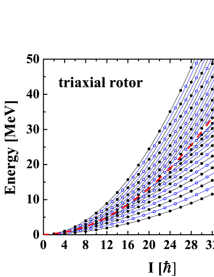
Figure 1: (Color online) Energy spectra as functions of spin $I$ for a triaxial rotor with $A_{1}=2A_{2}=6A_{3}=0.06~{}$MeV$/\hbar^{2}$ calculated by TRM. The full dots belong to the states with signature $\alpha=0$, while empty dots to signature $\alpha=1$. The approximate quantum number $n$ ($n=0,1,2,\cdots$) is introduced to label the energy states in accordance with the increasing order of their energies. Similar figure can be found in Ref. Frauendorf and Dönau (2014).

The obtained energy spectra can be divided into two different groups, which are distinguished by the manners of linking. One of them consists of the lines linking states with the same $n$ for $n$-small bands. With increasing spin, the energy spacing between neighboring lines become more and more equivalent. This is the classical wobbling regime, which corresponds to the wobbling motion around the axis with the largest MOI (i.e., 3-axis). The other one consists of the lines linking states with the same $I-n$ for $n$-large bands, which corresponds to the wobbling motion around the axis with the smallest MOI (i.e., 1-axis). Between them, it is the separatrix region. It has the energy of the unstable uniform rotation about the axis with the intermediate MOI.

To examine the accuracy of HA (13) and HP (II.2) formulas, the energy spectra and wobbling energies as functions of spin for the four lowest wobbling bands obtained by them are in comparison with the exact solutions by TRM and shown in Fig. 2. The wobbling energies, defined as the energy differences between the excited states and yrast state, are extracted from the obtained energy spectra and for a given spin $I$, are calculated as

$$E_{\textrm{wob}}=E(n,I)-E(0,I)$$ (22)

for even $I$, and

$$E_{\textrm{wob}}=E(n,I)-\frac{1}{2}[E(0,I-1)+E(0,I+1)]$$ (23)

for odd $I$.

It can be seen that the wobbling energies obtained by the three methods all increase with the spin. This phenomenon can be microscopically understood from the fact that the stiffness of the collective potential increases with spin Chen et al. (2014). Both the HA and HP methods can reproduce the TRM results for both energy spectra and wobbling energies over the whole spin range for small $n$ wobbling bands. However, with the increasing of $n$, the HA gradually deviates from the TRM results. For example, the HA results are larger than the TRM results about 150 keV for $n=2$ wobbling band and about 350 keV for $n=3$ wobbling band. This indicates that the wobbling motion is no longer with good harmonic vibrator character if $n$ becomes too large and the anharmonicity of wobbling motions begins to play an important role Jensen et al. (2002a); Oi and Fletcher (2005); Oi (2006). The occurrence of anharmonicity can be described by taking into account the higher order terms in the expansion of angular momenta. This statement is supported by the fact that HP formula reproduces the exact solutions perfectly. The energy differences between HP and TRM results are less than 30 keV even for $n=3$ wobbling band.

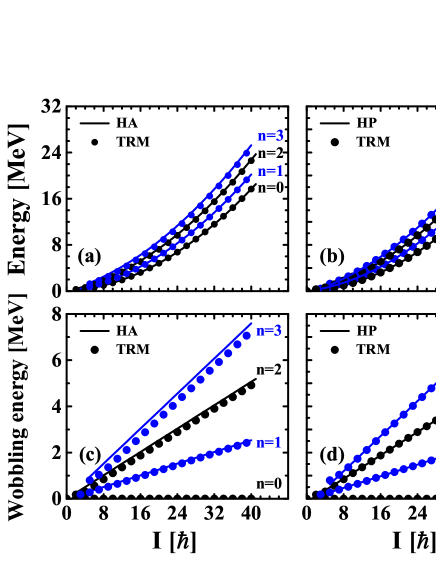
Figure 2: (Color online) The energy spectra and wobbling energies for the four lowest wobbling bands calculated by TRM are compared with those by HA (a, c) and HP (b, d) formulas.

To investigate the effects of the high order terms quantitatively, the energy differences obtained by the HA and HP methods are calculated

$$E_{\textrm{HA}}(n,I)-E_{\textrm{HP}}(n,I)$$

$$\quad=\frac{\alpha}{2}n^{2}-\Big{(}\frac{1}{2}\sqrt{\alpha^{2}-\beta^{2}}-\frac{\alpha}{2}\Big{)}(n+\frac{1}{2}).$$ (24)

It depends on wobbling phonon number $n$ while is independent of spin, i.e., the roles played by the next-to-leading term are different for different $n$ while are the same for different spin. It is obvious that with the increasing of $n$, the energy difference between HP and HA becomes larger, which indicates that the high order terms become more important and derive the wobbling motion deviates from harmonic vibrator behavior.

IV.2 Quadrupole transition probability

In Fig. 3, the intraband and interband $B(E2)$ values for $n=0$, $n=1$, and $n=2$ bands calculated by TRM in comparison with those by HA formula Bohr and Mottelson (1975) are shown. For the intraband $B(E2)$ values, the HA results given by Eq. (16) are constants, which are independent of spin $I$ and wobbling phonon number $n$. However, as shown in Fig. 3, the TRM results depend on not only spin but also wobbling phonon number. For each wobbling band $n$, the intraband $B(E2)$ values gradually increase with increasing spin and finally come close to the HA results at very high spin. For a given spin, with the increasing of $n$, the corresponding $B(E2)$ values decrease. Therefore, one can conclude that the HA formula is a good approximation only at very high spin and small $n$. This is expected since the approximation for vector addition coefficients in $E2$ matrix elements, which is valid only at very high spin, has been adopted when deriving the HA formula Bohr and Mottelson (1975).

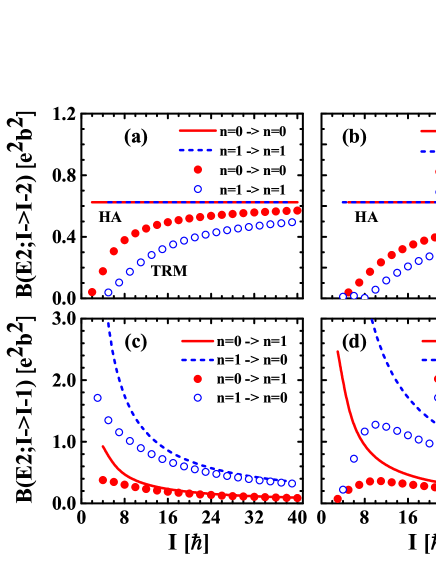
Figure 3: (Color online) The intraband and interband $B(E2)$ values for $n=0$, $1$ (a, c) and $n=1$, $2$ (b, d) bands calculated by TRM in comparison with those by HA formula Bohr and Mottelson (1975).

For interband $B(E2)$ values, the HA results exhibit decreasing trend with respect to spin for given $n$ and increasing trend with respect to $n$ for given spin, which are determined by the factor $n/I$ in the HA formulas (II.2) and (II.2). It can be further seen that the $B(E2;n,I\rightarrow n+1,I-1)$ values are smaller than the $B(E2;n+1,I\rightarrow n,I-1)$ values over the whole spin region since the bracketed terms in the Eq. (II.2) are smaller than the bracketed terms in the Eq. (II.2). For TRM results, the decreasing trends with respect to spin can also be found at high spin region. While at low spin region, contrary to the HA results, the increasing trend is shown for the interband transition between $n=1$ and $n=2$ bands. For example, the $B(E2;2,I\rightarrow 1,I-1)$ values increase rapidly with spin at $I\leq 10\hbar$.

It can be also seen that the HA results in general overestimate the TRM results. In particular, this overestimation becomes larger with the increasing of wobbling phonon number $n$. For a given $n$, the TRM results gradually come close to the HA results as spin increases. Therefore, similar to the case of intraband transition probabilities, the interband transition probabilities obtained by HA formula are good approximations for those by TRM only at high spin region and small $n$.

Comparing the interband transition with the intrband transition, it is seen that the strength of interband $B(E2;n,I\rightarrow n\pm 1,I-1)$ is smaller than that for the intraband $B(E2;n,I\rightarrow n,I-2)$ without changing the wobbling phonon number $n$ at high spin region, by a factor of order $\displaystyle\frac{n}{I}$, which represents the square of the amplitude of the wobbling motion Bohr and Mottelson (1975). This is the expected features of the wobbling bands, which corresponds to a sequence of one-dimensional rotational trajectories with strong $E2$ transition along the trajectories and much weaker transitions connecting the different trajectories Bohr and Mottelson (1975).

IV.3 Angular momentum

To understand the wobbling geometry picture, it is necessary to investigate the evolutions picture of angular momentum components with respect to spin $I$ and wobbling phonon number $n$. In Fig. 4, the angular momentum components $I_{k}$ as functions of spin for $n=0$-$5$ bands calculated by TRM are shown. For $n=0$ band, all of the three components of the angular momentum $I_{k}$ of the triaxial rotor gradually increase with spin increases. However, the roles played by them are quite different. The angular momentum favors aligning along the 3-axis with the largest MOI to obtain the lowest energy. The value of $I_{3}$ is nearly equal to $I$. The contributions from the other two axes to the total angular momentum are thus very small due to the conservation of the angular momentum

$$I_{1}^{2}+I_{2}^{2}+I_{3}^{2}=J^{2}=I(I+1).$$ (25)

It is worth pointing out that the angular momentum along the 3-axis and the other two axes (1-, 2-axis) respectively contribute the rotational energy and the zero energy of the wobbling motion for the wobbling energy spectra.

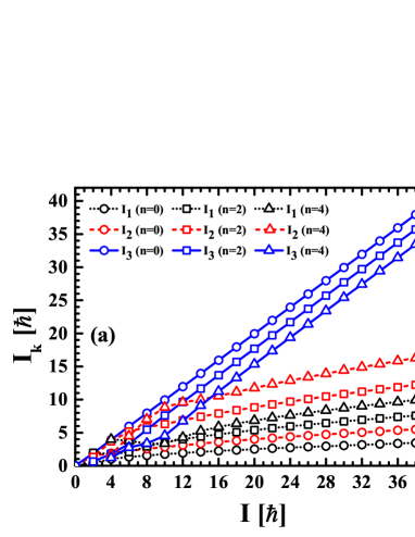
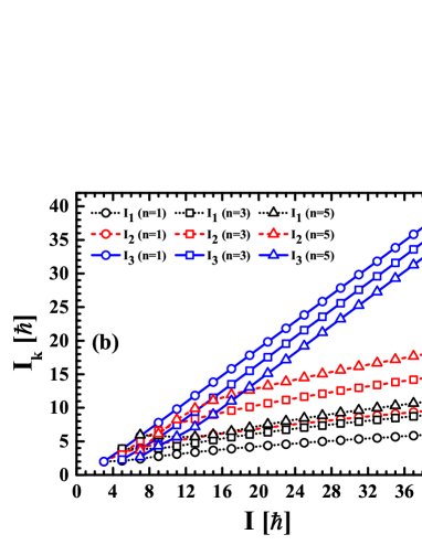
Figure 4: (Color online) The root mean square components along the 1, 2, and 3 axis of the total nucleus $I_{k}=\sqrt{\langle\hat{I}_{k}^{2}\rangle}$ calculated as functions of spin $I$ by TRM for (a) even $n$ wobbling bands ($n=0$, $2$, $4$) and (b) odd $n$ wobbling bands ($n=1$, $3$, $5$).

With the increasing of the wobbling phonon number $n$, the angular momentum shows a tendency to gradually deviate from the 3-axis. The value of $I_{3}$ is nearly equal to $I-n$ at large spin region. Meanwhile, the values of the 1- and 2- components of the angular momentum become larger and larger, which indicates that the wobbling motion plays a more and more important role.

It should be noted that when the wobbling phonon number $n$ is larger than 2, the three components of the angular momentum will present a strong competitive behavior. There exhibits a clear picture that with the increasing of spin the maximal component of the angular momentum changes from $I_{1}$ to $I_{2}$ and finally to $I_{3}$. Here, the evolution of the angular momentum with spin for $n=4$ band will be taken as an example to illustrate this picture. At spin $I=4\hbar$, the $n=4$ state is the largest energy state as shown in Fig. 1 and the angular momentum mainly aligns along the 1-axis, which corresponds to the wobbling motion along the axis with the smallest MOI. At spin region $6\leq I\leq 14\hbar$, the angular momentum turns to mainly align along the 2-axis with intermediate MOI. It can be seen from Fig. 1 that these states lie around the separatrix region. When spin $I>16\hbar$, the angular momentum finally mainly aligns along the 3-axis, which corresponds to the wobbling motion along the axis with the largest MOI. As shown in Fig. 1, these states are beneath the separatrix line and become further away from it as spin increases.

It has been emphasized that there exists complex competitions among three components of angular momenta with spin $I$ in the same $n$ wobbling bands. It is also interesting to investigate the evolution picture with respect to the wobbling phonon number for a given spin $I$. Therefore, in Fig. 5, the root mean square components along the 1, 2, and 3 axis of the total angular momentum $I_{k}$ calculated by TRM as functions of wobbling phonon number $n$ are shown respectively for $I=10\hbar$ (Fig. 5(a)) and $I=30\hbar$ (Fig. 5(b)).

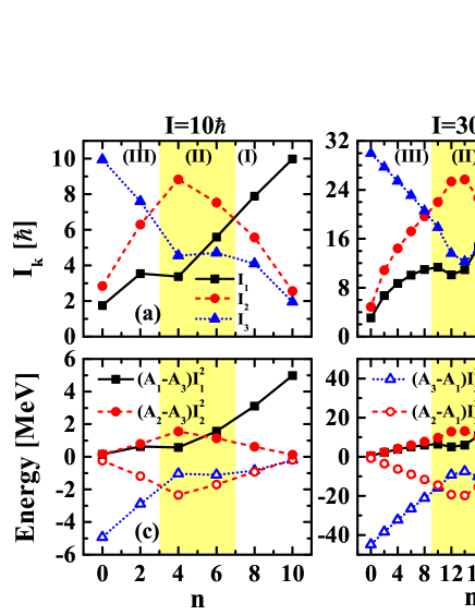
Figure 5: (Color online) The root mean square components along the 1, 2, and 3 axis of the total angular momentum $I_{k}=\sqrt{\langle\hat{I}_{k}^{2}\rangle}$ calculated by TRM and their corresponding contributions to the “kinetic” and “potential” terms of wobbling energy as functions of wobbling phonon number $n$ for $I=10\hbar$ (a, c) and $I=30\hbar$ (b, d).

For $I=10\hbar$, in general, the $I_{3}$ decreases while the $I_{1}$ increases as wobbling phonon number $n$ increases, which indicates that the angular momentum generally has a tendency to move away from 3-axis at small $n$ and to 1-axis at large $n$. However, $I_{3}$ shows a slightly increasing behavior when $n$ increases from 4 to 6. The angular momentum of $n=6$ state is closer to 3-axis than that of for $n=4$ state although the difference between them is small. This indicates that the angular momentum does not always steadily deviate from the 3-axis with increasing of $n$. It is further noted that $I_{1}$ also exhibits an abnormal behavior. When $n$ increases from 2 to 4, it decreases about $0.2\hbar$. Thereafter, it increases linearly with the increasing of $n$. Differing from the behaviors of $I_{1}$ and $I_{3}$, $I_{2}$ increases first at $n\leq 4$ and then decreases. Therefore, the strong competition among the three components of angular momentum is clearly presented. When $n=0$ and $2$, the $I_{3}$ is largest and $I_{2}>I_{1}$. This region is labeled as (III) in the figure. While when $n=4$ and $6$, $I_{2}$ becomes the largest component and $I_{1}$ and $I_{3}$ compete with each other. This region is labeled as (II). Finally, when $n$ increases to $8$ and $10$, $I_{1}$ begins to play the main role while $I_{3}$ turns to be the smallest. Correspondingly, this region is labeled as (I). For $I=30\hbar$, the evolution behaviors of three components of angular momentum are very similar to those for $I=10\hbar$. The abnormal behaviors exhibited by $I_{3}$ and $I_{1}$ happen at $n=14,16$ and $n=10,12$. For $I_{2}$, it reaches to maximal value at $n=14$. With increasing of $n$, the three components of angular momentum present a strong competitive behavior as well. Similar to the case of $I=10\hbar$, (III), (II), and (I) are labeled according to the maximal components of the angular momentum.

It can be thus concluded that with the increasing of the wobbling phonon number $n$ for a certain spin $I$, the simple triaxial rotor undergoes three different kinds of regions, as labeled (III), (II), and (I) regions in Fig. 5. In the region (III), $I_{3}$ is the largest, corresponding to the wobbling motion around the 3-axis with the largest MOI. This is further supported by the nearly equivalent contributions of “kinetic” term $(A_{2}-A_{3})I_{2}^{2}$ and “potential” term $(A_{1}-A_{3})I_{1}^{2}$ in this region, as shown in the Figs. 5(c) and (d). In addition, in this region, $I_{3}$ is approximately linear to $n$ with $I_{3}\approx I-n$. In the region (I), however, $I_{1}$ is the largest, which corresponds to the wobbling motion around the 1-axis with the smallest MOI. Similarly, this is also supported by the equivalent contributions of “kinetic” term $(A_{3}-A_{1})I_{3}^{2}$ and “potential” term $(A_{2}-A_{1})I_{2}^{2}$ in this region, as shown in the Figs. 5(c) and (d). Similar to $I_{3}$, $I_{1}$ is also approximately linear to $n$ with $I_{1}\approx n$ for even spin and $I_{1}\approx n+1$ for odd spin. In the transitional region (II), which corresponds to the separatrix region in Fig. 1, the $I_{1}$, $I_{2}$ and $I_{3}$ exhibit a completely different behavior from those shown in other two regions and fierce competitions among the three components of angular momentum is clearly shown. The fierce competitions might be associated with the phenomenon, as shown in Fig. 1, that the energy in this region increases slowly compared with those in other two regions as $n$ increases. In addition, although the $I_{2}$ is largest, there is not wobbling motion around 2-axis with the intermediate MOI since the “kinetic” term $(A_{1}-A_{2})I_{1}^{2}$ is positive ($A_{1}>A_{2}$) while the “potential” term $(A_{3}-A_{2})I_{3}^{2}$ negative ($A_{3}<A_{2}$). This conclusion is consistent with that obtained by tops-on-top model Sugawara-Tanabe et al. (2014).

In order to further clear draw the angular momentum evolution pictures, in Fig. 6, the orientation of the total angular momentum, depicted by the polar angle $\theta$ (11) and azimuth angle $\varphi$ (11), as a function of wobbling phonon number $n$ for $I=10$, $20$, $30$ and $40\hbar$ are illustrated.

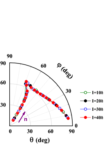
Figure 6: (Color online) The calculated orientation of the total angular momentum, depicted by the polar angle $\theta$ and azimuth angle $\varphi$, as a function of wobbling phonon number $n$ for $I=10$, $20$, $30$ and $40\hbar$. The $\theta$ and $\varphi$ are shown in a polar coordinate system, in which $\theta$ is the radial coordinate while $\varphi$ the angular coordinate. The arrow indicates the increasing direction of wobbling phonon number.

It is clearly seen that the series of points with the wobbling phonon number $n$ for all spin $I$ lies on the same line, which indicates that no matter what spin $I$ is, the orientations of angular momentum vectors are along the same evolution track with the increasing of $n$. When $n$ is small, the $\varphi$ is almost invariable while the $\theta$ increases as $n$ increases, which suggests that the angular momentum vector lies almost in the same plane $\varphi\approx 60^{\circ}$ but gradually deviates from the 3-axis as $n$ increases. The reason of angular momentum being in the plane $\varphi\approx 60^{\circ}$ can be understood according to the “kinetic” and “potential” terms in the TRM Hamiltonian as shown in the Figs. 5(c) and (d). Since the “kinetic” term $(A_{2}-A_{3})I_{2}^{2}$ and “potential” term $(A_{1}-A_{3})I_{1}^{2}$ are almost equivalent for small $n$, it indicates that $\varphi=\tan^{-1}\Big{(}\displaystyle\frac{I_{2}}{I_{1}}\Big{)}$ approximates as $\tan^{-1}\sqrt{\displaystyle\frac{A_{2}-A_{3}}{A_{1}-A_{3}}}$. Thus $\varphi$ is independent on $\theta$ but determined by the three MOIs at small $n$. According to this formula, one can obtain $\varphi\approx 60^{\circ}$ in the present discussed system. It is noted that these energy states correspond to the wobbling motion along the 3-axis and mainly lie in the region (III) as shown in Fig. 5. As $n$ increases, both $\theta$ and $\varphi$ increase, which suggests that the angular momentum not only continues deviating from the 3-axis, but also starts moving to the 2-axis. However, the increasing trend of $\varphi$ will not be incessant but will interrupt up to a critical point. This critical point corresponds to the maximal values of $I_{2}$, as shown in the Fig. 5(a) and (b). After that, the $\varphi$, together with $\theta$, begins to decrease. It indicates that the angular momentum moves to the 1-axis, and also moves slightly to the 3-axis in the meantime. The points around the critical point correspond to the transition region (II) shown in Fig. 5. After crossing this regions, $\varphi$ decreases while $\theta$ increases with the increasing of $n$, moving to region (I) shown in Fig. 5. Similar to the cases of small $n$, according to Figs. 5(c) and (d), in this region it has $\displaystyle\frac{I_{3}}{I_{2}}=\sqrt{\frac{A_{3}-A_{1}}{A_{2}-A_{1}}}$, which implies that the angular momentum vectors for large $n$ lie also in the same plane that is perpendicular to the 2-3 plane.

According to the above discussions, the evolution track of angular momenta with respect to the wobbling phonon number presented in Fig. 6 is determined only by the three MOIs of the triaxial rotor. As already pointed out above, the evolution track is unique and irrespective of what spin is. From this point of view, this evolution track may be regarded as a characteristic feature for a rotating triaxial rotor. Just along this evolution track, the triaxial rotor changes its rotation along the axis with the largest MOI to the axis with the smallest MOI.

IV.4 $K$-distribution

In the above, the angular momentum geometry of wobbling motion for the triaxial rotor are investigated via the expectation values of the three components of the angular momentum. It is interesting to further investigate the angular momentum geometry pictures from a microscopic perspective by the obtained wave functions. In the TRM, the wave functions can be directly reflected by the so called $K$-distributions, i.e., the probability distributions of projection of total angular momentum on the 1-, 2- and 3- axis. In the literatures, by the PRM, such $K$-distributions have been extensively applied to study the angular momentum geometry of the nuclear chiral modes in triaxial nuclei Qi et al. (2009a, b); Chen et al. (2010); Qi et al. (2011).

In the following, the $K$-distributions for the $n=0$, $2$, $4$ states with $I=10$ and $30\hbar$ and $n=1$, $3$, $5$ states with $I=9$ and $29\hbar$, shown in Fig. 7, are taken as examples to microscopically understand the angular momenta geometry.

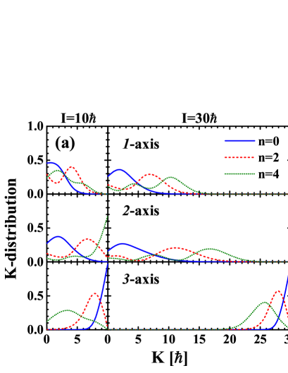
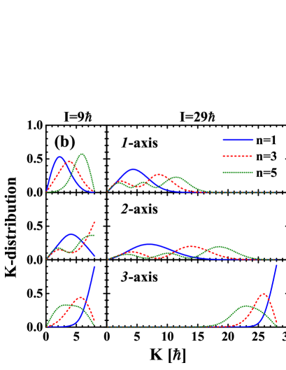
Figure 7: (Color online) The probability distributions for projection of total angular momentum on the 1-, 2- and 3- axis in TRM for (a) $n=0$, $2$, $4$ states with $I=10$ and $30\hbar$ and (b) $n=1$, $3$, $5$ states with $I=9$ and $29\hbar$.

It can be seen that for $n=0$ states, the maximal probability for the 3-axis appears at $K_{3}=I$ for both $I=10$ and $30\hbar$, while the probabilities for the other $K_{3}$ values almost vanish. This is expected since the angular momentum mainly along, as shown in Fig. 5, 3-axis. The probability distributions with respect to the 2- and 1-axis have peaks near $K_{2}=2\hbar$ and $K_{1}=2\hbar$ for both $I=10$ and $30\hbar$. The reason why these peaks do not appear at $K_{2}=0$ and $K_{1}=0$ is attributed to the nature of three dimensional rotation of the triaxial rotor, where three angular momentum components $I_{k}$ all have contributions to the total spin. As the MOI of 2-axis is larger than that of 1-axis, the angular momentum is closer to 2-3 plane than 1-3 plane. Thus the tunneling of angular momentum with respect to the 2-3 plane is easier than to 1-3 plane. This phenomenon can be reflected by the probability for $K_{1}=0$ is larger than that for $K_{2}=0$.

As $n$ increases, for large spin, e.g., $I=29$ and $30\hbar$, the peak of the probability on 3-axis moves away from the $K=I$ to $K=I-n$ corresponding to a deviation from the 3-axis, which suggests that the distributions from $I_{1}$ and $I_{2}$ become more important. Meanwhile, for $K_{1}$ and $K_{2}$, more peaks appear and it is expected that the number of peaks is $n+1$ if the $K$ distributions are plotted also for negative $K$ values. It is noted that for the even $n$ and odd $n$ states, the probabilities on the 1- and 2- axis are respective nonzero and zero at $K=0$, which indicates that their corresponding wave functions are symmetric and antisymmetric in the projections on the 1- and 2- axis. We should bear in mind that all the presented states for large spin lie in the region (III), where the wobbling motions happen along the axis with largest MOI. Once the states lying in the other two regions are involved, the $K$ distributions would exhibit a different behavior. This can be seen for small spin when $n$ is not too large, e.g., $n=4$ state with $I=10\hbar$, which lies in the region (II). Therefore, further investigation for the evolutions of $K$ distribution with respect to the wobbling phonon number $n$ is necessary.

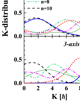
Figure 8: (Color online) Same as Fig. 7, but for the $n=0$-$10$ states with $I=10\hbar$.

In Fig. 8, the $K$ distributions for the $n=0$-$10$ states are shown. For $n=4$, the probability for $K_{2}=I=10\hbar$ is much larger than that for other $K_{2}$. Comparing with the region (II) in Fig. 5, this corresponds to the situation that $I_{2}$ is the largest angular momentum components and the angular momentum mainly aligns along the 2-axis. In this case, the probability distributions with respect to the 1- and 3-axis have peaks near $K_{1}=2\hbar$ and $K_{3}=4\hbar$. As $n$ increases, the peak of the probability on 1-axis gradually moves towards to $K_{1}=I$ and the peaks for each $n$ state appear nearly at $K_{1}=n$, which indicates a tendency of the angular momentum moving to the 1-axis. This evolution picture is consistent with the evolution picture of angular momentum shown in Fig. 5.

It is interesting to note that the $K$ distribution on the 1-axis and 3-axis for the $n=8$ and $n=10$ states are respectively similar to those distributions on the 3-axis and 1-axis for the $n=2$ and $n=0$ states. Moreover, the $K$ distribution on the 2-axis for $n=0$ and $n=10$ states as well as $n=2$ and $n=8$ states are also very similar. These similar behaviors are justified since the wobbling motions happen both along 1- and 3- axis. These similarity between the pictures for wobbling motion around 1-axis and 3-axis are consistent with the pictures of components of angular momentum shown in Fig. 5.

V Summary

In summary, a simple triaxial rotor is taken as an example to illustrate the picture of wobbling motion by exactly solving the TRM Hamiltonian. The obtained energy spectra and reduced quadrupole transition probabilities are compared to those approximate analytic solutions by HA Bohr and Mottelson (1975) and HP Tanabe and Sugawara-Tanabe (1971, 2006, 2008) methods to evaluate the accuracy of the analytic methods. It is found that only the low lying wobbling bands can be well described by the analytic HA solutions. By taking the higher order terms into account, the HP method improves the HA descriptions for the energy spectra.

The evolution of angular momentum geometry with respect to the spin and the wobbling phonon number are investigated. It is confirmed that with the increasing of wobbling phonon number, the triaxial rotor changes its rotation along the axis with the largest MOI to the axis with the smallest MOI. There is a competitive process among three angular momentum components in the separatrix region in which the angular momentum mainly aligns along the axis with intermediate MOI. Nevertheless, a specific track that can be used to depict the motion of a triaxial rotating nuclei at any spin is found along the evolutionary process. This evolutionary track may be regarded as a fingerprint of the triaxial rotor. The $K$-distribution further corroborates the evolution picture of the angular momentum.

For a perspective, it is interesting to investigate the angular momentum geometry of wobbling motion for odd-$A$ nuclei, in particular the angular momentum geometry of longitudinal and transverse wobblers Frauendorf and Dönau (2014).

References

- Bohr and Mottelson (1975) A. Bohr and B. R. Mottelson, Nuclear structure, vol. II (Benjamin, New York, 1975).
- Frauendorf and Meng (1997) S. Frauendorf and J. Meng, Nucl. Phys. A 617, 131 (1997).
- Frauendorf (2001) S. Frauendorf, Rev. Mod. Phys. 73, 463 (2001).
- Meng and Zhang (2010) J. Meng and S. Q. Zhang, J. Phys. G: Nucl. Part. Phys. 37, 064025 (2010).
- Ødegård et al. (2001) S. W. Ødegård, G. B. Hagemann, D. R. Jensen, M. Bergström, B. Herskind, G. Sletten, S. Törmänen, J. N. Wilson, P. O. Tjøm, I. Hamamoto, et al., Phys. Rev. Lett. 86, 5866 (2001).
- Jensen et al. (2002a) D. R. Jensen, G. B. Hagemann, I. Hamamoto, S. W. Ødegård, B. Herskind, G. Sletten, J. N. Wilson, K. Spohr, H. Hübel, P. Bringel, et al., Phys. Rev. Lett. 89, 142503 (2002a).
- Jensen et al. (2002b) D. R. Jensen, G. B. Hagemann, I. Hamamoto, S. W. Ødegård, M. Bergstrom, B. Herskind, G. Sletten, S. Tormanen, J. N. Wilson, P. O. Tjom, et al., Nucl. Phys. A 703, 3 (2002b).
- Schönwaßer et al. (2003) G. Schönwaßer, H. Hübel, G. B. Hagemann, P. Bednarczyk, G. Benzoni, A. Bracco, P. Bringel, R. Chapman, D. Curien, J. Domscheit, et al., Phys. Lett. B 552, 9 (2003).
- Amro et al. (2003) H. Amro, W. C. Ma, G. B. Hagemann, R. M. Diamond, J. Domscheit, P. Fallon, A. Gorgen, B. Herskind, H. Hubel, D. R. Jensen, et al., Phys. Lett. B 553, 197 (2003).
- Hagemann (2004) G. B. Hagemann, Eur. Phys. J. A 20, 183 (2004).
- Bringel et al. (2005) P. Bringel, G. Hagemann, H. Hübel, A. Al-khatib, P. Bednarczyk, A. Bürger, D. Curien, G. Gangopadhyay, B. Herskind, D. Jensen, et al., Eur. Phys. J. A 24, 167 (2005).
- Hartley et al. (2009) D. J. Hartley, R. V. F. Janssens, L. L. Riedinger, M. A. Riley, A. Aguilar, M. P. Carpenter, C. J. Chiara, P. Chowdhury, I. G. Darby, U. Garg, et al., Phys. Rev. C 80, 041304 (2009).
- Zhu et al. (2009) S. J. Zhu, Y. X. Luo, J. H. Hamilton, A. V. Ramayya, X. L. Che, Z. Jiang, J. K. Hwang, J. L. Wood, M. A. Stoyer, R. Donangelo, et al., Int. J. Mod. Phys. E 18, 1717 (2009).
- Hamamoto (2002) I. Hamamoto, Phys. Rev. C 65, 044305 (2002).
- Hamamoto and Mottelson (2003) I. Hamamoto and B. R. Mottelson, Phys. Rev. C 68, 034312 (2003).
- Frauendorf and Dönau (2014) S. Frauendorf and F. Dönau, Phys. Rev. C 89, 014322 (2014).
- Shimizu and Matsuzaki (1995) Y. R. Shimizu and M. Matsuzaki, Nucl. Phys. A 588, 559 (1995).
- Matsuzaki et al. (2002) M. Matsuzaki, Y. R. Shimizu, and K. Matsuyanagi, Phys. Rev. C 65, 041303 (2002).
- Matsuzaki et al. (2003) M. Matsuzaki, Y. R. Shimizu, and K. Matsuyanagi, Eur. Phys. J. A 20, 189 (2003).
- Matsuzaki et al. (2004) M. Matsuzaki, Y. R. Shimizu, and K. Matsuyanagi, Phys. Rev. C 69, 034325 (2004).
- Matsuzaki and Ohtsubo (2004) M. Matsuzaki and S. Ohtsubo, Phys. Rev. C 69, 064317 (2004).
- Shimizu et al. (2005) Y. R. Shimizu, M. Matsuzaki, and K. Matsuyanagi, Phys. Rev. C 72, 014306 (2005).
- Shimizu et al. (2008) Y. R. Shimizu, T. Shoji, and M. Matsuzaki, Phys. Rev. C 77, 024319 (2008).
- Shoji and Shimizu (2009) T. Shoji and Y. R. Shimizu, Progr. Theor. Phys. 121, 319 (2009).
- Oi et al. (2000) M. Oi, A. Ansari, T. Horibata, and N. Onishi, Phys. Lett. B 480, 53 (2000).
- Chen et al. (2014) Q. B. Chen, S. Q. Zhang, P. W. Zhao, and J. Meng, Phys. Rev. C 90, 044306 (2014).
- Tanabe and Sugawara-Tanabe (1971) K. Tanabe and K. Sugawara-Tanabe, Phys. Lett. B 34, 575 (1971).
- Tanabe and Sugawara-Tanabe (2006) K. Tanabe and K. Sugawara-Tanabe, Phys. Rev. C 73, 034305 (2006).
- Tanabe and Sugawara-Tanabe (2008) K. Tanabe and K. Sugawara-Tanabe, Phys. Rev. C 77, 064318 (2008).
- Davydov and Filippov (1958) A. Davydov and G. Filippov, Nuclear Physics 8, 237 (1958).
- Zeng (2007) J. Y. Zeng, Quantume mechanics, vol. II (Science Press, Beijing, 2007), in Chinese.
- Holstein and Primakoff (1940) T. Holstein and H. Primakoff, Phys. Rev. 58, 1098 (1940).
- Oi and Fletcher (2005) M. Oi and J. Fletcher, J. Phys. G 31, S1753 (2005).
- Oi (2006) M. Oi, Phys. Lett. B 634, 30 (2006).
- Sugawara-Tanabe et al. (2014) K. Sugawara-Tanabe, K. Tanabe, and N. Yoshinaga, Prog. Theor. Exp. Phys. 2014, 063D01 (2014).
- Qi et al. (2009a) B. Qi, S. Q. Zhang, J. Meng, S. Y. Wang, and S. Frauendorf, Phys. Lett. B 675, 175 (2009a).
- Qi et al. (2009b) B. Qi, S. Q. Zhang, S. Y. Wang, J. M. Yao, and J. Meng, Phys. Rev. C 79, 041302(R) (2009b).
- Chen et al. (2010) Q. B. Chen, J. M. Yao, S. Q. Zhang, and B. Qi, Phys. Rev. C 82, 067302 (2010).
- Qi et al. (2011) B. Qi, S. Q. Zhang, S. Y. Wang, J. Meng, and T. Koike, Phys. Rev. C 83, 034303 (2011).