Higher dimensional Frobenius problem: Maximal saturated cone, growth function and rigidity

Abstract.

We consider $m$ integral vectors $X_{1},\dots,X_{m}\in\mathbb{Z}^{s}$ located in a half-space of $\mathbb{R}^{s}$ ($m\geq s\geq 1$) and study the structure of the additive semi-group $X_{1}\mathbb{N}+\dots+X_{m}\mathbb{N}$. We introduce and study maximal saturated cone and directional growth function which describe some aspects of the structure of the semi-group. When the vectors $X_{1},\cdots,X_{m}$ are located in a fixed hyperplane, we obtain an explicit formula for the directional growth function and we show that this function completely characterizes the defining data $(X_{1},\cdots,X_{m})$ of the semi-group. The last result will be applied to the study of Lipschitz equivalence of Cantor sets (see [13]).

1. Introduction

We consider $m$ integral vectors $X_{1},\dots,X_{m}$ in the lattice $\mathbb{Z}^{s}$ ($m\geq 2$, $s\geq 1$) which are assumed to be in a half-space. That is to say, there is a vector ${\boldsymbol{\alpha}}\in{\mathbb{R}}^{s}$ such that $\langle X_{j},{\boldsymbol{\alpha}}\rangle>0$ for all $j=1,\dots,m$ where $\langle\cdot,\cdot\rangle$ denotes the inner product on the Euclidean space $\mathbb{R}^{s}$. We also assume that $X_{1},\dots,X_{m}$ span the vector space $\mathbb{R}^{s}$. But $X_{j}$’s may not be distinct. Let

(1.1) $$\mathcal{J}=X_{1}\mathbb{N}+\dots+X_{m}\mathbb{N}$$

be the semi-group generated by $X_{1},\dots,X_{m}$ where $\mathbb{N}=\{0,1,2,\dots\}$ denotes the set of natural numbers. By higher dimensional Frobenius problem we mean the study of the structure of the semi-group $\mathcal{J}$ defined by (1.1). This will be our main concern in the present paper.

In the one-dimensional case (i.e. $s=1$), we are given $m$ relatively prime positive integers $a_{1},\cdots,a_{m}$ instead of $X_{1},\cdots,X_{m}$. Then

$${\mathcal{J}}=a_{1}\mathbb{N}+\dots+a_{m}\mathbb{N}$$

which is the set of all natural numbers representable as a non-negative integer combination of $a_{1},\cdots,a_{m}$. Sylvester [16] showed that there exists a minimum positive number $f(a_{1},\dots,a_{m})$, which is now called the Frobenius number, such that

$$f(a_{1},\dots,a_{m})+1+\mathbb{N}\subset{\mathcal{J}}.$$

The following so-called diophantine Frobenius Problem was raised by F. G. Frobenius (see [1]): find $f(a_{1},\dots,a_{m})$ the largest natural number that is not representable as a non-negative integer combination of $a_{1},\cdots,a_{m}$.

Sylvester’s result says that a translation of the set $\mathbb{N}$ is contained in $\mathcal{J}$. Thus the structure of $\mathcal{J}$ is rather well described by the Frobenius number. It turned out that the knowledge of $f(a_{1},\dots,a_{m})$ has been extremely useful to investigate many different problems. When $m=2$, it is well-known that

$$f(a_{1},a_{2})=a_{1}a_{2}-a_{1}-a_{2}.$$

For example, if $a_{1}=3$ and $a_{2}=5$, then

$${\mathcal{J}}=3\mathbb{N}+5\mathbb{N}=\{0,3,5,6,8,9,10,11,\dots\}$$

and $f(3,5)=7$. However, for $m\geq 3$, there is no closed form for $f(a_{1},\cdots,a_{m})$. It is proved that the Frobenius problem is NP-hard under Turing reductions. The book of Ramírez-Alfonsín [1] (2005) is a nice survey on the Frobenius problem.

Our study of higher dimensional Frobenius problem is motivated by the study of Lipschitz equivalence of Cantor sets. Lipschitz equivalence preserves many important properties of a self-similar set. A survey on Lipschitz equivalence of Cantor sets can be found in [12], see also [10]. In this area, a fundamental problem initially raised by Falconer and Marsh [5], which is now called the Falconer-Marsh problem, is as follows: Assume that two self-similar sets $E$ and $F$ are dust-like. How is the Lipschitz equivalence related to the contraction ratios of $E$ and $F$ ? Falconer and Marsh [5] established several basic techniques and results in 1992. But there is no progress until recent works of Rao, Ruan and Wang [11] (2012) and Xiong and Xi [17] (2013).

Xiong and Xi [17] studied the case when $E$ and $F$ have rank $1$ (i.e. contraction ratios are powers of a fixed number) and discovered that the problem is closely related to the class number of the field generated by the ratios.

Rao, Ruan and Wang [11] introduce a Lipschitz invariant described by a so-called matchable condition. They solved the problem when both $E$ and $F$ have full rank or both of them are two-branch self-similar sets. However, the matchable condition is hard to check in general. The present paper and the sequential paper [13] introduce new techniques to handle the matchable condition. We associate to each self-similar set a higher dimensional Frobenius problem. We find that this is closely related to the matchable condition. Thanks to this link, in [13], we solve the Falconer-Marsh problem in the case that the contraction ratios of the self-similar sets satisfy a coplanar condition.

In the following subsections we will describe in some detail our results obtained in the paper. Here is a resumé. Two aspects of the structure of the semi-group $\mathcal{J}$ defined by (1.1) will be first studied: one is the existence and finiteness of maximal saturated cones (Section 2) and the other is the growth function which describes how many ways a given vector $z$ in $\mathcal{J}$ can be represented by finite sums of terms from $\{X_{1},...,X_{m}\}$. We shall prove that it is a function which increases exponentially as $\|z\|$ tends to the infinity and that the increasing rate depends on the direction along which $\|z\|$ tends to the infinity (Section 3 and Section 4). Thus we obtain the so-called directional growth function. An explicit formula is obtained for the directional growth function when the vectors $X_{1},\cdots,X_{m}$ are located on a same hyperplane (Section 5). The last two sections are devoted to the rigidity. The rigidity means, if two growth functions are equal, then the corresponding semi-groups are equal. Furthermore, the sets of vectors defining the semi-groups are the same. These rigidity results are proved under the assumption that the defining vectors are coplanar.

In the following subsections, we state our results in some details.

1.1. Maximal saturated cone

Recall that $X_{1},\dots,X_{m}$ are $m$ given vectors in the lattice $\mathbb{Z}^{s}$ ($m\geq 2$, $s\geq 1$) such that $\langle X_{j},{\boldsymbol{\alpha}}\rangle>0$ for all $j=1,\dots,m$ and for some vector ${\boldsymbol{\alpha}}\in\mathbb{R}^{s}$. For simplicity we use ${X}$ to denote the set $\{X_{1},\dots,X_{m}\}$. Let

(1.2) $${\mathcal{L}}:={\mathcal{L}}_{X}:=X_{1}\mathbb{Z}+\cdots+X_{m}\mathbb{Z}$$

denote the lattice generated by $X_{1},\dots,X_{m}$. Let

(1.3) $${\mathbf{C}}_{X}:=X_{1}\mathbb{R}^{+}+\cdots+X_{m}\mathbb{R}^{+}$$

denote the convex cone generated by $X_{1},\dots,X_{m}$, where $\mathbb{R}^{+}$ is the set of non-negative real numbers. Clearly, the semi-group $\mathcal{J}$ is a subset of the lattice ${\mathcal{L}}$ so that

$$\forall g\in\mathcal{J},\quad(g+{\mathbf{C}}_{X})\cap{\mathcal{J}}\subset(g+{\mathbf{C}}_{X})\cap\mathcal{L}.$$

If $(g+{\mathbf{C}}_{X})\cap{\mathcal{J}}=(g+{\mathbf{C}}_{X})\cap\mathcal{L}$, the cone $g+{\mathbf{C}}_{X}$ is said to be saturated. That means, every lattice point in the cone $g+{\mathbf{C}}_{X}$ is in the semi-group. Moreover, a saturated cone is said to be maximal if it is not a subset of any other saturated cone. Then we define the Frobenius set to be

(1.4) $${\mathcal{F}}:=\{g\in\mathcal{J}:~{}g+{\mathbf{C}}_{X}\text{ is a maximal saturated cone}\}.$$

Let us look at the one-dimensional case considered above with $X_{j}=a_{j}$. The cone ${\mathbf{C}}_{X}$ is then equal to $\mathbb{R}^{+}$. The cone $g+\mathbb{R}^{+}$ is saturated if and only if $g>f(a_{1},\dots,a_{m})$. Therefore we have ${\mathcal{F}}=\{f(a_{1},\dots,a_{m})+1\}$, the singleton consisting of the smallest natural number such that all larger natural numbers are representable as a non-negative integer combination of $a_{1},\cdots,a_{m}$.

A natural question is “how many maximal saturated cones are there ?” Our answer is

Theorem 1.1.

The Frobenius set ${\mathcal{F}}$ is non-empty and finite.

Here is an example where the Frobenius set has two elements. Let $s=2$ and $X=\{(3,0),(1,2),(0,3)\}$. Then ${\mathbf{C}}_{X}=\mathbb{R}^{+}\times\mathbb{R}^{+}$ and

$$\mathcal{L}=\{(a,b)\in\mathbb{Z}^{2};~{}a+b\text{ is a multiple of }3\},$$

$$\mathcal{J}=\{(a,b)\in\mathbb{N}^{2};~{}a+b\text{ is a multiple of }3\text{ and }b\neq 1\}.$$

We find ${\mathcal{F}}=\{(1,2),(0,3)\}$. This is shown in Figure 1.

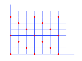
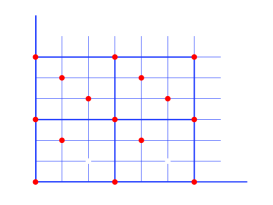
Figure 1. Example 1.3: $\mathcal{L}$ (left) and $\mathcal{J}$ (right).

1.2. Multiplicity of representations and directional growth function

For any vector $z$ in the semi-group $\mathcal{J}$, we are interested in the number of representations $z=X_{i_{1}}+\cdots+X_{i_{n}}$ where $n\geq 1$ and $i_{k}$’s are taken from $\{1,2,\cdots,m\}$. As we shall see, these numbers reflect some property of the structure of the semi-group.

Let $\Sigma_{m}^{*}:=\bigcup_{k=0}^{\infty}\{1,2,\dots,m\}^{k}$ be the set of words over the alphabet $\{1,2,\dots,m\}$, which can also be considered as a tree. For any word $\mathbf{i}=i_{1}\dots i_{n}\in\Sigma_{m}^{*},$ define

(1.5) $$\kappa(\mathbf{i})=X_{i_{1}}+\cdots+X_{i_{n}}.$$

We consider $\kappa:\Sigma_{m}^{*}\to\mathbb{Z}^{s}$ as the walk in $\mathbb{Z}^{s}$ guided by $X_{1},\dots,X_{m}$ along with the tree $\Sigma_{m}^{*}$. Elements in $\Sigma_{m}^{*}$ are also called pathes of the walk and $\kappa(\mathbf{i})$ is called the visited position following the path $\mathbf{i}$. A point $z\in\mathbb{Z}^{s}$ is said to be attainable if $z=\kappa(\mathbf{i})$ for some ${\mathbf{i}}\in\Sigma_{m}^{*}.$ Clearly the set of attainable positions is exactly the semi-group ${\mathcal{J}}$. A second question we ask is “How many times is an attainable position visited ?”

To partially answer this question, for $z\in\mathcal{J}$, we define the multiplicity of $z$ to be

(1.6) $${\mathbf{m}}(z):=\#\{\omega\in\Sigma_{m}^{*};\ \kappa(\omega)=z\}.$$

We extend the function ${\mathbf{m}}$ to the convex cone ${\mathbf{C}}_{X}$ as follows. For any point $x\in{\mathbf{C}}_{X}$ but not in ${\mathcal{J}}$, instead of setting ${\mathbf{m}}(x)=0$, we define its multiplicity to be the multiplicity of the point in $\mathcal{J}$ which is nearest to $x$. More precisely,

(1.7) $${\mathbf{m}}(x):=\min\{{\mathbf{m}}(z);\ z\in{\mathcal{J}}\text{ and }\|x-z\|=d(x,{\mathcal{J}})\},$$

where $\|\cdot\|$ denotes the Euclidean norm and $d(x,{\mathcal{J}}):=\min\{\|x-z\|;~{}z\in{\mathcal{J}}\}$.

In the one-dimensional case, the multiplicity ${\mathbf{m}}$ restricted on $\mathcal{J}$ satisfies the linear recurrent relation

$${\mathbf{m}}(n)=\sum_{j=1}^{m}{\mathbf{m}}(n-a_{j}).$$

Hence we can obtain an explicit formula for ${\mathbf{m}}(n)$. It is then easy to show that ${\mathbf{m}}(n)$ is of the same exponential order as $\beta^{n}$ where $\beta$ is the largest root of the equation

$$x^{a_{m}}-\sum_{j=1}^{m}x^{a_{m}-a_{j}}=0.$$

(See, for instance, [2]). But in the higher dimensional case, it is hard to obtain an explicit formula for the multiplicity. Nevertheless, we will prove the following exponential growth.

Theorem 1.2.

For any unit vector $\theta\in{\mathbf{C}}_{X}$, the following limit exists

(1.8) $$\gamma(\theta)=\underset{k\rightarrow\infty}{\lim}\frac{\log\mathbf{m}(k\theta)}{k}.$$

We call $\gamma$ the directional growth function of the semi-group $\mathcal{J}$. It describes the exponential increasing speed of the multiplicity along the direction $\theta$. We will first prove that the multiplicity function varies slowly in the sense that the quotient of $\mathbf{m}(z)$ and $\mathbf{m}(z^{\prime})$ is of polynomial order of $\|z\|$ if $z^{\prime}$ and $z$ have a bounded distance (Theorem 3.3). We will then prove that the sequence $(\log\mathbf{m}(k\theta))_{k\geq 1}$ is subadditive in some weak sense, which is sufficient to ensure the existence of the limit in (1.8), according to Lemma 4.1 which strengthens a classical result on sub-additive sequence.

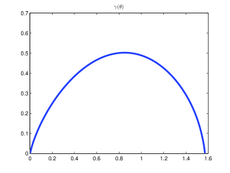
Figure 2. The function $\gamma(\theta)$ for $X=\{(3,0),(1,2),(0,3\}$.

1.3. Calculation of $\gamma(\theta)$ when $X_{1},\cdots,X_{m}$ are coplanar

In general, it is difficult to obtain an explicit formula of $\gamma(\theta)$. We will be confined to a formula under the condition that $X_{1},\cdots,X_{m}$ are coplanar.

We say that $X_{1},\dots,X_{m}$ are coplanar if they locate on a same hyper-plane, i.e. there exists a vector $\eta\in\mathbb{R}^{s}$ such that

(1.9) $$\langle\eta,X_{j}\rangle=1,\quad j=1,\dots,m.$$

To be more precise, we say $X_{1},\dots,X_{m}$ are $\eta$-coplanar. Let $p=(p_{1},\dots,p_{m})$ be a probability vector. The entropy of $p$ is defined as

$$h(p)=-\sum_{j=1}^{m}p_{j}\log p_{j}.$$

Theorem 1.3.

Suppose that $X_{1},\dots,X_{m}$ are $\eta$-coplanar. For any unit vector $\theta$ in the cone ${\mathbf{C}}_{X}$, we have

(1.10) $$\gamma(\theta)={\langle\theta,\eta\rangle}\sup\left\{h(p);~{}p_{1}X_{1}+\cdots+p_{m}X_{m}=\frac{\theta}{\langle\theta,\eta\rangle}\right\}.$$

There is another expression involving the following function $\log\sum_{j=1}^{m}e^{\langle t,X_{j}\rangle},$ $t\in\mathbb{R}^{s},$ which corresponds to the pressure function in the statistic physics (Theorem 6.2). The above formula (1.10) resembles the conditional variation principle in the analysis of multifractal analysis (see [7], see also [6], [8]). Actually, the proof of Theorem 1.3 uses the idea of large deviation. If $X_{1},\dots,X_{m}$ are linearly independent, then the choice of $p$ is unique and we can easily compute $\gamma(\theta)$.

Here is an example. Let $s=2$ and $X=\{(1,0),(0,1)\}$. Then ${\mathbf{C}}_{X}=(\mathbb{R}^{+})^{2},\ {\mathcal{J}}=\mathbb{N}^{2},$ $\mathcal{L}=\mathbb{Z}^{2}$ and $\eta=(1,1)$. Clearly $\mathbf{m}(a,b)=\frac{(a+b)!}{a!b!}.$ For $\theta=(\theta_{1},\theta_{2})$ with $\theta_{1}^{2}+\theta_{2}^{2}=1$ and $\theta_{1},\theta_{2}\geq 0$. Let $p_{1}=\theta_{1}/(\theta_{1}+\theta_{2})$, $p_{2}=\theta_{2}/(\theta_{1}+\theta_{2})$. This vector $(p_{1},p_{2})$ is the unique probability satisfying $p_{1}X_{1}+p_{2}X_{2}=\theta/\langle\eta,\theta\rangle$. Then

$$\gamma(\theta)=(\theta_{1}+\theta_{2})h(p_{1},p_{2}).$$

The unit vector $(\theta_{1},\theta_{2})$ can be described by the angle $\alpha\in[0,\pi/2]$ such that $\theta_{1}=\cos\alpha$. Then

$$\gamma(\alpha)=-\cos\alpha\log\frac{\cos\alpha}{\cos\alpha+\sin\alpha}-\sin\alpha\log\frac{\sin\alpha}{\cos\alpha+\sin\alpha}.$$

The maximum is attained at $\pi/4$ and $\gamma(\pi/4)=\sqrt{2}\log 2$. The formula of $\gamma(\theta)$ in this case can be directly deduced from the Stirling formula.

Here is another example where $X=\{(3,0),(1,2),(0,3)\}$. The graph of the growth function $\gamma(\theta)$ is shown in Figure 2.

1.4. Rigidity results

Given two sets of vectors $X=\{X_{1},\dots,X_{m}\}$ and $Y=\{Y_{1},\dots,Y_{m^{\prime}}\}$ in $\mathbb{Z}^{s}$. Suppose that they define the same directional growth function, i.e.

(1.11) $${\mathbf{C}}_{X}={\mathbf{C}}_{Y}\text{ and }\gamma_{X}=\gamma_{Y}.$$

What can we say about $X$ and $Y$? In our terminology, Rao, Ruan and Wang [11] proved the following rigidity result.

Proposition 1.4 ([11]).

Suppose $X=\{X_{1},\dots,X_{s}\}$ and $Y=\{Y_{1},\dots,Y_{s}\}$ are two sets of linearly independent vectors in ${\mathbb{Z}}^{s}$. If they define the same directional growth function, then $X$ is a permutation of $Y$.

We will generalize the above result to the coplanar case. Notice that $X_{1},...,X_{m}$ are coplanar if $m\leq s$ and in particular, linearly independent vectors are coplanar.

Theorem 1.5.

Suppose $X=\{X_{1},\dots,X_{m}\}$ and $Y=\{Y_{1},\dots,Y_{m^{\prime}}\}$ are $\eta$-coplanar for some $\eta\in\mathbb{R}^{s}$ and that they define the same directional growth function. Then $m=m^{\prime}$ and $X$ is a permutation of $Y$.

As we shall see, the proof Theorem 1.5 is much more difficult than that of Proposition 1.4. We can still consider two coplanar sets of vectors which are respectively located on two different hyper-planes.

Let $X^{(p)}=\left(\kappa({\mathbf{i}})\right)_{{\mathbf{i}}\in\{1,\dots,m\}^{p}}$, which is called the $p$-th iteration of $X$, where $\kappa$ is defined in (1.5). For example, the second iteration of $X=\{(1,0),(0,1)\}$ is $\{(2,0),(1,1),(1,1),(0,2)\}$. Using techniques of algebraic plane curve, we prove that

Theorem 1.6.

Suppose $X=\{X_{1},\dots,X_{m}\}$ is $\eta$-coplanar and $Y=\{Y_{1},\dots,Y_{m^{\prime}}\}$ is $\eta^{\prime}$-coplanar, and suppose $X$ and $Y$ define the same directional growth function. Then $\eta=c\eta^{\prime}$ for some $c>0$ and there exists two integers $n,n^{\prime}\geq 1$ such that the $n$-th iteration of $X$ is a permutation of the $n^{\prime}$-th iteration of $Y$.

1.5. Relation to the Lipschitz equivalence of Cantor sets

Let $\boldsymbol{\rho}=(\rho_{1},\cdot\cdot\cdot,\rho_{m})$ be a vector such that $\rho_{j}\in(0,1)$ for all $j=1,2,\cdots,m$. An example is the set of contraction ratios in a contractive self-similar iterated function system. Let $\langle{\boldsymbol{\rho}}\rangle$ (resp. $\langle{\boldsymbol{\rho}}\rangle_{+}$) denote the subgroup (resp. semi-group) of $(\mathbb{R}^{+},\times)~{}$ generated by $\rho_{1},\dots,\rho_{m}$. Such semi-groups $\langle{\boldsymbol{\rho}}\rangle_{+}$ play a crucial role in the discussion of the Lipschitz equivalence of self-similar Cantor sets ([5]).

A pseudo-basis of $\langle\boldsymbol{\rho}\rangle$ is a set of numbers $\boldsymbol{\lambda}=(\lambda_{1},\cdots,\lambda_{s})$ such that $\langle\boldsymbol{\rho}\rangle\subset\langle\boldsymbol{\lambda}\rangle$ and $s$ is the rank of $\langle\boldsymbol{\rho}\rangle$, i.e. the cardinality of a basis of $\langle\boldsymbol{\rho}\rangle$. The multiplicative group $\langle{\boldsymbol{\lambda}}\rangle$ is isomorphic to the additive group $(\mathbb{Z}^{s},+)$ and an isomorphism is defined by $\text{exp}_{{\boldsymbol{\lambda}}}:\mathbb{Z}^{s}\rightarrow\langle{\boldsymbol{\lambda}}\rangle$ where

$$\forall X=(X^{1},\dots,X^{s})\in\mathbb{Z}^{s},\qquad X\mapsto\boldsymbol{\lambda}^{X}:=\prod_{i=1}^{s}{\lambda_{i}}^{X^{i}}.$$

The inverse map $\log_{\boldsymbol{\lambda}}:\langle{\boldsymbol{\lambda}}\rangle\rightarrow\mathbb{Z}^{s}$ of the isomorphism is then defined by $\log_{\boldsymbol{\lambda}}x=X$ for $x=\boldsymbol{\lambda}^{X}\in\langle{\boldsymbol{\lambda}}\rangle$. Let

$$X_{i}=\log_{\boldsymbol{\lambda}}\rho_{i},\quad(i=1,\dots,m).$$

Then the multiplicative semi-group $\langle{\boldsymbol{\rho}}\rangle_{+}$ is isomorphic to the additive semi-group $\mathcal{J}({\boldsymbol{\rho}})=X_{1}\mathbb{N}+\cdots+X_{m}\mathbb{N}$.

Given two Cantor sets generated by self-similar iterated function systems. We fix a common pseudo-basis $\boldsymbol{\lambda}$ for both sets of contractions, denoted $\boldsymbol{\rho}$ and $\boldsymbol{\rho^{\prime}}$. Such a pseudo-basis does exist when the two Cantor sets are Lipschitz equivalent ([5]). Under the assumption that both sets of vectors $\log_{\boldsymbol{\lambda}}\boldsymbol{\rho}$ and $\log_{\boldsymbol{\lambda}}\boldsymbol{\rho^{\prime}}$ are coplanar, it will be proved that two such Cantor sets are Lipschitz equivalent if and only if the situation described in the rigidity Theorem 1.6 takes place (see [13]).

2. Maximal saturated cones

We assume that $X_{1},\dots,X_{m}\in\mathbb{Z}^{s}$ locate on a same half-plane, that is, there exists a vector $\boldsymbol{\alpha}\in\mathbb{R}^{s}$ such that $\langle X_{j},\boldsymbol{\alpha}\rangle>0$ for $j=1,\dots,m$. Recall that ${\mathbf{C}}_{X}=X_{1}\mathbb{R}^{+}\cdots+X_{m}\mathbb{R}^{+}$ and ${\mathcal{L}}=X_{1}\mathbb{Z}+\cdots+X_{m}\mathbb{Z}$ are respectively the cone and the lattice generated by $X_{1},\dots,X_{m}$.

Remark that we can work in a little more general setting. Let $E$ be a Euclidean space and $L$ be a lattice of full rank in $E$. Given $m$ non-zero points $X_{1},...,X_{m}$ of the lattice, we can consider the generated semi-group $\mathbb{N}X_{1}+\cdots+\mathbb{N}X_{m}$. In other word, there is no need to work with the orthogonal lattice $\mathbb{Z}^{d}$. All the results we will present remain true in this setting.

Theorem 2.1.

There exists $g\in{\mathcal{J}}$ such that $g+{\mathbf{C}}_{X}$ is a saturated cone.

Proof.

Set $\Omega=\left\{\sum_{j=1}^{m}c_{j}X_{j};~{}c_{j}\in[0,1)\right\}$, considered as basic domain. Then every $x=c_{1}X_{1}+\cdots+c_{m}X_{m}\in{\mathbf{C}}_{X}$ can be written as

(2.1) $$x=y+\omega$$

where $y=\lfloor c_{1}\rfloor X_{1}+\cdots+\lfloor c_{m}\rfloor X_{m}$ is in the semi-group ${\mathcal{J}}$ and $\omega\in\Omega$. Let

$$\Omega^{*}=\Omega\cap\mathcal{L}.$$

Since $\Omega$ is bounded, $\Omega^{*}$ is a finite set. Then there exists an integer $M$ such that for every $\omega\in\Omega^{*}$, there exists $a_{1},\dots,a_{m}\in\mathbb{Z}$ such that

$$\omega=\sum_{j=1}^{m}a_{j}X_{j},\qquad|a_{j}|\leq M.$$

Put $g=M(X_{1}+\cdots+X_{m}).$ We claim that the cone $g+{\mathbf{C}}_{X}$ is saturated.

In fact, let $z\in(g+{\mathbf{C}}_{X})\cap{\mathcal{L}}$. Since $z-g\in{\mathbf{C}}_{X}$, as we have just seen, we can write

$$z-g=x+\omega,\qquad\mbox{\rm with}\ x\in\mathcal{J},\omega\in\Omega.$$

Since $z$, $g$ and $x$ all belong to $\mathcal{L}$, so does $\omega$. Hence $\omega\in\Omega^{*}$. By the definition of $g$, it is clear that $g+\omega\in\mathcal{J}$. Thus $z=x+(g+\omega)\in\mathcal{J}$. ∎

Proof of Theorem 1.1. The existence of saturated cones is confirmed by Theorem 2.1. For a given saturated cone, there is at most a finite number of saturated cones which contain the given one. This finiteness implies the existence of maximum saturated cone.

In the following, we show that the number of maximal saturated cones is finite by contradiction. Suppose on the contrary that the Frobenius set ${\mathcal{F}}$ is infinite. For any $g\in{\mathcal{F}}$, choose a path $\omega$ such that $g=\kappa(\omega)$ and set $u(g)=(u_{1},\dots,u_{m})$ where $u_{j}$ counts the number of the symbol $j$ in $\omega$. (We remark that the choice of $\omega$ is not unique.)

By the definition of maximal saturated cone, for any $g_{1},g_{2}\in{\mathcal{F}}$, both $g_{1}-g_{2}$ and $g_{2}-g_{1}$ do not belong to $\mathcal{J}$. Hence, $u(g_{1})$ and $u(g_{2})$ are not comparable, i.e., both $u(g_{1})-u(g_{2})$ and $u(g_{2})-u(g_{1})$ are not non-negative vectors. However, since the set $\{u(g);~{}g\in{\mathcal{F}}\}\subset\mathbb{N}^{m}$ is infinite, there must exist two comparable elements. This contradiction proves the theorem. $\Box$

As a direct consequence of (2.1), we have

Lemma 2.2.

The set ${\mathcal{J}}$ is relatively dense in ${\mathbf{C}}_{X}$, that is, there exists a constant $R_{0}>0$ such that $d(x,{\mathcal{J}})<R_{0}$ for every $x\in{\mathbf{C}}_{X}.$

3. Variation of multiplicity function

We are now going to prove that the multiplicity $\mathbf{m}(z)$ has an exponential increasing rate as $z$ tends to the infinity along each direction in the cone ${\mathbf{C}}_{X}$.

First of all, we give another expression for the multiplicity function $\mathbf{m}.$ For $z\in\mathcal{J},$ define

(3.1) $$A(z):=\left\{(u_{1},\dots,u_{m})\in\mathbb{N}^{m};~{}\sum_{j=1}^{m}u_{j}X_{j}=z\right\}.$$

The cardinality $\#A(z)$ is the number of ways that $z$ can be represented as linear combination of $X_{1},\cdots,X_{m}$ with non-negative integer coefficients. In one dimensional case, the function $z\mapsto\#A(z)$ is the denumerant function introduced by Sylvester [16]. We have the following expression for $\mathbf{m}(z)$:

(3.2) $$\mathbf{m}(z)=\underset{u\in A(z)}{\sum}\frac{|u|!}{u!}$$

where $|u|=u_{1}+\cdots+u_{m}$ and $u!=u_{1}!\cdots u_{m}!$ for a multi-index $u=(u_{1},\dots,u_{m})\in\mathbb{N}^{m}$.

Assume $X=\{(1,0),(0,1)\}$. Then $\mathcal{J}=\mathbb{N}^{2}$ and for $(a,b)\in\mathbb{N}^{2}$, we have

$$\mathbf{m}(a,b)=\frac{(a+b)!}{a!b!}.$$

Hence if the distance of two points $(a,b)$ and $(a^{\prime},b^{\prime})$ are bounded by a constant, we see that $\mathbf{m}(a,b)/\mathbf{m}(a^{\prime},b^{\prime})$ is controlled by a polynomial of $\sqrt{a^{2}+b^{2}}$. As we shall show in Theorem 3.3, that is the case in general.

For $z=(z^{1},\dots,z^{s})\in\mathbb{R}^{s}$, define $\|z\|_{\infty}:=\max\{|z^{1}|,\dots,|z^{s}|\}.$ Let $d_{H}$ denote the Hausdorff metric, that is, if $A$ and $B$ are two subsets of $\mathbb{R}^{s}$, then

$$d_{H}(A,B)=\max\left\{\sup_{a\in A}d(a,B),\sup_{b\in B}d(b,A)\right\}.$$

Recall that $\langle X_{j},\boldsymbol{\alpha}\rangle>0$ for all $j\in\{1,\dots,m\}$. Set

(3.3) $$\delta=\underset{1\leq j\leq m}{\min}\frac{\langle X_{j},\boldsymbol{\alpha}\rangle}{\|\boldsymbol{\alpha}\|}.$$

Lemma 3.1.

The set $A(z)$ is contained in a $\|\cdot\|_{\infty}$-ball of radius $\|z\|/\delta$. In other word, $\|u\|_{\infty}\leq\|z\|/\delta$ for all $u\in A(z)$.

Proof.

Let $u\in A(z)$ so that $z=\sum_{j=1}^{m}u_{j}X_{j}$. Using Schwartz inequality, we obtain

$$\|z\|\geq\frac{\langle z,\boldsymbol{\alpha}\rangle}{\|\boldsymbol{\alpha}\|}=\sum_{j=1}^{m}u_{j}\frac{\langle X_{j},\boldsymbol{\alpha}\rangle}{\|\boldsymbol{\alpha}\|}\geq\delta\|u\|_{\infty}.$$

The lemma follows. ∎

The following theorem plays a crucial rôle in our argument.

Theorem 3.2.

Let $C_{0}\geq 1$ be an integer. Then there exists an integer $M>0$ such that

$$d_{H}(A(z),A(z^{\prime}))<M,$$

provided that $z,z^{\prime}\in{\mathcal{J}}$ and $\|z-z^{\prime}\|\leq C_{0}$.

Proof.

For $u,v\in\mathbb{R}^{m},$ we define the order $u\preceq v$ if $v-u$ is a non-negative vector. Pick any $u=(u_{1},\dots,u_{m})\in A(z).$ We claim that there exists $z^{*}\in\mathcal{J}$ such that

(i) there exists $u^{*}\in A(z^{*})$ such that $u^{*}\preceq u$ (this implies that $z-z^{*}\in\mathcal{J}$);

(ii) $z^{\prime}-z^{*}\in\mathcal{J}$ ;

(iii) $\|z-z^{*}\|\leq M^{\prime}$, where $M^{\prime}$ is a constant depending only on $X_{1},\dots,X_{m}$ and $C_{0}$.

Notice that $z=z^{*}+(z-z^{*})$ and $z^{\prime}=z^{*}+(z^{\prime}-z^{*})$ with $z^{*},z-z^{*},z^{\prime}-z^{*}$ belonging to $\mathcal{J}$. Roughly speaking, the point $z^{*}$ is not far away from $z$ and one can walk from $0$ to $z^{*}$. From there one can walk to $z$ as well as to $z^{\prime}$. (See Figure 3 left.)

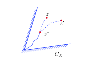
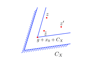
Figure 3.

Suppose the claim is proved. Take any $v^{\prime}=(v_{1}^{\prime},\dots,v_{m}^{\prime})\in A(z^{\prime}-z^{*})$ and set $v=u^{*}+v^{\prime}$. Then $v\in A(z^{\prime})$ and

$$\|u-v\|_{\infty} \leq \|u-u^{*}\|_{\infty}+\|v-u^{*}\|_{\infty}$$

$$\leq (\|z-z^{*}\|+\|z^{\prime}-z^{*}\|)/\delta\quad(\text{By Lemma \ref{lem-3.1}})$$

$$\leq (2M^{\prime}+C_{0})/\delta.$$

We have thus proved the theorem by choosing $M=\sqrt{m}(2M^{\prime}+C_{0})/\delta$.

Now it suffices to prove the claim. Take $x_{0}\in\mathcal{J}$ such that $B(x_{0},C_{0})\subset{\mathbf{C}}_{X},$ where $B(x,r)$ denotes the ball with center $x$ and radius $r$. Take $g\in\mathcal{J}$ such that $g+{\mathbf{C}}_{X}$ is a saturated cone. We will prove the claim by distinguishing two cases according to whether $z\in g+x_{0}+{\mathbf{C}}_{X}$.

Case 1: $z\in g+x_{0}+{\mathbf{C}}_{X}.$

A point $\tilde{z}=\sum_{j=1}^{m}\tilde{u}_{j}X_{j}$ is called a first entering position if $\tilde{u}=(\tilde{u}_{1},\dots,\tilde{u}_{m})$ is a minimal vector (w.r.t. the order $\preceq$) such that $\tilde{z}\in g+x_{0}+{\mathbf{C}}_{X}$ and $\tilde{u}\preceq u$. Such $\tilde{z}$ do exist, but may not be unique (See Figure 3 right). We fix such a point $\tilde{z}$ and set $z^{*}=z-\tilde{z}$. Since $\tilde{u}\preceq u$, we have $z^{*}\in\mathcal{J}$. We are going to check that (i)-(iii) hold for this $z^{*}$.

(i) holds since $\tilde{u}\preceq u$.

From $z-z^{*}=\tilde{z}\in g+x_{0}+{\mathbf{C}}_{X}$ we deduce that $z-z^{*}-x_{0}\in g+{\mathbf{C}}_{X}$. This, together with $\|z-z^{\prime}\|\leq C_{0}$, implies

$$z^{\prime}-z^{*}\in B(z,C_{0})-z^{*}=z-z^{*}-x_{0}+B(x_{0},C_{0})\subset(z-z^{*}-x_{0})+{\mathbf{C}}_{X}\subset g+{\mathbf{C}}_{X}.$$

Hence $z^{\prime}-z^{*}\in(g+{\mathbf{C}}_{X})\cap\mathcal{L}$, and so that $z^{\prime}-z^{*}\in{\mathcal{J}}$ by the saturation property of $g+C_{X}$. This proves the property (ii).

Recall that $\tilde{z}\in g+x_{0}+{\mathbf{C}}_{X}$. The minimality of $\tilde{z}$ implies

$$\tilde{z}\in(g+x_{0})+\left\{\sum_{j=1}^{m}c_{j}X_{j};0\leq c_{j}<1\right\}.$$

It follows that

$$\|z-z^{*}\|=\|\tilde{z}\|\leq\|g+x_{0}\|+\sum_{j=1}^{m}\|X_{j}\|:=M^{\prime},$$

and hence (iii) holds.

Case 2. $z\not\in g+x_{0}+{\mathbf{C}}_{X}.$

In this case, we could say that $z$ is close to a face of the cone ${\mathbf{C}}_{X}$. Indeed, the boundary of ${\mathbf{C}}_{X}$ can be written as

$$\partial{\mathbf{C}}_{X}=\bigcup_{j=1}^{N}{\mathcal{D}}_{j},$$

where ${\mathcal{D}}_{j}$ are faces of ${\mathbf{C}}_{X}$, which are cones of dimension $s-1$. Let $\vec{n}_{j}$ be the unit vector perpendicular to ${\mathcal{D}}_{j}$ and pointing to the half-space containing ${\mathbf{C}}_{X}$, that is to say, $\langle\vec{n}_{j},x\rangle\geq 0$ for all $x\in{\mathbf{C}}_{X}.$ We note that $x\in{\mathbf{C}}_{X}$ if and only if $\langle\vec{n}_{j},x\rangle\geq 0$ for all $j\in\{1,\dots,N\}.$

Since $z\not\in g+x_{0}+{\mathbf{C}}_{X},$ there exists an integer $j_{0}\in\{1,\dots,N\}$ such that $\langle\vec{n}_{j_{0}},z-(g+x_{0})\rangle<0$, namely,

(3.4) $$\langle z,\vec{n}_{j_{0}}\rangle<\langle g+x_{0},\vec{n}_{j_{0}}\rangle,$$

which means that $z$ is closer to the face ${\mathcal{D}}_{j_{0}}$ than $g+x_{0}$. Let $\Omega_{j_{0}}=\{i;~{}\langle X_{i},\vec{n}_{j_{0}}\rangle=0\}$. Take any $u=(u_{1},\dots,u_{m})\in A(z)$ and set

$$z_{1}=\underset{i\in\Omega_{j_{0}}}{\sum}u_{i}X_{i}.$$

Clearly, $z_{1}\in{\mathcal{D}_{j_{0}}}$. Denote $\delta^{\prime}=\min\{\langle X_{i},\vec{n}_{j_{0}}\rangle;i\in\{1,\dots,m\}\setminus\Omega_{j_{0}}\}.$ Since $\langle X_{j},\vec{n}_{j_{0}}\rangle\geq 0$ for all $j\in\{1,2,\cdots,m\}$, we deduce that for all $i\in\{1,\dots,m\}\setminus\Omega_{j_{0}}$ we have

$$u_{i}\leq\frac{\langle z,\vec{n}_{j_{0}}\rangle}{\delta^{\prime}}\leq\frac{\langle g+x_{0},\vec{n}_{j_{0}}\rangle}{\delta^{\prime}}:=M_{1}.$$

It follows that

(3.5) $$\|z-z_{1}\|\leq mM_{1}\underset{1\leq j\leq m}{\max}\|X_{j}\|.$$

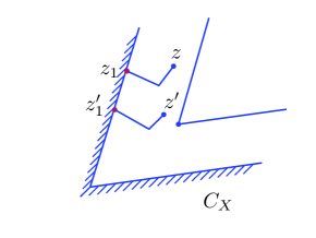
Figure 4.

Take any $v=(v_{1},\dots,v_{m})\in A(z^{\prime})$ and set $z^{\prime}_{1}=\underset{i\in\Omega_{j_{0}}}{\sum}v_{i}X_{i}.$ Then $z^{\prime}_{1}\in{\mathcal{D}_{j_{0}}}$. A similar argument as above shows that $v_{i}\leq M_{1}+C_{0}/\delta^{\prime}:=M_{2},\ \text{for all }\ i\in\{1,\dots,m\}\setminus\Omega_{j_{0}},$ and

(3.6) $$\|z^{\prime}-z^{\prime}_{1}\|\leq mM_{2}\underset{1\leq j\leq m}{\max}\|X_{j}\|.$$

According to (3.5) and (3.6), to prove the claim holds for $z$ and $z^{\prime}$, we only need prove that the claim hold for $z_{1}$ and $z_{1}^{\prime}$. That is say, suppose we can walk from the origin to a suitable point $z_{1}^{*}$ and then walk from $z_{1}^{*}$ to $z_{1}$ as well as to $z_{1}^{\prime}$. These walks remains in the lower dimensional cone ${\mathcal{D}}_{j_{0}}$. Of cause, we can finally walk to $z$ and to $z^{\prime}$. Observe that

$$\|z_{1}-z^{\prime}_{1}\|<m(M_{1}+M_{2})\underset{1\leq j\leq m}{\max}\|X_{j}\|+C_{0}.$$

The claim can thus be proved by induction on the dimension of the cone. ∎

The following theorem asserts that $\mathbf{m}(z)$ varies not so rapidly. Theorem 3.2 will be useful for its proof.

Theorem 3.3.

Let $C_{0}\geq 1$ be an integer. There exists a polynomial $Q(x)$ with positive coefficients such that

$$\frac{1}{Q(\|z\|)}\leq\frac{{\mathbf{m}}(z)}{{\mathbf{m}}({z^{{}^{\prime}}})}\leq Q(\|z\||)$$

provided that $z,z^{\prime}\in{\mathcal{J}}$ and $\|z-z^{\prime}\|\leq C_{0}.$

Proof.

Let $M$ be the constant in Theorem 3.2, which depends on $C_{0}$. There exists a polynomial $G(x)$ (depending on $m$ and $M$) with positive coefficients such that

$$\frac{|v|!}{|u|!}\cdot\frac{u!}{v!}\leq G(\|u\|)$$

holds for all $u,v\in\mathbb{N}^{m}$ such that $\|u-v\|\leq M$. In other word,

$$\frac{|u|!}{u!}\geq\frac{1}{G(\|u\|)}\frac{|v|!}{v!}.$$

We can take $G(x)=x^{2mM}$. Denoting by $N_{0}$ the number of integer points in the ball $B(0,M)$, we have

(3.7) $$N_{0}\frac{|u|!}{u!}\geq\frac{1}{G(\|u\|)}\underset{v:\|u-v\|\leq M}{\sum}\frac{|v|!}{v!}.$$

Summing up both sides of (3.7) over $u\in A(z)$, we obtain

(3.8) $$N_{0}\underset{u\in A(z)}{\sum}{\frac{|u|!}{u!}}\geq\frac{1}{G(\|u^{*}\|)}\underset{u\in A(z)}{\sum}\left(\underset{v:\|u-v\|\leq M}{\sum}\frac{|v|!}{v!}\right)\geq\frac{1}{G(\|u^{*}\|)}\underset{v\in A(z^{\prime})}{\sum}\frac{|v|!}{v!},$$

where $u^{*}$ is a point in $A(z)$ such that $\|u^{*}\|$ attains the maximum. The last inequality holds because

$$A(z^{\prime})\subset\underset{u\in A(z)}{\bigcup}\{v\in{\mathbb{N}}^{s};~{}\|u-v\|\leq M\}$$

by Theorem 3.2. By recalling the expression (3.2) for $\mathbf{m}(z)$, we see that (3.8) is nothing but

$$\frac{\mathbf{m}(z)}{\mathbf{m}(z^{\prime})}\geq\frac{1}{N_{0}G(\|u^{*}\|)}.$$

Since $\|u^{*}\|\leq m\|u^{*}\|_{\infty}\leq m\|z\|/\delta$ (by Lemma 3.1), where $\delta$ is defined by (3.3), we have

$$\frac{1}{N_{0}G(m\|z\|/\delta)}\leq\frac{\mathbf{m}(z)}{\mathbf{m}(z^{\prime})}\leq N_{0}G(m\|z^{\prime}\|/\delta)$$

where the second inequality is obtained from the first one by symmetry. Notice that $\|z^{\prime}\|\leq\|z\|+C_{0}$. We have thus proved the theorem with $Q(x)=N_{0}G\left(\delta^{-1}{m(x+C_{0})}\right)$. ∎

4. Existence of directional growth

In this section we prove the existence of the limit defining the directional growth $\gamma(\theta)$. Recall that the multiplicity of a point in ${\mathbf{C}}_{X}$ is defined as

$${\mathbf{m}}(x)=\min\{{\mathbf{m}}(z):\ z\in{\mathcal{J}}\text{ and }\|x-z\|=d(x,{\mathcal{J}})\}.$$

Proof of Theorem 1.2. Fix a unit vector $\theta$ in ${\mathbf{C}}_{X}$. Let us denote $z_{k}$ to be the point in $\mathcal{J}$ such that

$$\mathbf{m}(k\theta)=\mathbf{m}(z_{k}),\quad d(k\theta,z_{k})=d(k\theta,\mathcal{J}).$$

By the relative density of ${\mathcal{J}}$ (Lemma 2.2), there exists a constant $R_{0}>0$ such that

(4.1) $$\|z_{k}-k\theta\|<R_{0}$$

for all $k$ and all $\theta$. By the definition of multiplicity, it is obvious that $\mathbf{m}(z+z^{\prime})\geq\mathbf{m}(z)\mathbf{m}(z^{\prime})$ for any $z,z^{\prime}\in{\mathcal{J}}$. In particular, for any $n,p\geq 1$,

(4.2) $$\mathbf{m}(z_{n}+z_{p})\geq\mathbf{m}(z_{n})\mathbf{m}(z_{p}).$$

As consequence of (4.1), we have $\|z_{n+p}-(z_{n}+z_{p})\|\leq 3R_{0}.$ Hence, by Theorem 3.3, there exists a polynomials $Q(x)$ with positive coefficients such that

$$\mathbf{m}(z_{n+p})\geq\frac{1}{Q(\|z_{n+p}\|)}\mathbf{m}(z_{n}+z_{p})\geq\frac{1}{Q(\|z_{n+p}\|)}\mathbf{m}(z_{n})\mathbf{m}(z_{p}).$$

Using the fact $\mathbf{m}(k\theta)=\mathbf{m}(z_{k})$ for all $k$, we get then

$$\mathbf{m}((n+p)\theta)\geq\frac{1}{\widetilde{Q}(n+p)}\mathbf{m}(n\theta)\mathbf{m}(p\theta),$$

where $\widetilde{Q}(x)=Q(x+R_{0})$. Here we used the observation that $\|z_{n+p}\|\leq(n+p)+R_{0}$ and the fact that $Q(x)$ has positive coefficients to get $Q(\|z_{n+p}\|)\leq\widetilde{Q}(n+p)$. Observe that $\log\widetilde{Q}(n+p)\leq c\log(n+p)$ for some constant $c>0$. We can finish the proof by using the next lemma to $b_{n}=\log\mathbf{m}(n\theta)$.  $\Box$

It is well known that if a sequence $b_{n}$ is sub-additive, i.e., $b_{n}+b_{m}\leq b_{n+m}$, then the limit $\lim b_{n}/n$ exists. The following lemma strengthen this result.

Lemma 4.1.

Let $c>0$ be a constant. If $\{b_{n}\}$ be a sequence in $\mathbb{R}^{+}$ such that

(4.3) $$b_{n}+b_{m}\leq b_{n+m}+c\log(m+n),\quad\text{ for all }m,n\geq 1,$$

then the limit $\underset{n\rightarrow\infty}{\lim}b_{n}/n$ exists.

Proof.

Without loss of generality, we can assume $c=1$, otherwise we consider $c^{-1}b_{n}$ instead of $b_{n}$. Fix a positive integer $m$. By (4.3) we have

(4.4) $$\forall s\geq 1,\qquad b_{2^{s}m}\geq 2b_{2^{s-1}m}-\log(2^{s}m).$$

Fix a positive integer $l\geq 1$. For $1\leq s\leq l$, as consequence of (4.4) we get

(4.5) $$b_{2^{l}m}\geq 2^{l}b_{m}-[2^{l-1}\log(2m)+2^{l-2}\log(4m)+\cdots+\log(2^{l}m)]=2^{l}b_{m}-g(m,l)$$

where

$$g(m,l)=(2^{l+1}-2-l)\log 2+(2^{l}-1)\log m.$$

For any $n\in\mathbb{N},$ we write $n=Lm+r$ with $0\leq r<m$. By (4.3), we have

$$b_{n}\geq b_{Lm}+b_{r}-\log n.$$

In order to estimate $b_{Lm}$, we use $L$’s dyadic expansion $L=2^{l_{1}}+2^{l_{2}}+\dots+2^{l_{k}}$ where $l_{1}>l_{2}>\dots>l_{k}\geq 0$. Obviously $\log_{2}L-1\leq l_{1}\leq\log_{2}L$. Using (4.3) then (4.5), we obtain

$$b_{Lm} \geq b_{2^{l_{1}}m}+b_{(2^{l_{2}}+\dots+2^{l_{k}})m}-\log((2^{l_{1}}+2^{l_{2}}+\dots+2^{l_{k}})m)$$

$$\geq 2^{l_{1}}b_{m}-g(m,l_{1})-\log((2^{l_{1}}+2^{l_{2}}+\dots+2^{l_{k}})m)+b_{(2^{l_{2}}+\dots+2^{l_{k}})m}.$$

Hence, by induction, we have

$$b_{Lm}\geq\sum_{j=1}^{k-1}\left(2^{l_{j}}b_{m}-g(m,l_{j})-\log((2^{l_{j}}+\cdots+2^{l_{k}})m)\right)+2^{l_{k}}b_{m}-g(m,l_{k}).$$

Note that $\sum_{j=1}^{k}2^{l_{j}}=L$ and

$$\sum_{j=1}^{k}g(m,l_{j})\leq\sum_{j=1}^{k}2^{l_{j}}\log 4m\leq L\log(4m),$$

$$\sum_{j=1}^{k-1}\log((2^{l_{j}}+\cdots+2^{l_{k}})m)\leq l_{1}\log(Lm)\leq\log_{2}n\log n.$$

Hence we have

$$b_{Lm}\geq Lb_{m}-L\log 4m-\log_{2}n\log n.$$

Dividing both sides by $n$, taking the liminf and using the fact $L/n\to m$, we have

(4.6) $$\underset{n\rightarrow\infty}{\liminf}\ \frac{b_{n}}{n}\geq\frac{b_{m}-\log 4m}{m}.$$

Then taking the limsup as $m\to\infty$ finishes the proof. ∎

5. Principle of Maximal entropy under linear constraints

Let $\Delta_{m}$ be the simplex of all probability measures $p=(p_{1},\dots,p_{m})$. The entropy function $h(p)$ is defined on $\Delta_{m}$ as follows

$$h(p)=-\sum_{j=1}^{m}p_{j}\log p_{j}.$$

Let $X_{1},\cdots,X_{m}$ be $m$ given vectors in a Euclidean space $\mathbb{R}^{d}$. We will consider the maximum of $h(p)$ under the constraints

(5.1) $$\sum_{j=1}^{m}p_{j}=1,\qquad\sum_{j=1}^{m}p_{j}X_{j}=\beta$$

for any $\beta$ in the convex hull generated by $X=\{X_{1},\cdots,X_{m}\}$ which is defined by

$$\Delta_{X}=\left\{\sum_{j=1}^{m}p_{j}X_{j}:(p_{1},\cdots,p_{m})\in\Delta_{m}\right\}.$$

When $d=1$, the solution is given by the principle of maximum entropy due to Jaynes [9].

Let us define

$$Z(t)=\sum_{j=1}^{m}e^{\langle t,X_{j}\rangle},\qquad t\in\mathbb{R}^{d}.$$

We have

$$\nabla Z(t)=\sum_{j=1}^{m}X_{j}e^{\langle t,X_{j}\rangle}$$

Theorem 5.1.

Suppose that the vectors $X_{1},\cdots,X_{m}$ are not coplanar and $\beta$ is in the interior of $\Delta_{X}$. Then under the constraints $\sum_{j=1}^{m}p_{j}=1$ and $\sum_{j=1}^{m}p_{j}X_{j}=\beta$, the entropy function $h(p)$ attains its maximum at the maximal point $p^{*}$ defined by

(5.2) $$p_{j}^{*}=\frac{e^{\langle t_{\beta},X_{j}\rangle}}{Z(t_{\beta})}\qquad(j=1,2,\cdots,m)$$

where $t_{\beta}$ is the unique solution of the equation

(5.3) $$\frac{\nabla Z(t)}{Z(t)}=\beta.$$

Actually the maximal point is unique and the maximum entropy is equal to

$$h(p^{*})=\log Z(t_{\beta})-\langle t_{\beta},\beta\rangle.$$

The map $\beta\mapsto t_{\beta}$ is $C^{\infty}$-diffeomorphism from $\stackrel{{\scriptstyle\circ}}{{\Delta}}_{X}$ onto $\mathbb{R}^{d}$.

The proof of the theorem will be decomposed into several lemmas.

We will denote by $\stackrel{{\scriptstyle\circ}}{{A}}$ the interior of a set $A$. Let $M:\mathbb{R}^{m}\to\mathbb{R}^{d}$ the linear map defined by the $d\times m$ matrix

$$M=\left(X_{1},\dots,X_{m}\right).$$

Lemma 5.2.

$\stackrel{{\scriptstyle\circ}}{{\Delta}}_{X}=M(\stackrel{{\scriptstyle\circ}}{{\Delta}}_{m}).$

Proof.

Notice that $Mp=\sum_{j=1}^{m}p_{j}X_{j}$. Let $\pi:\mathbb{R}^{m}\to\mathbb{R}^{m}/_{\mbox{\rm ker}(M)}$ be the canonical map from $\mathbb{R}^{m}$ to the quotient space $\mathbb{R}^{m}/_{\mbox{\rm ker}(M)}$ and let $\widetilde{M}$ be the compatible map such that $M=\widetilde{M}\circ\pi$. Since the map $\pi$ is open and the map $\widetilde{M}$ is a homeomorphism, the subset $M(\stackrel{{\scriptstyle\circ}}{{\Delta}}_{m})$ of $\Delta_{X}$ is open, so that $M(\stackrel{{\scriptstyle\circ}}{{\Delta}}_{m})\subset\stackrel{{\scriptstyle\circ}}{{\Delta}}_{X}$.

On the other hand, the compact convex set $\Delta_{X}$ admits its extremal points among $\{X_{1},\cdots,X_{m}\}$. We first claim that any extremal point, say $X_{1}$, is a limit point of $M(\stackrel{{\scriptstyle\circ}}{{\Delta}}_{m})$. In fact, since $X_{1}-X_{j}$ ($j=2,\cdots,m$) are in a half-space, there is a vector $h\in\mathbb{R}^{d}$ such that $\langle h,X_{1}-X_{j}\rangle>0$ for all $j=2,\cdots,m$. Then the points

$$Y_{n}=\frac{\nabla Z(nh)}{Z(nh)}\in M(\stackrel{{\scriptstyle\circ}}{{\Delta}}_{m})$$

tend to $X_{1}$ (the argument holds even if some of $X_{j}$ ($j\geq 2$) are equal to $X_{j}$, such a case was not excluded). To finish the proof, it suffices to observe that any $\beta\in\stackrel{{\scriptstyle\circ}}{{\Delta}}_{X}$ is a convex combination with strict positive coefficients of a set of points in $\stackrel{{\scriptstyle\circ}}{{\Delta}}_{X}$, each of which is sufficiently close to an extremal point of ${\Delta}_{X}$. It follows that $\beta\in M(\stackrel{{\scriptstyle\circ}}{{\Delta}}_{m})$. ∎

The constraints (5.1) define a compact set on which the entropy function which is continuous attains its maximum. We will show that the entropy function attains its maximum at an interior point and the maximal point is unique if $\beta\in\stackrel{{\scriptstyle\circ}}{{\Delta}}_{X}$.

Lemma 5.3.

Assume $\beta\in\stackrel{{\scriptstyle\circ}}{{\Delta}}_{X}$. Under the constraints (5.1), the entropy attains its maximum at a point $p^{*}\in\stackrel{{\scriptstyle\circ}}{{\Delta}}_{m}$. Such maximal points are unique.

Proof.

The uniqueness of maximal points is just because of the strict concavity of the entropy function.

Let $p^{*}$ be the maximal point. Suppose that $p^{*}$ is not strictly positive. Without loss of generality, we assume that $p_{j}^{*}>0$ for $j=1,\dots,k$, but $p_{j}^{*}=0$ for $j=k+1,\dots,m$. Since $\beta\in\stackrel{{\scriptstyle\circ}}{{\Delta}}_{X}$, by Lemma 5.2, there exists a probability vector $q\in\stackrel{{\scriptstyle\circ}}{{\Delta}}_{m}$ such that $\beta=Mq$. Denote $r=q-p^{*}$. Then we have $Mr=0$. Notice that $\sum_{i=1}^{m}r_{i}=0$ and $r_{j}>0$ for $j=k+1,\dots,m$. Consider the perturbation of $p^{*}$ defined by

$$p_{t}={p^{*}+tr}.$$

For small $t>0$, $p_{t}$ is a probability satisfying the constraint $Mp_{t}=\beta$. Then consider of function $f(t)=h(p_{t})$, that is

$$f(t)=-\sum_{j=1}^{m}(p^{*}_{j}+tr_{j})\log(p_{j}^{*}+tr_{j}).$$

Its derivative is equal to

$$f^{\prime}(t)=-\sum_{j=1}^{m}r_{j}\left(\log(p_{j}^{*}+tr_{j})+1\right).$$

Let $\epsilon=\min_{1\leq j\leq k}p_{j}^{*}$. Then for $t$ small enough, we have

$$-r_{j}(\log(p_{j}^{*}+tr_{j})+1)\geq|r_{j}|(\log\epsilon/2+1),\qquad\text{ for }j=1,\dots,k;$$

but as $t\to 0^{+}$,

$$-r_{j}(\log(p_{j}^{*}+tr_{j})+1)=-r_{j}\log(tr_{j})-r_{j}\to\infty,\qquad\text{ for }j=k+1,\dots,m.$$

So we have $f^{\prime}(t)>0$ for small $t>0$ and hence $f(t)$ is increasing near $0$. This contradicts the maximality of $h(p^{*})$. ∎

Lemma 5.4.

There exists a unique point $t_{\beta}\in\mathbb{R}^{d}$ such that

(5.4) $$p^{*}_{j}=\frac{e^{\langle t_{\beta},X_{j}\rangle}}{Z(t_{\beta})},\qquad 1\leq j\leq m.$$

This point $t_{\beta}$ is the unique solution of the equation $\nabla Z(t)/Z(t)=\beta$. The maximal entropy $h(p^{*})$ is equal to $\log Z(t_{\beta})-\langle t_{\beta},\beta\rangle$.

Proof.

Consider the function

$$F(p,\lambda,t)=h(p)+\lambda\left(\sum_{j=1}^{m}p_{j}-1\right)+\left\langle t,\sum_{j=1}^{m}p_{j}X_{j}-\beta\right\rangle$$

where $p\in{(\mathbb{R}^{+})}^{m}$, $\lambda\in\mathbb{R}$ and $t\in\mathbb{R}^{d}$. Both $\lambda$ and $t$ are Lagrange multipliers. The maximal point $p^{*}$ whose existence is proved above must be the critical point of $F$. But

$$\frac{\partial F}{\partial p_{j}}=-\log p_{j}-1+\lambda+\langle t,X_{j}\rangle.$$

We deduce that the maximal point $p^{*}$ is of the form

(5.5) $$p_{j}^{*}=\frac{e^{\langle t,X_{j}\rangle}}{Z(t)}$$

for some $t$ verifying $\nabla Z(t)/Z(t)=\beta$. By the way, we have proved that the equation $\nabla Z(t)/Z(t)=\beta$ admits a solution. We claim that there is a unique $t$ verifying (5.5). Suppose $t^{\prime}\not=t$ is another suitable point. Then

$$\frac{e^{\langle t,X_{j}\rangle}}{Z(t)}=\frac{e^{\langle t^{\prime},X_{j}\rangle}}{Z(t^{\prime})},\qquad i.e.\ \ \ e^{\langle t-t^{\prime},X_{j}\rangle}=\frac{Z(t)}{Z(t^{\prime})}.$$

Then $e^{\langle t-t^{\prime},X_{i}-X_{j}\rangle}=1$, i.e. $\langle t-t^{\prime},X_{i}-X_{j}\rangle=0$ for all $i,j$. This contradicts that $X_{j}$’s are not coplanar. Clear $h(p^{*})=\log Z(t_{\beta})-\langle t_{\beta},\beta\rangle$ where $t_{\beta}$ is the unique point satisfying (5.5).

Now we prove that the equation $\nabla Z(t)/Z(t)=\beta$ admits a unique solution. Suppose that $t^{\prime}$ is another solution. We can check that the probability $p^{\prime}$ defined by $p^{\prime}_{j}=e^{\langle t^{\prime},X_{j}\rangle}/Z(t^{\prime})$ is a maximal point. So, $p^{\prime}=p^{*}$ and then $t^{\prime}=t$. ∎

Consider $t_{\beta}$ as a function of $\beta\in\stackrel{{\scriptstyle\circ}}{{C}}_{X}$. It is the inverse function of $t\mapsto A(t)$ where

$$A(t)=\frac{\nabla Z(t)}{Z(t)}.$$

Lemma 5.5.

The differential $dA(t)$ is non-singular at any point $t\in\mathbb{R}^{d}$. Hence $\beta\mapsto t_{\beta}$ is infinitely differentiable.

Proof.

Let $p(t)$ be the probability vector defined by $\nabla Z(t)/Z(t)$. Define the $m\times m$ matrix

$$G(t)=\text{diag~{}}(p(t))-p(t)\cdot p(t)^{T},$$

where $\text{diag~{}}(p(t))$ denotes the diagonal matrix with the elements of $p(t)$ as diagonal elements and $p(t)^{T}$ denotes the transpose of the column vector $p(t)$. A direct calculation shows that

$$dA(t)=MG(t)M^{T}.$$

Observe that $G(t)$ is symmetric and it defines the quadratic form

$$yG(t)y^{T}=\sum_{j=1}^{m}p_{j}y_{j}^{2}-\left(\sum_{j=1}^{m}p_{j}y_{j}\right)^{2}.$$

If we introduce the inner product $(x,y)=\sum_{j=1}^{m}p_{j}x_{j}y_{j}$, by the Cauchy inequality we see that $G(t)$ is positive and $yG(t)y^{T}=0$ iff $y$ is parallel to $(1,1,\cdots,1)$.

Suppose that $dA(t)$ is singular. Then $xMG(t)M^{T}x^{T}=0$ for some $x\in\mathbb{R}^{d}$ with $x\neq 0$, i.e. $yG(t)y^{T}=0$ for $y=xM$. By the properties of $G(t)$ proved above, $xM=c(1,1,\dots,1)$ for some $c\not=0$, which means $\langle x,X_{j}\rangle=c$ for all $j$, i.e. $X_{1},\dots,X_{m}$ are coplanar. This is a contradiction. The infinite differentiability is a consequence of the implicit function theorem. ∎

Finally, we consider the case that $X_{1},\dots,X_{m}$ are coplanar. Let $H_{0}$ be the subspace spanned by $X_{i}-X_{j}$ ($i,j=1,2,\cdots,m$). Then $s:=\dim H_{0}<d$. We can apply the theorem if we replace $\mathbb{R}^{d}$ by $H_{0}$ and $t$ by vectors in $H_{0}$. Then there is a unique $t_{\beta}$ in $H_{0}$ associated to $\beta\in\stackrel{{\scriptstyle\circ}}{{C}}_{X}$. We can also consider $t\in\mathbb{R}^{d}$. Then consider the orthogonal decomposition $\mathbb{R}^{d}=H_{0}\oplus H_{0}^{\bot}$. For each $\beta\in\stackrel{{\scriptstyle\circ}}{{C}}_{X}$, the solution of the equation $\nabla Z(t)/Z(t)=\beta$ is the set $t_{\beta}+H_{0}^{\bot}$ where $t_{\beta}\in H_{0}$.

6. Formula of $\gamma(\theta)$ in the coplanar case

In this section, we prove an formula for the growth function $\gamma$ when $X_{1},\cdots,X_{m}$ are coplanar. Let $\eta$ be a non zero vector in $\mathbb{R}^{s}$, considered as the normal direction of a hyperplane. Recall that $X_{1},\dots,X_{m}$ are $\eta$-coplanar if

(6.1) $$\forall j\in\{1,\dots,m\},\quad\langle X_{j},\eta\rangle=1.$$

Denote by $H_{\eta}=\{X\in\mathbb{R}^{s}:\langle X,\eta\rangle=1\}$ the hyperplane containing $X_{1},\cdots,X_{m}$. By the discussion of the previous section, we have

Lemma 6.1.

If $\beta$ is an interior point in $H_{\eta}\cap{\mathbf{C}}_{X}$, then the solution $t$ of the equation (5.3) exists and is unique up to a difference of $c\eta$ with $c\in\mathbb{R}$. Moreover, the entropy function $h(p)=-\sum_{j=1}^{m}p_{j}\log p_{j}$ with the constraint

(6.2) $$p_{1}X_{1}+\cdots+p_{m}X_{m}=\beta.$$

attains it maximum at

(6.3) $$p_{j}=\frac{e^{\langle t,X_{j}\rangle}}{Z(t)},\qquad 1\leq j\leq m.$$

The function $Z(t)$ is conventionally called partition function and the probability given by (6.3) is called Gibbs distribution.

The vector $t$ depends on $\beta$. In the following, we will consider $\beta=\frac{\theta}{\langle\theta,\eta\rangle}$, so $t$ will depends on $\theta$.

Proof of Theorem 1.3. For a fixed unit vector $\theta$ in the cone ${\bf C}_{X}$, put $\displaystyle\beta=\frac{\theta}{\langle\theta,\eta\rangle}$, which is the point on the hyperplane $H_{\eta}$ of the direction $\theta$.

Lower bound of $\gamma(\theta)$. Take any probability vector $p$ satisfying the constraint (6.2). Let

(6.4) $$n_{j}=\lfloor np_{j}\rfloor,\text{ for }j=1,\dots,m-1\text{ and }n_{m}=n-(n_{1}+\cdots+n_{m-1}).$$

It is clear that there exists a constant $c$ independent of $n$ (for example, $c=3m\sum_{j=1}^{m}\|X_{j}\|$) such that

(6.5) $$\left\|\sum_{j=1}^{m}n_{j}X_{j}-n\beta\right\|\leq c,\qquad\sum_{j=1}^{m}|n_{j}-np_{j}|\leq c.$$

So, applying Theorem 3.3 with $C_{0}=2c$, we have

$$Q(n\|\beta\|)\mathbf{m}(n\beta)\geq\mathbf{m}\left(\sum_{j=1}^{m}n_{j}X_{j}\right)\geq\frac{n!}{n_{1}!\dots n_{m}!}\sim\frac{n!}{(np_{1})!\dots(np_{m})!},$$

where $Q(x)$ is the polynomial in Theorem 3.3, and $A\sim B$ means that $A/B$ and $B/A$ are bounded by a polynomial of $n$. Using Stirling’s formula, we obtain that

$$\lim_{n\to\infty}\frac{\log\mathbf{m}(n\beta)}{n}\geq\log\frac{1}{p_{1}^{p_{1}}\cdots{p_{m}}^{p_{m}}}=h(p).$$

Therefore

$$\gamma(\theta) = \lim_{k\to\infty}\frac{\log\mathbf{m}(k\theta)}{k}=\langle\theta,\eta\rangle\lim_{n\to\infty}\frac{\log\mathbf{m}(n\beta)}{n}\geq\langle\theta,\eta\rangle h(p).$$

Taking the supremum we get the following lower bound for $\gamma(\theta)$

$$\gamma(\theta)\geq\langle\theta,\eta\rangle\sup\left\{h(p):~{}p_{1}X_{1}+\cdots+p_{m}X_{m}=\beta\right\}.$$

Upper bound of $\gamma(\theta)$. Let $p$ be a probability vector such that $h(p)$ attains maximum under the restriction (6.2). Let $(n_{1},\dots,n_{m})$ be the vector defined by (6.4). Let $x_{n}=n_{1}X_{1}+\cdots+n_{m}X_{m}$. Then $|x_{n}-n\beta|\leq c$. Since $p$ is the Gibbs distribution which is of exponential form (see (6.3)), for any $(n_{1}^{\prime},\dots,n_{m}^{\prime})$ satisfying $n_{1}^{\prime}X_{1}+\cdots+n_{m}^{\prime}X_{m}=x_{n}$, we have

$$p_{1}^{n_{1}^{\prime}}\cdots p_{m}^{n_{m}^{\prime}}=\frac{\exp\langle t,n_{1}^{\prime}X_{1}+\cdots+n_{m}^{\prime}X_{m}\rangle}{Z(t)^{n}}=\frac{\exp\langle t,x_{n}\rangle}{Z(t)^{n}}.$$

Now we consider a random walk: at any time, we forward the step $X_{j}$ with the probability $p_{j}$. Then the above formula says that for any $\omega,\omega^{\prime}\in\{1,2,\cdots,m\}^{n}$, as soon as $\kappa(\omega)=\kappa(\omega^{\prime})$, both $\omega$ and $\omega^{\prime}$ have the same probability. It follows that $Z(t)^{-n}\exp\langle t,x_{n}\rangle\mathbf{m}(x_{n})$ is bounded by the probability that we arrive at $x_{n}$ at time $n$, which is bounded by $1$. Hence,

$$\mathbf{m}(x_{n})\leq\frac{Z(t)^{n}}{\exp\langle t,x_{n}\rangle}=\frac{1}{p_{1}^{n_{1}}\cdots p_{m}^{n_{m}}}.$$

As $n_{j}/n\to p_{j}$, we have

$$\lim_{n\to\infty}\frac{\log\mathbf{m}(x_{n})}{n}\leq h(p).$$

Finally, since $\mathbf{m}(n\beta)/\mathbf{m}(x_{n})$ is controlled by a polynomial of $n$, we obtain

$$\gamma(\theta)=\langle\theta,\eta\rangle\lim_{n\to\infty}\frac{\log\mathbf{m}(n\beta)}{n}\leq\langle\theta,\eta\rangle h(p).$$

This ends the proof of the theorem. $\Box$

Theorem 6.2.

If $X_{1},\dots,X_{m}$ are $\eta$-coplanar, then for any unit vector $\theta$ in the interior of ${\bf C}_{X}$ we have

$$\gamma(\theta)=\langle\theta,\eta\rangle\log Z(t)-\langle t,\theta\rangle$$

where $t$ is any solution stated in Lemma 6.1.

Proof.

As we have seen in the above proof of Theorem 1.3, the supremum is attained at the Gibbs distribution $p_{j}=e^{\langle t,X_{j}\rangle}Z(t)^{-1}$. Taking the logarithm, we get

$$-\log p_{j}=\log Z(t)-\langle t,X_{j}\rangle.$$

Multiplying both sides by $p_{j}$ and summing over $j$ allow us to get

$$h(p)=\log Z(t)-\sum_{j=1}^{m}p_{j}\langle t,X_{j}\rangle=\log Z(t)-\langle t,\beta\rangle$$

where $\beta=\theta/\langle\theta,\eta\rangle$. Finally, we obtain the formula by multiplying $\langle\theta,\eta\rangle$. ∎

The following proposition is an easy consequence of Theorem 1.3.

Proposition 6.3.

Assume that $X_{1},\dots,X_{m}$ are $\eta$-coplanar. Then

$$\max\frac{\gamma(\theta)}{\langle\eta,\theta\rangle}=\log m\text{ at }\theta_{0}=\frac{\sum_{j=1}^{m}X_{j}}{|\sum_{j=1}^{m}X_{j}|}.$$

The reason is that the entropy $h(p)$ attains its maximum $\log m$ at $p_{1}=\cdots=p_{m}=1/m$. The corresponding direction on the hyperplane $H_{\eta}$ is $\beta_{0}=\frac{1}{m}\sum_{j=1}^{m}X_{j}$, the arithmetic average of $X_{1},X_{2},\cdots,X_{m}$. The corresponding unit vector is $\theta_{0}$.

The growth of the semi-group has been defined as function of the unit vector $\theta$. If we define the growth $\tilde{\gamma}(\beta)$ as function of the vector $\beta$ located on the hyperplane $H_{\eta}$, we will get a simpler formula

$$\tilde{\gamma}(\beta)=\sup\{h(p):p_{1}X_{1}+\cdots+p_{m}X_{m}=\beta\}=\log Z(t)-\langle t,\beta\rangle.$$

This is the conditional variation principle for the multifractal analysis of the Birkhoff average

(6.6) $$\lim_{n\to\infty}\frac{X_{\omega_{1}}+X_{\omega_{2}}+\cdots+X_{\omega_{n}}}{n}.$$

See [6, 7, 8] for discussion in more general case. In general, it is difficult to determine exactly the possible limits of the Birkhoff average. Theorem 1.3 shows that for the special case of (6.6), the possible limit is the convex set $H_{\eta}\cap{\bf C}_{X}$.

7. Rigidity (I): Proof of Theorem 1.5

When the vectors $X_{1},\cdots,X_{m}$ are $\eta$-coplanar, we have proved that the growth function is equal to

$$\gamma(\theta)=\langle\theta,\eta\rangle\left(\log Z(t)-\langle\beta,t\rangle\right)$$

where $\beta=\frac{\theta}{\langle\theta,\eta\rangle}$ and $t$ is any solution of the equation $\nabla Z(t)/Z(t)=\beta$. The set of solutions of $t$ is a line consisting of the points $t_{\beta}+c\eta$ ($c\in\mathbb{R}$) and we will choose the one such that the last coordinate of $t_{\beta}+c\eta$ is zero. It is really possible that the last coordinate is zero if $\eta_{s}\neq 0$. In fact, we can choose

$$c=-\frac{\langle t_{\beta},e_{s}\rangle}{\langle\eta,{\mathbf{e}}_{s}\rangle}$$

where ${\mathbf{e}}_{s}=(0,...,0,1)\in\mathbb{R}^{s}$. The next lemma shows that it is possible to convert the general case to the case with $\eta_{s}=:\langle\eta,e_{s}\rangle\not=0$.

Lemma 7.1.

Let $X=\{X_{1},\dots,X_{m}\}$ be a set of integral vectors on $\mathbb{Z}^{s}$ and let $T$ be an invertible $s\times s$ matrix with integral entries.
(i) The function $\gamma_{{}_{TX}}$ is related to $\gamma_{{}_{X}}$ by the formula

$$\gamma_{{}_{TX}}(\theta)=\|T^{-1}\theta\|\gamma_{{}_{X}}\left(\frac{T^{-1}\theta}{\|T^{-1}\theta\|}\right).$$

(ii) If $X$ is $\eta$-coplanar, then $TX$ is $(T^{*})^{-1}\eta$-coplanar, where $T^{*}$ is the transpose of $T$.

Proof.

(ii) is obvious. (i) is proved by computation. The key point is the observation $\mathbf{m}_{TX}(z)=\mathbf{m}_{X}(T^{-1}z)$. Then we have

$$\gamma_{{}_{TX}}(\theta) = \lim_{k\to\infty}\frac{\mathbf{m}_{TX}(k\theta)}{k}=\lim_{k\to\infty}\frac{\mathbf{m}_{X}(kT^{-1}\theta)}{k}$$

$$= \lim_{k\to\infty}\frac{\mathbf{m}_{X}(kT^{-1}\theta)}{\|kT^{-1}\theta\|}\cdot\frac{\|kT^{-1}\theta\|}{k}=\|T^{-1}\theta\|\gamma_{{}_{X}}\left(\frac{T^{-1}\theta}{\|T^{-1}\theta\|}\right).$$

∎

Theorem 1.5 and Theorem 1.6 compare two sets of vectors $X=\{X_{1},\cdots,X_{m}\}$ and $Y=\{Y_{1},\cdots,Y_{m^{\prime}}\}$, which are respectively $\eta$-coplanar and $\eta^{\prime}$-coplanar. Without loss of generality, we may assume that $\eta_{s}\neq 0$ and $\eta^{\prime}_{s}\neq 0$. Otherwise we can consider the images of $X$ and $Y$ under a linear transformation $T$ as stated in the last lemma. Actually, we may choose $a=(a_{1},\cdots,a_{s-1},1)\in\mathbb{Z}^{s}$ such that

$$\langle a,\eta\rangle\not=0,\quad\langle a,\eta^{\prime}\rangle\not=0.$$

Such $a$’s do exist, because the condition $\langle z,\eta\rangle=0$ or $\langle z,\eta^{\prime}\rangle=0$ defines a union of two hyperplanes and we can find points $a$ outside these two hyperplanes. Define

$$T=\left(\begin{array}[]{ccccc}1&&&&\ -a_{1}\\ &\ 1&&&-a_{2}\\ &&\ \ddots&&\vdots\\ &&&\ 1&-a_{s-1}\\ &&&&1\\ \end{array}\right).$$

Then we have the last coordinate of $T^{*-1}\eta$ is equal to $\langle a,\eta\rangle\not=0$ and the last coordinate of $T^{*-1}\eta^{\prime}$ is equal to $\langle a,\eta^{\prime}\rangle\not=0$.

From now on, we assume that $X_{1},\dots,X_{m}$ are $\eta$-coplanar vectors in $\mathbb{Z}^{s}$ such that $\eta_{s}\neq 0$ and that there is a (unique) solution $t$ of (5.3), i.e.

(7.1) $$\sum_{j=1}^{m}(X_{j}-\beta)e^{\langle t,X_{j}\rangle}=0$$

such that $t_{s}=0$. We define

$$F(\beta)=\log Z(t)-\langle\beta,t\rangle,$$

which is a function on $\beta_{1},\dots,\beta_{s-1}$ since $t_{s}=0$. The variables $\beta_{1},\cdots,\beta_{s-1}$ are independent and $(t_{1},\cdots,t_{s-1})$ is a $C^{\infty}$ map of $(\beta_{1},\cdots,\beta_{s-1})$. Notice that $F(\beta)=\langle\eta,\theta\rangle^{-1}\gamma(\theta).$

Lemma 7.2.

Let $X_{1},\dots,X_{m}$ be $\eta$-coplanar vectors and $\eta_{s}\neq 0$. Then
(i)   $\displaystyle\frac{\partial F}{\partial\beta_{j}}=-t_{j}$ for $j=1,\dots,s-1$.
(ii)   $\displaystyle\sum_{j=1}^{s-1}\frac{\partial\gamma}{\partial\theta_{j}}\theta_{j}=\gamma(\theta)-\frac{\eta_{s}}{\theta_{s}}\log Z(t).$

Proof.

(i) Using the chain rule of derivation and the relation (7.1), we have

$$\frac{\partial F}{\partial\beta_{j}}=Z^{-1}(t)\sum_{\ell=1}^{m}e^{\langle t,X_{\ell}\rangle}\sum_{k=1}^{s-1}X_{\ell,k}\frac{\partial t_{k}}{\partial\beta_{j}}+\left(-t_{j}-\sum_{k=1}^{s-1}\beta_{k}\frac{\partial t_{k}}{\partial\beta_{j}}\right)=-t_{j}.$$

(ii) Let us denote $f(\theta)=\langle\eta,\theta\rangle$. Then $\beta=\theta/f(\theta)$ and $\gamma(\theta)=f(\theta)F(\beta)$. By the chain rule of differentiation, we have (${\mathbf{e}}_{j}$ denotes the $j$-th element of the canonical basis)

$$\frac{\partial\gamma}{\partial\theta_{j}} = \frac{\partial f}{\partial\theta_{j}}F(\beta)+f\cdot\left(\frac{\partial F}{\partial\beta_{1}},\dots,\frac{\partial F}{\partial\beta_{s-1}}\right)\times\left(-\frac{\partial f/\partial\theta_{j}}{f^{2}}\left(\begin{array}[]{c}\theta_{1}\\ \vdots\\ \theta_{s-1}\end{array}\right)+\frac{1}{f}{\mathbf{e}}_{j}\right)$$

$$= \frac{\partial f}{\partial\theta_{j}}\left(F(\beta)+\frac{\langle t,\theta\rangle}{f}\right)-t_{j}$$

$$= \frac{\partial f}{\partial\theta_{j}}\log Z(t)-t_{j},$$

where $\times$ stands for the matrix product. Since $\theta_{s}^{2}=1-\sum_{j=1}^{s-1}\theta_{j}^{2}$, we have $\displaystyle\frac{\partial f}{\partial\theta_{j}}=\eta_{j}-\frac{\eta_{s}}{\theta_{s}}\theta_{j}$, and hence

(7.3) $$\frac{\partial\gamma}{\partial\theta_{j}}=\left(\eta_{j}-\frac{\eta_{s}}{\theta_{s}}\theta_{j}\right)\log Z(t)-t_{j},\quad j=1,\dots,s-1.$$

Therefore

$$\sum_{j=1}^{s-1}\frac{\partial\gamma(\theta)}{\partial\theta_{j}}\theta_{j}=\left(\langle\eta,\theta\rangle-\frac{\eta_{s}}{\theta_{s}}\right)\log Z(t)-\langle t,\theta\rangle=\gamma(\theta)-\frac{\eta_{s}}{\theta_{s}}\log Z(t).$$

∎

Proof of Theorem 1.5. According to Lemma 7.1 and the discussion just before Lemma 7.1, we may assume without loss of generality that $\eta_{s}\neq 0$ and $\eta^{\prime}_{s}\neq 0$. Otherwise, we consider $TX$ and $TY$ for some suitable integral invertible transformation $T$.

First, we claim that $m=m^{\prime}$. By Proposition 6.3, the functions $\langle\eta,\theta\rangle^{-1}\gamma_{X}$ and $\langle\eta,\theta\rangle^{-1}\gamma_{Y}$ attain their respective maximum $\log m$ and $\log m^{\prime}$. As $\gamma_{X}$ and $\gamma_{Y}$ are the same function, we get $\log m=\log m^{\prime}$, so that $m=m^{\prime}$.

Next, applying Lemma 7.2 (i) to $X$, we get

(7.4) $$t_{j}=-\partial F/\partial\beta_{j},\quad j=1,\dots,s-1.$$

Similarly, we get

(7.5) $$\tilde{t}_{j}=-\partial\tilde{F}/\partial\beta_{j},\quad j=1,\dots,s-1$$

where

$$\tilde{F}(\beta)=\log\tilde{Z}(\tilde{t})-\langle\beta,\tilde{t}\rangle,\qquad\tilde{Z}(\tilde{t})=\sum_{j=1}^{m}e^{\langle\tilde{t},Y_{j}\rangle}$$

and $\tilde{t}$ is the solution of $\nabla\tilde{Z}(t)/\tilde{Z}(t)=\beta$ such that $\tilde{t}_{s}=0$.

Since $\gamma_{X}(\theta)=\gamma_{Y}(\theta)$, $F(\beta)=\tilde{F}(\beta)$ so that $t=\tilde{t}$ by (7.4) and (7.5). Therefore $Z(t)=\tilde{Z}(t)$, i.e.,

$$\sum_{j=1}^{m}e^{\langle t,X_{j}\rangle}=\sum_{j=1}^{m}e^{\langle t,Y_{j}\rangle}.$$

In this equality, $t$ is a function of $\widehat{\beta}=(\beta_{1},\cdots,\beta_{s-1})$ and $\widehat{\beta}$ varies in a open set of $\mathbb{R}^{s-1}$. The function $\widehat{\beta}\mapsto t$ is actually a diffeomorphism. So, $t$ varies in a open set $U$ of $\mathbb{R}^{s-1}$.

Consider the polynomial

$$P(z_{1},\cdots,z_{s-1}):=\sum_{j=1}^{m}z^{\widehat{X}_{j}}-\sum_{j=1}^{m}z^{\widehat{Y}_{j}}=\sum_{j=1}^{m}\prod_{k=1}^{s-1}z_{k}^{X_{j,k}}-\sum_{j=1}^{m}\prod_{k=1}^{s-1}z_{k}^{Y_{j,k}}$$

where $z=(z_{1},\cdots,z_{s-1})$ and $\widehat{X}_{j}=(X_{j,1},\cdots,X_{j,s-1})$. The above proved equality $Z(t)=\tilde{Z}(t)$ means that $P(z_{1},\cdots,z_{s-1})=0$ when $z_{k}=e^{t_{k}}$ for $k=1,\dots,s-1$. The polynomials $\sum_{j=1}^{m}z^{\widehat{X}_{j}}$ and $\sum_{j=1}^{m}z^{\widehat{Y}_{j}}$ being equal in the open set $\{(e^{t_{1}},\dots,e^{t_{s-1}}):(t_{1},\cdots,t_{s-1})\in U\}$, the exponents $\{\widehat{X}_{1},\dots,\widehat{X}_{m}\}$ must be a permutation of the exponents $\{\widehat{Y}_{1},\dots,\widehat{Y}_{m}\}$. Therefore $\{X_{1},\cdots,X_{m}\}$ is a permutation of $\{Y_{1},\cdots,Y_{m}\}$. $\Box$

Remark 7.3.

Here is an another argument for proving the equality $Z(t)=\tilde{Z}(t)$. Notice that $F$ and $\tilde{F}$ are Legendre transforms of the convex functions $\log N$ and $\log\tilde{N}$. Then $\log N$ and $\log\tilde{N}$ are the Legendre transforms of $F$ and $\tilde{F}$. Since $F=\tilde{F}$, we get $\log N=\log\tilde{N}$ so that $N=\tilde{N}$.

8. Rigidity (II): Proof of Theorem 1.6

It is assumed that ${\mathbf{C}}_{X}={\mathbf{C}}_{Y}$. We shall denote the common cone by ${\mathbf{C}}$.

If we do not have the information that $\eta^{\prime}$ is a multiple of $\eta$, it may happen that $t\neq\tilde{t}$ where $t$ and $\tilde{t}$ correspond to the same $\beta$ (see the last section for notation). We will use another correspondence between $\beta$ and the solutions $t$ of $\nabla Z(t)/Z(t)=\beta$.

8.1. Standard solution

We call a solution $t$ in Lemma 6.1 a standard solution if $Z(t)=1$.

Lemma 8.1.

If $t$ is a solution in Lemma 6.1, then the standard solution is

$$t^{\prime}=t-\left(\log Z(t)\right)\eta.$$

Proof.

Let $t$ be a solution in Lemma 6.1. Let $t^{\prime}=t+d\eta$. Then $Z(t^{\prime})=e^{d}Z(t)$ and $Z(t^{\prime})=1$ when $d=-\log Z(t)$. ∎

Lemma 8.2.

Let $X$ and $Y$ are two collections of coplanar vectors with $\eta_{s}\neq 0$ and $\eta^{\prime}_{s}\neq 0$. If $\gamma_{{}_{X}}=\gamma_{{}_{Y}}$, then for any $\theta$ belongs to the interior of ${\mathbf{C}}$, they have the same standard solution, i.e.,

$$t^{\prime}=(\tilde{t})^{\prime}.$$

Proof.

Let $t$ be the solution in Lemma 6.1 with $t_{s}=0$, then the $s$-th coordinate of the corresponding standard solution is $t^{\prime}_{s}=-\eta_{s}\log Z(t)$. Similarly, we have $(\tilde{t})^{\prime}_{s}=-\eta^{\prime}_{s}\log\tilde{Z}(\tilde{t})$. Hence, by Lemma 7.2 (ii), we get

$$t^{\prime}_{s}=-\eta_{s}\log Z(t)=-\eta^{\prime}_{s}\log\tilde{Z}(\tilde{t})=({\tilde{t}})^{\prime}_{s}.$$

For $j=1,\dots,s-1$, using (7.3),

$$t^{\prime}_{j}=t_{j}-\eta_{j}\log Z(t)=-\frac{\partial\gamma}{\partial\theta_{j}}-\frac{\theta_{j}}{\theta_{s}}\eta_{s}\log Z(t)=-\frac{\partial\gamma}{\partial\theta_{j}}+\frac{\theta_{j}}{\theta_{s}}t^{\prime}_{s}.$$

So $t^{\prime}_{j}=(\tilde{t})^{\prime}_{j}$. ∎

Let $z=(z_{1},\dots,z_{s})$ and $n=(n_{1},\dots,n_{s})$. Denote $z^{n}=z_{1}^{n_{1}}\cdots z_{s}^{n_{s}}$, and define

$$P(z)=\sum_{j=1}^{m}z^{X_{j}},\quad Q(z)=\sum_{j=1}^{m^{\prime}}z^{Y_{j}}.$$

Lemma 8.3.

Under the assumptions of Lemma 8.2, the algebraic equations $P(z)=1$ and $Q(z)=1$ have infinitely many common solutions.

Proof.

Notice that $P(e^{t})=Z(t)$ and $Q(e^{t})=\tilde{Z}(t)$ where $e^{t}:=(e^{t_{1}},\dots,e^{t_{s}})$. For any $\theta$ belongs to the interior of ${\mathbf{C}}$, let $t^{\prime}$ be the corresponding standard solution. Then $e^{t^{\prime}}=e^{(\tilde{t})^{\prime}}$ is a common solution of $P(z)=1$ and $Q(z)=1$. ∎

8.2. $H_{\eta}$ and $H_{\eta^{\prime}}$ are parallel when $s=2$.

We will reduce Theorem 1.6 to Theorem 1.5. The key point is to show that $H_{\eta}$ and $H_{\eta^{\prime}}$ are parallel. Essentially we only need to prove the parallelism in the two-dimensional case and the general case will be reduced to this special case. In the following, we only need the above lemmas in the two-dimensional case.

First, we recall some basic definitions and facts on algebraic plane curve.

An algebraic plane curve is a curve consisting of the points of the plane whose coordinates $x,y$ satisfy an equation $f(x,y)=0$ for some $f\in\mathbb{R}[x,y]$ . The curve is said to be irreducible if $f$ is an irreducible polynomial. It is well-known the polynomial ring $\mathbb{R}[x,y]$ is a unique factorization domain, that is, any polynomial $f$ has a unique factorization $f=f_{1}\dots f_{n}$ (up to constant multiples) as a product of irreducible factors $f_{j}$. Hence, every algebraic curve is a union of several irreducible algebraic curves. The following lemma is fundamental, see for example [15].

Lemma 8.4 ([15]).

Let $f\in\mathbb{R}[x,y]$ and $g\in\mathbb{R}[x,y]$ be two polynomials. Suppose that $f$ is irreducible polynomial and is not a factor of $g$. Then the system of equations

$$f(x,y)=g(x,y)=0$$

has only a finite number of solutions.

Let $f(x,y)$ be a polynomial. A highest term of $f$ is a term of $f$ whose degree is equal to the degree of $f$. The homogenous polynomial consisting of all the highest terms of $f$ will be denoted by $H_{f}$. It is called the principal part of $f$. For example, if $f(x,y)=ax^{2}+bxy+cy^{2}+dx+ey+f$, then $H_{f}(x,y)=ax^{2}+bxy+cy^{2}$.

Theorem 8.5.

Suppose $X=\{X_{1},\dots,X_{m}\}\subset\mathbb{Z}^{2}$ is $\eta$-coplanar and $Y=\{Y_{1},\dots,Y_{m^{\prime}}\}\subset\mathbb{Z}^{2}$ is $\eta^{\prime}$-coplanar, and that $X$ and $Y$ define the same directional growth function. Then $\eta=c\eta^{\prime}$ for some $c>0$. In other words, the line containing $X$ and the line containing $Y$ are parallel.

Proof.

By applying a suitable linear transformation, we may assume that ${\mathbf{C}}=(\mathbb{R}^{+})^{2}$ and $X_{1},\dots,X_{m},Y_{1},\dots,Y_{m^{\prime}}\in\mathbb{N}^{2}$ (see Lemma 7.1.) We can further assume that $\eta=(1/n,1/n)$ for some integer $n\geq 1$. Indeed, let $(x_{1},y_{1})$ and $(x_{2},y_{2})$ be two vectors in $X$ locating on two boundary rays of ${\mathbf{C}}={\mathbf{C}}_{X}={\mathbf{C}}_{Y}$, respectively. Let $T$ be the linear transformation which maps $(x_{1},y_{1})$ and $(x_{2},y_{2})$ to $(1,0)$ and $(0,1)$, respectively. Clearly $T$ is invertible, and the entries of $T$ belong to $\mathbb{Q}$. It follows that $T(x,y)\in{\mathbb{Q}}^{2}$ for all $(x,y)\in X\cup Y$. Hence, there exists a positive integer $n$ such that $nT$ is an integral matrix, and $nT(x,y)$ are integral vectors for all $(x,y)\in X\cup Y$. It is seen that $nT$ is the desired transformation.

Our aim is then to show that $\eta^{\prime}=(c,c)$ for some $c>0$. Consider the polynomials

$$P(x,y)=\sum_{j=1}^{m}x^{X_{j,1}}y^{X_{j,2}},\quad Q(x,y)=\sum_{j=1}^{m^{\prime}}x^{Y_{j,1}}y^{Y_{j,2}}.$$

By Lemma 8.3, $P(x,y)-1=0$ and $Q(x,y)-1=0$ have infinitely common roots. Hence, by Lemma 8.4, $P(x,y)-1$ and $Q(x,y)-1$ have a common non-trivial factor. Let us denote their greatest common factor by $S(x,y)$.

We claim that the principal part $H_{S}(x,y)$ of $S(x,y)$ contains at least two terms. Let $P(x,y)-1=S(x,y)T(x,y)$. Since $P(x,y)$ is homogenous,

$$H_{S}(x,y)\cdot H_{T}(x,y)=H_{P}(x,y)=P(x,y).$$

Suppose that $H_{S}(x,y)$ is a monomial, say, $H_{S}(x,y)=x^{p}y^{q}$. Then it must divides each term of $P(x,y)$, including $x^{n}$ and $y^{n}$ (Notice that $x^{n}$ and $y^{n}$ are two terms in $P(x,y)$ with the coefficients different from $0$). It is impossible and our claim is thus proved.

Let $Q(x,y)-1=S(x,y)R(x,y)$. Then

$$H_{S}(x,y)\cdot H_{R}(x,y)=H_{Q}(x,y).$$

So $H_{Q}(x,y)$ has at least two terms. Therefore, $Q(x,y)$ has two terms with the same degree. That is to say, there exist two different integers $i$ and $j$ such that

$$(Y_{i,1},Y_{i,2})\not=(Y_{j,1},Y_{j,2}),\qquad Y_{i,1}+Y_{i,2}=Y_{j,1}+Y_{j,2}.$$

Recall that

$$\eta^{\prime}_{1}Y_{i,1}+\eta^{\prime}_{2}Y_{i,2}=1,\quad\eta^{\prime}_{1}Y_{j,1}+\eta^{\prime}_{2}Y_{j,2}=1.$$

Then solving $\eta_{1}^{\prime}$ and $\eta^{\prime}_{2}$ as unknown leads to

$$\eta^{\prime}_{1}=\frac{Y_{j,2}-Y_{i,2}}{D}=\frac{Y_{i,1}-Y_{j,1}}{D}=\eta^{\prime}_{2}$$

where $D=Y_{i,1}Y_{j,2}-Y_{i,2}Y_{j,1}\not=0$. Thus we have proved $\eta^{\prime}=c\eta$ for some $c$. ∎

8.3. Proof of Theorem 1.6

The proof of Theorem 1.6 is decomposed into several lemmas.

Lemma 8.6.

Let $X=\{X_{1},\dots,X_{m}\}$ and $X^{(p)}$ denotes the $p$-th iteration of $X$. Then

(i) $X$ and $X^{(p)}$ defines the same directional growth function.

(ii) If $X$ is $\eta$-coplanar, then $X^{(p)}$ is $\eta/p$-coplanar.

Proof.

(ii) is obvious. In the following, we prove (i). Let us denote

$$X^{(p)}=\{W_{1},\dots,W_{m^{p}}\}$$

which is the set of all $\sum_{j=1}^{p}X_{\omega_{j}}$ with $\omega_{1}\dots\omega_{p}\in\{1,\dots,m\}^{p}$. Notice that many vectors in $X^{(p)}$ are repeated. For example, $X_{1}+X_{2}+\cdots+X_{m}$ and $X_{m}+\cdots+X_{2}+X_{1}$ are the same. Let

$${\mathcal{J}}=X_{1}\mathbb{N}+\cdots+X_{m}\mathbb{N},\qquad{\mathcal{J}}^{\prime}=W_{1}\mathbb{N}+\cdots+W_{m^{p}}\mathbb{N}.$$

Then ${\mathcal{J}}^{\prime}\subset\mathcal{J}$ and $\mathcal{J}^{\prime}$ is relatively dense in $\mathcal{J}$. Moreover, take any $z\in\mathcal{J}^{\prime}$ and let $\omega_{1}\dots\omega_{n}\in\{1,\dots,m\}^{n}$ be a path relative to the walk guided by $X$ such that

$$z=\sum_{j=1}^{n}X_{\omega_{j}}.$$

Then $n$ must be a multiple of $p$. Write

$$z=\sum_{k=1}^{n/p}\sum_{j=1}^{p}X_{\omega_{j+(k-1)p}}.$$

Hence $(\omega_{1}\dots\omega_{p})(\omega_{p+1}\dots\omega_{2p})\dots(\omega_{n-p+1}\dots\omega_{n})$ is a path relative to the walk guided by $X^{(p)}$. Therefore ${\mathbf{m}}_{X}(z)={\mathbf{m}}_{X^{(p)}}(z)$ for all $z\in{\mathcal{J}}^{\prime}$. It follows that they define the same direction growth function. ∎

Let us recall some notions on convex set (see [14]). A face of a convex set $C$ is a convex subset $C^{\prime}$ of $C$ such that every closed line segment in $C$ with a relative interior point in $C^{\prime}$ has both end points in $C^{\prime}$. A vertex (i.e. an extremal point) of a convex set $C$ is regarded as a $0$-dimensional face. A face of dimension $1$ is conventionally called an edge.

If $C={\mathbf{C}}_{X}$, then the only $0$-dimensional face is the origin, a $1$-dimensional face is also called an extreme ray.

A set is called a polytope if it is the convex hull of finitely many points.

Lemma 8.7.

Under the condition of Theorem 1.6, we have $\eta=c\eta^{\prime}$ for some $c>0$.

Proof.

Let $D$ be a two-dimensional face of ${\mathbf{C}}$. Let $X_{D}=X\cap D$ be the collection of $X_{j}$ which locates in $D$. Similarly, we define $Y_{D}$. Clearly $X_{D}$ and $Y_{D}$ are coplanar collections.

Let us define a Frobenius problem with defining data $X_{D}$. Let ${\mathcal{J}}^{\prime}$ be the semi-group generated by $X_{D}$. For $z\in{\mathcal{J}}^{\prime}$, as before, we define ${\mathbf{m}}_{X_{D}}(z)$ to be the number of paths terminated at $z$. Since $D$ is a face, $X_{i_{1}}+\cdots+X_{i_{k}}$ is in $D$ only if all the vectors $X_{i_{j}}$ belongs to $X_{D}$, so ${\mathbf{m}}_{X_{D}}(z)={\mathbf{m}}_{X}(z)$ for all $z\in{\mathcal{J}}^{\prime}$. For $x\in{\mathbf{C}}_{X_{D}}$, we define ${\mathbf{m}}_{X_{D}}(x)$ to be the multiplicity of the element in $\mathcal{J}^{\prime}$ nearest to $x$. By Theorem 3.3, the ratio of ${\mathbf{m}}_{X}(x)$ and ${\mathbf{m}}_{X_{D}}(x)$ is controlled by a polynomial on $\|x\|$. Now, we define the directional growth function

$$\gamma_{X_{D}}(\theta)=\lim_{k\to\infty}\frac{\log{\mathbf{m}}_{X_{D}}(k\theta)}{k}.$$

Then $\gamma_{{}_{X_{D}}}(\theta)=\gamma_{{}_{X}}(\theta).$ Similarly, we define a Frobenius problem with defining data $Y_{D}$. It turns out that

$$\gamma_{{}_{X_{D}}}(\theta)=\gamma_{{}_{X}}(\theta)=\gamma_{{}_{Y}}(\theta)=\gamma_{{}_{Y_{D}}}(\theta).$$

Therefore, by Theorem 8.5, the line containing $X_{D}$ is parallel to the line containing $Y_{D}$, so there is a constant $c_{D}$ such that $y=c_{D}x$ as soon as $x\in X_{D}$ and $y\in Y_{D}$ are located on a same line.

Clearly $K_{\eta}={\bf C}_{X}\cap H_{\eta}$ is the polytope generated by $X$. Let $V_{\eta}$ be the vertex set of $K_{\eta}$. Clearly $V_{\eta}\subset X$. Similarly we define $K_{\eta^{\prime}}$ and $V_{\eta^{\prime}}$.

For any $x\in V_{\eta}$, there is a point $y\in V_{\eta^{\prime}}$ such that $x$ and $y$ are located on a same extremal ray of ${\mathbf{C}}$. Let $c_{x}>0$ be the real number such that $y=c_{x}x$.

If $x$ and $x^{\prime}$ are the two end points of an edge of $K_{\eta}$, this edge determines a two dimensional face $D$ of ${\mathbf{C}}$. Then $c_{x}=c_{x^{\prime}}=c_{D}$ by the above discussion. Take two arbitrary points $x,x^{\prime\prime}\in V_{\eta}$, there always exists a path (consisting of edges of $K_{\eta}$) from $x$ to $x^{\prime\prime}$. We deduce that $c_{x}=c_{x^{\prime\prime}}$.

Let us denote this common constant by $c$. Then for any $y\in V_{\eta^{\prime}}$,

$$\langle y,c^{-1}{\eta}\rangle=\langle cx,c^{-1}{\eta}\rangle=\langle x,{\eta}\rangle=1.$$

Since the points in $V_{\eta^{\prime}}$ span the space $\mathbb{R}^{d}$, we have $c^{-1}{\eta}=\eta^{\prime}$, i.e. $\eta=c\eta^{\prime}$. ∎

Lemma 8.8.

The constant $c$ in the last lemma is a rational number.

Proof.

Since the points in $X$ are integral, solving $\langle X_{j},\eta\rangle=1$ by Cramer rule, we get the solution $\eta$, whose entries are rational numbers. The entries of $\eta^{\prime}$ are also rational numbers. It follows that $c$ is a rational number. ∎

Proof of Theorem 1.6. Let us write $c=q/p$. Consider $X^{(q)}$, the $q$-th iteration of $X$, and $Y^{(p)}$, the $p$-th iteration of $Y$. Both of them are $(\eta/q)$-coplanar and define the same directional growth function by Lemma 8.6. Therefore, by Theorem 1.5, $X^{(q)}$ is a permutation of $Y^{(p)}$. $\Box$

Acknowledgement. The authors would like to thank Jia-yan Yao and Alain Rivière for helpful discussions.

References

- [1] J. Ramirez Alfonsin, The Diophantine Frobenius problem, Oxford Univ. Press, 2005.
- [2] R. D. Carmichael, On sequences of integers defined by recurrence relations, Quart. J. Math. 41 (1920), 343–372.
- [3] D. Cooper and T. Pignataro, On the shape of Cantor sets, J. Differential Geom., 28 (1988), 203–221.
- [4] G. David and S. Semmes, Fractured fractals and broken dreams : self-similar geometry through metric and measure, Oxford Univ. Press, 1997.
- [5] K. J. Falconer and D. T. Marsh, On the Lipschitz equivalence of Cantor sets, Mathematika, 39 (1992), 223–233.
- [6] A. H. Fan and D. J. Feng, On the distribution of long-term time averages on symbolic space, J. Statist. Phys., 99 (2000), 813–856.
- [7] A. H. Fan, D. J. Feng and J. Wu, Recurrence, dimension and entropy, J. London Math. Soc., 64 (2001), 229–244.
- [8] A. H. Fan, L. M. Liao and J. Peyrière, Generic points in systems of specification and Banach valued Birkhoff ergodic average, Discrete & cont. dyn. sys., 21 (2008), 1103–1128.
- [9] E. T. Jaynes, Information Theory and Statistical Mechanics, Physical Review. Series II 106 (4) (1957), 620-630.
- [10] J. J. Luo and K. S. Lau, Lipschitz equivalence of self-similar sets and hyperbolic boundaries, Adv. Math. 235 (2013), 555–579.
- [11] H. Rao, H. J. Ruan, and Y. Wang, Lipschitz equivalence of Cantor sets and algebraic properties of contraction ratios, Trans. Amer. Math. Soc., 364 (2012), 1109-1126.
- [12] H. Rao, H. J. Ruan and Y. Wang, Lipschitz equivalence of self-similar sets: algebraic and geometric properites, Contemp. Math., 600 (2013).
- [13] H. Rao and Y. Zhang, Higer dimensional Frobenius problem and Lipschitz equivalence of Cantor sets, Preprint 2014.
- [14] R. T. Rockafellar, Convex Analysis, Princeton University Press, Princeton, 1970.
- [15] I. Shafarevich, Basic Algebraic Geometry, Second edition, Springer-Verlag, Berlin, 1994.
- [16] J. J. Sylvester, Mathematical questions with their solutions, Education Times 41-21 (1884).
- [17] L.F. Xi and Y. Xiong, Lipschitz Equivalence Class, Ideal Class and the Gauss Class Number Problem. Preprint 2013 (arXiv:1304.0103 [math.MG]).