Multilevel Preconditioners for Reaction-Diffusion Problems with Discontinuous Coefficients

Abstract.

In this paper, we extend some of the multilevel convergence results obtained by Xu and Zhu in [Xu and Zhu, M3AS 2008], to the case of second order linear reaction-diffusion equations. Specifically, we consider the multilevel preconditioners for solving the linear systems arising from the linear finite element approximation of the problem, where both diffusion and reaction coefficients are piecewise-constant functions. We discuss in detail the influence of both the discontinuous reaction and diffusion coefficients to the performance of the classical BPX and multigrid V-cycle preconditioner.

1. Introduction

In this paper, we will discuss the convergence of multilevel preconditioners for the linear finite element approximation of the second order elliptic boundary value problem with discontinuous coefficients:

$$\left\{\begin{array}[]{rl}-\nabla\cdot(\omega\nabla u)+\rho\,u=f&\mbox{ in }\Omega,\\ u=0&\mbox{ on }\Gamma_{D},\\ \omega\frac{\partial u}{\partial n}=g_{N}&\mbox{ on }\Gamma_{N}\end{array}\right.$$ (1.1)

where $\Omega\in\mathbb{R}^{d}(d=2\mbox{ or }3)$ is a polygonal or polyhedral domain with Dirichlet boundary $\Gamma_{D}$ and Neumann boundary $\Gamma_{N}.$ While such problems arise in a wide variety of practical applications, our interest in (1.1) is motivated by the subspace problems in auxiliary-space preconditioners for the definite Maxwell equations [17, 18].

Multigrid algorithms are a family of powerful solution techniques which are frequently applied to the finite element discretizations of (1.1). When the coefficients $\omega>0$ and $\rho\geq 0$ are constant, it is well known that Multigrid is an efficient optimal solver; while its additive version, the BPX algorithm, is an optimal preconditioner (see for example [5, 15].) In many practical applications, however, the coefficients $\omega$ and $\rho$ of (1.1) describe material properties, which can be considered constant in the material subdomains, but may have large jumps on the material interfaces.

There have been a lot of works devoted to developing efficient iterative solvers for solving the finite element discretization of (1.1), which are robust with respect to the jumps in the diffusion coefficient $\omega$ (when $\rho\equiv 0$), (see [6, 28, 29, 10, 22, 14] for examples). For general cases, one usually need some special techniques to obtain robust iterative methods, (cf. [7, 24, 13, 1]). Recently, Xu and Zhu addressed in [33, 35] the performance of the BPX and Multigrid V-cycle preconditioners for (1.1) in the case of discontinuous $\omega$ and $\rho=0$. It was shown that the jumps in $\omega$ affect only a small number of eigenvalues, and therefore the (asymptotic) convergence rate of the preconditioned conjugate gradient (PCG) method is uniform with respect to the jumps and the mesh size. See also [11, 25, 4, 8, 36] and the references cited therein for further developments in different directions.

All the analysis mentioned above focused on pure diffusion equation, and very little attention has been paid for the case when $\rho$ is nonzero. In many applications, such as time discretization of heat conduction in composite materials, the equation involves a lower order term. In the case that $\omega_{i}=\rho_{i}$, a robust overlapping domain decomposition method was developed for a two-dimensional model problem in [9]. Recently, the paper [19] discussed the performance of the algebraic multilevel iteration (AMLI) methods for the finite element discretizations for (1.1) in 2D, which are based on a multilevel block factorization and polynomial stabilization.

In this paper, we study the performance of the classical multilevel preconditioners (BPX and multigrid V-cycle) on the finite element discretization of equation (1.1), with emphasis on the discussion of the influence of both the discontinuous reaction and diffusion coefficients on the convergence of these multilevel preconditioners. We classify the coefficients in two different cases. In the first case, we require that both $\omega$ and $\rho$ have the same coefficient distribution, namely, if $\omega_{i}\geq\omega_{j}$ then $\rho_{i}\geq\rho_{j}$ and vice versa. Note that this includes the case when $\rho$ is a global constant. In this case, we recover the results from [33]. On the other hand, when $\omega$ and $\rho$ have different distributions, it seems that the performance of the preconditioners deteriorate with the jumps (see the numerical examples in Section 5.3). In this case, we showed that the convergence rate depends on the minimal of the jumps in $\omega$ and $\rho$. As a special case, when $\omega$ is a global constant, or only varies moderately in the whole domain, we show that the multilevel preconditioners are robust with respect to both coefficients, and the mesh size.

The remainder of the paper is organized as follows: in the next section we investigate the Jacobi and Gauss-Seidel preconditioners. Then, in Section 3, we consider an interpolation operator which is needed in the analysis of the BPX and Multigrid algorithms, carried out in the following Section 4. The developed theory is illustrated by several numerical experiments collected in Section 5.

Throughout the paper we use the standard notation for Sobolev spaces and their norms. We will use the notation $x_{1}\lesssim y_{1}$, and $x_{2}\gtrsim y_{2}$, whenever there exist constants $C_{1},C_{2}$ independent of the mesh size $h$ and the coefficients $\omega$ and $\rho$, and such that $x_{1}\leq C_{1}y_{1}$ and $x_{2}\geq C_{2}y_{2}$, respectively. We also use the notation $x\simeq y$ for $C_{1}x\leq y\leq C_{2}x$.

2. Notation and Preliminaries

In this section, we establish the notations and review a few preliminary tools that will be needed for the subsequent analysis, following those in [33]. We consider solving the model equation (1.1) in a polyhedral domain $\Omega\subset\mathbb{R}^{d}$ for $d=2$ or 3, and assume that there is a set of non-overlapping subdomains $\{\Omega_{m}\}_{m=1}^{M}$ such that $\overline{\Omega}=\cup_{m=1}^{M}\overline{\Omega}_{m}$, on which the diffusion coefficient $\omega(x)$ and the reaction coefficient $\rho(x)$ are constants, denoted by $\omega_{m}:=\omega(x)|_{\Omega_{m}}$ and $\rho_{m}:=\rho(x)|_{\Omega_{m}}$ for each $m=1,\cdots,M$ respectively.

Let $V=H_{D}^{1}(\Omega)$ be the space that consists of $H^{1}(\Omega)$ functions with vanishing trace on the Dirichlet boundary $\Gamma_{D}\subset\partial\Omega$. The variational problem of (1.1) reads: Given $f\in L^{2}(\Omega)$ and $g_{N}\in H^{1/2}(\Gamma_{N})$, find $u\in V$ such that

$$a(u,v)=\int_{\Omega}fv\;dx+\int_{\Gamma_{N}}g_{N}v\;ds,\qquad\forall v\in H_{D}^{1}(\Omega),$$

where the bilinear form $a(\cdot,\cdot)$ is given by

$$a(u,v)=\sum_{m=1}^{M}\int_{\Omega_{m}}\omega_{m}\nabla u\cdot\nabla v\;dx+\sum_{m=1}^{M}\int_{\Omega_{m}}\rho_{m}uv\;dx\,.$$

For the analysis of this paper, we will need the following weighted semi-norms and norms. Given any piecewise-constant coefficient $\tau=\{\tau_{1},\cdots,\tau_{M}\}>0$, we define weighted $L^{2}$ norm and $H^{1}$ semi-norm by

$$\|u\|_{0,\tau}^{2}=(u,u)_{0,\tau}=\sum_{m=1}^{M}\tau_{m}\|u\|^{2}_{L^{2}(\Omega_{m})}\,,\qquad\text{and}\qquad|u|_{1,\tau}^{2}=\sum_{m=1}^{M}\tau_{m}|u|^{2}_{H^{1}(\Omega_{m})}\,.$$

In this notation, the bilinear form of interest is $a(u,u)=|u|_{1,\omega}^{2}+\|u\|_{0,\rho}^{2}$. With a little abuse of the notation, we will use the same notation for the case when $\rho=0$ in some subdomains of $\Omega$, although in this case $\|\cdot\|_{0,\rho}$ is not a norm.

Let ${\mathcal{T}}_{h}$ be a quasi-uniform triangulation of $\Omega$. We assume that all $\Omega_{m}$ are of unit size, and that their geometries are resolved exactly by the triangulation. Let $V_{h}\subset V$ be the corresponding linear Lagrangian finite element spaces. Then the finite element discretization of (1.1) reads: find $u_{h}\in V_{h},$ such that

$$a(u_{h},v)=\int_{\Omega}fv\;dx+\int_{\Gamma_{N}}g_{N}v\;ds,\qquad\forall v\in V_{h}.$$

We define a linear symmetric positive definite (SPD) operator $A:V_{h}\to V_{h}$ by

$$(Aw,v)=(w,v)_{A}=a(w,v),\qquad\forall v,w\in V_{h}.$$

and use the notation $\|\cdot\|_{A}=\sqrt{a(\cdot,\cdot)}$ to denote the energy norm. We need to solve the following operator equation,

$$Au=b,$$ (2.1)

where $b$ is defined as $\langle b,v\rangle=\int_{\Omega}fv\;dx+\int_{\Gamma_{N}}g_{N}v\;ds,\;\;\forall v\in V_{h}.$ Given the nodal basis $\{\phi_{i}\}_{i=1}^{N}$ of $V_{h}$, let $\mathbb{A}=(a_{ij})_{N\times N}$ with $a_{ij}=a(\phi_{j},\phi_{i})$ for $i,j=1,\cdots,N$ be the matrix representation of $A$.

Since $A$ is SPD, by the classical PCG theory we know that the convergence rate of the iterative method for $A$ with a preconditioner, say $B$, is determined, by the (generalized) condition number of the preconditioned system: $\kappa(BA):=\lambda_{N}(BA)/\lambda_{1}(BA)$, where $\lambda_{i}(BA)$ for $i=1,\cdots,N$ are the eigenvalues of $BA$ satisfying $\lambda_{1}\leq\lambda_{2}\leq\cdots\leq\lambda_{N}$. However, if we know a priori that the spectrum $\sigma(BA)$ of $BA$ satisfies $\sigma(BA)=\sigma_{0}(BA)\cup\sigma_{1}(BA)$, where $\sigma_{0}(BA)=\{\lambda_{1},\ldots,\lambda_{m}\}$ contains all extreme (“bad”) eigenvalues, and the remaining eigenvalues contained in $\sigma_{1}(BA)=\{\lambda_{m+1},\ldots,\lambda_{N}\}$ are bounded from above and below, i.e., $\lambda_{j}\in[\alpha,\beta]$ for $j=m+1,\ldots,N$, then the error at the $k$-th iteration of the PCG algorithm can be bounded by (cf. e.g. [2, 16, 3]):

$$\frac{\|u-u_{k}\|_{A}}{\|u-u_{0}\|_{A}}\leq 2(\kappa(BA)-1)^{m}\left(\frac{\sqrt{\beta/\alpha}-1}{\sqrt{\beta/\alpha}+1}\right)^{k-{m}}\;.$$ (2.2)

Specifically, if the number of extreme eigenvalues $m$ is small, then the asymptotic convergence rate of the resulting PCG method will be determined by the ratio $(\beta/\alpha)$, which is the so-called effective condition number (cf. [21, 33]).

Definition 2.1.

Let $T:V_{h}\to V_{h}$ be a symmetric positive definite linear operator, with eigenvalues $0<\lambda_{1}\leq\cdots\leq\lambda_{N}$. For $m=0,1,\cdots N-1$, the $m$-th effective condition number of $T$ is defined by

$$\kappa_{m}(T):=\frac{\lambda_{N}(T)}{\lambda_{m+1}(T)}.$$

Remark 2.2.

To estimate the effective condition number, and specifically $\lambda_{m+1}(T)$, a standard tool is the min-max principle (see e.g. [12, Theorem 8.1.2]):

$$\lambda_{m+1}(T)=\max_{\dim(S)=m}\min_{0\neq v\in S^{\perp}}\frac{(Tv,v)}{(v,v)}$$

In particular, for any subspace $\widetilde{V}\subset V_{h}$ with ${\rm dim}(\widetilde{V})=n-m$, it holds

$$\lambda_{m+1}(T)\geq\min_{0\neq v\in\widetilde{V}}\frac{(Tv,v)}{(v,v)}.$$

As in [33], we introduce a subspace $\widetilde{H}_{D}^{1}(\Omega)\subset H_{D}^{1}(\Omega)$ as:

$$\widetilde{H}_{D}^{1}(\Omega)=\left\{v\in H_{D}^{1}(\Omega):\int_{\Omega_{m}}v=0,\;\;m\in I\right\},$$

where $I$ is the index set of all subdomains not touching the Dirichlet boundary $\Gamma_{D}$, defined as $I:=\left\{m:{\rm meas}\left(\partial\Omega_{m}\cap\Gamma_{D}\right)=0\right\}$ where ${\rm meas}(\cdot)$ is the $d-1$ measure. The subdomains indexed by $I$, are sometimes called the floating subdomains. Similarly, we define the finite element subspace $\widetilde{V}_{h}:=V_{h}\cap\widetilde{H}_{D}^{1}(\Omega)$. It is obvious that if $m_{0}$ is the cardinality of the index set $I$, then $\mbox{dim}(\widetilde{V}_{h})=N-m_{0}.$ Moreover, the following Poincaré-Friedrichs inequality holds:

$$c_{0}\left\|v\right\|_{0,\omega}\leq\left\|\nabla v\right\|_{0,\omega},\;\;\forall v\in\widetilde{H}_{D}^{1}(\Omega).$$ (2.3)

We shall emphasize that $m_{0}$ is a fixed number which depends only on the distribution of the coefficient $\omega$ on the domain.

We conclude this section by a discussion on the simple (but commonly used) Jacobi and Gauss-Seidel preconditioners. Note that the jumps in $\rho$ do not influence the condition number estimates.

Theorem 2.3 (cf. Theorem 2.2 in [33]).

Let $\mathbb{A}$ be the stiffness matrix corresponding to $a(\cdot,\cdot)$ in $V_{h}$, and let $\mathbb{D}$ be its diagonal. The condition number of $\mathbb{D}^{-1}\mathbb{A}$ (Jacobi preconditioning) depends on the mesh size and the coefficient $\omega$:

$$\kappa(\mathbb{D}^{-1}\mathbb{A})\lesssim h^{-2}\mathcal{J}(\omega)\,,$$

where

$$\mathcal{J}(\omega)=\frac{\max_{m}\omega_{m}}{\min_{m}\omega_{m}}\,.$$ (2.4)

On the other hand, the $m_{0}$-th effective condition number is independent of the coefficients $\omega$ and $\rho$:

$$\kappa_{m_{0}}(\mathbb{D}^{-1}\mathbb{A})\lesssim h^{-2}\,.$$

Here $m_{0}=|I|$, is the number of interior subdomains $\Omega_{m}$.

Proof.

For ease of presentation, we introduce a mesh dependent coefficient defined as

$$\omega_{h}=\omega+h^{2}\rho.$$

Note that when $\rho=0$, we have $\omega_{h}=\omega$ as in [33]. Given any $v_{h}\in V_{h}$, let $\mathbf{v}$ be its vector representation in the nodal basis of $V_{h}$.

First of all, by inverse inequality

$$\mathbf{v}^{t}\mathbb{A}\mathbf{v}=a(v_{h},v_{h})\lesssim h^{-2}\|v_{h}\|^{2}_{0,\omega_{h}}\simeq\mathbf{v}^{t}\mathbb{D}\,\mathbf{v}\,.$$

This inequality implies that $\lambda_{\max}(\mathbb{D}^{-1}\mathbb{A})\lesssim 1.$ On the other hand, by Poincaré-Friedrichs inequality, we have

$$\|v_{h}\|^{2}_{0,\omega}\leq\max_{m}\omega_{m}\|v_{h}\|^{2}_{L^{2}(\Omega)}\lesssim\max_{m}\omega_{m}\|\nabla v_{h}\|^{2}_{L^{2}(\Omega)}\lesssim{\mathcal{J}}(\omega)|v_{h}|^{2}_{1,\omega}.$$

Since $h^{2}\lesssim 1$, we obtain

$$a(v_{h},v_{h})\gtrsim\mathcal{J}(\omega)^{-1}\|v_{h}\|^{2}_{0,\omega}+\|v_{h}\|^{2}_{0,\rho}\gtrsim\mathcal{J}(\omega)^{-1}\|v_{h}\|^{2}_{0,\omega_{h}}\,.$$

which implies $h^{2}\mathcal{J}(\omega)^{-1}\mathbf{v}^{t}\mathbb{D}\,\mathbf{v}\lesssim\mathbf{v}^{t}\mathbb{A}\,\mathbf{v}$. Thus the minimum eigenvalue of $\mathbb{D}^{-1}\mathbb{A}$ is bounded by $\lambda_{\min}(\mathbb{D}^{-1}\mathbb{A})\gtrsim h^{2}{\mathcal{J}}^{-1}(\omega).$ This proves $\kappa(\mathbb{D}^{-1}\mathbb{A})\lesssim h^{-2}{\mathcal{J}}(\omega).$

Finally, when $v_{h}\in\widetilde{V}_{h}$ the Poincaré-Friedrichs inequality (2.3) implies

$$\|v_{h}\|^{2}_{0,\omega_{h}}\lesssim a(v_{h},v_{h})\,,$$

and therefore $h^{2}\,\mathbf{v}^{t}\mathbb{D}\,\mathbf{v}\lesssim\mathbf{v}^{t}\mathbb{A}\,\mathbf{v}$. Then by the min-max principle (cf. Remark 2.2), we obtain that $\lambda_{m_{0}+1}(\mathbb{D}^{-1}\mathbb{A})\gtrsim h^{-2},$ since ${\rm dim}(\widetilde{V}_{h})={\rm dim}(V_{h})-m_{0}.$ Thus we obtain the desired estimate for the $m_{0}$-th effective condition number $\kappa_{m_{0}}(\mathbb{D}^{-1}\mathbb{A})$. ∎

Remark 2.4.

Analogous results hold for symmetric Gauss-Seidel preconditioner based on certain spectral equivalence between Jacobi and Gauss-Seidel iterations for SPD matrices (see [27] for more details).

3. Interpolation operator

The analysis of the multilevel preconditioner relies on the approximation and stability of certain interpolation operator. In this section we describe the dual basis-based interpolation operator from [26], and show how it can be used to derive simultaneous estimates in two different weighted inner products.

Let $T\in{\mathcal{T}}_{h}$ be a fixed mesh element and $\{\lambda_{T,i}\}$ be the set of its linear finite element shape functions. The local mass matrix on $T$ has entries

$$(\mathbb{M}_{T})_{ij}=\int_{T}\lambda_{T,j}\,\lambda_{T,i}dx\,,$$

and it is easy to check that $\mathbb{M}_{T}$ is spectrally equivalent to a diagonal matrix: $\mathbb{M}_{T}\eqsim h^{d}\mathbb{I}_{T}$. Let $\{\mu_{T,i}\}$ be the dual basis of $\{\lambda_{T,i}\}$, i.e. $\mu_{T,i}=\sum_{j}\alpha_{ij}\lambda_{T,j}$ is such that

$$\int_{T}\lambda_{T,j}\,\mu_{T,i}dx=\delta_{ij}\,.$$

Then

$$\int_{T}\mu^{2}_{T,i}dx=\alpha_{ii}=(\mathbb{M}_{T}^{-1})_{ii}\eqsim h^{-d}\,.$$ (3.1)

Given $v\in L^{2}(\Omega)$ we define $\Pi_{h}v\in V_{h}$ by specifying its values in the vertices of ${\mathcal{T}}_{h}$. Specifically, the value at a vertex $x$ is determined using an associated element $T_{x}\in{\mathcal{T}}_{h}$:

$$(\Pi_{h}v)(x)=\int_{T_{x}}v\,\mu_{x}dx\,,$$ (3.2)

and $(\Pi_{h}v)(x)=0$ if $x\in\Gamma_{D}$. Here $\mu_{x}:=\mu_{T_{x},i}$ is the dual basis at $x$ in $T_{x}$, where $i$ is the index of $x$ as a vertex of $T_{x}$.

Remark 3.1.

Let $Q_{T_{x}}$ be the local $L^{2}$-projection on $T_{x}$, i.e. $Q_{T_{x}}v$ is the unique linear combination of $\{\lambda_{T_{x},i}\}$ which satisfies

$$(Q_{T_{x}}v,w)_{L^{2}(T_{x})}=(v,w)_{L^{2}(T_{x})}$$

for any $w\in\text{span}\,\{\lambda_{T_{x},i}\}$. Then $\Pi_{h}$ can be equivalently defined by

$$(\Pi_{h}v)(x)=(Q_{T_{x}}v)(x).$$

We remark that the choice of $T_{x}$ is not unique. Given a particular ordering of the subdomains, say $\Omega_{1},\cdots,\Omega_{M}$, we choose $T_{x}\subset\Omega_{k}$ where $k$ is the minimal index of all the subdomains that contain $x$. Note that this ordering has nothing to do with the actual geometry distribution of the coefficients. In order to make $\Pi_{h}$ satisfy certain stability property in the weighted norms, we may label the subdomains such that $\omega_{1}\geq\omega_{2}\geq\cdots\geq\omega_{M},$ or $\rho_{1}\geq\rho_{2}\geq\cdots\geq\rho_{M}.$ In this case, the choice of $T_{x}$ guarantees that the coefficient in $T_{x}$ is the maximum of all the coefficients in the neighborhood of $x$. By a standard argument, we have the following result on $\Pi_{h}$.

Lemma 3.2.

The interpolation operator $\Pi_{h}:L^{2}(\Omega)\to V_{h}$ defined above satisfies that

$$\|\Pi_{h}v\|_{L^{2}(\Omega_{m})}^{2} \lesssim \sum_{k\leq m}\|v\|_{L^{2}(\Omega_{k})}^{2},\;\forall v\in L^{2}(\Omega)$$ (3.3)

Proof.

For each element $T\subset\Omega_{m}$, we estimate $\|\Pi_{h}v\|_{L^{2}(T)}$ as follows:

$$\|\Pi_{h}v\|_{L^{2}(T)} \leq \sum_{i=1}^{d+1}|\Pi_{h}v(x_{i})|\|\phi_{i}\|_{L^{2}(T)}\lesssim h^{d/2}\sum_{i=1}^{d+1}\int_{T_{x_{i}}}\mu_{x_{i}}vdx$$

$$\lesssim h^{d/2}\sum_{i=1}^{d+1}\|\mu_{x_{i}}\|_{L^{2}(T_{x_{i}})}\|v\|_{L^{2}(T_{x_{i}})}\lesssim\|v\|_{L^{2}(S_{T})},$$

where $S_{T}=\bigcup\{T_{x_{i}}\in{\mathcal{T}}_{h}:T_{x_{i}}\mbox{ is the element associated with the vertex }x_{i}\}.$ In the last step, we used the property (3.1) on $\mu_{x_{i}}$. Notice that $T_{x_{i}}\subset\Omega_{k}$ where $k$ is the minimal index of all the subdomains that intersect at $x_{i}$. Therefore, the $L^{2}$ stability of $\Pi_{h}$ (3.3) follows by summing up all the elements in $\Omega_{m}$ on both sides. ∎

Based on this lemma, we have the following corollary on the stability of $\Pi_{h}$ in the weighted $L^{2}$ norms.

Corollary 3.3.

Assume that $\Pi_{h}$ was defined as in (3.2), with the choice of $T_{x}\subset\Omega_{k}$, where $k$ is the minimal index of all the subdomains that intersect at $x$.

1. $\Pi_{h}$ is stable in the standard $L^{2}$ norm:

   $$\|\Pi_{h}v\|_{L^{2}(\Omega)}\lesssim\|v\|_{L^{2}(\Omega)},\,\quad\forall v\in L^{2}(\Omega).$$ (3.4)

2. For any piecewise-constant coefficient satisfying $\tau_{1}\geq\tau_{2}\geq\cdots\geq\tau_{M}$, $\Pi_{h}$ is stable in the $\tau$-weighted $L^{2}$ norm:

   $$\|\Pi_{h}v\|_{0,\tau}\lesssim\|v\|_{0,\tau}\,,\quad\forall v\in L^{2}(\Omega).$$ (3.5)

3. In the worst scenario, for any piecewise-constant coefficient $\tau>0$, we have

   $$\|\Pi_{h}v\|_{0,\tau}^{2}\lesssim{\mathcal{J}}(\tau)\|v\|_{0,\tau}^{2}\,,\quad\forall v\in L^{2}(\Omega),$$ (3.6)

   where ${\mathcal{J}}(\tau)$ is the measure of the variation of $\tau$ defined by (2.4).

Remark 3.4.

Other projection operators that are stable in both the $L^{2}$ and weighted $L^{2}$ norms are also available. For example, let

$$\rho_{x}=\sum\limits_{T:\;x\in T}\rho_{T}$$

and define

$$\left(\Pi_{h}v\right)(x)=\sum\limits_{T:\;x\in T}\frac{\rho_{T}}{\rho_{x}}\;\left(Q_{T}v\right)(x).$$

Since $\rho_{T}\leq\rho_{x}$ implies $(\Pi_{h}v)^{2}(x)\leq\sum\limits_{T:\;x\in T}(Q_{T}v)^{2}(x)$, it is clear that $\Pi_{h}$ is stable in the $L^{2}$ norm. The fact that it is also stable in the $\rho$-weighted $L^{2}$ norm follows from

$$\rho_{x}(\Pi_{h}v)^{2}(x)\leq\left(\sum\limits_{T:\;x\in T}\sqrt{\rho_{T}}\;\left(Q_{T}v\right)(x)\right)^{2}\leq\sum\limits_{T:\;x\in T}\rho_{T}(Q_{T}v)^{2}(x)\,.$$

Now we turn to study the approximation and stability properties in the $\omega$-weighted norms. It is standard (cf. [26]) that the $\Pi_{h}:H_{D}^{1}(\Omega)\to V_{h}$ has the following classical approximation and stability estimates:

$$\|v-\Pi_{h}v\|_{L^{2}(\Omega)}\lesssim h|v|_{H^{1}(\Omega)},\,\qquad|\Pi_{h}v|_{H^{1}(\Omega)}\lesssim|v|_{H^{1}(\Omega)}\,.$$

In the $\omega$-weighted norms, we have the following approximation and stability estimates.

Lemma 3.5.

The interpolation $\Pi_{h}:H_{D}^{1}(\Omega)\to V_{h}$ satisfies the following approximation and stability estimates:

$$\|v-\Pi_{h}v\|^{2}_{0,\omega}\lesssim{\mathcal{J}}(\omega)h|v|^{2}_{1,\omega}\,,$$ (3.7)

$$|\Pi_{h}v|^{2}_{1,\omega}\lesssim{\mathcal{J}}(\omega)|v|^{2}_{1,\omega}\,.$$ (3.8)

Moreover, if $\omega_{1}\geq\omega_{2}\geq\cdots\geq\omega_{M}$ and $v\in\widetilde{H}_{D}^{1}(\Omega)$, we have the following estimates:

$$\|v-\Pi_{h}v\|_{0,\omega}\lesssim h|\log h|^{\frac{1}{2}}|v|_{1,\omega}\,,$$ (3.9)

$$|\Pi_{h}v|_{1,\omega}\lesssim|\log h|^{\frac{1}{2}}|v|_{1,\omega}\,.$$ (3.10)

Proof.

Below, we give the proof of (3.9)-(3.10). The proof of the estimates (3.7)-(3.8) is similar with minor changes.

Let $Q^{\omega}_{h}:H_{D}^{1}(\Omega)\to V_{h}$ be the $\omega$-weighted $L^{2}$-projection (see [6, 33]). It satisfies

$$\left\|v-Q_{h}^{\omega}v\right\|_{0,{\omega}}\lesssim h\left|\log h\right|^{\frac{1}{2}}\left\|v\right\|_{1,{\omega}},\quad\forall v\in H_{D}^{1}(\Omega).$$

Then by triangle inequality, we have on each subdomain $\Omega_{m}$:

$$\|v-\Pi_{h}v\|^{2}_{L^{2}(\Omega_{m})} \lesssim \|v-Q_{h}^{\omega}v\|^{2}_{L^{2}(\Omega_{m})}+\|\Pi_{h}(v-Q_{h}^{\omega}v)\|^{2}_{L^{2}(\Omega_{m})}$$

$$\lesssim \sum_{k\leq m}\|v-Q_{h}^{\omega}v\|^{2}_{L^{2}(\Omega_{k})},$$

where in the last step we used Lemma 3.2 for the stability of $\Pi_{h}$ on the subdomain $\Omega_{m}$. Therefore, we have

$$\|v-\Pi_{h}v\|_{0,\omega}\leq\|v-Q_{h}^{\omega}v\|_{0,\omega}\lesssim h\left|\log h\right|^{\frac{1}{2}}\left\|v\right\|_{1,{\omega}}.$$

The inequality (3.9) then follows by the Poincaré-Friedrichs inequality on $\widetilde{H}_{D}^{1}(\Omega)$.

Similarly, to show the weighted $H^{1}$ stability (3.10), we have on each subdomain $\Omega_{m}$:

$$|\Pi_{h}v|^{2}_{H^{1}(\Omega_{m})} \lesssim |Q_{h}^{\omega}v|^{2}_{H^{1}(\Omega_{m})}+|\Pi_{h}(v-Q_{h}^{\omega}v)|^{2}_{H^{1}(\Omega_{m})}$$

$$\lesssim |Q_{h}^{\omega}v|^{2}_{H^{1}(\Omega_{m})}+h^{-2}\|\Pi_{h}(v-Q_{h}^{\omega}v)\|^{2}_{L^{2}(\Omega_{m})}$$

$$\lesssim |Q_{h}^{\omega}v|^{2}_{H^{1}(\Omega_{m})}+h^{-2}\sum_{k\leq m}\|(v-Q_{h}^{\omega}v)\|^{2}_{L^{2}(\Omega_{k})}$$

Then, the inequality (3.10) follows from the approximation and stability estimates of $Q_{h}^{\omega}$ (see for example [33, Lemma 3.3]). This completes the proof. ∎

4. Multilevel Preconditioners

In this section, we present the BPX and multigrid V-cycle preconditioners based on the subspace correction methods [31, 34]. We present the main results of the robustness of these preconditioners with respect to the jump in the coefficients.

Let ${\mathcal{T}}_{0}$ be an initial conforming mesh which resolves the jump interfaces. We obtain a nested sequence of triangulation $\{{\mathcal{T}}_{k}\}_{k=0}^{L}$ by a uniform refinement. Let $h_{k}$ be the mesh size of ${\mathcal{T}}_{k}$ for $k=0,\cdots,L$, then we have $h_{k}\simeq\gamma^{k}h_{0}$ for some $\gamma\in(0,1)$, and $L\simeq|\log h_{L}|.$ For simplicity, we denote $h_{L}=h$. On each triangulation ${\mathcal{T}}_{k}$, let $V_{k}$ be the corresponding finite element space over ${\mathcal{T}}_{k}$. Then we obtain a sequence of nested spaces:

$$V_{0}\subset V_{1}\subset\cdots\subset V_{L}=V_{h}.$$

These spaces defines a natural decomposition of $V_{h}$ as $V_{h}=\displaystyle\sum_{k=0}^{L}V_{k}.$ At each level $k=0,1,\cdots,L$, we define the operator $A_{k}:V_{k}\to V_{k}$ by

$$(A_{k}w_{k},v_{k})=a(w_{k},v_{k}),\;\;\forall w_{k},v_{k}\in V_{k}$$

and simply denote $A=A_{L}$. A key ingredient in analyzing the multilevel preconditioners is the stable decomposition derived below.

4.1. Stable Decomposition

With the help of the properties of the interpolation operator $\Pi_{h}$, we now show several stable results of the subspace decomposition described above. In the multilevel context, we will use the notation $\Pi_{k}:=\Pi_{h_{k}}$. Also, we notice that $\Pi_{L}|_{V_{h}}=Id$, i.e., the restriction of $\Pi_{L}$ on the finite element space $V$ is identity. In particular, for any $v\in V_{h}$, we consider the decomposition

$$v=\sum_{k=0}^{L}v_{k},$$ (4.1)

where $v_{0}:=\Pi_{0}v$ and $v_{k}:=(\Pi_{k}-\Pi_{k-1})v\in V_{k}$ for $k=1,\cdots,L$. Below, we discuss the stability of this decomposition in terms of the energy norm $\sqrt{a(\cdot,\cdot)}=\sqrt{(\cdot,\cdot)_{A}},$ which involves both the $\omega$-weighted $H^{1}$ semi-norm and the $\rho$-weighted $L^{2}$ norm. First, we consider the stability in terms of the $\omega$-weighted $H^{1}$ semi-norm.

Lemma 4.1.

The decomposition (4.1) satisfies the following properties:

1. For any $v\in V_{h},$ there exist $v_{k}\in V_{k}\;(k=0,1,\cdots,L)$ such that $v=\sum_{k=0}^{L}v_{k}$ and

   $$|v_{0}|_{1,\omega}^{2}+\sum_{k=1}^{L}h_{k}^{-2}\|v_{k}\|_{0,\omega}^{2}\lesssim\mathcal{J}(\omega)|v|_{1,\omega}^{2},$$ (4.2)

2. If $\omega_{1}\geq\cdots\geq\omega_{M}$, then for any $v\in\widetilde{V}_{h},$ there exist $v_{k}\in V_{k}\;(k=0,1,\cdots,L)$ such that $v=\sum_{i=0}^{L}v_{k}$ and

   $$|v_{0}|_{1,\omega}^{2}+\sum_{k=1}^{L}h_{k}^{-2}\|v_{k}\|_{0,\omega}^{2}\lesssim L^{2}|v|_{1,\omega}^{2}$$ (4.3)

Proof.

Given any $v\in V_{h},$ to show (4.2), we notice that

$$|v_{0}|_{1,\omega}^{2} +\sum_{k=1}^{L}h_{k}^{-2}\|v_{k}\|_{0,\omega}^{2}$$

$$\lesssim\max_{k=1,\cdots,M}\{\omega_{k}\}\left(|\Pi_{0}v|_{H^{1}(\Omega)}^{2}+\sum_{k=1}^{L}h_{k}^{-2}\|(\Pi_{k}-\Pi_{k-1})v\|_{L^{2}(\Omega)}^{2}\right).$$

We have $|\Pi_{0}v|_{H^{1}(\Omega)}\leq|v|_{H^{1}(\Omega)}$. To estimate the second term on the right hand side of above inequality, we use the fact that $\Pi_{k}$ is stable in $L^{2}$ and $\Pi_{k}Q_{k}=Q_{k}$, where $Q_{k}$ is the standard $L^{2}$-projection on $V_{k}$ for $k=0,1,\cdots,L$. Specifically, we have

$$\| (\Pi_{k}-\Pi_{k-1})v\|^{2}_{L^{2}(\Omega)}$$

$$\lesssim\|(Q_{k}-Q_{k-1})v\|^{2}_{L^{2}(\Omega)}+\|(\Pi_{k}-Q_{k})v\|^{2}_{L^{2}(\Omega)}+\|(\Pi_{k-1}-Q_{k-1})v\|^{2}_{L^{2}(\Omega)}$$

$$\lesssim\|(Q_{k}-Q_{k-1})v\|^{2}_{L^{2}(\Omega)}+\|(I-Q_{k})v\|^{2}_{L^{2}(\Omega)}+\|(I-Q_{k-1})v\|^{2}_{L^{2}(\Omega)}$$

$$=2\|(I-Q_{k-1})v\|^{2}_{L^{2}(\Omega)}\,.$$

Therefore

$$\sum_{k=1}^{L}h_{k}^{-2}\|(\Pi_{k}- \Pi_{k-1})v\|^{2}_{L^{2}(\Omega)}\lesssim\sum_{k=1}^{L}h_{k}^{-2}\|(I-Q_{k-1})v\|^{2}_{L^{2}(\Omega)}$$

$$\lesssim h_{1}^{-2}\|(I-Q_{0})v\|^{2}_{L^{2}(\Omega)}+\sum_{k=2}^{L}(h_{k}^{-2}-h_{k-1}^{-2})\|(I-Q_{k-1})v\|^{2}_{L^{2}(\Omega)}$$

$$=\sum_{k=1}^{L}h_{k}^{-2}\|(I-Q_{k-1})v\|^{2}_{L^{2}(\Omega)}-\sum_{k=1}^{L}h_{k}^{-2}\|(I-Q_{k})v\|^{2}_{L^{2}(\Omega)}$$

$$=\sum_{k=1}^{L}h_{k}^{-2}\|(Q_{k}-Q_{k-1})v\|^{2}_{L^{2}(\Omega)}\lesssim|v|^{2}_{H^{1}(\Omega)}\,.$$

The estimate of the last sum is classical in the BPX theory, see [5, 22]. Therefore, we have

$$|v_{0}|_{1,\omega}^{2}+\sum_{k=1}^{L}h_{k}^{-2}\|v_{k}\|_{0,\omega}^{2}\lesssim(\max_{k}\omega_{k})\,|v|^{2}_{H^{1}(\Omega)}\leq{\mathcal{J}}(\omega)|v|^{2}_{1,\omega}.$$

To prove (4.3) for any $v\in\widetilde{V}_{h},$ by the approximation and stability estimates (3.9)-(3.10) of $\Pi_{k}$ ($k=0,1,\cdots,L)$ in Lemma 3.5 and triangle inequality, we obtain

$$\left|\Pi_{0}v\right|_{1,\omega}^{2}+\sum_{k=1}^{L}h_{k}^{-2}\|(\Pi_{k}-\Pi_{k-1})v\|_{0,\omega}^{2}\lesssim\left(\sum_{k=0}^{L}|\log h_{k}|\right)|v|_{1,\omega}^{2}\lesssim L^{2}|v|_{1,\omega}^{2}.$$

This proves the inequality (4.3). ∎

Now we establish the stable decomposition in the $\rho$-weighted $L^{2}$ norms. We have the following result.

Lemma 4.2.

The decomposition (4.1) satisfies the following properties:

1. For any $u\in V_{h}$, the decomposition $u_{0}=\Pi_{0}u$ and $u_{k}=(\Pi_{k}-\Pi_{k-1})u\in V_{k}$ for $k=1,\cdots,L$ satisfies:

   $$\|\Pi_{0}u\|^{2}_{0,\rho}+\sum_{k=1}^{L}\|(\Pi_{k}-\Pi_{k-1})u\|^{2}_{0,\rho}\lesssim{\mathcal{J}}(\rho)\|u\|^{2}_{0,\rho}\,.$$ (4.4)

2. If the reaction coefficients satisfy $\rho_{1}\geq\rho_{2}\geq\cdots\geq\rho_{M}$, then for any $u\in V_{h}$, the decomposition $u_{0}=\Pi_{0}u$ and $u_{k}=(\Pi_{k}-\Pi_{k-1})u\in V_{k}$ for $k=1,\cdots,L$ is stable:

   $$\|\Pi_{0}u\|^{2}_{0,\rho}+\sum_{k=1}^{L}\|(\Pi_{k}-\Pi_{k-1})u\|^{2}_{0,\rho}\lesssim\|u\|^{2}_{0,\rho}\,.$$ (4.5)

Proof.

Below, we only give the detailed proof of (4.5). The proof of (4.4) can be reduced to show the estimate

$$\|\Pi_{0}u\|^{2}_{L^{2}(\Omega)}+\sum_{k=1}^{L}\|(\Pi_{k}-\Pi_{k-1})u\|^{2}_{L^{2}(\Omega)}\lesssim\|u\|^{2}_{L^{2}(\Omega)}\,,$$

which is a special case of (4.5).

Given any $u\in V_{h}$, by the stability (3.5) of $\Pi_{0}$ in the $\rho$-weighted $L^{2}$ norm, we have

$$\|\Pi_{0}u\|^{2}_{0,\rho}\lesssim\|u\|^{2}_{0,\rho}\,.$$

To estimate the summation term, we let $Q_{k}^{\rho}$ be the $\rho$-weighted $L^{2}$-projection on $V_{k}$. Note that

$$\|Q^{\rho}_{0}u\|^{2}_{0,\rho}+\sum_{k=1}^{L}\|(Q^{\rho}_{k}-Q^{\rho}_{k-1})u\|^{2}_{0,\rho}=\|u\|^{2}_{0,\rho}\,.$$

By the stability of (3.5) of $\Pi_{k}$ ($k=0,1,\cdots,L$) in the $\rho$-weighted $L^{2}$ norm, $\Pi_{k}Q_{k}^{\rho}=Q_{k}^{\rho}$ and triangle inequality, we obtain

$$\|(\Pi_{k}-\Pi_{k-1})u\|^{2}_{0,\rho} \lesssim\|(Q_{k}^{\rho}-Q_{k-1}^{\rho})u\|^{2}_{0,\rho}+\|(\Pi_{k}-Q_{k}^{\rho})u\|^{2}_{0,\rho}+\|(\Pi_{k-1}-Q_{k-1}^{\rho})u\|^{2}_{0,\rho}.$$

Therefore,

$$\sum_{k=1}^{L}\|(\Pi_{k}-\Pi_{k-1})u\|^{2}_{0,\rho}\lesssim\|u\|^{2}_{0,\rho}+\sum_{k=0}^{L}\|(\Pi_{k}-Q^{\rho}_{k})u\|^{2}_{0,\rho}\,.$$

To bound the sum on the right, we need to introduce some additional notation. Let ${\widehat{V}}_{k}$ be the space of discontinuous piecewise linear polynomials, associated with the same mesh as $V_{k}$, and let ${\widehat{Q}}_{k}$ be the piecewise local $L^{2}$-projection onto ${\widehat{V}}_{k}$. Note that by definition, $\Pi_{k}=\Pi_{k}{\widehat{Q}}_{k}$ and $Q_{k}^{\rho}=Q_{k}^{\rho}{\widehat{Q}}_{k}$. Set $v_{k}=(\Pi_{k}-Q^{\rho}_{k})u$, $w_{j}=({\widehat{Q}}_{j}-{\widehat{Q}}_{j-1})u$, and fix $0<\sigma<\frac{1}{2}$. We have

$$\sum_{k=0}^{L}\|(\Pi_{k}-Q^{\rho}_{k})u\|^{2}_{0,\rho} =\sum_{k=0}^{L}\sum_{j\leq k}((\Pi_{k}-Q^{\rho}_{k})w_{j},v_{k})_{0,\rho}$$

$$\lesssim\sum_{k=0}^{L}\sum_{j\leq k}c_{d}^{\sigma}(h_{j},h_{k})\,h_{k}^{\sigma}\,|w_{j}|_{\sigma,\rho}\,\|v_{k}\|_{0,\rho}$$

$$\lesssim\sum_{k=0}^{L}\sum_{j\leq k}\left(c_{d}(h_{j},h_{k})\,\frac{h_{k}}{h_{j}}\right)^{\sigma}\,\|w_{j}\|_{0,\rho}\,\|v_{k}\|_{0,\rho}\,.$$

Here we used the (local) approximation property of $Q_{k}^{\rho}$, see [6, Lemma 4.5]:

$$\|(I-Q^{\rho}_{k})w_{j}\|\lesssim c_{d}(h_{j},h_{k})\,h_{k}\,|w_{j}|_{1,\rho}\,,$$

where $c_{d}(h_{j},h_{k})=\left\{\begin{array}[]{ll}|\log\frac{h_{j}}{h_{k}}|^{\frac{1}{2}},&d=2\\ \left(\frac{h_{j}}{h_{k}}\right)^{\frac{1}{2}},&d=3.\end{array}\right.$ Notice that

$$c_{d}(h_{j},h_{k})\,\frac{h_{k}}{h_{j}}<\left(\sqrt{\gamma}\right)^{k-j}\qquad\text{with}\qquad\gamma<1\,.$$

This implies

$$\sum_{k=0}^{L}\|(\Pi_{k}-Q^{\rho}_{k})u\|^{2}_{0,\rho}\lesssim\sum_{j=1}^{L}\|({\widehat{Q}}_{j}-{\widehat{Q}}_{j-1})u\|^{2}_{0,\rho}\leq\|u\|^{2}_{0,\rho}\,.$$

Thus, we obtain

$$\|\Pi_{0}u\|^{2}_{0,\rho}+\sum_{k=1}^{L}\|(\Pi_{k}-\Pi_{k-1})u\|^{2}_{0,\rho}\lesssim\|u\|^{2}_{0,\rho}\,.$$

This completes the proof. ∎

4.2. BPX Preconditioning

Now we are in position to discuss the performance of the multilevel preconditioners. For simplicity, we introduce the mesh dependent coefficient on each level $k=1,\cdots,L$

$$\omega_{k}=\omega+h_{k}^{2}\,\rho\,.$$ (4.6)

On each level $k=1,\cdots,L$, let $R_{k}$ be a smoother based on the SPD operator $A_{k}$, and let $R_{0}=A_{0}^{-1}$. We assume that the smoothers satisfy

$$(R_{k}u_{k},u_{k})\simeq h_{k}^{2}\|u_{k}\|^{2}_{0,\omega_{k}}\qquad\forall u_{k}\in V_{k}\,,k=1,\cdots,L$$

which holds for the Jacobi and Gauss-Seidel smoothers, as shown in Section 2. Then the BPX preconditioner $B:V\to V$ is defined by

$$B=\sum_{k=0}^{L}R_{k}Q_{k},$$

where $Q_{k}:V_{h}\to V_{k}$ be the $L^{2}$ projection on $V_{k}$ for $k=0,1,\cdots,L.$ The BPX preconditioner $B$ satisfies the following well-known identity ([30, 32, 34]):

$$(B^{-1}v,v)=\inf_{\sum_{k=0}^{L}v_{k}=v}\sum_{k=0}^{L}(R_{k}^{-1}v,v),\qquad\forall v\in V.$$

Based on the assumption on $R_{k}$, it satisfies

$$(B^{-1}v,v)\simeq\inf_{\sum_{k=0}^{L}v_{k}=v}\left\{a(v_{0},v_{0})+\sum_{k=1}^{L}h_{k}^{-2}\|v_{k}\|^{2}_{0,\omega_{k}}\right\}\,.$$ (4.7)

To analyze the BPX preconditioner, we make use of the following strengthened Cauchy Schwarz inequality.

Lemma 4.3 (Strengthened Cauchy Schwarz, cf. [31, Lemma 6.1]).

For $j,k=0,\cdots,L$ and $j\leq k$, we have

$$\int_{\Omega}\omega\nabla v_{k}\cdot\nabla v_{j}dx\lesssim\gamma^{k-j}(h_{k}^{-1}\|v_{k}\|_{0,\omega})(h_{j}^{-1}\|v_{j}\|_{0,\omega}),\quad\forall v_{k}\in V_{k},v_{j}\in V_{j}.$$ (4.8)

When $\rho=0$, the largest eigenvalue of the matrix $BA$ is bounded by a constant, as shown for example in [33]. For general $\rho$ we only get a sub-optimal estimate.

Lemma 4.4.

The largest eigenvalue of $BA$ is independent of the coefficients $\rho$ and $\omega$, but depends logarithmically on the mesh size:

$$(Au,u)\lesssim\,|\!\log h|\,(B^{-1}u,u),\quad\forall u\in V_{h},$$

which implies $\lambda_{\max}(BA)\lesssim|\log h|.$

Proof.

Given any $u\in V_{h}$, let $u=\sum_{k=0}^{L}u_{k}$ with $u_{k}\in V_{k}$ for ($k=0,\cdots,L$) be an arbitrary decomposition of $u$. Then by the Strengthened Cauchy Schwarz inequality (4.8), we obtain

$$|u|_{1,\omega}^{2} =\left|\sum_{k=0}^{L}u_{k}\right|_{1,\omega}^{2}\leq 2\left(|u_{0}|_{1,\omega}^{2}+\sum_{k=1}^{L}\sum_{j=1}^{L}\int_{\Omega}\omega\nabla u_{k}\cdot\nabla u_{j}dx\right)$$

$$\lesssim|u_{0}|_{1,\omega}^{2}+\sum_{k=1}^{L}\sum_{j=1}^{L}\gamma^{|k-j|}\left(h_{k}^{-1}\|u_{k}\|_{0,\omega}\right)\left(h_{j}^{-1}\|u_{j}\|_{0,\omega}\right)$$

$$\lesssim|u_{0}|_{1,\omega}^{2}+\sum_{k=1}^{L}h_{k}^{-2}\|u_{k}\|_{0,\omega}^{2}.$$

On the other hand, by the Schwarz inequality, we obtain

$$\|u\|^{2}_{L^{2}(\Omega_{m})}\,\lesssim L\sum_{k=0}^{L}\|u_{k}\|^{2}_{L^{2}(\Omega_{m})}\,,$$ (4.9)

which implies that

$$\|u\|^{2}_{0,\rho}\,\lesssim L\sum_{k=0}^{L}\|u_{k}\|^{2}_{0,\rho}.$$

Therefore, we have

$$(Au,u) =|u|_{1,\omega}^{2}+\|u\|_{0,\rho}^{2}\lesssim L\left(a(u_{0},u_{0})+\sum_{k=1}^{L}h_{k}^{-2}\|u_{k}\|^{2}_{0,\omega_{k}}\right).$$

Since the decomposition is arbitrary, we have $(Au,u)\lesssim\,|\!\log h|\,(B^{-1}u,u)$, which completes the proof. ∎

Remark 4.5.

The estimate (4.9) can not be improved in general. This can be seen by taking $u\in V_{1}$ and decomposing it using $u_{k}=\frac{1}{L}u$ for $1\leq k\leq L$.

To estimate the smallest eigenvalue, we classify the coefficients in two different cases:

1. The coefficients $\omega$ and $\rho$ have the same distribution. Namely, if $\omega_{i}\geq\omega_{j}$ then $\rho_{i}\geq\rho_{j}$ and vice versa.

2. The coefficients $\omega$ and $\rho$ have different distribution.

In the case of (C1), we may label the subdomains based on the ordering $\omega_{1}\geq\omega_{2}\geq\cdots\geq\omega_{M}$. By the definition of $\Pi_{h}$, it satisfies simultaneously the stable decomposition (4.5) in the $\rho$-weighted $L^{2}$ norm, and the stable decomposition (4.3) in the $\omega$-weighted $H^{1}$ semi-norm. Based on these properties, we have the following result.

Lemma 4.6.

If the coefficients $\omega$ and $\rho$ satisfy (C1), then

$$(B^{-1}u,u)\,\lesssim\,|\!\log h|^{2}\,(Au\,u),\qquad\forall u\in\widetilde{V}_{h},$$

which implies $\lambda_{m_{0}+1}(BA)\gtrsim|\!\log h|^{2}.$

Proof.

For any $u\in\widetilde{V}_{h}$, we consider the decomposition

$$u=\Pi_{0}u+\sum_{k=1}^{L}(\Pi_{k}-\Pi_{k-1})u\,,$$

i.e. $u_{0}=\Pi_{0}u$, $u_{k}=(\Pi_{k}-\Pi_{k-1})u$ for $1\leq k\leq L$. As a direct consequence of the stable decomposition (4.3) and (4.5), we obtain

$$a(u_{0},u_{0})+\sum_{k=1}^{L}h_{k}^{-2}\|u_{k}\|^{2}_{0,\omega_{k}}\lesssim L^{2}\,a(u,u)\,.$$

By (4.7), this implies $(B^{-1}u,u)\lesssim|\log h|^{2}(Au,u)$. The estimate of $\lambda_{m_{0}+1}$ then follows by noticing that $\dim(\widetilde{V}_{h})=\dim(V_{h})-m_{0}$ and the min-max principle (cf. Remark 2.2). ∎

Now we turn to discuss the case (C2) when $\omega$ and $\rho$ have different distribution, e.g., there exists at least a pair of (neighboring) subdomains $\Omega_{i}$ and $\Omega_{j}$ on which $\omega_{i}>\omega_{j}$ but $\rho_{i}<\rho_{j}$. In this case, the interpolation operator $\Pi_{h}$ does not satisfy the simultaneous stability in both the $\rho$-weighted $L^{2}$ norm and $\omega$-weighted $H^{1}$ semi norm. Therefore, in this case, we only get some pessimistic estimates which depend on the jumps in the coefficients.

When ${\mathcal{J}}(\omega)<{\mathcal{J}}(\rho)$, we should label the subdomains based on the order of $\rho$ to guarantee the $\rho$-weighted $L^{2}$ stability (4.5). Note that this includes the case when $\rho=0$ in some subdomains, but not globally 0. While for the $\omega$-weighted approximation and stability estimate, we apply the decomposition (4.2) instead of (4.3).

Lemma 4.7.

If the coefficients $\omega$ and $\rho$ satisfy (C2) and ${\mathcal{J}}(\omega)\leq{\mathcal{J}}(\rho)$, then

$$(B^{-1}u,u)\,\lesssim\,{\mathcal{J}}(\omega)(Au,u),\qquad\forall u\in V_{h},$$

which implies that $\lambda_{\min}(BA)\gtrsim{\mathcal{J}}^{-1}(\omega).$ In particular, if $\omega$ is a global constant, then $\lambda_{\min}(BA)\gtrsim 1$, which is independent of the coefficient $\rho.$

Proof.

Given any $u\in V_{h}$, we define the decomposition $u=\sum_{k=0}^{L}u_{k}$ as $u_{0}=\Pi_{0}u$, and $u_{k}=(\Pi_{k}-\Pi_{k-1})u$ for $k=1,\cdots,L$. Since the coefficient $\rho$ satisfies $\rho_{1}\geq\cdots\geq\rho_{M}$, this decomposition satisfies (4.5). On the other hand, since $\omega$ and $\rho$ have different distribution, we can not apply (4.3) in this case, but we still have the stable decomposition (4.2). The conclusion then follows by (4.7), (4.5) and (4.2). ∎

On the other hand, if ${\mathcal{J}}(\omega)>{\mathcal{J}}(\rho)$, then we should label the subdomains based on the ordering of $\omega$ to guarantee the stable decomposition (4.3) in the $\omega$-weighted $H^{1}$ semi-norm. For the stable decomposition in term of $\rho$-weighted $L^{2}$ norm, we can not apply (4.5) directly, but we may use the estimate (4.4). So in this case, we have the following result.

Lemma 4.8.

If the coefficients $\omega$ and $\rho$ satisfies (C2) and ${\mathcal{J}}(\omega)>{\mathcal{J}}(\rho)$, then

$$(B^{-1}u,u)\,\lesssim\,\max\{{\mathcal{J}}(\rho),|\!\log h|^{2}\}\,(Au,u),\qquad\forall u\in\widetilde{V}_{h},$$

which implies $\lambda_{m_{0}+1}(BA)\gtrsim\min\{{\mathcal{J}}^{-1}(\rho),|\log(h)|^{-2}\}.$

In summary, we have the following results for the BPX preconditioner.

Theorem 4.9.

The BPX preconditioner $B$ satisfies:

1. If the coefficients $\omega$ and $\rho$ satisfy (C1), the $m_{0}$-th effective condition number of $BA$ is independent of the jumps in $\omega$ and $\rho$:

   $$\kappa_{m_{0}}(BA)\lesssim|\!\log h|^{3}\,.$$

   Here $m_{0}=|I|$, is the number of floating subdomains. In this case, it recovers essentially the main result in [33, Lemma 4.2]. The only difference is here the $m_{0}$-th effective condition number of $BA$ has an additional $|\log h|$ factor from Lemma 4.4, which is a result of $\rho\neq 0$.

2. If the coefficients $\omega$ and $\rho$ satisfy (C2), with ${\mathcal{J}}(\omega)>{\mathcal{J}}(\rho)$, the $m_{0}$-th effective condition number of $BA$ is independent of the jump in $\omega$:

   $$\kappa_{m_{0}}(BA)\lesssim\max\{{\mathcal{J}}(\rho)|\log h|,\;|\!\log h|^{3}\}\,.$$

3. If the coefficients $\omega$ and $\rho$ satisfy (C2), with ${\mathcal{J}}(\omega)\leq{\mathcal{J}}(\rho)$, the condition number of $BA$ is independent of the jump in $\rho$:

   $$\kappa(BA)\lesssim{\mathcal{J}}(\omega)|\log h|.$$

   In particular, if $\omega$ is a global constant, then the condition number of $BA$ is independent of the jumps in both of $\omega$ and $\rho$.

4.3. Multigrid V-cycle

Now we consider the Multigrid V-cycle as a solution algorithm and as a preconditioner to our original elliptic problem (1.1). We first introduce some standard notation. For each level $k=0,1,\dots,L,$ we define the projections $P_{k}:V_{h}\to V_{k}$ by

$$a(P_{k}u,v_{k})=a(u,v_{k})\;\;\forall v_{k}\in V_{k}.$$

At each level, let $R_{k}:V_{k}\to V_{k}$ be the smoothing operator. Here we use point Gauss-Seidel as the smoother. Then that standard multigrid V-cycle algorithm solves (2.1) by the iterative method

$$u_{k}\leftarrow u_{k}+B_{k}(f_{k}-A_{k}u_{k}),$$

where the operator $B_{k}:V_{k}\to V_{k}$ is defined recursively as follows:

Algorithm 4.1 (V-cycle).

Let $B_{0}=A_{0}^{-1},$ for $k>0$ and $g\in V_{k},$ define

1. Presmoothing : $w_{1}=R_{k}g;$

2. Correction: $w_{2}=w_{1}+B_{k-1}Q_{k-1}(g-A_{k}w_{1});$

3. Postsmoothing: $B_{k}g=w_{2}+R_{k}^{*}(g-A_{k}w_{2}).$

We denote $B_{L}=B$ for simplicity. Following the same analysis in [33], it is clear that $\lambda_{\max}(BA)\leq 1$. To estimate the smallest eigenvalue of $BA$, we consider the error propagation operator $I-BA$. By the XZ-identity (cf. [34]), we can get the following estimate, which is a straightforward generalization of [33, Lemma 5.2].

Lemma 4.10.

For any $v\in V_{h}$, consider the decomposition $v=\Pi_{0}v+\sum_{l=0}^{L}(\Pi_{k}-\Pi_{k-1})v$, then the error propagate operator $I-BA$ satisfies the following estimate

$$\|I-BA\|_{A}=\frac{c_{0}}{1+c_{0}}=1-\frac{1}{1+c_{0}},$$

where

$$c_{0}\lesssim\sup_{\begin{subarray}{c}v\in V_{h}\\ \|v\|_{A}=1\end{subarray}}\left(\sum_{k=0}^{L}\|P_{k}v-\Pi_{k}v\|_{A}^{2}+\sum_{k=1}^{L}h_{k}^{-2}\|(\Pi_{k}-\Pi_{k-1})v\|_{0,\omega_{k}}\right).$$ (4.10)

If we restrict to the subspace $\widetilde{V}_{h}$, we have a similar estimate:

$$\|(I-BA)|_{\widetilde{V}_{h}}\|_{A}=\frac{\tilde{c}_{0}}{1+\tilde{c}_{0}}=1-\frac{1}{1+\tilde{c}_{0}},$$

where

$$\tilde{c}_{0}\lesssim\sup_{\begin{subarray}{c}v\in\widetilde{V}_{h}\\ \|v\|_{A}=1\end{subarray}}\left(\sum_{k=0}^{L}\|P_{k}v-\Pi_{k}v\|_{A}^{2}+\sum_{k=1}^{L}h_{k}^{-2}\|(\Pi_{k}-\Pi_{k-1})v\|_{0,\omega_{k}}\right).$$ (4.11)

From Lemma 4.10, as in [33] we can deduce by min-max principle (cf. Remark 2.2):

$$\lambda_{\min}(BA) =\min_{\begin{subarray}{c}v\in V_{h}\\ v\neq 0\end{subarray}}\frac{a(BAv,v)}{a(v,v)}\geq\frac{1}{1+c_{0}},$$

$$\lambda_{m_{0}+1}(BA) \geq\min_{\begin{subarray}{c}v\in\widetilde{V}_{h}\\ v\neq 0\end{subarray}}\frac{a(BAv,v)}{a(v,v)}\geq\frac{1}{1+\tilde{c}_{0}},$$

where $m_{0}=|I|$ is the number of floating subdomains. According to the above result, the convergence of the multigrid V-cycle method, and the condition number estimate of the multigrid preconditioner rely on the estimate on the constant $c_{0}$; while the estimate on the effective condition number relies on the estimate on $\tilde{c}_{0}$. Both of these estimates follow from the stable decompositions (4.10) and (4.11). Now, based on the discussion for the BPX preconditioner case, we can obtain similar results for the multigrid V-cycle.

Theorem 4.11.

The multigrid preconditioner $B$ defined in Algorithm 4.1 satisfies:

1. If the coefficients $\omega$ and $\rho$ satisfy (C1), the $m_{0}$-th effective condition number of $BA$ is independent of the jumps in $\omega$ and $\rho$:

   $$\kappa_{m_{0}}(BA)\lesssim|\!\log h|^{2}\,.$$

   Here $m_{0}=|I|$, is the number of floating subdomains.

2. If the coefficients $\omega$ and $\rho$ satisfy (C2), with ${\mathcal{J}}(\omega)>{\mathcal{J}}(\rho)$, the $m_{0}$-th effective condition number of $BA$ is independent of the jump in $\omega$:

   $$\kappa_{m_{0}}(BA)\lesssim\max\{{\mathcal{J}}(\rho)|\log h|,\;|\!\log h|^{2}\}\,.$$

3. If the coefficients $\omega$ and $\rho$ satisfy (C2), with ${\mathcal{J}}(\omega)\leq{\mathcal{J}}(\rho)$, the condition number of $BA$ is independent of the jump in $\rho$:

   $$\kappa(BA)\lesssim{\mathcal{J}}(\omega)|\log h|.$$

   In particular, if $\omega$ is a global constant, then the condition number of $BA$ is independent of the jumps in both of $\omega$ and $\rho$.

5. Numerical experiments

This section contains a set of numerical experiments performed with a version of the finite element library MFEM [20], which illustrate the convergence theory developed in the preceding sections. We focus on the commonly used $V(1,1)$-cycle Multigrid method, and use a symmetric Gauss-Seidel iteration as a smoother. The same smoother was also used in the BPX algorithm, whose optimal implementation can be found in [5].

The jump-independent estimates of the effective condition number in Section 4.2 and Section 4.3 imply that a preconditioned conjugate gradient (PCG) acceleration will result in a solver which is optimal with respect top the mesh size. To investigate this, we report the number of PCG iterations needed to reduce the relative residual by a factor of $10^{-12}$. We use the abbreviations GS-CG, BPX-CG and MG-CG to denote the symmetric Gauss-Seidel, BPX and Multigrid preconditioners respectively.

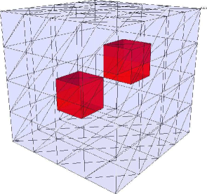
Figure 1. Geometry of the two material subdomains test problem.

We run a simple test problem on the unit cube, which is a model of a soft/hard material enclosure. As in [33], we only consider the two material subdomains case pictured in Figure 1, and we let $\Omega_{2}$ be the union of the two internal cubes, while $\Omega_{1}$ denotes the rest of the domain. The problem was discretized with linear finite elements on regular tetrahedral mesh, using zero Dirichlet boundary conditions on the boundary. The right-hand side in all the tests, was chosen to correspond to the unit constant function, and the initial guess was a vector of zeros. Some of the computed numerical solutions are plotted in Figure 2.

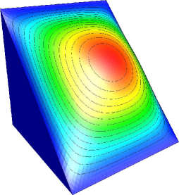
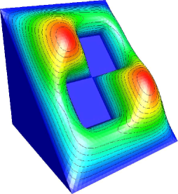
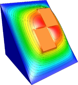
Figure 2. Approximate solutions in a cut inside the domain corresponding to $\omega=1$, $\rho=1$ (left); $\omega=1$, $\rho_{1}=1$, $\rho_{2}=10^{8}$ (center); and $\omega_{1}=1$, $\omega_{2}=10^{8}$, $\rho=1$ (right).

Since we can always rescale the original equation, we can assume, without a loss of generality, that $\omega_{2}=1$. In particular, when $\omega$ is a constant we will set it equal to one. This is the case that we set to explore first.

5.1. The case of constant $\omega$

To restrict the parameter range, we first set $\omega=1$ and allow $\rho_{1}$ and $\rho_{2}$ to vary independently in $\{0\}\cup[10^{-8},10^{8}]$. The results of Gauss-Seidel preconditioned conjugate gradient are presented in Table 1. Here $\ell$ denotes the refinement level corresponding to problem size $N$ and mesh size $h$. We also use the “scientific” notation 1e+p to denote the number $10^{p}$.

$\omega_{1}=1$		$\rho_{1}$
$\omega_{2}=1$		0	1e-8	1e-6	1e-4	1e-2	1e-0	1e+2	1e+4	1e+6	1e+8
$\ell=3$, $h^{2}\approx$ 1e-3, $N=35,937$
	0	62	62	62	62	62	66	50	20	19	19
	1e-8	62	62	62	62	62	66	50	20	19	19
	1e-6	62	62	62	62	62	66	50	20	19	19
	1e-4	62	62	62	62	62	66	50	20	19	19
	1e-2	62	62	62	62	62	66	50	20	19	19
$\rho_{2}$	1e-0	66	66	66	66	66	62	50	20	19	19
	1e+2	69	69	69	69	69	68	46	19	19	18
	1e+4	63	63	63	63	63	62	45	10	15	14
	1e+6	60	60	60	60	60	60	45	13	15	15
	1e+8	60	60	60	60	60	60	45	13	15	15
$\ell=4$, $h^{2}\approx$ 2.5e-4, $N=274,625$
	0	120	120	120	120	120	120	96	38	36	36
	1e-8	120	120	120	120	120	120	96	38	36	36
	1e-6	120	120	120	120	120	120	96	38	36	36
	1e-4	120	120	120	120	120	120	96	38	36	36
	1e-2	120	120	120	120	120	120	96	38	36	36
$\rho_{2}$	1e-0	121	121	121	121	121	120	96	38	36	36
	1e+2	133	133	133	133	133	132	85	37	35	35
	1e+4	123	123	123	123	123	122	89	13	14	15
	1e+6	117	117	117	117	117	116	89	14	14	15
	1e+8	117	117	117	117	117	117	89	14	15	15

Table 1. Number of GS-CG iterations when $\omega=1$.

Several things are apparent from Table 1. First, when $\rho h^{2}\gtrsim\omega$ (the lower right corner in the tables) the problem is well conditioned and GS-CG is an efficient solver. Second, the convergence is largely independent of the jumps in $\rho$ and the number of iterations is proportional to $h^{-1}$, as expected by Theorem 2.3. Finally, it is clear that the problem of hard enclosure, when $\rho_{2}>\rho_{1}$, is more difficult than the one of soft enclosure ($\rho_{1}>\rho_{2}$).

Motivated by the above observations, we choose to restrict our further experiments to the case $\omega=1$, $\rho_{1}=1$. This way the results have a more compact form, as can be seen by comparing Table 1 and Table 2.

		$\rho_{2}$
$\ell$	$N$	0	1e-8	1e-6	1e-4	1e-2	1e-0	1e+2	1e+4	1e+6	1e+8
1	729	18	18	18	18	18	18	18	16	16	16
2	4,913	36	36	36	36	36	36	38	34	34	34
3	35,937	66	66	66	66	66	62	68	62	60	60
4	274,625	120	120	120	120	120	120	132	122	116	117

Table 2. Number of GS-CG iterations when $\omega=1$ and $\rho_{1}=1$.

In Tables 3–5 we demonstrate the performance of the BPX preconditioner and the Multigrid solver and preconditioner on problems with constant $\omega$. The results indicate that BPX-CG may have a nearly-optimal convergence rate, see Theorem 4.9, while the convergence of Multigrid is optimal.

		$\rho_{2}$
$\ell$	$N$	0	1e-8	1e-6	1e-4	1e-2	1e-0	1e+2	1e+4	1e+6	1e+8
1	729	20	20	20	20	20	20	19	19	19	18
2	4,913	27	27	27	27	27	27	27	30	31	30
3	35,937	31	31	31	31	31	31	31	35	37	37
4	274,625	33	33	33	33	33	33	33	38	43	42
5	2,146,689	35	35	35	35	35	35	35	39	47	47

Table 3. Number of BPX-CG iterations when $\omega=1$ and $\rho_{1}=1$.

	$\rho_{2}$
$\ell$	0	1e-8	1e-6	1e-4	1e-2	1e-0	1e+2	1e+4	1e+6	1e+8
1	16 (0.17)	16 (0.17)	16 (0.17)	16 (0.17)	16 (0.17)	16 (0.17)	16 (0.16)	17 (0.16)	17 (0.17)	17 (0.17)
2	18 (0.20)	18 (0.20)	18 (0.20)	18 (0.20)	18 (0.20)	18 (0.20)	18 (0.20)	22 (0.27)	23 (0.28)	23 (0.28)
3	18 (0.21)	18 (0.21)	18 (0.21)	18 (0.21)	18 (0.21)	18 (0.21)	18 (0.21)	25 (0.32)	26 (0.32)	25 (0.32)
4	18 (0.21)	18 (0.21)	18 (0.21)	18 (0.21)	18 (0.21)	18 (0.21)	18 (0.21)	26 (0.33)	27 (0.35)	27 (0.35)
5	18 (0.21)	18 (0.21)	18 (0.21)	18 (0.21)	18 (0.21)	18 (0.21)	18 (0.21)	27 (0.34)	29 (0.38)	28 (0.37)

Table 4. Number of Multigrid iterations and asymptotic convergence factors when $\omega=1$ and $\rho_{1}=1$.

		$\rho_{2}$
$\ell$	$N$	0	1e-8	1e-6	1e-4	1e-2	1e-0	1e+2	1e+4	1e+6	1e+8
1	729	9	9	9	9	9	9	9	8	9	9
2	4,913	10	10	10	10	10	10	10	11	11	11
3	35,937	10	10	10	10	10	10	10	12	12	12
4	274,625	10	10	10	10	10	10	10	12	13	12
5	2,146,689	10	10	10	10	10	10	10	12	13	13

Table 5. Number of MG-CG iterations when $\omega=1$ and $\rho_{1}=1$.

5.2. The case of constant $\rho$

Next, we consider the case when the mass term coefficient is a constant. As in the previous section, we first perform a parameter study to determine an appropriate scaling of $\rho$ when $\omega_{2}$ is fixed to be one. The results are presented in Table 6, and in many respects are similar to those from Table 1. For example, the number of GS-GC iterations doubles from one level to the next, though the actual numbers are several times larger than those in Table 1.

		$\rho$
$\omega_{2}=1$		0	1e-8	1e-6	1e-4	1e-2	1e-0	1e+2	1e+4	1e+6	1e+8
$\ell=3$, $h^{2}\approx$ 1e-3, $N=35,937$
	1e-8	117	173	90	60	59	53	35	15	15	15
	1e-6	108	108	107	82	58	53	35	15	15	15
	1e-4	97	97	97	97	75	52	35	15	15	15
	1e-2	87	87	87	87	87	66	34	15	15	15
$\omega_{1}$	1e-0	62	62	62	62	62	62	46	10	15	15
	1e+2	74	74	74	74	74	74	73	48	12	15
	1e+4	68	68	68	68	68	68	68	69	48	12
	1e+6	63	63	63	63	63	63	63	64	69	48
	1e+8	59	59	59	59	59	59	60	59	65	69
$\ell=4$, $h^{2}\approx$ 2.5e-4, $N=274,625$
	1e-8	348	347	178	107	102	90	62	15	15	15
	1e-6	212	222	211	163	102	90	62	15	15	15
	1e-4	193	193	193	192	150	91	62	15	15	15
	1e-2	169	169	169	169	168	128	61	14	15	15
$\omega_{1}$	1e-0	120	120	120	120	120	120	85	13	14	15
	1e+2	141	141	141	141	141	141	140	94	13	15
	1e+4	132	132	132	132	132	132	132	132	94	14
	1e+6	124	124	124	124	124	124	124	123	132	94
	1e+8	113	113	113	113	113	113	113	112	123	132

Table 6. Number of GS-CG iterations when $\omega_{2}=1$ and $\rho$ is a constant.

Examining the results in Table 6, we can conclude that the most challenging problems occur when $\rho$ and $\omega_{1}$ are of the same magnitude. Therefore, we restrict the experiments in this section to the case $\omega_{2}=1$, $\rho=\omega_{1}$.

		$\omega_{1}$
$\ell$	$N$	1e-8	1e-6	1e-4	1e-2	1e-0	1e+2	1e+4	1e+6	1e+8
1	729	30	25	23	21	18	19	19	19	19
2	4,913	87	55	51	45	36	40	39	39	39
3	35,937	173	107	97	87	62	73	69	69	69
4	274,625	347	211	192	168	120	140	132	132	132

Table 7. Number of GS-CG iterations when $\omega_{2}=1$ and $\rho=\omega_{1}$.

The results for GS-CG are shown in Table 7. Clearly, the problem of hard enclosure, when $\omega_{1}$ is small, is much more challenging than the case of large $\omega_{1}$. In contrast to Table 2, the number of iterations increases significantly with the magnitude of the jump. This is due to the fact that the condition number is proportional to $\mathcal{J}(\omega)$, see Theorem 2.3 and the discussion after Theorem 2.1 in [33].

		$\omega_{1}$
$\ell$	$N$	1e-8	1e-6	1e-4	1e-2	1e-0	1e+2	1e+4	1e+6	1e+8
1	729	21	22	22	22	20	20	20	20	20
2	4,913	34	34	34	33	27	29	28	28	28
3	35,937	41	41	41	40	31	33	32	32	32
4	274,625	46	46	47	44	33	35	35	35	35
5	2,146,689	51	51	52	48	35	38	38	37	38

Table 8. Number of BPX-CG iterations when $\omega_{2}=1$ and $\rho=\omega_{1}$.

To a lesser extend, this trend is present in the results with BPX preconditioning reported in Table 8. Even though the increase in the number of iteration due to the jump in $\omega$ is not as large as for GS-CG, the influence of $\mathcal{J}(\omega)$ on the condition number can be observed if we plot the convergence history of the PCG iterations. Such a plot is presented in Figure 3, where one can clearly see that when $\omega_{1}=10^{-8}$, PCG needs several extra iterations to resolve the eigenvector corresponding to the isolated minimal eigenvalue, cf. Figure 3 in [33].

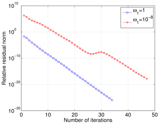
Figure 3. Convergence history for BPX-CG when $\omega_{2}=1$, $\rho=\omega_{1}$ and $\omega_{1}\in\{1,10^{-8}\}$. Problem size $N=274,625$.

	$\omega_{1}$
$\ell$	1e-4	1e-2	1e-0	1e+2	1e+4	1e+6	1e+8
1	41 (0.61)	38 (0.55)	16 (0.17)	18 (0.20)	18 (0.20)	18 (0.20)	18 (0.20)
2	100 (0.82)	69 (0.74)	18 (0.20)	20 (0.24)	20 (0.24)	19 (0.24)	19 (0.24)
3	216 (0.93)	100 (0.81)	18 (0.21)	21 (0.26)	21 (0.26)	21 (0.27)	21 (0.26)
4	440 (0.97)	124 (0.85)	18 (0.21)	22 (0.29)	22 (0.29)	22 (0.29)	22 (0.29)
5	843 (0.98)	140 (0.87)	18 (0.21)	23 (0.31)	23 (0.31)	23 (0.31)	23 (0.31)

Table 9. Number of Multigrid iterations and asymptotic convergence factors when $\omega_{2}=1$ and $\rho=\omega_{1}$.

In the previous section we observed that Multigrid has asymptotic convergence factor independent of the jumps in $\rho$ (see Table 4). This is no longer true when $\omega$ is not a constant, as demonstrated in Table 9. Indeed, the condition number of the Multigrid preconditioned system is bounded by $\min\{\mathcal{J}(\omega),h^{-1}\}$, so when the jump is large enough (as in the leftmost column) the iterations double with each refinement level.

		$\omega_{1}$
$\ell$	$N$	1e-8	1e-6	1e-4	1e-2	1e-0	1e+2	1e+4	1e+6	1e+8
1	729	10	10	10	10	9	9	9	9	9
2	4,913	13	13	13	13	10	11	11	11	11
3	35,937	14	14	14	14	10	11	11	11	11
4	274,625	15	15	15	15	10	11	11	11	11
5	2,146,689	16	16	16	15	10	12	12	12	12

Table 10. Number of MG-CG iterations when $\omega_{2}=1$ and $\rho=\omega_{1}$.

Using Multigrid as a preconditioner resolves this problem, since there are only finite number of small eigenvalues corresponding to the jump in $\omega$. The results in Table 10 demonstrate a nearly optimal convergence with respect to the mesh size.

5.3. The case of discontinuous $\omega$ and $\rho$

In this section we present a numerical investigation of the general case when both $\omega$ and $\rho$ are discontinuous. Note that the theory developed in this paper can be applied only if we can construct an interpolation operator which is stable in both the $\rho$-weighted and the $\omega$-weighted $L^{2}$-inner products. This is the case, for example if $\omega_{1}\leq\omega_{2}$ and $\rho_{1}\leq\rho_{2}$.

		$\omega_{1}/\omega_{2}$
		1e-8	1e-6	1e-4	1e-2	1e-0	1e+2	1e+4	1e+6	1e+8
	1e-8	169	170	170	164	133	141	139	139	113
	1e-6	193	194	191	169	133	141	139	139	113
	1e-4	214	209	193	169	133	141	139	139	113
	1e-2	344	213	193	169	132	141	138	138	122
$\rho_{1}/\rho_{2}$	1e-0	347	222	193	169	120	141	132	132	132
	1e+2	268	221	193	169	120	141	132	124	133
	1e+4	111	164	192	169	120	141	132	124	133
	1e+6	108	104	151	168	120	141	132	124	133
	1e+8	101	101	100	131	120	141	132	124	132

Table 11. Number of GS-CG iterations when $\omega_{2}=1$, while $\omega_{1}$, $\rho_{1}$ and $\rho_{2}$ are allowed to vary. Each cell in the table represents a maximum over a range of values for $\rho$. Problem size $N=274,625$.

In Table 11 we show the results of a parameter study based on Gauss-Seidel preconditioning. We emphasize that each cell in this table represents a maximum over several possible values for $\rho$, which result in a jump of the same magnitude $\rho_{1}/\rho_{2}$. Clearly, the difficulty of the problem is determined mostly by the jump in $\omega$, so we choose to concentrate on the most challenging case $\omega_{1}=10^{-8}.$

The results of using for BPX and Multigrid V-cycle preconditioners for this choice of $\omega$ are shown in Table 12 and Table 13 respectively. They indicate that when $\rho_{1}\leq\rho_{2}$, the PCG behavior is generally similar to the case when $\rho$ is a constant. This is not surprising, since as we mentioned earlier, our convergence theory can be applied in this special case. When $\rho_{1}>\rho_{2}$, the convergence deteriorates, though not significantly.

		$\rho_{1}/\rho_{2}$
$\ell$	$N$	1e-8	1e-6	1e-4	1e-2	1e-0	1e+2	1e+4	1e+6	1e+8
1	729	20	20	20	21	21	21	21	21	21
2	4,913	32	33	33	33	34	32	32	32	32
3	35,937	39	40	40	40	41	42	42	42	42
4	274,625	44	45	45	46	46	48	49	49	49

Table 12. Number of BPX-CG iterations when $\omega_{1}=10^{-8}$ and $\omega_{2}=1$. Each cell in the table represents a maximum over a range of values for $\rho$.

		$\rho_{1}/\rho_{2}$
$\ell$	$N$	1e-8	1e-6	1e-4	1e-2	1e-0	1e+2	1e+4	1e+6	1e+8
1	729	10	10	10	10	10	10	10	10	10
2	4,913	13	13	13	13	13	13	13	13	13
3	35,937	14	14	14	14	14	15	15	15	15
4	274,625	14	15	15	15	15	17	17	17	17

Table 13. Number of MG-CG iterations when $\omega_{1}=10^{-8}$ and $\omega_{2}=1$. Each cell in the table represents a maximum over a range of values for $\rho$.

To further investigate the effect of adding jumps in $\rho$, when $\omega$ is already discontinuous we consider a test problem in two dimensions. We start with the coarse triangulation shown in Figure 4 and randomly assign each coarse triangle to one of two possible subdomains. The mesh is then refined $\ell$ times.

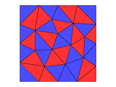
Figure 4. Coarse triangulation ($\ell=0$) and the two material subdomains for the two-dimensional test problem.

We focus on the case $\omega_{1}=10^{-8}$ and $\omega_{2}=1$ and allow $\rho_{1}$ and $\rho_{2}$ to vary as in the previous experiments. The results for BPX and Multigrid preconditioners are shown in Table 14 and Table 15. They appear to indicate that adding jumps in $\rho$ can lead to a significant deterioration in the convergence of this problem. The approximate solution corresponding to one of the most challenging cases is plotted in Figure 5.

		$\rho_{1}/\rho_{2}$
$\ell$	$N$	1e-8	1e-6	1e-4	1e-2	1e-0	1e+2	1e+4	1e+6	1e+8
4	4,737	49	50	51	53	56	63	64	64	64
5	18,689	57	58	59	62	66	78	79	79	79
6	74,241	63	67	67	74	77	93	95	95	95
7	295,937	73	76	76	87	93	109	122	123	123
8	1,181,697	81	83	83	100	110	125	164	164	164
9	4,722,689	88	90	90	114	127	141	209	211	211

Table 14. Two-dimensional test problem: Number of BPX-CG iterations when $\omega_{1}=10^{-8}$ and $\omega_{2}=1$. Each cell in the table represents a maximum over a range of values for $\rho$.

		$\rho_{1}/\rho_{2}$
$\ell$	$N$	1e-8	1e-6	1e-4	1e-2	1e-0	1e+2	1e+4	1e+6	1e+8
4	4,737	18	18	18	19	20	23	23	23	23
5	18,689	19	21	21	21	22	26	26	26	26
6	74,241	21	23	23	23	25	29	30	30	30
7	295,937	23	25	25	25	27	32	40	40	40
8	1,181,697	26	26	26	27	30	36	52	53	53
9	4,722,689	28	28	28	30	32	40	65	66	66

Table 15. Two-dimensional test problem: Number of MG-CG iterations when $\omega_{1}=10^{-8}$ and $\omega_{2}=1$. Each cell in the table represents a maximum over a range of values for $\rho$.

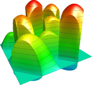
Figure 5. Approximate solutions corresponding to $\omega_{1}=10^{-8}$, $\omega_{2}=1$, $\rho_{1}=10^{4}$ and $\rho_{2}=1$.

References

- [1] B. Aksoylu, I. Graham, H. Klie, and R. Scheichl. Towards a rigorously justified algebraic preconditioner for high-contrast diffusion problems. Computing and Visualization in Science, 11(4):319–331, 2008.
- [2] O. Axelsson. Iterative solution methods. Cambridge University Press, Cambridge, 1994.
- [3] O. Axelsson. Iteration number for the conjugate gradient method. Mathematics and Computers in Simulation, 61(3-6):421–435, 2003. MODELING 2001 (Pilsen).
- [4] B. Ayuso de Dios, M. Holst, Y. Zhu, and L. Zikatanov. Multilevel preconditioners for discontinuous, Galerkin approximations of elliptic problems, with jump coefficients. Math. Comp., 83(287):1083–1120, 2014.
- [5] J. H. Bramble, J. E. Pasciak, and J. Xu. Parallel multilevel preconditioners. Mathematics of Computation, 55(191):1–22, 1990.
- [6] J. H. Bramble and J. Xu. Some estimates for a weighted projection. Mathematics of Computation, 56:463–476, 1991.
- [7] T. F. Chan and W. L. Wan. Robust multigrid methods for nonsmooth coefficient elliptic linear systems. Journal of Computational and Applied Mathematics, 123(1-2):323–352, 2000.
- [8] L. Chen, M. Holst, J. Xu, and Y. Zhu. Local multilevel preconditioners for elliptic equations with jump coefficients on bisection grids. Computing and Visualization in Science, 15(5):271–289, 2012.
- [9] S. Cho, S. V. Nepomnyaschikh, and E.-J. Park. Domain decomposition preconditioning for elliptic problems with jumps in coefficients. Technical Report RICAM-Report 05-22, Johann Radon Institute for Computational and Applied Mathematics, Austrian Academy of Sciences, Linz, 2005.
- [10] M. Dryja, M. V. Sarkis, and O. B. Widlund. Multilevel Schwarz methods for elliptic problems with discontinuous coefficients in three dimensions. Numerische Mathematik, 72(3):313–348, 1996.
- [11] J. Galvis and Y. Efendiev. Domain decomposition preconditioners for multiscale flows in high-contrast media. Multiscale Modeling & Simulation, 8(4):1461–1483, 2010.
- [12] G. H. Golub and C. F. Van Loan. Matrix computations. Johns Hopkins Studies in the Mathematical Sciences. Johns Hopkins University Press, Baltimore, MD, third edition, 1996.
- [13] I. Graham, P. Lechner, and R. Scheichl. Domain decomposition for multiscale PDEs. Numerische Mathematik, 106(4):589–626, June 2007.
- [14] I. G. Graham and M. J. Hagger. Unstructured additive Schwarz-conjugate gradient method for elliptic problems with highly discontinuous coefficients. SIAM Journal on Scientific Computing, 20:2041–2066, 1999.
- [15] W. Hackbusch. Multigrid Methods and Applications, volume 4 of Computational Mathematics. Springer–Verlag, Berlin, 1985.
- [16] W. Hackbusch. Iterative Solution of Large Sparse Systems of Equations, volume 95 of Applied Mathematical Sciences. Springer-Verlag New York, Inc., 1994.
- [17] R. Hiptmair and J. Xu. Nodal auxiliary space preconditioning in H(curl) and H(div) spaces. SIAM Journal on Numerical Analysis, 45:2483–2509, 2007.
- [18] Tz. Kolev and P. Vassilevski. Parallel auxiliary space AMG for H(curl) problems. J. Comput. Math., 27:604–623, 2009. Special issue on Adaptive and Multilevel Methods in Electromagnetics.
- [19] J. Kraus and M. Wolfmayr. On the robustness and optimality of algebraic multilevel methods for reaction–diffusion type problems. Computing and Visualization in Science, 16(1):15–32, 2013.
- [20] MFEM: Modular parallel finite element methods library. http://mfem.googlecode.com.
- [21] R. Nabben and C. Vuik. A comparison of deflation and coarse grid correction applied to porous media flow. SIAM Journal on Numerical Analysis, 42(4):1631–1647, 2004.
- [22] P. Oswald. On the robustness of the BPX-preconditioner with respect to jumps in the coefficients. Mathematics of Computation, 68:633–650, 1999.
- [23] M. Petzoldt. A posteriori error estimators for elliptic equations with discontinuous coefficients. Advances in Computational Mathematics, 16(1):47–75, 2002.
- [24] R. Scheichl and E. Vainikko. Additive Schwarz with aggregation-based coarsening for elliptic problems with highly variable coefficients. Computing, 80(4):319–343, Sept. 2007.
- [25] R. Scheichl, P. Vassilevski, and L. Zikatanov. Multilevel methods for elliptic problems with highly varying coefficients on nonaligned coarse grids. SIAM Journal on Numerical Analysis, 50(3):1675–1694, 2012.
- [26] R. Scott and S. Zhang. Finite element interpolation of nonsmooth functions satisfying boundary conditions. Mathematics of Computation, 54:483–493, 1990.
- [27] P. Vassilevski. Multilevel block factorization preconditioners: Matrix-based analysis and algorithms for solving finite element equations. Springer, 2008.
- [28] J. Wang. New convergence estimates for multilevel algorithms for finite-element approximations. Journal of Computational and Applied Mathematics, 50:593–604, 1994.
- [29] J. Wang and R. Xie. Domain decomposition for elliptic problems with large jumps in coefficients. In the Proceedings of Conference on Scientific and Engineering Computing, pages 74–86. National Defense Industry Press, 1994.
- [30] O. B. Widlund. Some Schwarz methods for symmetric and nonsymmetric elliptic problems. In D. E. Keyes, T. F. Chan, G. A. Meurant, J. S. Scroggs, and R. G. Voigt, editors, Fifth International Symposium on Domain Decomposition Methods for Partial Differential Equations, pages 19–36, Philadelphia, 1992. SIAM.
- [31] J. Xu. Iterative methods by space decomposition and subspace correction. SIAM Review, 34:581–613, 1992.
- [32] J. Xu. A new class of iterative methods for nonselfadjoint or indefinite problems. SIAM Journal on Numerical Analysis, 29:303–319, 1992.
- [33] J. Xu and Y. Zhu. Uniform convergent multigrid methods for elliptic problems with strongly discontinuous coefficients. Mathematical Models and Methods in Applied Science, 18(1):77 –105, 2008.
- [34] J. Xu and L. Zikatanov. The method of alternating projections and the method of subspace corrections in Hilbert space. Journal of The American Mathematical Society, 15:573–597, 2002.
- [35] Y. Zhu. Domain decomposition preconditioners for elliptic equations with jump coefficients. Numerical Linear Algebra with Applications, 15(2-3):271–289, 2008.
- [36] Y. Zhu. Analysis of a multigrid preconditioner for Crouzeix-Raviart discretization of elliptic partial differential equation with jump coefficients. Numer. Linear Algebra Appl., 21(1):24–38, 2014.