Random center vortex lines in continuous 3D space-time

Abstract

We present a model of center vortices, represented by closed random lines in continuous 2+1- dimensional space-time. These random lines are modeled as being piece-wise linear and an ensemble is generated by Monte Carlo methods. The physical space in which the vortex lines are defined is a cuboid with periodic boundary conditions. Besides moving, growing and shrinking of the vortex configuration, also reconnections are allowed. Our ensemble therefore contains not a fixed, but a variable number of closed vortex lines. This is expected to be important for realizing the deconfining phase transition. Using the model, we study both vortex percolation and the potential $V(R)$ between quark and anti-quark as a function of distance $R$ at different vortex densities, vortex segment lengths, reconnection conditions and at different temperatures. We have found three deconfinement phase transitions, as a function of density, as a function of vortex segment length, and as a function of temperature. The model reproduces the qualitative features of confinement physics seen in $SU(2)$ Yang-Mills theory.

1 Introduction

In $D$-dimensional space-time, center vortices are (thickened) ($D-2$)-dimensional chromo-magnetic flux degrees of freedom. The center vortex picture of the confining vacuum ’t Hooft (1978); Yoneya (1978); Mack and Petkova (1979); Nielsen and Olesen (1979) assumes that these are the relevant degrees of freedom in the infrared sector of the strong interaction; the center vortices consequently are taken to be weakly coupled and can thus be expected to behave as random lines (for $D=3$) or random surfaces (for $D=4$). The magnetic flux carried by the vortices is quantized in units which are singled out by the topology of the gauge group, such that the flux is stable against small local fluctuations of the gauge fields. The vortex model of confinement states that the deconfinement transition is simply a percolation transition of these chromo-magnetic flux degrees of freedom. It is theoretically appealing and was confirmed by a multitude of numerical calculations, both in lattice Yang-Mills theory and within a corresponding infrared effective model, see Greensite (2003) for an overview. Lattice simulations further indicate that vortices may also be responsible for topological charge and $\chi$SB de Forcrand and D’Elia (1999); Alexandrou et al. (2000); Engelhardt (2002); V. Bornyakov et al. (2008); R. Höllwieser, M. Faber, J. Greensite, U.M. Heller, and Š. Olejník (2008); R. Höllwieser, M. Faber, U.M. Heller (2011); R. Höllwieser, T. Schweigler, M. Faber and U.M. Heller (2013), and thus unify all non-perturbative phenomena in a common framework.

We introduce a model of random flux lines in $D=2+1$ space-time dimensions. The lines are composed of straight segments connecting nodes randomly distributed in three-dimensional space. Allowance is made for nodes moving as well as being added or deleted from the configurations during Monte Carlo updates. Furthermore, Monte Carlo updates disconnecting and fusing vortex lines, i.e. reconnection updates were implemented. Given that the deconfining phase transition is a percolation transition, such processes play a crucial role in the vortex picture. The model has been formulated in a finite volume, with periodic boundary conditions, which will allow for a study of finite temperatures (via changes in the temporal extent of the volume). The resulting vortex ensemble will be used, in particular, to measure the string tension and its behavior as a function of temperature, with a view towards detecting the high-temperature deconfining phase transition.

2 The Model

The physical space in which the vortex lines are defined is a cuboid $L_{S}^{2}\times L_{T}$ with ”spatial” extent $L_{S}$, ”temporal” extent $L_{T}$ and periodic boundary conditions in all directions. The random lines are modeled as being piece-wise linear between nodes, with vortex length $L$ between two nodes restricted to a certain range $L_{min}<L<L_{max}$. This range in some sense sets the scale of the model; for practical reasons we choose a scale of $L\approx 1$, i.e. $L_{min}=0.3$ and $L_{max}=1.7$ in these dimensionless units. Within this paper we use volumes with $L_{S}=16$, where finite size effects are under control, and varying time lengths $L_{T}$. The variation of the vortex lengths range will also be examined. An ensemble is generated by Monte Carlo methods, starting with a random initial configuration. A Metropolis algorithm is applied to all updates using the action $S=\alpha L+\gamma\varphi^{2},$ with action parameters $\alpha$ and $\gamma$ for the vortex length $L$ and the vortex angle $\varphi$ between two adjacent segments respectively. At a given (current) node the vortex length $L$ is defined to be the distance to the previous node and the vortex angle is the angle between the oriented vectors of the vortex lines connecting the previous, current and next nodes. When two vortices approach each other, they can reconnect or separate at a bottleneck. The ensemble therefore will contain not a fixed, but a variable number of closed vortex lines or ”vortex clusters”. This is expected to be important for realizing the deconfining phase transition.

Move, add and delete updates are applied to the vortex nodes via the Metropolis algorithm, i.e. the difference of the action of the affected nodes before and after the update determines the probability of the update to be accepted. The move update moves the current node by a random vector of maximal length $r_{m}=4L_{min}$, it affects the action of three nodes, the node itself and its neighbors. The add update adds a node at a random position within a radius $r_{a}=3L_{min}$ around the midpoint between the current and the next node. The action before the update is given by the sum of the action at the current and the next node, while the action after the update is the sum of the action at the current, the new and the next node. Deleting the current node, on the other hand, affects three nodes before the update and only two nodes after the update. Therefore the probability for the add update is in general much smaller than for the delete update and the vortex structure would soon vanish if both updates were tried equally often. Hence, the update strategy is randomized to move a node in two out of three cases ($66\%$), and apply the add update about five times more often than the delete update ($28\%$ vs. $6\%$). If the current node is not deleted, all nodes around the current node are considered for reconnections. The reconnection update causes the cancellation of two close, nearly parallel vortex lines and reconnection of the involved nodes with new vortex lines. The reconnection update is also subjected to the Metropolis algorithm, considering the action of the four nodes involved. All updates resulting in vortex lengths $L$ out of the range $L_{min}<L<L_{max}$ are rejected. Finally, a density parameter $d$ is introduced, restricting the number of nodes in a certain volume. The add update is rejected if the number of nodes within a $3\times 3\times 3$ volume around the new node exceeds the density parameter $d$.

3 Measurements and Observables

For our simulations we start random vortex line configurations and do $10^{4}$ thermalization sweeps through the whole configuration, i.e. updating all single nodes within each sweep. After that $2-5*10^{5}$ measurements of the average action per node, the actual density, average vortex length and angle and Wilson loops were measured and a vortex cluster analysis was performed every $n_{s}=10$ Monte Carlo sweeps. The vortex cluster routine counts the number of closed vortex clusters, the number of vortex nodes/lines for each cluster, the cluster size or maximal extent of each cluster and the number of clusters winding around the time dimension. Taking into account the periodic boundary conditions, the maximal cluster size is given by $s_{m}=L_{S}^{2}/2+L_{T}^{2}/4$. The Wilson loop $W(R,T)$ is a common observable in lattice gauge field theory. It is a closed (rectangular) loop in space and time and can be interpreted as the creation of a quark–anti-quark pair with a certain spatial separation $R$ evolving for some time $T$ and annihilating again. In our continuous space model we are not restricted to rectangular loops, but they are more convenient for actual calculations. The Wilson loop is calculated by counting the number $n_{p}$ of vortex lines piercing through a plane of extent $R\times T$, resulting in $W(R,T)=(-1)^{n_{p}}$. The expectation values of the time-like Wilson loops $\langle W(R,T)\rangle$ give the quark–anti-quark potential $V(R)\propto-\underset{T\rightarrow\infty}{lim}\;log\langle W(R,T)\rangle/T$. To extract the string tension $\sigma$ of the system an ansatz $V(R)=\sigma R+C/R+V_{0}$ is fitted to the potentials. The spatial string tension $\sigma_{s}$ is obtained from spatial Wilson loops.

4 Results and Discussion

In Fig. 1 we show the the potential $V(r)$ between quark and anti-quark and the string tension $\sigma$ as well as the maximal cluster size as a function of inverse temperature $L_{T}$ and density cutoff $d$. We observe a phase transition as a function of the inverse temperature $L_{T}$. The quark–anti-quark potential shown in Fig. 1a is still flat (asymptotically) for $L_{T}=4$ while we may see some linearly rising behavior for $L_{T}=9$. In between the potentials do not show an exactly linear behavior, and the determination of the string tension is somewhat ambiguous, but the bending is of course caused by the finite spatial extent of the physical volume. In the $d=4$ case there is no sharp but a rather smooth transition, which is caused by the small density cutoff. The transition gets sharper and the transition temperature increases with the density cutoff $d$. We locate the phase transition for $d=6$ between $L_{T}=2-4$, for $d=8$ between $L_{T}=1.6-2.5$, for $d=10$ between $L_{T}=1.5-2$ and for $d=12$ between $L_{T}=1.2-1.5$. Further, we notice that Fig. 1b and d show a perfect agreement between confinement (string tension) and percolation (maximal cluster size) transition.

a) b)

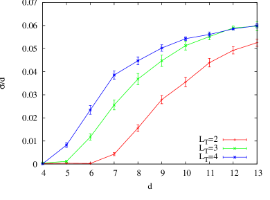
c) d)

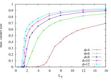
Figure 1: Results for $16^{2}\times L_{T}$ volumes with vortex lengths $L_{max}=1.7$ and $L_{min}=0.3$: a) Quark–anti-quark potentials for density cutoff $d=4$, b) string tension $\sigma$ and d) maximum cluster size vs. time extent $L_{T}$, note the good correlation between the two, and c) string tension $\sigma/d$ vs. density cutoff $d$.

In Fig. 1c we show the string tensions $\sigma/d$ for different density cutoffs $d=4-13$ for three different physical volumes $16^{2}\times L_{T}$ with $L_{T}=2-4$, $L_{max}=1.7$ and $L_{min}=0.3$. We observe a confinement phase transition with respect to the vortex density cutoff $d$. At $d=4$ all configurations are in the deconfined phase, the $L_{T}=4$ configurations immediately start to confine with increasing $d$, whereas $L_{T}=3$ and $L_{T}=2$ configurations start the phase transition at $d=5$ and $d=6$, respectively.

Another phase transition is observed for different maximal vortex segment lengths $L_{max}=1.0-2.2$ for a physical volume $16^{2}\times 2$ and a density cutoff $d=8$, with $L_{min}=0.3$. In Fig. 2a we show the string tensions $\sigma$ and $\sigma_{s}$ as well as maximal cluster size versus the different vortex lengths $L_{max}$. We observe a well defined phase transition starting at $L_{max}=1.5$, with no percolation and string tension $\sigma$ below that threshold and percolation resp. confinement above. Restricting the vortex line length to small values leads to small, separated vortex clusters which cannot reconnect or percolate and confinement is lost.

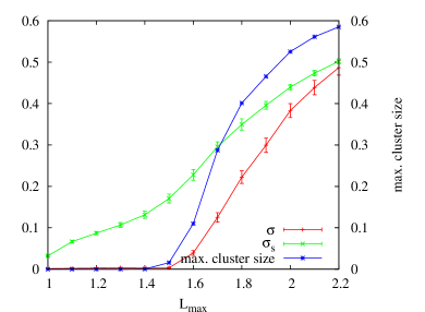
a) c)

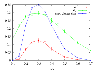
Figure 2: String tensions $\sigma$, $\sigma_{s}$ and maximal cluster size for $16^{2}\times 2$ volumes and density cutoff $d=8$ vs. vortex lengths a) $L_{max}$ and b) $L_{min}$.

The interpretation of the phase space with respect to the minimal vortex length $L_{min}$ is going to be more complex than in all other cases, since $L_{min}$ defines some sort of minimal length scale and we use it to restrict the minimal length of a vortex segment itself, the move radius $r_{m}=4L_{min}$, the add radius $r_{a}=3L_{min}$ and the reconnection length $r_{r}=L_{min}$. That means that if we choose a small $L_{min}$, the vortex clusters will not spread out very fast and reconnections are strongly suppressed. On the other hand a large $L_{min}$ will lead to large random fluctuations and a huge number of random recombinations leading to a very chaotic system. Both cases do not seem to realize the physical systems we want to study and our test configurations in $16^{2}\times 2$ volumes with vortex density $d=8$, maximal vortex length $L_{max}=1.7$ and varying $L_{min}$ seem to confirm these expectations. This setup happens to lie exactly at the critical value for the parameters of all the above mentioned phase transitions, i.e. finite temperature, vortex density and maximal vortex length $L_{max}$. In Fig. 2b we plot the string tensions $\sigma$, $\sigma_{s}$ and maximal cluster size versus $L_{min}=0.1-0.7$ in steps of $0.05$. We note deconfined phases for both, small and large $L_{min}$, on the one hand because of rather static and on the other hand because of very chaotic configurations, which both do not seem to show good percolation properties. At $L_{min}=0.3$ however, we find a common maximum for string tensions, maximal cluster size and average vortex density and simultaneously the average action shows a minimum. This finally motivates our initial choice for $L_{min}=0.3$, which seems to give rather stable configurations which allowed reliable studies of the above phase transitions.

In Fig. 3 we show sample configurations for various temperatures and density cutoff $d=4$. While for $L_{T}=2$ and $4$ (Fig. 3a and b) we see many small vortex clusters, we observe already one big cluster extending over the whole physical volume together with some small clusters for $L_{T}=8$ (Fig. 3c) while for $L_{T}=16$ (zero temperature, Fig. 3d) it seems as if almost all nodes were connected, representing the percolation property.

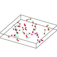
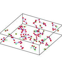
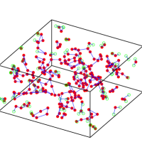
a) b) c) d)

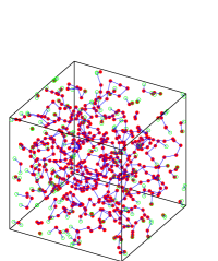
Figure 3: $16^{2}\times$ a) $2$, b) $4$, c) $8$ and d) $16$ configurations, density cutoff $d=4$, vortex lengths $L_{max}=1.7,L_{min}=0.3$.

5 Conclusions and Outlook

We introduced a $2+1$ dimensional center vortex model of the Yang-Mills vacuum. The vortices are represented by closed random lines which are modeled as being piece-wise linear and an ensemble is generated by Monte Carlo methods. The physical space in which the vortex lines are defined is a cuboid with periodic boundary conditions. The idea was to simulate continuous space-time, hence in contrast to existing discrete vortex models, the vortices are allowed to move freely and we have translational and rotational symmetry in our system. We further let vortex configurations grow and shrink and also reconnections are allowed, i.e. vortex lines may fuse or disconnect. Our ensemble therefore contains not a fixed, but a variable number of closed vortex lines. The reconnections are in fact the important ingredient for modeling a percolating system which is supposed to drive the confinement phase transition. All updates (move, add, delete, reconnect) are subjected to a Metropolis algorithm driven by an action depending on vortex segment length and the angle between two vortex segments, i.e. a length and curvature part. After fine-tuning all necessary parameters, we use the model to study both vortex percolation and the potential $V(R)$ between quark and anti-quark as a function of distance $R$ at different vortex densities, vortex segment lengths, reconnection conditions and at different temperatures (by varying the temporal extent of the physical volume).

We have found three confinement phase transitions, as a function of density, as a function of vortex segment length, and as a function of temperature. The confinement phase transitions are in perfect agreement with the percolation properties of the vortex configuration. For small vortex densities and vortex segment lengths the configuration consists of small, independent vortex clusters and for high temperatures vortex clusters prefer to wind around the (short) temporal extent of the volume and therefore these configurations are not percolating. The quark–anti-quark potentials in this case show no linearly rising behavior, i.e. no string tension is measured and the system is in the deconfined phase. Once we allow higher vortex densities, longer vortex segment lengths or temporal extent, i.e. lower temperature, the vortex configurations start to percolate and small clusters reconnect to mainly one big vortex cluster filling the whole volume. In this regime we measure a finite string tension, i.e. linearly rising quark–anti-quark potentials, hence the vortices confine quarks and anti-quarks. We also study the influence of reconnection parameters, which are obviously very crucial for the percolation properties. These parameters have to be fine-tuned very carefully in order to find the above phase transitions.

We plan the expansion of the model to four dimensions, where some sort of random triangulation of vortex surfaces is needed, which then allows to study topological properties in addition to the confinement transition. The complex parameter space of the three dimensional case definitely indicates the difficulty of this task, but still, the model constructed in this paper certainly reproduces the qualitative features of confinement physics seen in $SU(2)$ Yang-Mills theory.

References

- ’t Hooft (1978) G. ’t Hooft, Nucl. Phys. B138, 1 (1978).
- Yoneya (1978) T. Yoneya, Nucl. Phys. B144, 195 (1978).
- Mack and Petkova (1979) G. Mack, and V. B. Petkova, Ann. Phys. 123, 442 (1979).
- Nielsen and Olesen (1979) H. B. Nielsen, and P. Olesen, Nucl. Phys. B160, 380 (1979).
- Greensite (2003) J. Greensite, Prog. Part. Nucl. Phys. 51, 1 (2003), hep-lat/0301023.
- de Forcrand and D’Elia (1999) P. de Forcrand, and M. D’Elia, Phys. Rev. Lett. 82, 4582–4585 (1999), hep-lat/9901020.
- Alexandrou et al. (2000) C. Alexandrou, P. de Forcrand, and M. D’Elia, Nucl. Phys. A663, 1031–1034 (2000), hep-lat/9909005.
- Engelhardt (2002) M. Engelhardt, Nucl.Phys. B638, 81–110 (2002), hep-lat/0204002.
- V. Bornyakov et al. (2008) V. Bornyakov et al., Phys. Rev. D 77, 074507 (2008), 0708.3335.
- R. Höllwieser, M. Faber, J. Greensite, U.M. Heller, and Š. Olejník (2008) R. Höllwieser, M. Faber, J. Greensite, U.M. Heller, and Š. Olejník, Phys. Rev. D 78, 054508 (2008), 0805.1846.
- R. Höllwieser, M. Faber, U.M. Heller (2011) R. Höllwieser, M. Faber, U.M. Heller, JHEP 1106, 052 (2011), 1103.2669.
- R. Höllwieser, T. Schweigler, M. Faber and U.M. Heller (2013) R. Höllwieser, T. Schweigler, M. Faber and U.M. Heller, Phys.Rev. D88, 114505 (2013), 1304.1277.