The dilute Temperley–Lieb O($n=1$) loop model on a semi infinite strip: the ground state

Abstract

We consider the integrable dilute Temperley–Lieb (dTL) O($n=1$) loop model on a semi-infinite strip of finite width $L$. In the analogy with the Temperley–Lieb (TL) O($n=1$) loop model the ground state eigenvector of the transfer matrix is studied by means of a set of $q$-difference equations, sometimes called the $q$KZ equations. We compute some ground state components of the transfer matrix of the dTL model, and show that all ground state components can be recovered for arbitrary $L$ using the $q$KZ equation and certain recurrence relation. The computations are done for generic open boundary conditions.

1 Introduction

In the last decade the integrable loop models with the loop weight $n=1$ became a subject of great interest due to their relation to combinatorics, algebraic geometry, percolation, etc. Probably, the most striking result is the Razumov–Stroganov (RS) conjecture, relating the components of the ground state of the Temperley-Lieb (TL) loop model to alternating sign matrices [1, 25]. The weaker version of this conjecture [1] was proved in [12], while the stronger RS conjecture [25] in [4]. The ground state of the TL loop model is known to be related to certain orbital varieties. Namely, the entries of the ground state of the TL loop model coincide with the multidegrees of certain matrix varieties [12, 17]. The TL loop model at $n=1$ is equivalent to critical bond percolation. Studying the ground state of the TL model with different boundary conditions allows to compute some correlation functions for critical bond percolation [19, 18]. Since the O($1$) TL loop model appears to be very fruitful it motivates us to study also the dilute Temperley-Lieb (dTL) loop model [21, 23].

The dilute Temperley-Lieb (dTL) loop model, with loop weight $n=1$, is a formulation of critical site percolation. Hence, its ground state contains the information of certain correlation functions for critical site percolation. At $n=0$ the ground state of the dTL model may provide a method to approach the closed self avoiding walk in 2D. In both cases ($n=1$ and $n=0$) the scaling limits are described by a Schramm–Loewner evolution (SLE). It is, however, a conjecture for the self avoiding walk. The dTL loop model at finite size may provide insights to the relations to SLE.

We organize the paper as follows. In Section 2 we present the definitions and the basic ingredients. In Section 3 we set the loop weight to $1$ and study the $q$KZ equations, after we discuss the recurrence in size and finally compute the ground state. Discussions follow in Section 4. The explicit results for $\Psi_{L}$ for $L=1$ and $2$ are given in Appendix A. The discussion of the recurrence relation is presented in Appendix B .

2 The dilute O$(n)$ loop model

The loop model we discuss here is defined on the square lattice with finite width and infinite length. This domain can be seen as a half infinite strip that has two vertical half infinite boundaries and one finite horizontal boundary of length $L$. If we identify the vertical boundaries, and otherwise leave them free, this will lead to periodic boundary conditions. Here we do not identify the vertical boundaries, but allow there any configuration, leading to open boundary conditions. The configurations of the dTL model are collections of non-intersecting paths over the edges of the lattice. The paths are either closed, hence loops, or terminate on one of the boundaries. Classes of configurations can be labelled by the connectivities of the links on the horizontal boundary. Each edge of the horizontal boundary can be in two states: occupied or unoccupied. An occupied edge is connected to another edge on the horizontal boundary. This way each configuration of the model corresponds to a link pattern on the horizontal boundary. All link patterns form a vector space lp_L, thus the states of the model can be expressed in this vector space. An important idea that has led to many advances for the TL model is to consider more general lattices, i.e. lattices with distortions or inhomogeneities $z_{1},..,z_{L}$. When the loop weight is equal to $1$, the ground state configuration $\Psi_{L}$ becomes a vector with entries polynomial in $z_{i}$ satisfying certain $q$-difference equations, sometimes referred to as the quantum Knizhnik–Zamolodchikov equations ($q$KZ). A crucial ingredient for the computations is the conjectural expression for a certain entry of the ground state. Using this conjecture all other elements follow from the $q$KZ equations. This was the basis of the algorithm for the computation of the ground state components and the sum rules for the TL O$(1)$ loop models with various boundary conditions [12, 11, 28, 7, 3] and for the dTL O($1$) model with periodic boundary conditions [10]. We extend these results to the dTL O($1$) model with open boundary conditions.

2.1 Link pattern basis and the $R$-matrix

Consider the dilute O$(n)$ loop model on the square lattice on a semi-infinite strip. An example of a configuration of the model is given in Fig. 1.

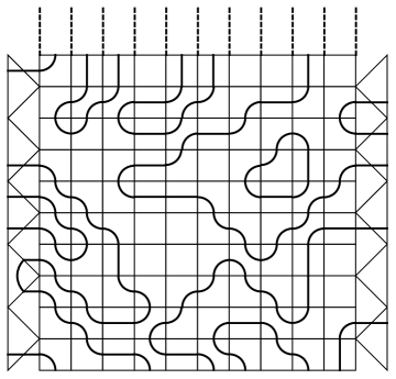
Figure 1: A typical configuration of the dilute O$(n)$ loop model on a fragment of a semi-infinite strip.

The paths can end at the horizontal boundary and two vertical boundaries. We classify all configurations according to their connectivity on the horizontal boundary, such a connectivity is called a link pattern. More precisely, let us label the edges of the lower boundary with numbers $1,2,..,L$ from left to right. If a path ends at an edge $i$, then this edge is said to be occupied, otherwise the edge is unoccupied. Moreover, we will distinguish the occupied edges connected with other edges on their left and on their right. It is convenient to label the connectivity by the variables $n_{i}$ for each edge $i$ which take the values $0$, $-1$ or $1$. In a given configuration we assign the label $n_{i}=0$ to an unoccupied edge $i$. We associate $n_{i}=1$ ($n_{i}=-1$) to an edge $i$ occupied and connected to an edge or a boundary on its right (left). With this notation the connectivity of a configuration is a sequence $\{n_{1},n_{2},..,n_{L}\}$. For example, the configuration depicted in Fig. 1 has the connectivity $\{-1,0,0,-1,0,1,1,0,-1,1\}$. We can represent this pictorially as in Fig. 2, where the vertical boundaries are represented by the leftmost and the rightmost points separated by a dashed line from the actual extremal edges of the horizontal boundary. The set of all link patterns, denoted by lp_L, is the basis in which we express the eigenvectors of the transfer matrix of the model.

Figure 2: The link pattern that corresponds to the configuration from Fig. 1.

Now we define the set of operators which act in the space lp_L of the link patterns of length $L$. These operators are linear combinations of nine basis elements, which can be represented graphically by the plaquettes in Fig. 3.

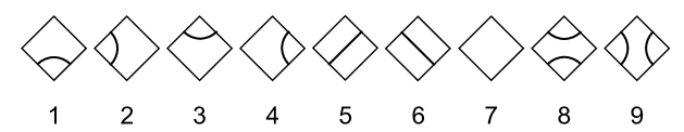
Figure 3: The operators acting on the link patterns.

We denote these basis operators by $\rho^{(1)},\rho^{(2)},..,\rho^{(9)}$ in the order of Fig. 3. By $\rho^{(i)}_{j}$ we denote the operator $\rho^{(i)}$ acting on two adjacent sites $j$ and $j+1$ of a link pattern. It is better to describe graphically the action of these operators Fig. 4.

Figure 4: Here we present few link patterns on which $\rho^{(i)}$ operators act.

The action of $\rho^{(i)}$ on the link patterns should respect the occupation, i.e., the top left and top right occupations of a $\rho^{(i)}_{j}$ should coincide with the occupations of the edges $j$ and $j+1$ (respectively) in the link pattern, otherwise the action gives zero. We notice that $\rho^{(2)},\rho^{(4)},\rho^{(7)}$ and $\rho^{(9)}$ act as projectors on the different occupancies of two edges, $\rho^{(5)}$ and $\rho^{(6)}$ act locally by interchanging an occupied edge with an unoccupied edge, the operator $\rho^{(1)}$ also acts locally by inserting a little arch at the position $j,~{}j+1$ of a link pattern. The two remaining operators $\rho^{(3)}$ and $\rho^{(8)}$, change the global picture, because they connect two existing paths, or close one. In this way, $\rho^{(3)}$ and $\rho^{(8)}$ may produce a loop or a boundary to boundary link as in Fig. 5. We can erase the closed loops at the cost of its weight $n$ and the boundary to boundary link at the cost of its weight $n_{1}$.

Figure 5: The operators $\rho^{(3)}$ and $\rho^{(8)}$ produce a closed loop or a line connecting two vertical boundaries, the line is represented by a dashed semi-circle.

At this point we can turn to the integrability. In order to do this we introduce the $\check{R}$-matrix which is a weighted sum of all nine operators $\rho_{j}^{(i)}$ (see Fig. 6)

$$\check{R}_{j}(z_{j},z_{j+1})=\sum_{i=1}^{9}\rho_{j}^{(i)}r_{i}(z_{j},z_{j+1}).$$ (1)

Figure 6: $\check{R}$-matrix, represented by the shaded lozenge, can be written as a linear combination of the nine plaquettes given in Fig. 3.

The matrix $\check{R}_{j}(z_{j},z_{j+1})$ acts non trivially on the $j$-th and $j+1$-st spaces which carry the rapidities $z_{j}$ and $z_{j+1}$ respectively, on the rest of the lattice spaces it acts as identity. In the graphical notation the rapidities are carried by the oriented straight lines as in Fig. 7.

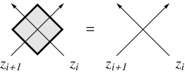
Figure 7: The matrix $\check{R}_{i}(z_{i},z_{i+1})$.

The integrable dilute O$(n)$ loop model is defined by the $\check{R}$-matrix that satisfies the Yang–Baxter (YB) equation [2]. The $\check{R}$-matrix, in fact, depends only on the ratio of the two spectral parameters, hence we may write $\check{R}_{j}(z_{j}/z_{j+1})\propto\check{R}_{j}(z_{j},z_{j+1})$, then the YB equation reads:

$$\check{R}_{i+1}(z/y)\check{R}_{i}(z/x)\check{R}_{i+1}(y/x)=\check{R}_{i}(y/x)\check{R}_{i+1}(z/x)\check{R}_{i}(z/y).$$ (2)

Graphically it is shown in Fig. 8.

Figure 8: The Yang–Baxter equation.

This equation gives the constraints on the weights $r_{i}(z)$. The integrable $R$-matrix was obtained in [23, 22]. In the, so called, additive notation the weights are:

$$r_{1}(x)=r_{3}(x)=\sin 2\lambda\sin x,~{}~{}~{}r_{2}(x)=r_{4}(x)=\sin 2\lambda\sin(3\lambda-x),$$

$$r_{5}(x)=r_{6}(x)=\sin x\sin(3\lambda-x),~{}~{}~{}r_{7}(x)=\sin x\sin(3\lambda-x)+\sin 2\lambda\sin 3\lambda$$

$$r_{8}(x)=\sin x\sin(x-\lambda),~{}~{}~{}r_{9}(x)=\sin(x-2\lambda)\sin(x-3\lambda),$$ (3)

and the loop weight is expressed through the loop fugacity $\lambda$:

$$n=-2\cos 4\lambda.$$ (4)

For our purposes the multiplicative notation is more appropriate (already implied above). In this case we set: $z=e^{ix}$ and $q=e^{i\lambda}$ in (2.1) and by abuse of notation we call the resulting weights $r_{i}(z)$. Up to a common factor of $1/(4z^{2}q^{5})$ we have:

$$r_{1}(z)=r_{3}(z)=-q^{3}\left(q^{4}-1\right)z\left(z^{2}-1\right),~{}~{}~{}r_{2}(z)=r_{4}(z)=-\left(q^{4}-1\right)z\left(q^{6}-z^{2}\right),$$

$$r_{5}(z)=r_{6}(z)=-q^{2}(z^{2}-1)\left(q^{6}-z^{2}\right),~{}~{}~{}r_{7}(z)=q^{8}+q^{2}z^{4}-\left(q^{2}+1\right)\left(q^{8}-q^{4}+1\right)z^{2},$$

$$r_{8}(z)=q^{4}\left(z^{2}-1\right)\left(q^{2}-z^{2}\right),~{}~{}~{}r_{9}(z)=-\left(q^{4}-z^{2}\right)\left(q^{6}-z^{2}\right).$$ (5)

The loop weight becomes $n=-q^{4}-q^{-4}$. Another operator that we will use is the matrix $R_{i}(z)$. It is simply the $\check{R}$ tilted by 45 degrees.

2.2 Open boundary conditions

The boundary of the half infinite strip are represented by the two half infinite vertical lines. One may consider the periodic boundary conditions, i.e. when the two vertical boundaries are identified, closed boundary conditions, i.e. when the loops are reflected from the vertical boundaries. For general non periodic boundary conditions the loops can end at both vertical boundaries. One can also consider open boundary conditions with certain restrictions and various mixed boundary conditions. This is better discussed in [13]. In the case of general open boundary conditions the left and the right boundaries carry the boundary spectral parameters. In the conclusion we will mention how to recover the ground states corresponding to the other non periodic boundary conditions from the ground state corresponding to the general open boundary conditions considered here.

Now we introduce the boundary operators. These operators act on the leftmost and the rightmost points of the link patterns. Graphically they are defined by the plaquettes in Fig. 9.

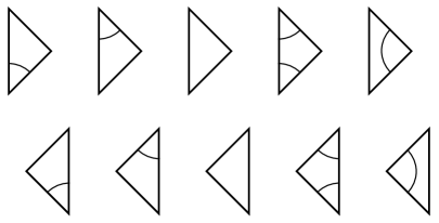
Figure 9: The left and the right boundary operators.

We denote the left boundary operators by $\kappa^{(1)}_{l},..\kappa^{(5)}_{l}$ and the right boundary operators by $\kappa^{(1)}_{r},..,\kappa^{(5)}_{r}$, ordered as in Fig. (9). Few examples of their action on link patterns are presented in Fig. 10.

Figure 10: The action of the $\kappa_{r}$ operators.

We introduce the $K_{l}$-matrix for the left boundary and the $K_{r}$-matrix for the right boundary. The $K$-matrices represent the weighted action of the $\kappa$ operators with the weights: $k_{i}(z_{1},\zeta_{l})$ for the left $K$-matrix and $k_{i}(z_{L},\zeta_{r})$ for the right $K$-matrix. Here, $\zeta_{l}$ and $\zeta_{r}$ are the left and the right boundary rapidities, therefore (Fig. 11)

$$K_{l}(z_{1},\zeta_{l})=\sum_{i=1}^{5}\kappa^{(i)}_{l}k_{i}(z_{1},\zeta_{l}),~{}~{}~{}K_{r}(z_{L},\zeta_{r})=\sum_{i=1}^{5}\kappa^{(i)}_{r}k_{i}(z_{L},\zeta_{r}).$$ (6)

Figure 11: The right $K$-matrix is represented by the shaded triangle.

The action of $K_{i}(z,\zeta)$ switches the rapidity from $z$ to $1/z$. The corresponding graphical notation for $K_{r}(z_{L},\zeta_{r})$ is shown in Fig. 12.

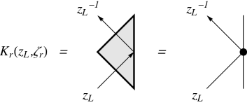
Figure 12: The matrix $K_{r}(z_{L},\zeta_{r})$.

In order to preserve the integrability we need to impose certain conditions on the $k$’s, namely the boundary Yang–Baxter (BYB) equation [26]. For the right boundary it is shown graphically in Fig. 13 and reads:

$$\check{R}_{L-1}(\frac{w}{z})K_{r}(z,\zeta_{r})\check{R}_{L-1}(\frac{1}{wz})K_{r}(w,\zeta_{r})=K_{r}(w,\zeta_{r})\check{R}_{L-1}(\frac{1}{wz})K_{r}(z,\zeta_{r})\check{R}_{L-1}(\frac{w}{z}).$$ (7)

Figure 13: The boundary Yang–Baxter equation.

The integrable boundary weights for the right boundary $K$-matrix in the additive convention are the following [8, 5]:

$$k_{1}(x,\zeta)=k_{2}(x,\zeta)=\zeta\sin 2\lambda\sin 2x,$$

$$k_{3}(x,\zeta)=2\cos\lambda\sin(\frac{3}{2}\lambda+x)-\zeta^{2}n_{1}\sin(\frac{1}{2}\lambda+x)\sin(\frac{1}{2}\lambda-x)\sin(\frac{3}{2}\lambda-x),$$

$$k_{4}(x,\zeta)=-\zeta^{2}\sin 2\lambda\sin 2x\sin(\frac{1}{2}\lambda-x),$$

$$k_{5}(x,\zeta)=\sin(\frac{3}{2}\lambda-x)(2\cos\lambda-\zeta^{2}n_{1}\sin^{2}(\frac{1}{2}\lambda-x)),$$ (8)

here $n_{1}$ is the weight of a loop ending on two boundary points. In order to satisfy BYB we need to assume $n_{1}=n$. There is a different solution to the reflection equation, for more details see [5].

In the multiplicative convention: $z=e^{ix}$ and $q=e^{i\lambda}$ in (2.2), the weights read:

$$k_{1}(z,\zeta)=k_{2}(z,\zeta)=2\zeta q\left(q^{4}-1\right)z\left(z^{4}-1\right),$$

$$k_{3}(z,\zeta)=iq^{1/2}\left(\zeta^{2}n_{1}\left(q-z^{2}\right)\left(qz^{2}-1\right)\left(q^{3}z^{2}-1\right)+4\left(q^{2}+1\right)z^{2}\left(q^{3}-z^{2}\right)\right),$$

$$k_{4}(z,\zeta)=-i\zeta^{2}q^{1/2}\left(q^{4}-1\right)\left(z^{4}-1\right)\left(qz^{2}-1\right),$$

$$k_{5}(z,\zeta)=iq^{1/2}\left(q^{3}z^{2}-1\right)\left(\zeta^{2}n_{1}\left(qz^{2}-1\right)^{2}+4\left(q^{2}+1\right)z^{2}\right),$$ (9)

where we omitted the denominator $8z^{3}q^{3}$ with respect to the definitions (2.2). The transfer matrix $T(t|z_{1},..,z_{L};\zeta_{l},\zeta_{r})$, depicted in Fig. 14, acts in the space of link patterns. It is constructed from the $R$ and $K$ matrices:

$$T(t|z_{1},..,z_{L};\zeta_{l},\zeta_{r})=\text{Tr}\big{(}R_{1}(z_{1}/t)..R_{L}(z_{L}/t)K_{r}(t,\zeta_{r})R_{L}(1/(tz_{L}))..R_{1}(1/(tz_{1}))K_{l}(t^{-1},\zeta_{l})\big{)},$$ (10)

where the trace means that the lower edge of the $K_{l}(t^{-1},\zeta_{l})$ needs to be identified with the left edge of $R_{1}(t,z_{1})$. Due to the YB and the BYB two transfer matrices with different values of $t$ commute:

$$[T(t_{1}),T(t_{2})]=0.$$ (11)

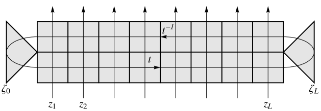
Figure 14: The graphical representation of the transfer matrix.

Other important properties of the transfer matrix coming from the YB and BYB are the commutations with the $\check{R}$:

$$\check{R}_{i}(z_{i},z_{i+1})T(t|z_{1},..,z_{i},z_{i+1},..,z_{L};\zeta_{l},\zeta_{r})=T(t|z_{1},..,z_{i+1},z_{i},..,z_{L};\zeta_{l},\zeta_{r})\check{R}_{i}(z_{i},z_{i+1}),$$ (12)

and with the $K$-matrices

$$K_{l}(z_{1},\zeta_{l})T(t|z_{1},z_{2},..,z_{L};\zeta_{l},\zeta_{r})=T(t|1/z_{1},z_{2},..,z_{L};\zeta_{l},\zeta_{r})K_{l}(z_{1},\zeta_{l}),$$ (13)

$$K_{r}(z_{L},\zeta_{r})T(t|z_{1},..,z_{L-1},z_{L};\zeta_{l},\zeta_{r})=T(t|z_{1},...z_{L-1},1/z_{L};\zeta_{l},\zeta_{r})K_{r}(z_{L},\zeta_{r})$$ (14)

The common ground-state vector of the family of transfer matrices $T(t|z_{1},..,z_{L};\zeta_{l},\zeta_{r})$ parametrized by $t$ we denote by $\Psi_{L}$:

$$T(t|z_{1},..,z_{L};\zeta_{l},\zeta_{r})\Psi_{L}(z_{1},..,z_{L};\zeta_{l},\zeta_{r})\propto\Psi_{L}(z_{1},..,z_{L};\zeta_{l},\zeta_{r}).$$ (15)

The eigenvectors of $T$ can be written in the link pattern basis, in particular:

$$\Psi_{L}(z_{1},..,z_{L};\zeta_{l},\zeta_{r})=\sum_{\pi\in\text{LP}_{L}}\psi_{\pi}(z_{1},..,z_{L};\zeta_{l},\zeta_{r})|\pi\rangle.$$ (16)

Our aim is to understand how to compute the components $\psi_{\pi}$ when the loop weight $n$ (and also $n_{1}$) is equal to $1$.

3 Loop weight $n=1$

In this section we specify our model to the case when $q=e^{i\pi/3}$, then the loop weight $n$ (and we assume also $n_{1}=n$) has the weight equal to$~{}1$. This means that the presence of the closed loops in a configuration does not affect the weight of this configuration. At this point the ground state is a steady state of a stochastic process that can be defined by the Hamiltonian (or transfer matrix) of the dTL model. This happens in analogy with the dense TL loop model at $n=1$ [24]. The ground state entries become the relative probabilities of the occurrence of the corresponding link patterns. Assuming that the transfer matrix is normalized, the ground state eigenvector equation becomes:

$$T(t|z_{1},..,z_{L};\zeta_{l},\zeta_{r})\Psi_{L}(z_{1},..,z_{L};\zeta_{l},\zeta_{r})=\Psi_{L}(z_{1},..,z_{L};\zeta_{l},\zeta_{r}).$$ (17)

This implies the invariance of the probabilities under the addition of two rows of the transfer matrix. Since the transfer matrix is a rational function of the rapidities, we can normalize $\Psi_{L}$ such that its components become coprime polynomials.

We will replace everywhere $q$ by $\omega$ and assume $\omega=e^{i\pi/3}$. The matrices $R$ and $K$ simplify. The $R$-matrix given in (2.1) has a common factor of $\omega/(1-z^{2})$ when $q=\omega$, we omit this factor below and use $r_{i}(z)$ to denote the weights.

$$r_{1}(z)=r_{2}(z)=r_{3}(z)=r_{4}(z)=\omega(\omega+1)z,~{}~{}~{}r_{5}(z)=r_{6}(z)=r_{7}(z)=z^{2}-1,$$

$$r_{8}(z)=-\left(\omega+z\right)\left(\omega^{2}z+1\right),~{}~{}~{}r_{9}(z)=\left(\omega^{2}+z\right)\left(\omega z+1\right).$$ (18)

From now on we will use the parameter $\tilde{\zeta}=-\omega\zeta/2$ instead of $\zeta$ in what follows and in order to simplify the formulae we will omit the tilde. The left $K$-matrix weights read

$$k_{1,l}(z,\zeta_{l})=k_{2,l}(z,\zeta_{l})=-\frac{(\omega+1)\left(z^{2}-1\right)}{z},~{}~{}~{}k_{3,l}(z,\zeta_{l})=\frac{\zeta^{2}\omega+\zeta^{2}\omega z^{4}-\zeta^{2}\omega z^{2}+z^{2}}{\zeta z^{2}},$$

$$k_{4,l}(z,\zeta_{l})=-\frac{\zeta(\omega+1)\left(z^{2}-1\right)\left(\omega-z^{2}\right)}{z^{2}},~{}~{}~{}k_{5,l}(z,\zeta_{l})=-\frac{\left(-\zeta\omega+\zeta z^{2}-z\right)\left(-\zeta\omega+\zeta z^{2}+z\right)}{\zeta z^{2}}.$$ (19)

The weights of the right boundary $K$-matrix are given by $k_{i,r}(z,\zeta)=k_{i,l}(1/z,\zeta)$., they agree with (2.2) up to the denominator $4\zeta z^{2}(z^{2}+1)$.

Acting with the $\check{R}$-matrix on a link pattern gives a sum of the link patterns obtained from the action of the $\rho^{(j)}$ operators, weighted by the corresponding functions $r_{j}$. For example, on a link pattern with two empty sites $n_{i}=0,~{}n_{i+1}=0$, $\check{R}_{i}$ acts by $\rho^{(1)}$ with the probability $r_{1}$ and by $\rho^{(7)}$ with the probability $r_{7}$. Hence, we need to normalize this action with $W=r_{1}+r_{7}$. In fact, the weights (3) are such that for any occupation $n_{i}$ and $n_{i+1}$ the normalization is the same.

$$W(z_{i},z_{i+1})=\left(\omega z_{i}+z_{i+1}\right)\left(\omega^{2}z_{i}+z_{i+1}\right).$$ (20)

Similar arguments apply to the $K$-matrices. The normalizations of $K_{l}$ and $K_{r}$ are:

$$U_{l}(z,\zeta_{l})=-\frac{\left(\omega\zeta_{l}-z^{2}\zeta_{l}+z\right)\left(-\zeta_{l}+\omega z^{2}\zeta_{l}-z\right)}{z^{2}\zeta_{l}},$$ (21)

$$U_{r}(z,\zeta_{r})=\frac{\left(-\omega\zeta_{r}+z^{2}\zeta_{r}+z\right)\left(-\zeta_{r}+\omega z^{2}\zeta_{r}+z\right)}{z^{2}\zeta_{r}}.$$ (22)

Now, using (12) we find

$$\check{R}(z_{i},z_{i+1})\Psi_{L}(z_{1},..,z_{i},z_{i+1},..,z_{L};\zeta_{l},\zeta_{r})=W(z_{i},z_{i+1})\Psi_{L}(z_{1},..,z_{i+1},z_{i},..,z_{L};\zeta_{l},\zeta_{r}),$$ (23)

and also, using (13) and (14):

$$K_{l}(z_{1},\zeta_{l})\Psi_{L}(z_{1},..,z_{L};\zeta_{l},\zeta_{r})=U_{l}(z_{1},\zeta_{l})\Psi_{L}(1/z_{1},..,z_{L};\zeta_{l},\zeta_{r}),$$ (24)

$$K_{r}(z_{L},\zeta_{r})\Psi_{L}(z_{1},..,z_{L};\zeta_{l},\zeta_{r})=U_{r}(z_{L},\zeta_{r})\Psi_{L}(z_{1},..,1/z_{L};\zeta_{l},\zeta_{r}).$$ (25)

Equations (23)- (25) together will be called the $q$KZ equations. This set of equations is a system of functional equations with polynomial solutions. It allows to find all components of the ground state only if a certain set of the components is already known. These components $\psi_{\pi}$ are those which correspond to the link patterns $\pi_{i}=\{0_{1},..,0_{i},-1_{i+1},..,-1_{L}\}$ or $\tilde{\pi}_{i}=\{1_{1},..,1_{L-i-1},0_{L-i},..,0\}$ (here, the index denotes the corresponding site). These are the components which have all empty sites starting from the first (respectively, last) site up to the $i$-th ($L-i$-th) and the rest is connected to the left (right) boundary (Fig. 15). The elements $\psi_{\pi_{0}}$ and $\psi_{\tilde{\pi}_{0}}$ are called the fully nested elements (Fig. 16). They play a special role in our computations since all $\psi_{\pi_{i}}$ as well as $\psi_{\tilde{\pi}_{i}}$ can be obtained from the fully nested elements of larger systems using the recurrence relation to which we turn or discussion now.

Figure 15: Two link patterns $\pi_{2}$ and $\tilde{\pi}_{2}$ at $L=5$.

Figure 16: Two $L=5$ link patterns $\pi_{0}$ and $\tilde{\pi}_{0}$.

We notice that when we set two consecutive rapidities $z_{i}$ and $z_{i+1}$ to $z_{i}\omega$ and $z_{i}/\omega$ the matrix $\check{R}(z_{i},z_{i+1})$ factorizes into two operators

$$\check{R_{i}}(z\omega,z/\omega)=(\omega^{2}+\omega)z^{2}S_{i}M_{i}.$$ (26)

Now using the operator $M_{i}$ we can write

$$M_{i}\check{R_{i}}(z_{i}\omega)R_{i+1}(z_{i}/\omega)=(z_{i}^{2}-1)R_{i}(t,z_{i})M_{i},$$

$$M_{i}\check{R_{i}}(z_{i}/\omega)R_{i+1}(z_{i}\omega)=(z_{i}^{2}-1)R_{i}(t,z_{i})M_{i},$$ (27)

which can be checked by a direct calculation. This equation means that $M$ maps two sites into one site and hence merges the two $R$-matrices into one after the substitution $z_{i}=z_{i}\omega$ and $z_{i+1}=z_{i}/\omega$. The graphical representations of $M$, $S$ and (3) are presented in the figures (17) and (18).

Figure 17: The operators $M_{i}$ and $S_{i}$.

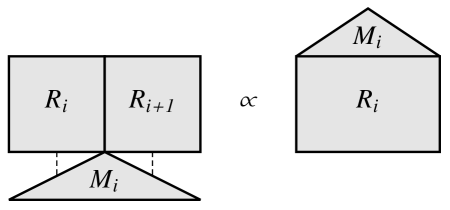
Figure 18: Equation (3).

One can see from (3) (Fig. 18) and the definition of the transfer matrix (10) that by applying $M_{i}$ to the transfer matrix we get:

$$M_{i}T_{L+1}(t|z_{1},..,z_{i}\omega,z_{i}/\omega,z_{i+1},..,z_{L};\zeta_{l},\zeta_{r})\propto T_{L}(t|z_{1},..,z_{i},z_{i+1},..,z_{L};\zeta_{l},\zeta_{r})M_{i},$$ (28)

where we included the indices $L$ and $L+1$ in the transfer matrix to denote the length of the space on which it acts. The proportionality factor is coming from the factors on the right hand sides of (3) and can be eliminated by choosing an appropriate normalization of the transfer matrix. Applying (28) to the ground state we get:

$$M_{i}T_{L+1}(..,z_{i}\omega,z_{i}/\omega,z_{i+1},..)\Psi_{L+1}(..,z_{i}\omega,z_{i}/\omega,z_{i+1},..)\propto$$

$$T_{L}(..,z_{i},z_{i+1},..)M_{i}\Psi_{L+1}(..,z_{i}\omega,z_{i}/\omega,z_{i+1},..),$$ (29)

which becomes

$$M_{i}\Psi_{L+1}(..,z_{i}\omega,z_{i}/\omega,z_{i+1},..)=T_{L}(t|..,z_{i},z_{i+1},..)M_{i}\Psi_{L+1}(..,z_{i}\omega,z_{i}/\omega,z_{i+1},..),$$ (30)

where we omit the dependence on the irrelevant variables for convenience. We obtain the following recurrence relation:

$$M_{i}\Psi_{L+1}(z_{1},..,z_{i}\omega,z_{i}/\omega,z_{i+1},..,z_{L+1};\zeta_{l},\zeta_{r})\propto\Psi_{L}(z_{1},..,z_{i},z_{i+1},..,z_{L};\zeta_{l},\zeta_{r}).$$ (31)

Let us introduce the operator $\mu_{i}$ which projects the ring of polynomials of $L$ variables $\mathbb{C}[z_{1},..,z_{L}]$ onto the ring of polynomials of $L-1$ variables $\mathbb{C}[z_{1},..,\hat{z}_{i+1},..z_{L-1}]$, where $\hat{z}_{i+1}$ means that this variable is absent from the list. Consider a polynomial $f(z_{1},..,z_{L})\in\mathbb{C}[z_{1},..,z_{L}]$, the action of $\mu_{i}$ is defined by

$$\mu_{i}f(z_{1},..,z_{i-1},z_{i},z_{i+1},z_{i+2},..,z_{L})=f(z_{1},..,z_{i-1},z_{i}\omega,z_{i}/\omega,z_{i+2},..,z_{L}).$$ (32)

For example, fix $L=3$ and set $f(z_{1},z_{2},z_{3})=z_{1}^{2}+z_{2}z_{3}+z_{3}^{2}$, then the action of $\mu_{1}$ and $\mu_{2}$ is

$$\mu_{1}\left(z_{1}^{2}+z_{2}z_{3}+z_{3}^{2}\right)=\left(z_{1}\omega\right)^{2}+\left(z_{1}/\omega\right)z_{3}+z_{3}^{2},$$

$$\mu_{2}\left(z_{1}^{2}+z_{2}z_{3}+z_{3}^{2}\right)=z_{1}^{2}+\left(z_{2}\omega\right)\left(z_{2}/\omega\right)+\left(z_{2}/\omega\right)^{2}.$$

The recurrence (31) relates the components of $\Psi_{L+1}$ to the components of $\Psi_{L}$. What we need to do to complete this equation is to find the proportionality factor. In the next section we will see that the knowledge of the fully nested element allows one to find this proportionality factor. Combining the boundary $q$KZ equation with (31) will allow us to find all $\psi_{\pi_{i}}$. Then we will show how to recover the full ground state using the $q$KZ system.

3.1 The $q$KZ equations and the fully nested elements

Let us take a closer look at the $q$KZ equations. First we focus on the bulk $q$KZ. (23) gives $(L-1)$ equation for each link pattern, hence $(L-1)3^{L}$ equations in total. It is sufficient to write a few distinct cases depending on the local connectivity at the sites $i$ and $i+1$ of a link pattern $\pi$ of the component $\psi_{\pi}$. For convenience, we will write $\pi=\{\alpha,n_{i},n_{i+1},\beta\}$, where $\alpha$ and $\beta$ are the parts of $\pi$ on the left and on the right to the sites $n_{i}$ and $n_{i+1}$, respectively. Also, since we will focus only on the sites $i$ and $i+1$ we will not write explicitly the dependence on the variables attached to the other spaces.

1. Both sites $i$ and $i+1$ are occupied.

   a.) The sites $i$ and $i+1$ in $\pi$ are connected via a little arch: $\pi=\{\alpha,1,-1,\beta\}$. In this case (23) gives:

$$W(z_{i},z_{i+1})\psi_{\pi}(..,z_{i+1},z_{i},..)=r_{9}(z_{i},z_{i+1})\psi_{\pi}(..,z_{i},z_{i+1},..)+$$

$$r_{1}(z_{i},z_{i+1})\psi_{\{\alpha,0,0,\beta\}}(..,z_{i},z_{i+1},..)+r_{8}(z_{i},z_{i+1})\sum_{\pi^{\prime}:\rho_{i}^{(8)}\pi^{\prime}=\pi}\psi_{\pi^{\prime}}(..,z_{i},z_{i+1},..).$$ (33)

   b.) The sites $i$ and $i+1$ are not connected to each other:

$$W(z_{i},z_{i+1})\psi_{\pi}(..,z_{i+1},z_{i},..)=r_{9}(z_{i},z_{i+1})\psi_{\pi}(..,z_{i},z_{i+1},..).$$ (34)

2. Both sites $i$ and $i+1$ in $\pi$ are unoccupied

$$W(z_{i},z_{i+1})\psi_{\pi}(..,z_{i+1},z_{i},..)=r_{7}(z_{i},z_{i+1})\psi_{\pi}(..,z_{i},z_{i+1},..)+$$

$$r_{3}(z_{i},z_{i+1})\sum_{\pi^{\prime}:\rho_{i}^{(3)}\pi^{\prime}=\pi}\psi_{\pi^{\prime}}(..,z_{i},z_{i+1},..).$$ (35)

3. Finally, one of the sites $i$ and $i+1$ in $\pi$ is occupied and the other one is unoccupied. There are two distinct cases. Fix $i$, then in both cases we will denote by $\pi^{\prime}$ the link pattern that is obtained from $\pi$ by simply interchanging the occupations $n_{i}$ and $n_{i+1}$ of the sites $i$ and $i+1$ in $\pi$. Both equations have the same form:

$$W(z_{i},z_{i+1})\psi_{\pi}(..,z_{i+1},z_{i},..)=r_{2}(z_{i},z_{i+1})\psi_{\pi}(..,z_{i},z_{i+1},..)+r_{5}(z_{i},z_{i+1})\psi_{\pi^{\prime}}(..,z_{i},z_{i+1},..).$$ (36)

This equation corresponds to the case when $i$ is occupied and $i+1$ is empty, the other equation, i.e. the one for $i$-empty and $i+1$-occupied, is obtained from this one by replacing $r_{2}$ with $r_{4}$ and $r_{5}$ with $r_{6}$, however, in both replacements the corresponding weights are equal.

Now let us turn to the boundary $q$KZ equations. Here, we also have to consider few cases separately. Since the logic is similar for both boundaries we will treat the left boundary only.

1. The first site is occupied.

   a.) The connectivity at the first site is $\pi=\{1,\beta\}$, that means that this site is connected to another site or the boundary on the right:

$$U_{l}(z_{1},\zeta_{l})\psi_{\pi}(1/z_{1},..)=k_{l,5}(z_{1},\zeta_{l})\psi_{\pi}(z_{1},..).$$ (37)

   b.) The connectivity at the first site is $\pi=\{-1,\beta\}$, which means it is connected to the left boundary:

$$U_{l}(z_{1},\zeta_{l})\psi_{\pi}(1/z_{1},..)=k_{l,5}(z_{1},\zeta_{l})\psi_{\pi}(z_{1},..)+k_{l,1}\psi_{\{0,\beta\}}(z_{1},..)+$$

$$k_{l,4}(\psi_{\{1,\beta\}}(z_{1},..)+\psi_{\pi}(z_{1},..)),$$ (38)

2. The site $1$ is unoccupied $\pi=\{0,\beta\}$:

$$U_{l}(z_{1},\zeta_{l})\psi_{\pi}(1/z_{1},..)=k_{l,3}(z_{1},\zeta_{l})\psi_{\pi}(z_{1},..)+k_{l,2}(\psi_{\{1,\beta\}}(z_{1},..)+\psi_{\{-1,\beta\}}(z_{1},..)),$$ (39)

As we already mentioned, finding the fully nested elements is the first important step. Let us take a look at the $q$KZ equations which involve the fully nested elements, i.e. (34), first for $\pi_{0}$. Let us fix $i=1$, then this equation after canceling the common factors gives:

$$(\omega z_{1}+z_{2})\psi_{\pi_{0}}(z_{2},z_{1},..)=(\omega z_{2}+z_{1})\psi_{\pi_{0}}(z_{1},z_{2},..).$$ (40)

This means $\psi_{\pi_{0}}$ has the factor $(\omega z_{1}+z_{2})$ and is symmetric in $z_{1},z_{2}$ in the remaining part, which we denote by $\psi^{(1)}_{\pi_{0}}$:

$$\psi_{\pi_{0}}(z_{1},z_{2},..)=(\omega z_{1}+z_{2})\psi^{(1)}_{\pi_{0}}(z_{1},z_{2},..).$$ (41)

Now if we fix $i=2$ in (34) we see that $\psi^{(1)}_{\pi_{0}}$ must contain the factor $(\omega z_{2}+z_{3})$ and taking into account its symmetries it also must contain the factor $(\omega z_{1}+z_{3})$, we get

$$\psi_{\pi_{0}}(z_{1},z_{2},..)=(\omega z_{1}+z_{2})(\omega z_{2}+z_{3})(\omega z_{1}+z_{3})\psi^{(2)}_{\pi_{0}}(z_{1},z_{2},z_{3},..).$$ (42)

We can proceed in the same manner for $i=3,..,L$ and what we obtain in the end is:

$$\psi_{\pi_{0}}(z_{1},z_{2},..)=\psi^{(L-1)}_{\pi_{0}}(z_{1},..,z_{L})\prod_{1\leq i<j\leq L}(\omega z_{i}+z_{j}).$$ (43)

Here, $\psi^{(L-1)}_{\pi_{0}}$ is symmetric in all variables.

The right boundary $q$KZ equation that involves the $\psi_{\pi_{0}}$ (the right boundary analog of (37)) gives:

$$\frac{\left(-\zeta_{r}+\zeta_{r}\omega z_{L}^{2}-z_{L}\right)}{\zeta_{r}z_{L}}\psi_{\pi_{0}}\left(..,1/z_{L}\right)=-\frac{\left(-\zeta_{r}\omega+\zeta_{r}z_{L}^{2}+z_{L}\right)}{\zeta_{r}z_{L}}\psi_{\pi_{0}}(..,z_{L}),$$ (44)

which holds when:

$$\psi_{\pi_{0}}(..,z_{L})=\frac{\left(-\zeta_{r}+\omega\zeta_{r}z_{L}^{2}-z_{L}\right)}{\zeta_{r}z_{L}}\bar{\psi}_{\pi_{0}}(..,z_{L}),$$ (45)

and $\bar{\psi}_{\pi_{0}}(..,z_{L})=\bar{\psi}_{\pi_{0}}(..,1/z_{L})$. At this point it is convenient to reparametrize $\zeta_{r}$ and $\zeta_{l}$ as follows:

$$\zeta_{r}=\omega\frac{x_{r}}{x_{r}^{2}+1},~{}~{}~{}\zeta_{l}=\omega\frac{x_{l}}{x_{l}^{2}+1}.$$ (46)

Then, equation (45) reads:

$$\psi_{\pi_{0}}(..,z_{L})=\frac{\omega(\omega x_{r}+z_{L})(\omega+x_{r}z_{L})}{x_{r}z_{L}}\bar{\psi}_{\pi_{0}}(..,z_{L}).$$ (47)

Combining this with (43) we obtain:

$$\psi_{\pi_{0}}(z_{1},z_{2},..,z_{L};\zeta(z_{L+1}))=\psi_{\pi_{0}}^{*}(z_{1},..,z_{L},z_{L+1})\prod_{1\leq i<j\leq L+1}\frac{(\omega z_{i}+z_{j})(1+\omega z_{i}z_{j})}{z_{i}z_{j}},$$ (48)

where we replaced $x_{r}$ by $z_{L+1}$. The prefactor in this expression $\psi_{\pi_{0}}^{*}$ is symmetric in all $z_{i}$’s as well as in $z_{i}\rightarrow z_{i}^{-1}$. That is all what we can deduce from the $q$KZ system about the fully nested element $\psi_{\pi_{0}}$. In the same manner we find that:

$$\psi_{\tilde{\pi}_{0}}(z_{1},z_{2},..,z_{L};\zeta(z_{0}))=\psi_{\tilde{\pi}_{0}}^{*}(z_{0},z_{1},..,z_{L})\prod_{0\leq i<j\leq L}\frac{(\omega z_{i}+z_{j})(\omega+z_{i}z_{j})}{z_{i}z_{j}}.$$ (49)

Here $z_{0}$ replaces $x_{l}$ and the prefactor $\psi_{\tilde{\pi}_{0}}^{*}$ is symmetric in $\{z_{0}^{\pm 1},z_{1}^{\pm 1},..,z_{L}^{\pm 1}\}$. Both $\psi_{\pi_{0}}^{*}$ and $\psi_{\tilde{\pi}_{0}}^{*}$ are transparent to the $q$KZ equations, hence we assume that they do not depend on $z_{i}$’s.

3.2 The recurrence relation

In this section we complete (31) by deriving the proportionality factor. In order to do that let us figure out first what does the mapping (31) mean for the components of the ground state. This mapping consists of two parts: the action of $\mu_{i}$ and the action of $M_{i}$. Since the operator $M_{i}$ maps the link patterns of size $L+1$ to the link patterns of size $L$ it induces the correspondence between the components of $\Psi_{L+1}$ and $\Psi_{L}$. $M_{i}$ acts on the sites $i$ and $i+1$ by mapping the link patterns of LP_L+1 with $n_{i}=1,~{}n_{i+1}=-1$ or $n_{i}=0,~{}n_{i+1}=0$ to the link patterns of LP_L with $n_{i}=0$, more explicitly $\{\alpha,1,-1,\beta\}\in\text{LP}_{L+1}$ maps to $\{\alpha,0,\beta\}\in\text{LP}_{L}$ and $\{\alpha,0,0,\beta\}\in\text{LP}_{L+1}$ maps to $\{\alpha,0,\beta\}\in\text{LP}_{L}$. The link patterns in LP_L+1 which have $n_{i}=\pm 1,~{}n_{i+1}=0$ or $n_{i}=0,~{}n_{i+1}=\pm 1$ are mapped to the link patterns of LP_L with $n_{i}=\pm 1$, for example $\{\alpha,1,0,\beta\}\in\text{LP}_{L+1}$ maps to $\{\alpha,1,\beta\}\in\text{LP}_{L}$ (Fig. 19).

Figure 19: The action of the operator $M_{2}$.

Note, however, that all components with $n_{i}=-1,~{}n_{i+1}=\pm 1$ and $n_{i}=1,~{}n_{i+1}=1$, due to the $q$KZ equation (34) acquire the factor of $z_{i}\omega+z_{i+1}$. This factor vanishes under the action of $\mu_{i}$ since $\omega=e^{i\pi/3}$. Therefore for some link patters $\alpha$ and $\beta$ the recurrence (31) implies

$$\mu_{i}\psi_{\alpha,n_{i}=-1,n_{i+1}=\pm 1,\beta}(..,z_{i},z_{i+1},..)=\mu_{i}\psi_{\alpha,n_{i}=1,n_{i+1}=1,\beta}(..,z_{i},z_{i+1},..)=0,$$ (50)

$$\mu_{i}\psi_{\alpha,n_{i}=1,n_{i+1}=-1,\beta}(..,z_{i},z_{i+1},..)=F_{i}(z_{1},..,\hat{z}_{i+1},..,z_{L})\psi_{\alpha,n_{i}=0,\beta}(..,z_{i},..),$$ (51)

$$\mu_{i}\psi_{\alpha,n_{i}=1,n_{i+1}=0,\beta}(..,z_{i},z_{i+1},..)=F_{i}(z_{1},..,\hat{z}_{i+1},..,z_{L})\psi_{\alpha,n_{i}=1,\beta}(..,z_{i},..),$$ (52)

$$\mu_{i}\psi_{\alpha,n_{i}=0,n_{i+1}=1,\beta}(..,z_{i},z_{i+1},..)=F_{i}(z_{1},..,\hat{z}_{i+1},..,z_{L})\psi_{\alpha,n_{i}=1,\beta}(..,z_{i},..),$$ (53)

$$\mu_{i}\psi_{\alpha,n_{i}=0,n_{i+1}=0,\beta}(..,z_{i},z_{i+1},..)=F_{i}(z_{1},..,\hat{z}_{i+1},..,z_{L})\psi_{\alpha,n_{i}=0,\beta}(..,z_{i},..).$$ (54)

The factor $F_{i}(z_{1},..,z_{L})$ is exactly the proportionality factor in (31), and the label $i$ denotes the site on which $\mu_{i}$ is applied. $F_{i}$ also depends on $\zeta_{l}$ and $\zeta_{r}$ which we did not indicate explicitly.

Now we would like to obtain the explicit form of the function $F_{i}$. In order to do that we need to consider the left boundary $q$KZ equation for the element $\psi_{\pi_{0}}$ which is given by (3.1) and apply twice the $\mu_{1}$ operator to this equation. We find

$$\mu_{1}U_{l}(z_{1},\zeta_{l})\psi_{\pi_{0}}(1/z_{1},..)=\mu_{1}k_{l,5}(z_{1},\zeta_{l})\psi_{\pi_{0}}(z_{1},..)+$$

$$\mu_{1}k_{l,1}(z_{1},\zeta_{l})\psi_{\pi_{1}}(z_{1},..)+\mu_{1}k_{l,4}(z_{1},\zeta_{l})(\psi_{\{1,-1..,-1\}}(z_{1},..)+\psi_{\pi_{0}}(z_{1},..)).$$ (55)

Using (50), (53) and (51) we obtain:

$$U_{l}(z_{1}\omega,\zeta_{l})\psi_{\pi_{0}}(1/(z_{1}\omega),z_{1}/\omega,z_{2},..)=$$

$$F_{1}(z_{1},..,\hat{z}_{i+1},..)(k_{l,1}(z_{1}\omega,\zeta_{l})\psi_{\pi_{0}}(z_{1},..)+k_{l,4}(z_{1}\omega,\zeta_{l})\psi_{\pi_{1}}(z_{1},..)).$$ (56)

Applying $\mu_{1}$ again we arrive at an equation containing the $F$’s and the fully nested elements. It can be rewritten in the form

$$U_{l}(z_{1}\omega^{2},\zeta_{l})\psi_{\pi_{0}}(1/(z_{1}\omega^{2}),z_{1},z_{1}/\omega,z_{2},..,z_{L})=$$

$$F_{1}(z_{1}\omega,z_{1}/\omega,..,z_{L})F_{1}(z_{1},..,z_{L})k_{l,4}(z_{1}\omega^{2},\zeta_{l})\psi_{\pi_{0}}(z_{1},..,z_{L}),$$ (57)

where $\psi_{\pi_{0}}$ appearing on the left hand side depends on $L+2$ arguments and is the $\pi_{0}$ component of the ground state on the strip with $L+2$ sites while $\psi_{\pi_{0}}$ on the right and side depends on $L$ arguments and is the $\pi_{0}$ component of the ground state on the strip with $L$ sites. Plugging here the explicit form of $\psi_{\pi_{0}}$ we find that the choice

$$F_{i}(z_{1},..,z_{L};\zeta_{l}(z_{0}),\zeta_{r}(z_{L+1}))=\prod_{0\leq j\neq i\leq L+1}\frac{(z_{i}+z_{j})(z_{i}z_{j}+1)}{z_{i}z_{j}},$$ (58)

satisfies (3.2) with $i=1$, provided we choose appropriately the constant $\psi_{\pi_{0}}^{*}$. Although we computed (58) for $i=1$, it is also true for $i>1$. One can easily see this by combining this recurrence relation with the $q$KZ equation.

3.3 Computation of the $\psi_{\pi_{i}}$ components

So far we found only the fully nested elements $\psi_{\pi_{0}}$ and $\psi_{\tilde{\pi}_{0}}$. The only $q$KZ equation that relates the fully nested element with others is (3.1), however, it has two unknowns: $\psi_{\{1,-1..,-1\}}$ and $\psi_{\pi_{1}}=\psi_{\{0,-1,..,-1\}}$. As we already saw, after the action of $\mu_{1}$ one of the two unknowns in (3.1) disappear and we arrive at (3.2), hence we can express the element $\psi_{\pi_{1}}$ in terms of $\psi_{\pi_{0}}$ and (3.1) gives us the second unknown $\psi_{\{1,-1..,-1\}}$.

In general, (3.2) holds if we replace $\pi_{0}$ by $\pi=\{-1,-1,\alpha\}$ for any $\alpha$. Using (3.2) we can map the component $\psi_{\{-1,-1,\alpha\}}$ and $\psi_{\{-1,\alpha\}}$ of the ground state $\Psi_{L+1}$ and $\Psi_{L}$ (respectively) to the components $\psi_{\{0,\alpha\}}$ of the ground state $\Psi_{L}$:

$$\psi_{\{0,\alpha\}}(z_{1},z_{2},..,z_{L}))= k_{l,4}^{-1}(z_{1}\omega,\zeta_{l})\bigg{(}U_{l}(z_{1}\omega,\zeta_{l})\frac{\psi_{\{-1,-1,\alpha\}}(1/(z_{1}\omega),z_{1}/\omega,z_{2},..,z_{L})}{F_{1}(z_{1},..,z_{L})}+$$

$$k_{l,1}(z_{1}\omega,\zeta_{l})\psi_{\{-1,\alpha\}}(z_{1},z_{2},..,z_{L})\bigg{)}.$$ (59)

This equation is the first important ingredient in the computation of $\psi_{\pi_{i}}$. The second ingredient is (36) which allows one to compute the component $\psi_{\{\alpha,0,\pm 1,\beta\}}$ if the component $\psi_{\{\alpha,\pm 1,0,\beta\}}$ is known and vice versa. The latter means all components with a fixed relative connectivity of the lines (relative positions of $+1$’s and $-1$’s in $\pi$) form an equivalence class w.r.t. the action of the operators (see Fig. 20)

$$\eta_{i}=\frac{W(z_{i},z_{i+1})}{r_{5}(z_{i},z_{i+1})}(\tau_{i}-1)+1,$$ (60)

$$\text{where}~{}~{}~{}\tau_{i}f_{(}..,z_{i},z_{i+1},..)=f(..,z_{i+1},z_{i},..),$$

thus, we get the identities:

$$\psi_{\{\alpha,\pm 1_{i},0_{i+1},\beta\}}=\eta_{i}\psi_{\{\alpha,0_{i},\pm 1_{i+1},\beta\}},$$ (61)

$$\psi_{\{\alpha,0_{i},\pm 1_{i+1},\beta\}}=\eta_{i}\psi_{\{\alpha,\pm 1_{i},0_{i+1},\beta\}}.$$ (62)

Plugging $\eta_{1}\psi_{\pi_{1}}(z_{1},..,z_{L})$ and $\eta_{2}\eta_{1}\psi_{\pi_{1}}(z_{1},..,z_{L+1})$ into (3.3) gives $\psi_{\pi_{2}}$. It is clear now that by substituting:

$$\psi_{\{-1,\alpha\}}(z_{1},..,z_{L})=\prod_{k=0}^{i-1}\eta_{i-k}\psi_{\pi_{i}}(z_{1},..,z_{L}),$$ (63)

$$\psi_{\{-1,-1,\alpha\}}(z_{1},..,z_{L+1})=\prod_{k=0}^{i-1}\eta_{i-k+1}\eta_{i-k}\psi_{\pi_{i}}(z_{1},..,z_{L+1}),$$ (64)

into (3.3) we can inductively obtain all $\psi_{\pi_{i}}$. Note, that the (3.1) for $\pi=\{-1,-1,\alpha\}$ where $\alpha$ contains $0$’s and/or $-1$’s allows one to obtain all elements $\psi_{\pi}$ with $\pi=\{1,-1,\alpha\}$. Using $\eta_{i}$’s we also get all elements in the equivalence of $\psi_{\{1,-1,\alpha\}}$. Now we can turn to the computation of the other elements of the ground state $\Psi_{L}$.

Figure 20: Equivalence class of the element $\pi=\{0,1,-1\}$.

Figure 21: Elements corresponding to nonequivalent link patterns of $\Psi_{4}$ can be computed using only s (3.2), (3.1), (63) and (64).

3.4 Dyck paths and the ground state components

As in [11], a good way to see how the components of $\Psi_{L}$ can be computed is to turn to the Dyck path formulation. The set of link patterns of length $L$ is the set $\mathbb{Z}_{3}^{\otimes L}$. To any $\pi$ we associate a unique Dyck path in the following way. Reading $\pi$ from left to right, every $1$ corresponds to the north east (NE) step, every $-1$ corresponds to the south east (SE) step and every $0$ corresponds to the horizontal east (E) step. For example, the link pattern $\{-1,-1,0,1,1,0,0,-1,-1,1\}$ is represented by the sequence of moves {SE,SE,E,NE,NE,E,E,SE,SE,NE} which is a Dyck path given in Fig. 22.

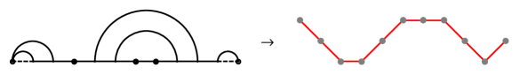
Figure 22: The link pattern $\{-1,-1,0,1,1,0,0,-1,-1,1\}$ and the corresponding Dyck path. The ending and the beginning of each step in the Dyck path is marked by a small disk on the picture.

A few distinguished Dyck paths are those which correspond to the fully nested link patterns (see Fig. 23).

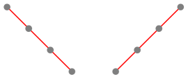
Figure 23: The Dyck paths of $\pi=\{-1,-1,-1\}$ and $\tilde{\pi}=\{1,1,1\}$.

The area under the Dyck paths can be split (in a non unique way) into a few boundary triangles $t_{l,1}$, $t_{l,2}$, $t_{r,1}$ and $t_{r,2}$, bulk triangles $t^{(1)}$ and $t^{(2)}$ and lozenges $l^{(1)}$ and $l^{(2)}$ depicted in Fig. 24. Note, that we need to supplement the bulk triangles and lozenges with an index $j$, then by $t^{(i)}_{j}$ and $l^{(i)}_{j}$ we will denote the operator $t^{(i)}$, respectively $l^{(i)}$, acting at the position $j$.

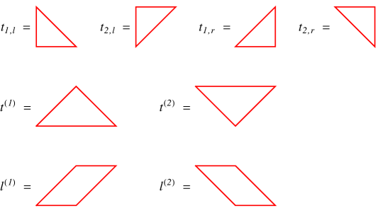
Figure 24: The left boundary $t_{1,l}$, $t_{2,l}$, right boundary $t_{1,r}$, $t_{2,r}$, the bulk $t^{(1)}$, $t^{(2)}$ triangles and the bulk rhombi $l^{(1)}$, $l^{(2)}$.

Each Dyck path can be build by concatenation of these primitives starting from a reference Dyck path. For example, if the reference Dyck path is $\pi_{e}=\{0,0,..,0\}$ the Dyck path $\pi=\{-1,-1,0,1,1,0,0,-1,-1,1\}$, depicted on the Fig. (25), is constructed, e.g. as follows

$$\pi=t_{6}^{(2)}t_{7}^{(1)}t_{5}^{(1)}t_{1,l}t_{7}^{(2)}t_{5}^{(2)}t_{2,l}t_{1}^{(1)}t_{4}^{(1)}t_{6}^{(1)}t_{8}^{(1)}t_{1,r}\pi_{e}.$$ (65)

Similarly, as one link pattern can be converted into another upon the action of a product of $\rho_{i}$ operators, one Dyck path can be converted into another one by attaching or removing rhombi $l^{(i)}$ and triangles $t^{(i)}$ and $t_{i,l/r}$.

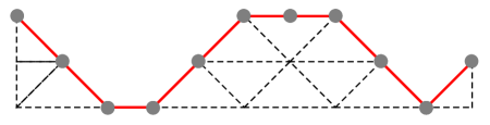
Figure 25: Onepossible decomposition of the Dyck path $\{-1,-1,0,1,1,0,0,-1,-1,1\}$.

Now we introduce the notion of partial ordering on the Dyck Paths. A path $\pi_{1}$ is contained in another path $\pi_{2}$: $\pi_{1}\prec\pi_{2}$ if $\pi_{1}$ can be completed to $\pi_{2}$ by adding to it triangles and lozenges. To make this notion less ambiguous we need to indicate, for example, what is the largest Dyck path w.r.t. all other Dyck paths. Let us choose the element $\pi_{0}$ to be the largest, then the smallest element will be $\tilde{\pi}_{0}$. This means that the addition of the triangles or lozenges to the element $\pi_{0}$ or the removal of the triangles or lozenges from the element $\tilde{\pi}_{0}$ is forbidden. Hence all Dyck paths are contained in the region surrounded by the triangle $D_{L}=\{\{0,L\},\{L,0\},\{0,-L\}\}$. This region $D_{L}$ is depicted in Fig. 26.

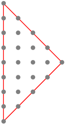
Figure 26: The domain $D_{L}$. The gray disks represent the nodes which the possible Dyck paths may visit.

In order to compute the remaining elements of the ground state we will need the (3.1), which we rewrite in the following form for $\pi=\{\alpha,0,0,\beta\}$:

$$\delta_{i}\psi_{\{\alpha,0,0,\beta\}}(..,z_{i},z_{i+1},..)-\psi_{\{\alpha,1,-1,\beta\}}(..,z_{i},z_{i+1},..)=\sum_{\begin{subarray}{c}\pi^{\prime}:\rho_{i}^{(8)}\pi^{\prime}=\pi\\ \pi^{\prime}\neq\pi\end{subarray}}\psi_{\pi^{\prime}}(..,z_{i},z_{i+1},..),$$ (66)

where we defined the operator $\delta_{i}$:

$$\delta_{i}=\frac{W(z_{i},z_{i+1})\tau_{i}-r_{7}(z_{i},z_{i+1})}{r_{1}(z_{i},z_{i+1})}.$$ (67)

The boundary $q$KZ with $\pi=\{0,\alpha\}$ (39) is also useful to rewrite as:

$$\gamma_{l}\psi_{\{0,\alpha\}}(z_{1},..)-\psi_{\{1,\alpha\}}(z_{1},..)=\psi_{\{-1,\alpha\}}(z_{1},..),$$ (68)

where we defined the operator $\gamma_{l}$:

$$\gamma_{l}=\frac{U_{l}(z_{1},\zeta_{l})\sigma_{l}-k_{l,3}(z_{1},\zeta_{l})}{k_{l,2}(z_{1},\zeta_{l})},~{}~{}~{}~{}\text{and}~{}~{}\sigma_{l}f(z_{1},z_{2},..)=f(1/z_{1},z_{2},..).$$ (69)

Note, in both equations (66) and (68) in the right hand sides we can identify the smallest elements in those equations in the sense of the ordering of Dyck paths. The idea below is to compute one by one elements $\psi_{\pi}$ in the direction of decreasing $\pi$, therefore (66) and (68) will always have one unknown which will be the element corresponding to the minimal $\pi$ within a given equation.

We proceed as follows. Let us consider the elements corresponding to the Dyck paths passing through the points $\{j,L-j\}$ for $0\leq j\leq L$, i.e. the points on the right boundary of the domain $D_{L}$. Take $j=0$, there is only one path which passes through this point and it corresponds to $\psi_{\pi_{0}}$. Next we take $j=1$, there are two paths corresponding to $\psi_{1}$ and $\psi_{2}$ in Fig. 27. Next we take $j=2$, these paths are labeled by $\psi_{i}$ with $i=3,..,8$ on the Fig. (27). We already know the following components: $\psi_{0}$, $\psi_{1}$, $\psi_{2}$, $\psi_{3}$ and $\psi_{4}$. Here, $\psi_{0}$ is the fully nested component (48), while the others follow from (3.3), (61), (62) and (68).

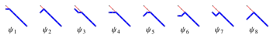
Figure 27: The Dyck paths (thick blue line) passing through the point $\{1,L-1\}$ ($\psi_{1}$ and $\psi_{2}$) and the Dyck paths passing through the point $\{2,L-2\}$ ($\psi_{j},~{}~{}j=3,..,8$) of the domain $D_{L}$. For the reference we also included the north to east edge of the $D_{L}$ triangle.

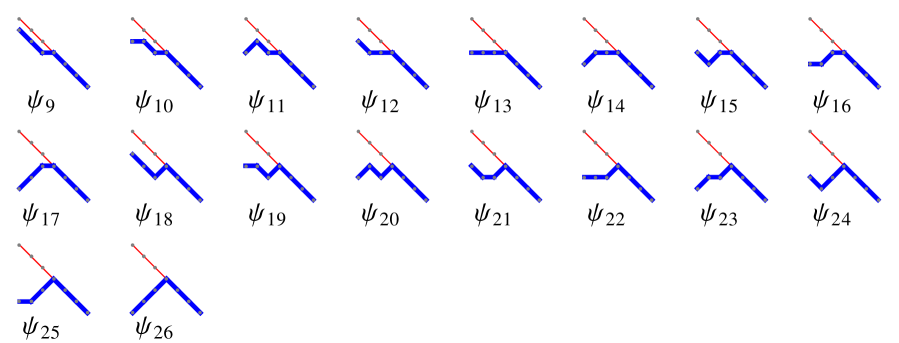
Figure 28: Dyck paths passing the $\{3,L-3\}$ point of the domain $D_{L}$.

Every unknown $\psi_{i}$ on this figure we can obtain from a few $\psi_{j}$’s with $j<i$ and $\psi_{0}=\psi_{\pi_{0}}$. Indeed, we have:

$$\psi_{5}=\gamma_{l}\psi_{4}-\psi_{3},~{}~{}~{}\psi_{6}=\eta_{1}\psi_{5},~{}~{}\psi_{7}=\delta_{1}\psi_{4}-\psi_{2}-\psi_{0},~{}~{}~{}\psi_{8}=\gamma_{l}\psi_{6}-\psi_{7}.$$ (70)

Let us take now $j=3$, the Dyck paths passing through this point are depicted on the Fig. 28. Among these we already know the components which are in the equivalence class w.r.t. the action of $\eta$ of $\psi_{\pi_{i}}$ and $\psi_{i}$ from Fig. 27. These components are: $\psi_{9}$, $\psi_{10}$, $\psi_{11}$, $\psi_{12}$, $\psi_{13}$, the rest are:

$$\psi_{14}=\gamma_{l}\psi_{13}-\psi_{12},~{}~{}~{}\psi_{15}=\delta_{1}\psi_{13}-\psi_{11}-\psi_{9},~{}~{}~{}\psi_{16}=\eta_{1}\psi_{14},~{}~{}~{}\psi_{17}=\gamma_{l}\psi_{16}-\psi_{15},~{}~{}~{}$$

$$\psi_{18}=\delta_{2}\psi_{12}-\psi_{7}-\psi_{0},~{}~{}~{}\psi_{19}=\eta_{1}\eta_{2}\psi_{15},~{}~{}~{}\psi_{20}=\gamma_{l}\psi_{19}-\psi_{18},~{}~{}~{}\psi_{21}=\eta_{1}\psi_{15},~{}~{}~{}$$

$$\psi_{22}=\eta_{2}\eta_{1}\psi_{14},~{}~{}~{}\psi_{23}=\gamma_{l}\psi_{22}-\psi_{21},~{}~{}~{}\psi_{24}=\delta_{1}\psi_{22}-\psi_{18}-\psi_{20}-\psi_{8},~{}~{}~{}$$

$$\psi_{25}=\eta_{1}\eta_{2}\psi_{17},~{}~{}\psi_{26}=\gamma_{l}\psi_{25}-\psi_{24}.$$ (71)

These computations are valid for any $L$ larger or equal to $3$. In the latter case it gives all 27 components. In this calculation we have selected the reference state to be $\psi_{\pi_{0}}$. Then we found that any component $\psi_{\pi}$ can be expressed through a number of components associated to larger Dyck paths than the path $\pi$. All computations can be done in a similar manner using $\psi_{\tilde{\pi}_{0}}$ as the reference. The explicit results for $L=1,2$ are presented in Appendix A.

4 Discussions

Usually, integrable models at finite size are studied via the Bethe ansatz, in which case the eigenstates of the transfer matrix depend on the Bethe roots. One then has to solve the set of nonlinear Bes in order to obtain the eigenstates and the eigenvalues. In our case, following the prescription developed for the TL model at $n=1$ [12], we were able to find the ground state eigenvector explicitly for finite systems avoiding the complicated nonlinear equations. Indeed, if we take our ground state $\Psi_{L}$ in the spin basis (which amounts to a linear transformation on $\Psi_{L}$, see e.g. [23]) this will correspond to a certain state of the 19 vertex Izergin–Korepin (IK) model at $q=e^{i\pi/3}$. The algebraic Bethe ansatz for this model with periodic boundary conditions was found by Tarasov [27]. In the case of periodic boundary conditions and small system sizes we verified that the Bethe ansatz eigenstate agrees with the calculation based on the $q$KZ equation of the type presented in this paper.

The approach that we are using allows us to find (strictly speaking to conjecture) closed expressions for a few components of the ground state vector. These components are the fully nested element $\psi_{\pi_{0}}$ and a few others which are “close” enough to $\psi_{\pi_{0}}$ and expressed through $\psi_{\pi_{0}}$ itself. For example $\psi_{\pi_{1}}$ follows from (3.3). As we go further away from these components the complexity of the computations increases rapidly, that is why we are limited to only a few components. Another component which we can write in a closed form for arbitrary $L$ is $\psi_{e}$. It turns out that this component is proportional to $Z_{L}$-the sum of all components of $\Psi_{L}$. $Z_{L}$ is the normalization of the ground state $\Psi_{L}$, thus it is an important quantity for the computation of correlation functions. One such correlation function is the boundary to boundary current. It was computed for the TL model in [6] and in the dilute TL case it is the subject of the paper [9]. Due to the relation of the dilute TL model at $n=1$ to the critical site percolation, $Z_{L}^{2}$ plays the role of the partition function in the critical percolation on an infinite strip. We compute $Z_{L}$ in [15].

We would like to stress here that we were dealing with the generic open boundary conditions. In this case the boundaries carry the parameters $\zeta_{l}$ and $\zeta_{r}$. From our state $\Psi_{L}$ we can recover the ground state $\Psi_{L}^{c}$ of the loop model with closed (also called reflecting) boundary conditions simply by sending the parameters $\zeta$ to $0$ (where $\Psi_{L}$ is assumed to be properly normalized). In this case one could study an interesting correlation function: the current going from $-\infty$ to $+\infty$ along the strip. This current was studied in the paper [16] for the TL $n=1$ loop model. One could also send $\zeta$ to infinity (with a proper normalization), then the corresponding $K$-matrix is a combination of $\kappa_{3}$, $\kappa_{4}$ and $\kappa_{5}$. This can be an interesting case to study, since as it is stressed in [5] there are a few solutions $K^{(1)}$ and $K^{(2)}$ to the reflection equation. The solution $K^{(1)}$ is the one we used here. The solution $K^{(2)}$ is a combination of only three operators $\kappa_{3}$, $\kappa_{4}$ and $\kappa_{5}$. The two solutions are independent for generic $n$, but for $n=1$ $K^{(2)}$ is the $\zeta\rightarrow\infty$ limit of $K^{(1)}$. Hence to compute the ground state with $K^{(2)}$-matrix one needs to send $\zeta$ to infinity in our solution.

The next point we would like to stress is the computation of the ground state at $n=0$. It turns out that at $n=0$ the dilute TL loop model also possesses a polynomial ground state and the $q$KZ together with the recurrence relations remain intact. The algorithm of the computation of $\Psi_{L}$ presented here remains applicable.

Appendix A Appendix

In this appendix we present explicit expressions for the polynomial ground state $\Psi_{L}$ for $L=1,~{}2$. The $\Psi_{1}$ components are:

$$\psi_{-1}=\frac{\omega\left(x_{r}+\omega z_{1}\right)\left(\omega z_{1}x_{r}+1\right)}{z_{1}x_{r}},$$ (72)

$$\psi_{1}=\frac{\omega\left(\omega x_{l}+z_{1}\right)\left(z_{1}x_{l}+\omega\right)}{z_{1}x_{l}},$$ (73)

$$\psi_{0}=\frac{\omega^{2}\left(z_{1}x_{l}^{2}x_{r}+z_{1}^{2}x_{l}x_{r}+z_{1}x_{l}x_{r}^{2}+x_{l}x_{r}+z_{1}x_{l}+z_{1}x_{r}\right)}{z_{1}x_{l}x_{r}}.$$ (74)

The last component can be written in terms of the elementary symmetric polynomials

$$E_{m}(z_{1},..,z_{L}) =\sum_{1\leq i_{1}<,..,<i_{m}}z_{i_{1}}..z_{i_{m}},$$

$$E_{m}(z_{1},..,z_{L}) =0~{}~{}~{}\text{for}~{}~{}~{}m<0,~{}~{}~{}\text{and}~{}~{}~{}m>L,$$

as follows:

$$\psi_{0}(z_{1};x_{l},x_{r})=\frac{\omega^{2}(E_{2}+E_{1}E_{3})}{E_{3}},$$ (75)

in which $E_{i}=E_{i}(x_{l},z_{1},x_{r})$. The choice of the constant prefactor of the nested elements in (72) and (73) fixes the constants $\psi_{\pi_{0}}^{*}$ and $\psi_{\tilde{\pi}_{0}}^{*}$ from (48) and (49). Hence we will not write the nested elements for $L=2$. The remaining components of $\Psi_{2}$ up to the actions of $\eta_{i}$ are:

$$\psi_{1,-1}=\frac{\left(\omega x_{l}+z_{1}\right)\left(z_{1}x_{l}+\omega\right)\left(x_{r}+\omega z_{2}\right)\left(\omega z_{2}x_{r}+1\right)}{z_{1}^{2}z_{2}^{2}x_{l}^{2}x_{r}^{2}}(E_{3}+E_{1}E_{4}),$$

$$\psi_{0,-1}=\frac{\omega\left(x_{r}+\omega z_{2}\right)\left(\omega z_{2}x_{r}+1\right)}{z_{1}^{2}z_{2}^{2}x_{l}x_{r}^{2}}\bigg{(}z_{1}(1+z_{2}^{2})(E_{2}(x_{l},z_{1},x_{r})+E_{1}(x_{l},z_{1},x_{r})E_{3}(x_{l},z_{1},x_{r}))+$$

$$z_{2}\big{(}\left(z_{1}^{2}+1\right)x_{l}\left(x_{r}+z_{1}\right)\left(z_{1}x_{r}+1\right)+z_{1}(x_{1}^{2}+1)\left((\omega+1)x_{r}\left(\omega^{2}+z_{1}^{2}\right)+z_{1}(x_{r}^{2}+1)\right)\big{)}\bigg{)},$$

$$\psi_{1,0}=\frac{\omega\left(\omega x_{l}+z_{1}\right)\left(z_{1}x_{l}+\omega\right)}{z_{1}^{2}z_{2}^{2}x_{l}^{2}x_{r}}\bigg{(}z_{2}(1+z_{1}^{2})(E_{2}(x_{l},z_{2},x_{r})+E_{1}(x_{l},z_{2},x_{r})E_{3}(x_{l},z_{2},x_{r}))+$$

$$z_{1}\big{(}z_{2}\left(x_{l}^{2}+1\right)\left(x_{r}+z_{2}\right)\left(z_{2}x_{r}+1\right)+x_{l}\left((\omega+1)z_{2}\left(x_{r}^{2}+1\right)\left(\omega^{2}z_{2}^{2}+1\right)+\left(z_{2}^{2}+1\right){}^{2}x_{r}\right)\big{)}\bigg{)},$$

$$\psi_{-1,1}=\frac{\omega(\omega+1)\left(z_{1}z_{2}+1\right)\left(\omega z_{1}+z_{2}\right)}{z_{1}^{2}z_{2}^{2}x_{l}x_{r}}\bigg{(}(\omega+1)x_{l}x_{r}(1+z_{1}^{2}z_{2}^{2})+$$

$$(z_{1}+z_{2})(\omega x_{l}x_{r}^{2}+x_{l}^{2}x_{r}+\omega x_{l}+x_{r})+(\omega+1)z_{1}z_{2}\left(x_{l}^{2}x_{r}^{2}+x_{l}x_{r}+x_{l}^{2}+x_{r}^{2}+1\right)+$$

$$z_{1}z_{2}\left(z_{1}+z_{2}\right)\left(\omega x_{l}^{2}x_{r}+x_{l}x_{r}^{2}+x_{l}+\omega x_{r}\right)\bigg{)},$$

$$\psi_{0,0}=\frac{\omega^{2}}{E_{4}^{2}}(E_{3}+E_{1}E_{4})(E_{2}-E_{4}+E_{1}E_{3}+E_{2}E_{4}).$$ (76)

In these equations when the arguments of $E_{i}$ are not specified we imply $E_{i}=E_{i}(x_{l},z_{1},z_{2},x_{r})$.

Appendix B Appendix

In this appendix we discuss in more detail (3) (see also Fig. 18). When the argument of the matrix $R(z)$ is equal to $\omega^{2}$ the weight $\rho_{9}$ in (3) vanishes, and the $R$-matrix can be split into a product of two operators shown in Fig. 17. Now we take $M$-operator and substitute it into Fig. 18. The left hand side of this equation is shown in Fig. 29, while the right hand side is shown in Fig. 30.

Figure 29: The left hand side of (18). The weights of each term here are the products of the weights of the constituting operators.

Figure 30: The right hand side of (18). The weights of each term here are the products of the weights of the constituting operators.

On both sides we have five external edges. The sum of the weights of the terms with the same connectivity on the left hand side must be equal to the sum of the weights of the terms with the same connectivity on the right hand side times the factor $(t^{2}-z_{i}^{2})$. For example, take on the left hand side of the equation the terms with all five external edges empty: the one with no lines in the interior of the diagram and the one with a loop in the interior. This will give the weight $(t^{2}-z_{i}^{2})^{2}$ which is equal to the weight $\rho_{7}(t,z_{i})$ times the factor $(t^{2}-z_{i}^{2})$. The latter is in agreement with the computation on the right hand side. In particular, all terms on the left hand side which have two top horizontal edges occupied and not connected cancel each other since such a connectivity is absent on the right hand side. It is a straightforward but a lengthy computation to check that (3) holds.

The factorization property of the $R$-matrix holds for generic values of $q$. In this case the empty plaquette of the $M$-operator will acquire the weight of $n$ and the same for the $S$-operator. The derivation of this fact will appear elsewhere [14]. In the context of quantum groups this factorization of the $R$-matrix is related to the quasi-triangularity property which is one of the defining properties of the quasi-triangular Hopf algebras [20].

References

- [1] M. T. Batchelor, J. de Gier, and B. Nienhuis. The quantum symmetric XXZ chain at , alternating-sign matrices and plane partitions. J. Phys. A, 34:L265–L270, 2001.
- [2] R. J. Baxter. Exactly solved models in statistical mechanics. Academic Press Inc. [Harcourt Brace Jovanovich], London, 1982.
- [3] L. Cantini. KZ equation and ground state of the O() loop model with open boundary conditions. http://arxiv.org/abs/0903.5050, 2009.
- [4] L. Cantini and A. Sportiello. Proof of the Razumov–Stroganov Conjecture. J. Comb. Theory Ser. A, 118(5):1549–1574, 2011.
- [5] J. de Gier, A. Lee, and J. Rasmussen. Discrete holomorphicity and integrability in loop models with open boundaries. J. Stat. Mech., 1302:P02029, 2013.
- [6] J. de Gier, B. Nienhuis, and A. Ponsaing. Exact spin quantum Hall current between boundaries of a lattice strip. Nucl. Phys. B, 838(3):371–390, 2010.
- [7] J. de Gier, A. Ponsaing, and K. Shigechi. The exact finite size ground state of the O( n = 1) loop model with open boundaries. J. Stat. Mech.: Theor. Exp., 2009(04):P04010, 2009.
- [8] J. Dubail, J. L. Jacobsen, and H. Saleur. Conformal boundary conditions in the critical O(n) model and dilute loop models. Nucl. Phys. B, B827:457–502, 2010.
- [9] G. Fehér and B. Nienhuis. Currents in the dilute O() loop model. http://arxiv.org/pdf/1510.02721v1, 2014.
- [10] P. Di Francesco. unpblished notes.
- [11] P. Di Francesco. Inhomogeneous loop models with open boundaries. J. Phys. A: Math. Gen., 38(27):6091, 2005.
- [12] P. Di Francesco and P. Zinn-Justin. Around the Razumov–Stroganov conjecture: proof of a multi-parameter sum rule. Journal of Combinatorics, 12(1), 2005.
- [13] A. Garbali. Dilute O(1) Loop Model on a Strip and the qKZ Equations. http://www.science.uva.nl/onderwijs/thesis/centraal/files/f1958551609.pdf, 2012. Master Thesis, University of Amsterdam.
- [14] A. Garbali. PhD thesis: The Izergin–Korepin model. Unpublished (to appear on arXiv), 2015.
- [15] A. Garbali and B. Nienhuis. The dilute Temperley-Lieb O() loop model on a semi infinite strip: the sum rule. http://arxiv.org/pdf/1411.7160, 2014.
- [16] Y. Ikhlef and A. K. Ponsaing. Finite-Size Left-Passage Probability in Percolation. J. Stat. Phys., 149(1):10–36, 2012.
- [17] A. Knutson and P. Zinn-Justin. The Brauer loop scheme and orbital varieties. J. Geom. Phys., 78:80–110, 2014.
- [18] S. Mitra and B. Nienhuis. Exact conjectured expressions for correlations in the dense O(1) loop model on cylinders. J. Stat. Mech.: Theor. Exp., 2004(10):P10006, 2004.
- [19] S. Mitra, B. Nienhuis, J. de Gier, and M. T. Batchelor. Exact expressions for correlations in the ground state of the dense O(1) loop model. J. Stat. Mech.: Theor. Exp., 2004(09):P09010, 2004.
- [20] S. Montgomery. Hopf algebras and their actions on rings. Number 82. Amer. Math. Soc., 1993.
- [21] B. Nienhuis. Exact critical point and exponents of the o(n) model in two dimensions. Phys. Rev. Lett., 49:1062–1065, 1982.
- [22] B. Nienhuis. Critical and multicritical O() models. Physica A, 163:152–157, 1990.
- [23] B. Nienhuis. Critical spin-1 vertex models and O() models. Int. J. Mod. Phys. B, 4:929–942, 1990.
- [24] P. A. Pearce, V. Rittenberg, J. de Gier, and B. Nienhuis. Temperley–Lieb stochastic processes. J. Phys. A: Math. Gen, 35(45):L661, 2002.
- [25] A.V. Razumov and Yu. G. Stroganov. Combinatorial nature of ground state vector of O() loop model. Theor. Math. Phys., 137:333–337, 2004.
- [26] E. K. Sklyanin. Boundary conditions for integrable quantum systems. J. Phys. A, 21:2375–2389, 1988.
- [27] V. O. Tarasov. Algebraic Bethe ansatz for the Izergin-Korepin -matrix. Theor. Math. Phys., 76:793–803, 1988.
- [28] P. Zinn-Justin. Loop model with mixed boundary conditions, KZ equation and alternating sign matrices. J. Stat. Mech.: Theor. Exp., 2007(01):P01007, 2007.