MS-TP-14-38 DESY 14-210
Influence of topology on the scale setting

Abstract

Recently a new method to set the scale in lattice gauge theories, based on the gradient flow generated by the Wilson action, has been proposed, and the systematic errors of the new scales $t_{0}$ and $w_{0}$ have been investigated by various groups. The Wilson flow provides also an interesting alternative smoothing procedure in particular useful for the measurement of the topological charge as a pure gluonic observable. We show the viability of this method for $\mathcal{N}=1$ supersymmetric Yang-Mills theory by analysing the configurations produced by the DESY-Muenster collaboration. For increasing flow time the topological charge quickly approaches near-integer values. The topological susceptibility has been measured for different fermion masses and its value is observed to approach zero in the chiral limit. Finally, the relation between the scale defined by the Wilson flow and the topological charge has been investigated, demonstrating a correlation between these two quantities.

1 Introduction

Lattice regularisation allows nonpertubative investigations of quantum field theories. The continuum space-time is discretised to a hypercubic finite lattice with points separated by a distance $a$. The integral over all possible configurations then has a mathematically well-defined meaning, and Monte Carlo methods can be applied to approximate expectation values of observables. The lattice spacing $a$ is an important dimensionful parameter in the regularised theory; knowledge of its value is crucial to extrapolate physical quantities to the continuum limit $a\rightarrow 0$, to test the agreement with experimental data or simply to compare results between different lattice actions. The value of the lattice spacing is implicitly defined once a dimensionful observable, for instance the mass of a particle in physical units, is chosen as input parameter to set the scale and to match simulations done with different bare parameters.

It is important to determine the scale as precise as possible since its error contributes a significant part to both statistical and systematic errors of the lattice results, that propagates to the final physical predictions of Monte Carlo simulations. Therefore, the observable used to set the scale has to be chosen with special care. Various examples for this purpose have been investigated during the last two decades. In particular, three of them have been successfully tested for many different theories: the Sommer parameter $r_{0}$ and the Wilson flow scales $t_{0}$ and $w_{0}$.

The Sommer parameter $r_{0}$ was first proposed in Ref. [1] as the distance $r$ where the strong force between a static quark-antiquark pair multiplied by the squared distance, $r^{2}F(r)$, reaches some specified value, typically $1.0$ or $1.65$. The Sommer parameter is a pure gluonic observable in the sense that it requires only the computation of expectation values of Wilson loops. While this measurement is computationally inexpensive, noisy signals affect the result for the interquark force at large distances where however lattice artefacts are small. Systematic errors arise when different choices of smoothing procedures are used to improve the signal of $F(r)$ and when the fitting procedure is employed to extract the value of the parameters, increasing the complexity of the measurement of the Sommer parameter $r_{0}$.

Recently a new method to set the scale by the parameter $t_{0}$ has been proposed in Ref. [2], based on the gradient flow generated by the Wilson or the Symanzik gauge field action [3]. A closely related method based on the parameter $w_{0}$ has been developed in Ref. [4]. In this paper we compute the scale parameters $t_{0}$ and $w_{0}$ for the $\mathcal{N}=1$ SU(2) supersymmetric Yang-Mills (SYM) theory and discuss their systematic errors. Our calculations employ the configurations generated by the DESY-Münster collaboration [5, 6, 7]. We show that, for large flow times, correlations appear between the topological charge and the scale setting quantities. As a consequence, unexpected finite volume effects can arise in the computation of $w_{0}$ and $t_{0}$. We further show that a fine tuning of the scales $t_{0}$ and $w_{0}$ can drastically reduce this effect without introducing any further systematic errors. Similar analyses of the influence of topology on the scale setting have been presented in Ref. [8, 9] for the Sommer parameter $r_{0}$. Yang-Mills theories at fixed topology have been intensively studied in the literature, see for example [10, 11].

2 The Wilson flow

The Wilson flow can be considered as a continuous generalisation of stout smearing [12]. The starting point is to introduce an additional fictitious time $t$ as fifth dimension, in the course of which the gauge fields $U_{\mu}(x)$ generated by Monte Carlo simulations are “continuously smoothed”. The continuous smoothing procedure is specified by the partial differential equation

$$\frac{\partial}{\partial t}V_{\mu}(x,t)=-g^{2}S_{\textrm{gauge}}(V_{\mu}(x,\tau))\,V_{\mu}(x,t)\,,$$ (1)

similar to a diffusion equation, with boundary conditions

$$V_{\mu}(x,t)|_{t=0}=U_{\mu}(x)\,.$$ (2)

Here $V_{\mu}(x,t)$ denotes the link variables at fictitious time $t$ and $U_{\mu}(x)$ the original link variables.

The Wilson flow removes ultraviolet divergences and therefore local gauge invariant operators defined at positive flow time are automatically renormalised. Quantities constructed from the link variables $V_{\mu}(x,\tau)$ have a well-defined continuum limit and can be used to set the scale in lattice simulations.

The scale $t_{0}$ has been introduced in Ref. [2] as the flow time $t$ fulfilling

$$t^{2}\langle E(t)\rangle=0.3\,.$$ (3)

Here the gauge energy $E(t)$ is defined as

$$E=\frac{1}{4}G_{\mu\nu}^{a}G_{\mu\nu}^{a}\,,$$ (4)

where $G_{\mu\nu}$ is a lattice version of the field strength tensor $F_{\mu\nu}$ which, as usual, is specified by the antisymmetric clover plaquette. The scale $t_{0}$ has the same dimension of the inverse string tension, i.e. length squared.

The closely related scale $w_{0}$ has been introduced in Ref. [4] as the square root of the flow time $t$ where the condition

$$t\frac{d}{dt}t^{2}\langle E(t)\rangle=0.3$$ (5)

is satisfied. $w_{0}$ has the dimension of a length, i.e. the same dimension of the lattice spacing. It has been demonstrated that $w_{0}$ is less sensitive to lattice artefacts than $\sqrt{t_{0}}$. According to Ref. [4], the difference between the application of the Symanzik and the Wilson gauge field action in the integration of the flow equation on the lattice is not relevant. In this work we apply the Wilson action since it requires a smaller computational effort. The Wilson flow has been numerically integrated using a Runge-Kutta scheme with steps of length 0.01, as described in Appendix C of Ref. [2].

3 Measuring the scale setting quantities $w_{0}$ and $t_{0}$

The gauge configurations have been generated by the Two-Step Polynomial Hybrid Monte Carlo (TSPHMC) update algorithm [13, 14] for the study of the hadron spectrum in SYM with gauge group SU(2) [5, 6, 7]. This theory describes the interactions between gluons and their supersymmetric partners, the gluinos. The gluino is a Majorana fermion in the adjoint representation of the gauge group. The Symanzik improved action has been used for the gauge action, and the Wilson-Dirac operator with one-level stout smeared links for the fermion action. We have determined the Wilson flow scales for three different values of $\beta=4/g^{2}$, where $g$ is the bare gauge coupling, and many different values of the fermionic hopping parameter $\kappa=1/(2m+8)$, where $m$ is the bare gluino mass.

The integration of the Wilson flow equation has been performed on every sixth thermalised configurations, and the results are summarised in Tab. 1. The scales $w_{0}$ and $\sqrt{t_{0}}$ show only a small dependence on the gluino mass for a given $\beta$. Employing a mass independent renormalisation scheme, the scales are extrapolated to the chiral limit at zero renormalised gluino mass and the obtained value is used to set the scale at all gluino masses. In our calculations the renormalised gluino mass is represented by the square of the (adjoint) pion mass ($m_{\pi}$), which is defined in a partially quenched theory and can be measured with a reasonable precision. As shown in [15], the gluino mass is proportional to the square of $m_{\pi}$.

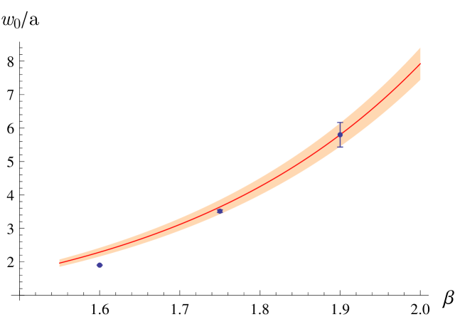
Figure 1: Scaling of $w_{0}$ compared to the expected behaviour from the $\beta$-function (red line). The orange band represents the statistical error determined by Eq. 7.

4 Matching the $\beta$-function

The Callan-Symanzik-$\beta$-function has been determined for the $\mathcal{N}=1$ SYM theory in Ref. [16] by instanton calculations. The result

$$\beta(g)=\mu\frac{d}{d\mu}g(\mu)=-\frac{g^{3}}{16\pi^{2}}\frac{3N_{c}}{1-\frac{N_{c}g^{2}}{8\pi^{2}}}$$ (6)

is exact due to the non-renormalisation theorem [16]. The first two perturbative coefficients are universal and scheme independent. The $\beta$-function can be used to compare lattice results at different bare gauge couplings $g$. If finite volume corrections and lattice discretisation errors can be neglected, the Wilson flow parameters $t_{0}$ and $w_{0}$ are expected to scale according to

$$\frac{w_{0}(g_{1})}{w_{0}(g_{2})}=\exp{(F(g_{1})-F(g_{2}))},$$ (7)

where the function $F(g)$ is the integral of the inverse of the $\beta$-function:

$$F(g)=\int^{g}\frac{dg^{\prime}}{\beta(g^{\prime})}=\frac{8\pi^{2}}{3N_{c}g^{2}}+\frac{2}{3}\ln g\,,$$ (8)

up to an unessential integration constant.

For our case, $N_{c}=2$, the scaling according to Eq. 7 has been checked by taking the value of $w_{0}$ at $\beta=4/g^{2}=1.9$ as reference point, see Fig. 1 . The agreement with Eq. 7 is rather good.

The relative deviation from the scaling,

$$K=\frac{w_{0}(1.9)}{w_{0}(\beta)}\left(\frac{1.9}{\beta}\right)^{1/3}\exp\left\{\frac{\pi^{2}(\beta-1.9)}{3}\right\},$$ (9)

is $K=1.03(6)$ for $\beta=1.75$ and $K=1.20(8)$ for $\beta=1.6$. The larger deviation at $\beta=1.6$ is presumably due to lattice artefacts and/or higher order terms in the lattice-$\beta$-function.

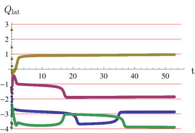
(a) $Q_{\textrm{lat}}(t)$

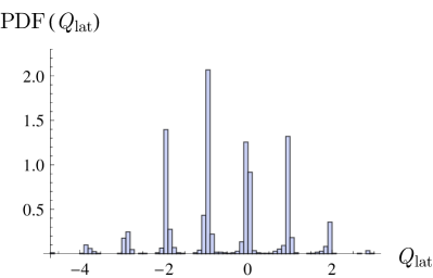
(b) PDF$(Q_{\textrm{lat}})$

Figure 2: (a) Topological charge for four different configuration as a function of the flow time $t$ on a $32^{3}\times 64$ lattice, $\beta=1.9$ and $\kappa=0.14435$. (b) Distribution of the topological charge at $t=50$ for the same run.

5 Measuring the topological charge with the Wilson flow

The topological charge is defined for a given field configuration in the continuum by the integral

$$Q_{\textrm{top}}=\frac{1}{32\pi^{2}}\int d^{4}x\,\epsilon_{\mu\nu\rho\sigma}F^{\mu\nu}_{a}F^{\rho\sigma}_{a}.$$ (10)

On the lattice we define the topological charge with the same antisymmetric discretisation of the field strength tensor as used for the flow equation:

$$Q_{\textrm{lat}}=\frac{1}{32\pi^{2}}\sum_{x}\epsilon_{\mu\nu\rho\sigma}G^{\mu\nu}_{a}G^{\rho\sigma}_{a}.$$ (11)

This lattice topological charge is affected by ultraviolet fluctuations, and its value is in general not an integer. A possible solution to this problem is a smoothing procedure to suppress the short distance fluctuations and to recover a well-defined topological charge in the continuum limit [17]. We have applied the Wilson flow as smoothing procedure, as done in Ref. [18].

As shown in Fig. 2(a), for large enough flow time $t$ the topological charge reaches a near integer value. Following Ref. [18], we convert the raw lattice topological charge to an integer using

$$Q_{\textrm{top}}=\textrm{round}{(\alpha Q_{\textrm{lat}}(t))},$$ (12)

where the flow time $t$ is chosen to be

$$t=\frac{1}{8}\left(\frac{L}{3}\right)^{2}$$ (13)

where $L$ is the spatial extent of the lattice. This value of $t$ is chosen sufficiently large to remove the cut-off effects; but not too large to change the number of instantons and the final value of the topological charge [19] . The real constant $\alpha$ is chosen to minimise the expectation value

$$R(\alpha)=\langle(\alpha Q_{\textrm{lat}}-\textrm{round}(\alpha Q_{\textrm{lat}}))^{2}\rangle.$$ (14)

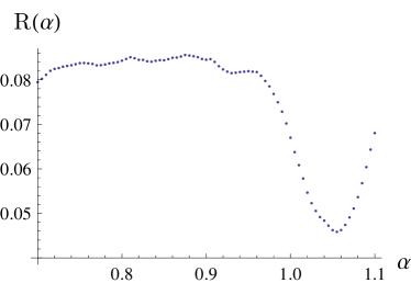
Figure 10: Plot of $R(\alpha)$ for the lattice $32^{3}\times 64$ at $\beta=1.75$ and $\kappa=0.1494$. The minimum of $R(\alpha)$ is located at $\alpha=1.055$.

Near the continuum limit it is expected that $\alpha\approx 1$, i.e. the distribution of $Q_{\textrm{lat}}$ is already centred near integer values without requiring an additional multiplicative renormalisation, see Fig. 2(b) (and Fig. 10 in the Appendix).

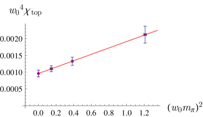
(a) $\chi_{\textrm{top}}$ at $\beta=1.60$

(b) $\chi_{\textrm{top}}$ at $\beta=1.75$

Figure 3: Extrapolation of the topological susceptibility $\chi_{\textrm{top}}$ to the chiral limit on a $32^{3}\times 64$ lattice at (a) $\beta=1.60$ and (b) $\beta=1.75$.

In addition, the topological susceptibility $\chi_{\textrm{top}}$, defined by

$$\chi_{\textrm{top}}=\frac{\langle Q_{\textrm{top}}^{2}\rangle-\langle Q_{\textrm{top}}\rangle^{2}}{V}\,=\frac{\langle Q_{\textrm{top}}^{2}\rangle-\langle Q_{\textrm{top}}\rangle^{2}}{a^{4}N_{s}^{3}N_{t}},$$ (15)

where $V$ is the volume of the system, has been measured. The results are shown in Tab. 2 and in Fig. 3. The value of $\chi_{\textrm{top}}$ extrapolated to the chiral limit confirms the topological suppression for SYM mentioned in Ref. [20].

6 Autocorrelation time of flow observables

The autocorrelation time of the topological charge increases drastically near the continuum limit and may even result in topological freezing. This effect depends, however, on the chosen boundary conditions [21, 22]. The scales $w_{0}$ and $t_{0}$ exhibit a very long autocorrelation time, especially near the continuum limit, similarly to the topological charge. Our configurations have been produced with the usual periodic boundary conditions and we observe the expected increase of the autocorrelations.

The autocorrelation time should scale with the lattice spacing $a$ asymptotically as $a^{-z}$, where $z=1$ for Hybrid Monte Carlo (HMC) algorithms. In our runs the lattice spacing is decreased roughly by a factor $2.5$ between $\beta=1.6$ and $\beta=1.9$. The integrated autocorrelation time $\tau(t_{0})$ of $t_{0}$ at $\beta=1.9$ is, however, approximately twelve times larger than at $\beta=1.6$, see Tab. 1.

Although the interval between $\beta=1.6$ and $\beta=1.9$ is presumably not yet in the asymptotic regime, the variation of $\tau(t_{0})$ seems to indicate a value $z\gtrsim 2$ and a possible connection of the topological charge with the flow observables used to set the scale.

7 Correlations between topological charge and the scale $w_{0}$

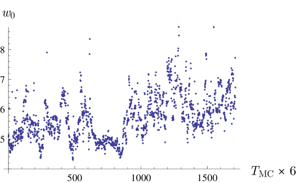
Figure 4: Monte Carlo history of $w_{0}$ on a $32^{3}\times 64$ lattice, $\beta=1.9$ and $\kappa=0.14435$. $T_{MC}$ is the Monte Carlo time. $w_{0}$ is measured every sixth configurations.

In order to investigate the nature of the long autocorrelation of $w_{0}$, we have considered its Monte Carlo history. The scale $w_{0}$ can be defined for a single configuration without the need of an ensemble average by determining the flow time when the integrated flow matches the condition specified by Eq. 5 . In Fig. 4 the Monte Carlo history of $w_{0}$ is shown for a lattice $32^{3}\times 64$ at $\beta=1.9$ and $\kappa=0.14435$. One can see that the value of $w_{0}$ has large fluctuations with a long period. In particular, very strong upward spikes emerge.

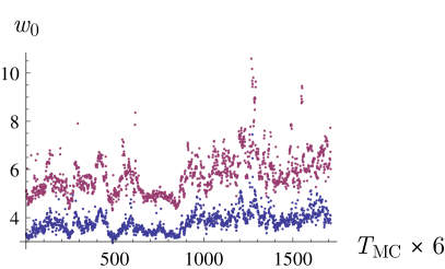
(a) $w_{0}^{0.1}$ versus $w_{0}^{0.3}$

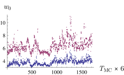
(b) $w_{0}^{0.1}$ versus $w_{0}^{0.4}$

Figure 5: Comparison of the Monte Carlo history (a) of $w_{0}^{0.1}$ (blue) with $w_{0}^{0.3}$ (red) and (b) of $w_{0}^{0.1}$ (blue) with $w_{0}^{0.4}$ (red), on a $32^{3}\times 64$ lattice, $\beta=1.9$ and $\kappa=0.14435$. The magnitude of the peaks increases drastically when the reference value to set the $w_{0}$ scale is larger.

Wilson flow scales depend implicitly on the reference value chosen in Eq. 5. Small reference values will potentially produce large lattice artefacts on the final results, while $w_{0}$ and $t_{0}$ will be affected by non-negligible finite volume effects for larger reference values. Let us define the scale $w_{0}^{u}$ to be the square root of the flow time when the condition

$$t\frac{d}{dt}t^{2}\langle E(t)\rangle=u$$ (16)

is satisfied. By varying $u$ one can study how the autocorrelations are affected by different choices of the reference value. Here and in the following we set $w_{0}\equiv w_{0}^{0.3}$. In Fig. 5 the Monte Carlo histories of $w_{0}^{0.1}$, $w_{0}^{0.3}$ and $w_{0}^{0.4}$ are compared. When the value of $u$ is small the fluctuations and spikes are significantly reduced. On the other hand, when the value of $u$ is increased the spikes become even more pronounced.

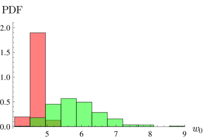
(a) Topological distribution of $w_{0}^{0.3}$

(b) Topological distribution of $w_{0}^{0.4}$

Figure 6: Probability distribution function of (a) $w_{0}^{0.3}$ and of (b) $w_{0}^{0.4}$ restricted to the topological sector $|Q_{\textrm{top}}|=1$ (green) and $|Q_{\textrm{top}}|=4$ (red) on a $32^{3}\times 64$ lattice, $\beta=1.9$ and $\kappa=0.14435$.

Increasing the value of $u$ leads to a larger flow time needed to match the condition (16), which means that a stronger smoothing induced by the flow equation is applied to the configurations. Large flow times will stronger remove ultraviolet fluctuations, and the system will be brought towards a classical configuration, as observed in section 5. Therefore one might argue that spikes and large fluctuations are related to topological effects. Using the results presented in section 5 we have been able to compute the value of $w_{0}^{u}$ restricted only to configurations with a fixed definite topological charge.

Figure 7: Linear fit of the dependence of $w_{0}^{u}$ on the topological charge for $u$ equal to 0.1 (green), 0.2 (yellow), 0.3 (purple) and 0.4 (blue) for a lattice $32^{3}\times 64$, $\beta=1.9$ and $\kappa=0.14435$.

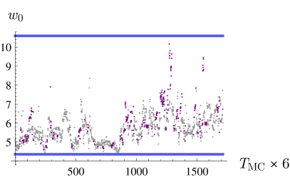
(a) Topological sector 0

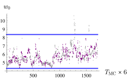
(b) Topological sector 1

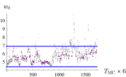
(c) Topological sector 2

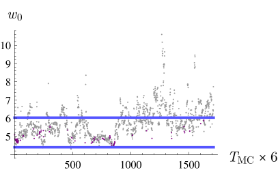
(d) Topological sector 3

Figure 11: Monte Carlo history of the $w_{0}$ on a $32^{3}\times 64$ lattice, $\beta=1.9$ and $\kappa=0.14435$. The purple points highlight the value of $w_{0}$ only for configurations characterised by a given topological sector; the blue lines mark its maximal and minimal value.

The distributions of $w_{0}^{0.4}$ and $w_{0}^{0.3}$ are shown for the same run in Fig. 6 for two selected topological sectors, $|Q_{\textrm{top}}|=1$ and $|Q_{\textrm{top}}|=4$. The distribution of $w_{0}^{0.3}$ restricted to the topological sector $|Q_{\textrm{top}}|=1$ is rather broad and the average value is larger than for the distribution in the topological sector $|Q_{\textrm{top}}|=4$. The same behaviour appears for the restricted distributions of $w_{0}^{0.4}$, but with a slightly larger difference between the two mean values of the distributions. This result clearly shows that there is a correlation between the value of $w_{0}$ and the topological charge, not only in terms of its mean value but also in terms of its distribution. The largest fluctuations observed in Fig. 4 are produced by the configurations at low values of the topological charge, where the distribution of $w_{0}$ is broad. The long periodicity is induced by the transitions during the Monte Carlo update time between topological sectors around zero, characterised by large expectation value of $w_{0}$, and topological sectors far from the origin with a small mean value of $w_{0}$. The Monte Carlo history restricted to a given topological sector is presented in Fig. 11 in the Appendix.

(a) $s$ versus $u$

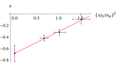
(b) $s$ versus $(w_{0}m_{\pi})^{2}$

Figure 8: (a) Slope coefficient $s$ as a function of the reference value $u$ for the lattice $32^{3}\times 64$, $\beta=1.9$ and $\kappa=0.14435$. (b) Slope coefficient $s$ as a function of $(w_{0}m_{\pi})^{2}$ at $\beta=1.9$ for $w_{0}^{0.3}$. The value of $s$ linearly extrapolated to the chiral limit is $s((w_{0}m_{\pi})^{2}=0)=-0.69(14)$.

In Fig. 7 we present the expectation value of $w_{0}^{u}$ restricted to the various topological sectors for four different values of $u$, in the same run on a $32^{3}\times 64$ lattice, with $\beta=1.9$ and $\kappa=0.14435$. The behaviour of $w_{0}^{u}(|Q_{\textrm{top}}|)$ is approximately linear for all $u$ but it has a steeper slope when the reference scale $u$ is larger. We have used a linear fit of the form

$$\langle w_{0}^{u}\rangle(|Q_{\textrm{top}}|)=s|Q_{\textrm{top}}|+q.$$ (17)

The resulting slope coefficients $s$ are presented as a function of $u$ in Fig. 8(a). The modulus of the slope $s$ increases increasing $u$. This means that the dependence of $w_{0}^{u}$ on the topology is stronger when $u$ is larger. This behaviour confirms our previous claim about the topological origin of the spikes in Fig. 5: when $u$ is large the smoothing effects of the Wilson flow are large and the configuration is driven towards a classical one where the influence of the topology is stronger. As a result, the integrated autocorrelation time of $w_{0}^{0.4}$ is around 800 $T_{MC}$, approximately three times larger than the autocorrelation time of $w_{0}^{0.1}$, which is around 300 $T_{MC}$. We have also investigated the dependence of $s$ on the adjoint pion mass squared, observing that it increases as one approaches the chiral limit, see Fig. 8(b).

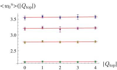
(a) $w_{0}^{u}(|Q_{\textrm{top}}|)$, lattice $32^{3}\times 64$

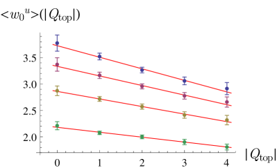
(b) $w_{0}^{u}(|Q_{\textrm{top}}|)$, lattice $16^{3}\times 36$

Figure 9: The same as Fig. 7, but for (a) the lattice $32^{3}\times 64$, $\beta=1.75$ and $\kappa=0.1494$; (b) the lattice $16^{3}\times 36$, $\beta=1.75$ and $\kappa=0.1490$.

The dependence of the flow scale on the topological charge can be interpreted as a finite volume effect [10, 11]. To address this point we repeated the same systematic analysis on the lattice $32^{3}\times 64$ at $\beta=1.75$, where the physical volume is approximately seven times larger than at $\beta=1.9$. The dependence of the various $w_{0}^{u}$ on $|Q_{\textrm{top}}|$ is presented in Fig. 9(a). As the figure shows, in this large physical volume the dependence of the flow scales on the topology completely disappears. If instead, the physical volume is shrunk again by simulating on a $16^{3}\times 36$ lattice at the same $\beta=1.75$, the observables $w_{0}^{u}$ appear to depend on the topological charge $|Q_{\textrm{top}}|$ as before, see Fig. 9(b). Note that the value of $\kappa$ used in the smaller volume is smaller than the first case, but according to Fig. 8(b) this should even reduce the slope. This demonstrates that finite volume effects are the origin of the dependence of $w_{0}$ on the topological charge in the runs on the finer lattices at $\beta=1.9$.

8 Conclusions

We have presented a detailed analysis of the Wilson flow observables $w_{0}$, used to set the scale alternatively to the Sommer parameter $r_{0}$. The same analysis has been done also for $t_{0}$ reaching similar conclusions. In finite volumes we observed a substantial dependence of $w_{0}$ on the topological charge, in agreement with the previous discussion on this topic for the Sommer parameter $r_{0}$ of Ref. [8, 9].

Scales based on the Wilson flow require a delicate fine-tuning to correctly handle finite volume effects and errors due to lattice artefacts. A result free of topological finite volume effects can be ensured if there is no coupling between the scale and the topological charge, up to the statistical precision. The final result has fairly small statistical and systematic errors, therefore $w_{0}$ can be used to set the scale in extrapolations to the chiral and to the continuum limit. Our observations support the use of small flow times to set the scale, at least for our model and within our present precision: the ratio of $w_{0}^{u}$ and $w_{0}^{0.3}$ is flat for $u\gtrsim 0.1$ (see Tab. 3 and Fig. 12 in the Appendix).

The results that have been presented may be different for other theories, in particular they may depend on the number of colours $N_{c}$, on the number of fermions $N_{f}$ and on the fermion representation. We believe, however, that a dependence of the scale on topology emerges for sufficient large reference scales independently of the theory. We therefore encourage systematic studies in this direction, in particular considering that there are proposals, like in [23], to increase the value of the reference flow time.

9 Acknowledgments

The authors gratefully acknowledge the Gauss Centre for Supercomputing (GCS) for providing computing time for a GCS Large Scale Project on the GCS share of the supercomputer JUQUEEN at Jülich Supercomputing Centre (JSC). GCS is the alliance of the three national supercomputing centres HLRS (Universität Stuttgart), JSC (Forschungszentrum Jülich), and LRZ (Bayerische Akademie der Wissenschaften), funded by the German Federal Ministry of Education and Research (BMBF) and the German State Ministries for Research of Baden-Württemberg (MWK), Bayern (StMWFK) and Nordrhein-Westfalen (MIWF).

Appendix A Tables and additional figures

Volume	$\beta$	$\kappa$	$am_{\pi}$	$\sqrt{t_{0}}/a$	$w_{0}/a$	$\tau({t_{0}})$
$24^{3}\times 48$	1.60	0.15500	0.5788(16)	1.5672(13)	1.5102(14)	21
$24^{3}\times 48$	1.60	0.15700	0.3264(23)	1.7904(11)	1.7292(37)	10
$24^{3}\times 48$	1.60	0.15750	0.2015(93)	1.8986(53)	1.8410(63)	42
$32^{3}\times 64$	1.75	0.14900	0.2385(4)	3.1438(67)	2.9838(59)	50
$32^{3}\times 64$	1.75	0.14920	0.2035(5)	3.270(17)	3.097(25)	45
$32^{3}\times 64$	1.75	0.14940	0.1604(15)	3.362(15)	3.205(20)	35
$32^{3}\times 64$	1.75	0.14950	0.1294(24)	3.551(36)	3.413(40)	65
$32^{3}\times 64$	1.90	0.14387	0.2123(4)	5.73(13)	5.57(19)	440
$32^{3}\times 64$	1.90	0.14415	0.1742(4)	5.71(12)	5.49(11)	296
$32^{3}\times 64$	1.90	0.14435	0.1413(6)	5.96(12)	5.76(14)	502

Table 1: Results for the adjoint pion mass $m_{\pi}$, the scales $t_{0}$, $w_{0}$ and the autocorrelation time $\tau({t_{0}})$ of $t_{0}$.

Run	Volume	$\beta$	$\kappa$	$(a^{4}\chi_{\textrm{top}})\times 10^{-6}$
A1	$24^{3}\times 48$	1.60	0.15500	160(19)
A2	$24^{3}\times 48$	1.60	0.15700	102(9)
A3	$24^{3}\times 48$	1.60	0.15750	85(7)
B1	$32^{3}\times 64$	1.75	0.14900	17(2)
B2	$32^{3}\times 64$	1.75	0.14920	12(1)
B3	$32^{3}\times 64$	1.75	0.14940	11(1)
B4	$32^{3}\times 64$	1.75	0.14950	10(3)
C1	$32^{3}\times 64$	1.90	0.14387	1.01(14)
C2	$32^{3}\times 64$	1.90	0.14415	1.59(18)
C3	$32^{3}\times 64$	1.90	0.14435	1.02(8)

Table 2: Results for the topological susceptibility.

Run	$w_{0}^{0.05}$	$w_{0}^{0.10}$	$w_{0}^{0.15}$	$w_{0}^{0.20}$	$w_{0}^{0.25}$	$w_{0}^{0.30}$	$w_{0}^{0.35}$	$w_{0}^{0.40}$
A1	0.6419(10)	0.9587(15)	1.1420(17)	1.2844(19)	1.4048(22)	1.5104(21)	1.6046(26)	1.6901(26)
A2	0.7767(15)	1.1136(22)	1.3192(27)	1.4787(34)	1.6122(40)	1.7290(43)	1.8319(46)	1.9268(44)
A3	0.8341(23)	1.1853(35)	1.4048(41)	1.5760(47)	1.7182(53)	1.8419(60)	1.9511(58)	2.0495(68)
B1	1.5087(42)	2.0058(51)	2.3331(56)	2.5878(60)	2.8011(62)	2.9838(59)	3.1495(62)	3.3012(62)
B2	1.5610(84)	2.082(15)	2.417(19)	2.684(19)	2.904(23)	3.097(25)	3.256(27)	3.424(25)
B3	1.6113(74)	2.151(12)	2.504(13)	2.779(17)	3.005(18)	3.205(20)	3.385(22)	3.551(25)
B4	1.6957(15)	2.269(24)	2.651(28)	2.955(34)	3.205(37)	3.413(41)	3.623(43)	3.793(42)
C1	2.734(46)	3.687(81)	4.35(10)	4.82(14)	5.24(16)	5.60(18)	5.90(18)	6.19(18)
C2	2.717(40)	3.666(85)	4.31(11)	4.76(13)	5.13(13)	5.49(13)	5.78(15)	6.05(14)
C3	2.855(44)	3.822(81)	4.47(11)	4.97(11)	5.40(14)	5.76(14)	6.08(15)	6.38(15)

Table 3: Results for the scale $w_{0}^{u}$.

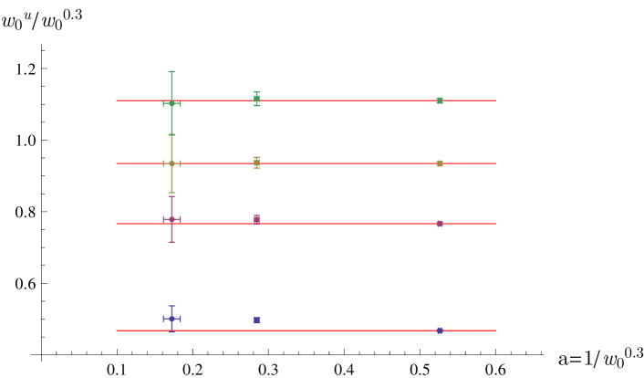
(a) $w_{0}^{u}/w_{0}^{0.3}$ for $u=0.05$ (blue), $u=0.15$ (purple), $u=0.25$ (yellow), $u=0.35$ (green).

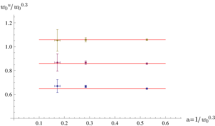
(b) $w_{0}^{u}/w_{0}^{0.3}$ for $u=0.10$ (blue), $u=0.20$ (purple), $u=0.40$ (yellow).

Figure 12: Scaling of the various $w_{0}^{u}$ with respect to $w_{0}^{0.3}$ as a function of the lattice spacing. The scaling is flat within the errors for $u\gtrsim 0.15$.

References

- [1] R. Sommer, Nucl. Phys. B 411 (1994) 839 [arXiv: hep-lat/9310022 ].
- [2] M. Lüscher, JHEP 1008 (2010) 071 [arXiv: 1006.4518 [hep-lat]].
-
[3]
R. Narayanan and H. Neuberger,
JHEP 0603 (2006) 064
[arXiv: hep-th/0601210 ]. - [4] S. Borsanyi et al., JHEP 1209 (2012) 010 [arXiv: 1203.4469 [hep-lat]].
- [5] G. Bergner, T. Berheide, I. Montvay, G. Münster, U. D. Özugurel and D. Sandbrink, JHEP 1209 (2012) 108 [arXiv: 1206.2341 [hep-lat]].
- [6] G. Bergner, I. Montvay, G. Münster, U. D. Özugurel and D. Sandbrink, JHEP 1311 (2013) 061 [arXiv: 1304.2168 [hep-lat]].
- [7] K. Demmouche, F. Farchioni, A. Ferling, I. Montvay, G. Münster, E.E. Scholz and J. Wuilloud, Eur. Phys. J. C 69 (2010) 147 [arXiv: 1003.2073 [hep-lat]].
- [8] F. Bruckmann, F. Gruber, K. Jansen, M. Marinkovic, C. Urbach and M. Wagner, Eur. Phys. J. A 43 (2010) 303 [arXiv: 0905.2849 [hep-lat]].
- [9] S. Aoki et al. [JLQCD Collaboration], Phys. Rev. D 78 (2008) 014508 [arXiv: 0803.3197 [hep-lat]].
- [10] R. Brower, S. Chandrasekharan, J.W. Negele and U.J. Wiese, Phys. Lett. B 560 (2003) 64 [arXiv: hep-lat/0302005 ].
- [11] S. Aoki, H. Fukaya, S. Hashimoto and T. Onogi, Phys. Rev. D 76 (2007) 054508 [arXiv: 0707.0396 [hep-lat]].
- [12] C. Morningstar and M.J. Peardon, Phys. Rev. D 69 (2004) 054501 [arXiv: hep-lat/0311018 ].
-
[13]
I. Montvay and E.E. Scholz,
Phys. Lett. B 623 (2005) 73
[arXiv: hep-lat/0506006 ]. -
[14]
E.E. Scholz and I. Montvay,
PoS(LAT2006) (2006) 037
[arXiv: hep-lat/0609042 ]. - [15] G. Münster and H. Stüwe, JHEP 1405 (2014) 034 [arXiv: 1402.6616 [hep-th]].
- [16] V.A. Novikov, M.A. Shifman, A.I. Vainshtein and V.I. Zakharov, Nucl. Phys. B 229 (1983) 381.
- [17] M. Creutz, Annals Phys. 326 (2011) 911 [arXiv: 1007.5502 [hep-lat]].
- [18] C. Bonati and M. D’Elia, Phys. Rev. D 89 (2014) 105005 [arXiv: 1401.2441 [hep-lat]].
- [19] D. A. Smith et al. [UKQCD Collaboration], Phys. Rev. D 58 (1998) 014505 [arXiv: hep-lat/9801008 ].
- [20] G. Bergner, P. Giudice, I. Montvay, G. Münster, U. D. Özugurel, S. Piemonte and D. Sandbrink, PoS(LATTICE2014) (2014) 273 [arXiv: 1411.1746 [hep-lat]].
- [21] M. Lüscher and S. Schaefer, JHEP 1107 (2011) 036 [arXiv: 1105.4749 [hep-lat]].
- [22] M. Lüscher and S. Schaefer, JHEP 1104 (2011) 104 [arXiv: 1103.1810 [hep-lat]].
- [23] R. Sommer, PoS(LATTICE 2013) (2014) 015 [arXiv: 1401.3270 [hep-lat]].