Polarized nonsinglet $\Delta q_{3}$ and nonsinglet fragmentation function $D^{\pi^{+}}_{u_{v}}$ in the analytic
approach to QCD

Abstract:

We discuss the application of an analytic approach called the analytic perturbation theory (APT) to the QCD analysis of DIS data. In particular, the results of the QCD analysis of a set of ‘fake’ data on the polarized nonsinglet $\Delta q_{3}$ and the nonsinglet fragmentation function $D^{\pi^{+}}_{u_{v}}$ by using the $Q^{2}$-evolution within the APT are considered. The ‘fake’ data are constructed based on parametrization of the polarized PDF and nonsinglet combination of the pion fragmentation functions. We confirm that APT can be successfully applied to QCD analysis of $\Delta q_{3}(x,Q^{2})$ and $D^{\pi^{+}}_{u_{v}}(z,Q^{2})$ and that the inequality $\Lambda_{\rm APT}>\Lambda_{\rm PT}$ obtained previously for the $xF_{3}(x)$ structure function takes place.

1 Introduction

We study the application of an analytic approach in QCD called the analytic perturbation theory (APT) [1] to the QCD analysis of deep inelastic scattering (DIS) data. The question is: how does the analytic approach work in comparison with the ordinary perturbation theory (PT)? Continuing our previous studies on the $F_{3}(x,Q^{2})$ structure function data [2, 3], we present the analysis in this direction for new physical quantities: polarized parton distribution functions (pdf’s) and fragmentation functions. We construct the so-called ‘fake’ data for the polarized nonsinglet combination $\Delta q_{3}(x,Q^{2})$ and nonsinglet fragmentation function $D^{\pi^{+}}_{u_{v}}(z,Q^{2})$, and compare the results of application of the PT and APT approaches in the analysis of these quantities. It should be noted that the application of the APT to QCD analysis of DIS data required a generalization of the analytic approach to the case of non-integer power of QCD running coupling. Such a generalization [4, 5], for example, was applied to analyze the $F_{2}(x,Q^{2})$ structure function behavior at small $x$-values [6, 7] and to analyze the low energy data on nucleon spin sum rules $\Gamma_{1}^{p,n}(Q^{2})$ [8].

2 Theoretical framework

In the leading order $(LO)$ we can write the APT nonsinglet moments $Q^{2}$ evolution as follows:

$${\cal{M}}^{\rm APT}(N,Q^{2})=\frac{{\cal{A}}_{\nu}(Q^{2})}{{\cal{A}}_{\nu}(Q_{0}^{2})}\,{\cal{M}}^{\rm APT}(N,Q^{2}_{0})\,,~{}~{}{\nu(N)}={{{\gamma_{NS}^{(0),N}}/{2\beta_{0}}}},~{}N=2,~{}3,...\,,$$ (1)

where the analytic function ${\cal{A}}_{\nu}$ is derived from the spectral representation and corresponds to the discontinuity of the $\nu$ power of the perturbative QCD coupling,  $\gamma_{NS}^{(0),N}$ are the nonsinglet one-loop anomalous dimensions, and $\beta_{0}=11-2n_{f}/3$.

The $LO$ expression for ${\cal{A}}_{\nu}$ has rather a simple analytic form [4] (see also Refs. [9, 10])

$${\cal{A}}_{\nu}(Q^{2}/\Lambda^{2})=\left[{a}_{\rm PT}\left({{Q^{2}}/{\Lambda^{2}}}\right)\right]^{\nu}\,-\,{{\rm{Li}_{1-\nu}}\left({\displaystyle\frac{\Lambda^{2}}{Q^{2}}}\right)}/{\Gamma(\nu)}\,,$$ (2)

where ${a}_{\rm PT}\equiv\beta_{0}\alpha_{\rm PT}/(4\pi)$ and ${\rm{Li}}_{\delta}(t)=\sum_{k=1}^{\infty}t^{k}/k^{\delta}$ is the polylogarithm function. The mathematical tool for numerical calculations of ${\cal{A}}_{\nu}$ for any $\nu\,$ up to four-loop order is given in Refs. [11, 12]. It should be stressed that values of the QCD scale parameter $\Lambda$ are different in the PT and APT approaches. The connection between $\Lambda_{{\rm PT}}$ and $\Lambda_{{\rm APT}}$ following from the condition $\left[{a}_{\rm PT}(Q^{2}/\Lambda^{2}_{{\rm PT}})\right]^{\nu}$ $={\cal{A}}_{\nu}(Q^{2}/\Lambda^{2}_{{\rm APT}})$ was given in Ref. [2]. From the previous QCD analysis for the $F_{3}(x,Q^{2})$ structure function data [3] it was obtained that

$$\Lambda_{{\rm APT}}>\Lambda_{{\rm PT}}.$$ (3)

A similar inequality was obtained from the analysis for the inclusive $\tau$ lepton into hadronic decays data (see, e.g., Refs. [13, 14]).

3 Fake data construction

3.1 Polarized nonsinglet $\Delta q_{3}$

We generate ‘fake’ data based on the results of the phenomenological analysis of polarized DIS data presented by Leader–Sidorov–Stamenov (LSS’10) [15], where the central values and corresponding uncertainties were presented for the parametrisation of polarised pdf’s. The kinematics region of the generated ‘fake’ data for the nonsinglet combination $x\Delta q_{3}(x,Q^{2})=[x\Delta u(x,Q^{2})+x\Delta{\bar{u}}(x,Q^{2})]-[x\Delta d(x,Q^{2})+x\Delta{\bar{d}}(x,Q^{2})]$ corresponds approximately to the those of the combined set of data used in Ref. [15]: $0.005<x<0.7$ and $1~{}{\mbox{\rm GeV}}^{2}<Q^{2}<65$ GeV², $4~{}{\mbox{\rm GeV}}^{2}<W^{2}$.

3.2 Nonsinglet $D^{\pi^{+}}_{u_{v}}(z,Q^{2})$

In the case of the nonsinglet valence combination $D^{\pi^{+}}_{u_{v}}(z,Q^{2})=D^{\pi^{+}}_{u}(z,Q^{2})-D^{\pi^{+}}_{\bar{u}}(z,Q^{2})$ the ‘fake’ data are generated based on the results of the LSS’14 [16] phenomenological analysis of multiplicities data of the HERMES collaboration [17]. The kinematics region of the generated ‘fake’ data for the nonsinglet combination $D^{\pi^{+}}_{u_{v}}(z,Q^{2})$ corresponds approximately to those of the HERMES pion multiplicities [17]: $0.2<z<0.7$ and $1.25~{}{\mbox{\rm GeV}}^{2}<Q^{2}<10$ GeV², $4~{}{\mbox{\rm GeV}}^{2}<W^{2}$. It should be noted that within the kinematics region of the multiplicities data of the HERMES collaboration analyzed in Ref. [16], the values of the quantity $t=-Q^{2}z/x\,$ [18] are not very large: $\mid{t}\mid\gtrsim 4.5~{}{\mbox{\rm GeV}}^{2}$.

4 Method of the QCD analysis

4.1 The PT $Q^{2}$ evolution

We follow the well-known approach based on the Jacobi polynomial expansion of structure functions. This method of solution of the Dokshitzer-Gribov-Lipatov-Altarelli-Parisi (DGLAP) evolution equation [19] was proposed in Ref. [20] and developed for both unpolarized [21] and polarized cases [22]. The main formula of this method allows an approximate reconstruction of the nonsinglet structure function through a finite number of Mellin moments. We’ll use the Jacobi method for the reconstruction of the polarized nonsinglet $\Delta q_{3}(x,Q^{2})$ and nonsinglet fragmentation function $D^{\pi^{+}}_{u_{v}}(z,Q^{2})$:

$$x\Delta q_{3}^{N_{max}}(x,Q^{2})=x^{\alpha}(1-x)^{\beta}\sum_{n=0}^{N_{max}}\Theta_{n}^{\alpha,\beta}(x)\sum_{j=0}^{n}c_{j}^{(n)}{(\alpha,\beta)}M_{j+2}(Q^{2})\,,$$ (4)

$$zD^{\pi^{+}N_{max}}_{u_{v}}(z,Q^{2})=z^{\alpha}(1-z)^{\beta}\sum_{n=0}^{N_{max}}\Theta_{n}^{\alpha,\beta}(z)\sum_{j=0}^{n}c_{j}^{(n)}{(\alpha,\beta)}M_{j+2}(Q^{2})\,.$$ (5)

Here $\Theta_{n}^{\alpha,\beta}$ are the Jacobi polynomials, $c_{j}^{(n)}(\alpha,\beta)$ contain $\alpha$- and $\beta$-dependent Euler $\Gamma$-functions where $\alpha,\beta$ are the Jacobi polynomial parameters fixed by the minimization of the error in the reconstruction of the function.

The perturbative renormalization group $Q^{2}$ evolution of moments is well known (see, e.g., [23]) and in the $LO$ reads as

$$~{}~{}~{}M^{pQCD}_{\rm i}(N,Q^{2})=\frac{~{}[a_{\rm PT}(Q^{2})]^{\nu}}{~{}[a_{\rm PT}(Q_{0}^{2})]^{\nu}}\,M_{\rm i}(N,Q^{2}_{0}),~{}~{}{\nu(N)}={{{\gamma_{NS}^{(0),N}}/{2\beta_{0}}}},~{}N=2,~{}3,...\,.$$ (6)

The unknown quantity ${M}_{\rm i}(N,Q^{2}_{0})$ could be parameterized as the Mellin moments of the functions $\Delta q_{3}(x,Q^{2})$ or $D^{\pi^{+}}_{u_{v}}(z,Q^{2})$ at some point, $Q^{2}_{0}$:

$${{M_{\Delta q_{3}}}}(N,Q^{2}_{0})=\int_{0}^{1}dx{x^{N-1}}x\Delta q_{3}(x,Q_{0}^{2})=\int_{0}^{1}dx{x^{N-2}}Ax^{a}(1-x)^{b}(1+\gamma x)\,,$$ (7)

$${{M_{D}}}(N,Q^{2}_{0})=\int_{0}^{1}dz{z^{N-1}}zD^{\pi^{+}}_{u_{v}}(z,Q_{0}^{2})=\int_{0}^{1}dz{z^{N-2}}Az^{a}(1-z)^{b}(1+\gamma z)\,.$$ (8)

The parameters $A$, $a$, $b$, $\gamma$ and the scale parameter $\Lambda_{QCD}$ are found by fitting a set of corresponding ‘fake’ data on $\Delta q_{3}(x,Q^{2})$ or $D^{\pi^{+}}_{u_{v}}(z,Q^{2})$, respectively. The detailed description of the fitting procedure could be found in Ref. [24].

4.2 The APT $Q^{2}$ evolution

In the framework of the analytical approach in QCD the expression for the Mellin moments evolution of the polarized nonsinglet $\Delta q_{3}$ and the nonsinglet valance combination of fragmentation functions $D^{\pi^{+}}_{u_{v}}$ is presented by Eq. (1). Similarly to the PT case, we can represented analytical moments at some point $Q^{2}_{0}$ in the following form:

$${{{\cal{M}}_{\Delta q_{3}}}}(N,Q^{2}_{0})=\int_{0}^{1}dx{x^{N-1}}x\Delta q_{3}(x,Q_{0}^{2})=\int_{0}^{1}dx{x^{N-2}}Ax^{a}(1-x)^{b}(1+\gamma x)\,,$$ (9)

$${{{\cal{M}}_{D}}}(N,Q^{2}_{0})=\int_{0}^{1}dz{z^{N-1}}zD^{\pi^{+}}_{u_{v}}(z,Q^{2}_{0})=\int_{0}^{1}dz{z^{N-2}}Az^{a}(1-z)^{b}(1+\gamma z)\,,$$ (10)

and expressions (4) and (5) are rewritten as

$$x\Delta q_{3}^{N_{max}}(x,Q^{2})=x^{\alpha}(1-x)^{\beta}\sum_{n=0}^{N_{max}}\Theta_{n}^{\alpha,\beta}(x)\sum_{j=0}^{n}c_{j}^{(n)}{(\alpha,\beta)}{\cal{M}}_{{\Delta q_{3}}}(j+2,Q^{2})\,,$$ (11)

$$zD^{\pi^{+}N_{max}}_{u_{v}}(z,Q^{2})=z^{\alpha}(1-z)^{\beta}\sum_{n=0}^{N_{max}}\Theta_{n}^{\alpha,\beta}(z)\sum_{j=0}^{n}c_{j}^{(n)}{(\alpha,\beta)}{\cal{M}}_{D}(j+2,Q^{2})\,.$$ (12)

As was mentioned above, the Jacobi method was applied to the QCD analysis in the polarized case in Ref. [22]. Here we apply this method in both the PT and APT approaches for reconstruction of the $Q^{2}$-evolution of polarized pdf’s and fragmentation functions.

5 Fitting results and discussion

The results of the $LO$ QCD fit of the ‘fake’ $\Delta q_{3}$ data in the PT and APT approaches are presented in Table 1 and Figs. 2 and 2. In both cases for the PT and APT, we put $Q^{2}_{0}=2$ GeV², number of active flavors $n_{f}=4$ and $N_{max}=11$. The value of errors of parameters correspond to $\Delta{\chi}^{2}=1$. One can be seen from Table 1 that values of the scale parameter $\Lambda$ are different in the PT and APT approaches and that $\Lambda_{\rm APT}>\Lambda_{\rm PT}$.

Table 1: The results for the QCD leading order fit of the ‘fake’ $\Delta q_{3}$ data in the standard PT and the APT approaches at $Q^{2}_{0}=2$ GeV², $Q^{2}>1$ GeV², $n_{f}=4$, and $N_{max}=11$.

	PT	APT
A	$0.807\pm 0.091$	$0.684\pm 0.052$
$\alpha$	$0.536\pm 0.024$	$0.505\pm 0.016$
$\beta$	$3.43\pm 0.023$	$3.56\pm 0.020$
$\gamma$	$9.89\pm 1.12$	$12.55\pm 0.87$
$\Lambda$ [MeV]	$256\pm 11$	$280\pm 15$

Figure 2 shows the $x\Delta q_{3}(x)$-shape obtained in the APT (solid line) and the PT (dotted line) cases. One can see that the result for the PT approach is slightly higher than for the APT one for large $x$-values. The difference $x\Delta q_{3}^{\rm PT}(x)-x\Delta q_{3}^{\rm APT}(x)$ vs. $x\,$ is more transparently shown on Fig. 2.

For the ‘fake’ data of the nonsinglet combination of the fragmentation functions $D^{\pi^{+}}_{u_{v}}(z,Q^{2})$ we have obtained a very similar shape for PT and APT approaches (see Fig. 3). The values of the scale parameter are: $\Lambda_{\rm APT}=307\pm 25$ MeV and $\Lambda_{\rm PT}=231\pm 12$ MeV.

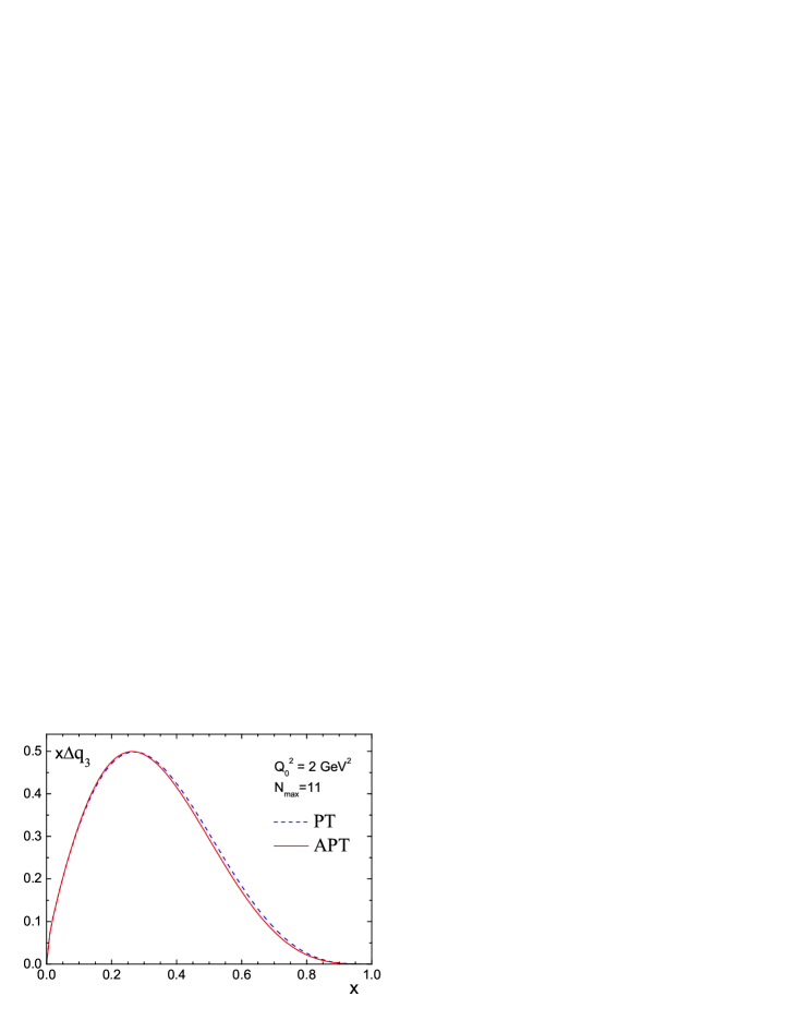
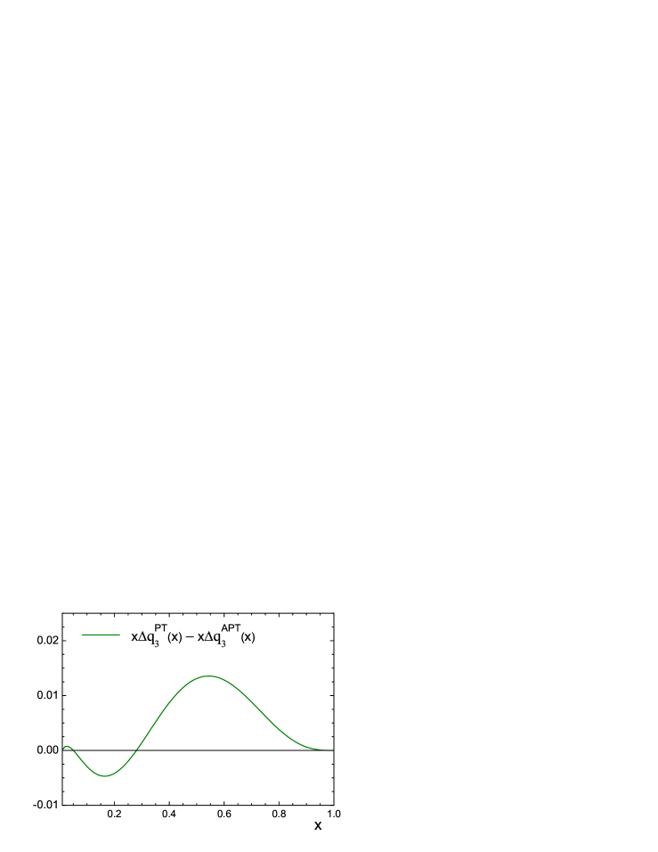
Figure 1: The $x{\Delta q}_{3}$-shape obtained in APT (solid line) and PT (dashed line).

          Figure 2: The difference in the PT and APT for the nonsinglet combination $x{\Delta q}_{3}(x)$.

Figure 3: The $D^{\pi^{+}}_{u_{v}}(z)$-shape obtained in APT (solid line) and PT (dashed line).

In general, for both nonsinglet combinations $x\Delta q_{3}(x)$ and $zD^{\pi^{+}}_{u_{v}}(z)$ the PT result is higher than for the APT one for large $x$ or $z$ respectively. The same property we have for $xF_{3}(x)$ structure function [3]. We confirm the inequality $\Lambda_{\rm APT}>\Lambda_{\rm PT}$, obtained previously for $xF_{3}(x)$ structure function.

It should be noted that kinematic area for variable $z$ is considerable narrower than the kinematic region for variable $x$. This may be the reason that the behavior of the $zD^{\pi^{+}}_{u_{v}}(z,Q^{2})$ function in the PT and APT approximations are practically the same (see Fig. 3).

References

• [1] D.V. Shirkov and I.L. Solovtsov, Phys. Rev. Lett. 79 (1997) 1209.
• [2] A.V. Sidorov and O.P. Solovtsova, Nonlin. Phenom. Complex Syst. 16 (2013) 397.
• [3] A.V. Sidorov and O.P. Solovtsova, Mod. Phys. Lett. A 29 (2014) 1450194, arXiv:1407.6858 [hep-ph].
• [4] A.P. Bakulev, S.V. Mikhailov and N.G. Stefanis, Phys. Rev. D 72 (2005) 074014; Erratum: ibid. D 72 (2005) 119908(E).
• [5] A.P. Bakulev, S.V. Mikhailov and N.G. Stefanis, Phys. Rev. D 75 (2007) 056005; Erratum: ibid. D 77 (2008) 079901(E).
• [6] G. Cvetic, A.Y. Illarionov, B.A. Kniehl and A.V. Kotikov, Phys. Lett. B 679 (2009) 350.
• [7] B.G. Shaikhatdenov, A.V. Kotikov, V.G. Krivokhizhin and G. Parente, Phys. Rev. D 81 (2010) 034008.
• [8] R.S. Pasechnik, D.V. Shirkov, O.V. Teryaev, O.P. Solovtsova and V.L. Khandramai, Phys. Rev. D 81 (2010) 016010.
• [9] G. Cvetic and A.V. Kotikov, J. Phys. G 39 (2012) 065005.
• [10] G. Cvetic, Phys. Rev. D 89 (2014) 036003.
• [11] A.P. Bakulev and V.L. Khandramai, Comput. Phys. Commun. 184 (2013) 183.
• [12] C. Ayala and G. Cvetic, “anQCD: a Mathematica package for calculations in general analytic QCD models,” arXiv:1408.6858 [hep-ph].
• [13] K.A. Milton, I.L. Solovtsov, O.P. Solovtsova and V.I. Yasnov, Eur. Phys. J. C 14 (2000) 495.
• [14] A.V. Nesterenko, “Dispersive approach to QCD: tau lepton hadronic decay in vector and axial-vector channels,” arXiv:1409.0687 [hep-ph].
• [15] E. Leader, A.V. Sidorov and D.B. Stamenov, Phys. Rev. D 82 (2010) 114018.
• [16] E. Leader, A.V. Sidorov and D.B. Stamenov, Phys. Rev. D 90 (2014) 054026.
• [17] A. Airapetain et al., Phys. Rev. D 87 (2013) 074029.
• [18] O.V. Teryaev, Acta Phys. Polon. B 33 (2002) 3749, arXiv:hep-ph/0211027.
• [19] V.N. Gribov and L.N. Lipatov, Sov. J. Nucl. Phys. 15 (1972) 438, Sov. J. Nucl. Phys. 15 (1972) 675;
G. Altarelli and G. Parisi, Nucl. Phys. B 126 (1977) 298;
Yu.L. Dokshitzer, Sov. Phys. JETP 46 (1977) 641.
• [20] G. Parisi and N. Sourlas, Nucl. Phys. B 151 (1979) 421;
I.S. Barker, C.B. Langensiepen and G. Shaw, Nucl. Phys. B 86 (1981) 61.
• [21] V.G. Krivokhizhin et al., Z. Phys. C 36 (1987) 51, Z. Phys. C 48 (1990) 347;
A. Benvenuti et al., Phys. Lett. B 195 (1987) 97, Phys. Lett. B 223 (1989) 490;
A.V. Kotikov, G. Parente and J. Sanchez-Guillen, Z. Phys. C 58 (1993) 465;
A.L. Kataev and A.V. Sidorov, Phys. Lett. B 331 (1994) 179.
• [22] E. Leader, A.V. Sidorov and D.B. Stamenov, Int. J. Mod. Phys. A 13 (1998) 5573;
Phys. Rev. D 58 (1998) 114028; C. Bourrely et al., Phys. Lett. B 442 (1998) 479.
• [23] A.J. Buras, Rev. Mod. Phys.  52 (1980) 199.
• [24] A.L. Kataev et al., Phys. Lett. B 417 (1998) 374.