Stochastic C-stability and B-consistency of explicit and implicit Euler-type schemes

Abstract.

This paper is concerned with the numerical approximation of stochastic ordinary differential equations, which satisfy a global monotonicity condition. This condition includes several equations with super-linearly growing drift and diffusion coefficient functions such as the stochastic Ginzburg-Landau equation and the 3/2-volatility model from mathematical finance. Our analysis of the mean-square error of convergence is based on a suitable generalization of the notions of C-stability and B-consistency known from deterministic numerical analysis for stiff ordinary differential equations. An important feature of our stability concept is that it does not rely on the availability of higher moment bounds of the numerical one-step scheme.

While the convergence theorem is derived in a somewhat more abstract framework, this paper also contains two more concrete examples of stochastically C-stable numerical one-step schemes: the split-step backward Euler method from Higham et al. (2002) and a newly proposed explicit variant of the Euler-Maruyama scheme, the so called projected Euler-Maruyama method. For both methods the optimal rate of strong convergence is proven theoretically and verified in a series of numerical experiments.

1. Introduction

Initiated by the papers [7] and [8] the field of numerical analysis for stochastic ordinary differential equations (SODEs) with super-linearly growing coefficient functions has seen a considerable progress, especially over the last couple of years. For instance, we refer to [10, 9, 12, 16, 21, 25] and the references therein.

The starting point of this article is the following observation: There exist strongly convergent numerical schemes, whose one-step maps satisfy suitable Lipschitz-type conditions, although the underlying stochastic differential equation has non-globally Lipschitz continuous coefficient functions. For the numerical approximation of stiff deterministic ODEs this observation has been formalized in the notion of C-stability, see for example [2, Definition 2.1.3] and [22, Chap. 8.4]. A related result is also found in [5, Prop. 15.2].

In this paper we present a generalization of this notion to the stochastic situation. Together with its counterpart, the notion of B-consistency, we will show that the error analysis of stochastically C-stable numerical methods can be simplified significantly compared to existing approaches in the literature. In particular, it turns out that it is not necessary to study higher moment estimates of the numerical scheme nor to consider their continuous time extensions.

We apply this more abstract framework to study the strong error of convergence for the numerical discretization of SODEs under the global monotonicity condition (see (3)). This condition includes several examples of SODEs with superlinearly growing drift and diffusion coefficient functions, for which the explicit Euler-Maruyama method is known to be divergent, see [11]. However, several explicit and implicit variants of the Euler-Maruyama method have been developed and analyzed in recent papers on this topic. For instance, we refer to [16] for the strong error analysis of the backward Euler method, and to [21, 25] for a corresponding result of the explicit tamed Euler method. Further, in [9] strong convergence rates are derived for a stopped-tamed Euler-Maruyama method applied to SODEs which lie beyond the global monotonicity condition.

In this paper we work with the following notion of strong convergence: We say that a numerical scheme converges strongly with order $\gamma$ to the exact solution $X\colon[0,T]\times\Omega\to{\mathbb{R}}^{d}$ if there exists a constant $C$ independent of the temporal step size $h$ such that

(1) $$\max_{n\in\{1,\ldots,N\}}\|X(t_{n})-X_{h}(t_{n})\|_{L^{2}(\Omega;{\mathbb{R}}^{d})}\leq C|h|^{\gamma}.$$

Here, $X_{h}\colon\{t_{0},t_{1},\ldots,t_{N}\}\times\Omega\to{\mathbb{R}}^{d}$ denotes the grid function generated by the numerical scheme. Let us remark that several of the above mentioned papers consider stronger notions of strong convergence, where, for example, the maximum occurs inside the $L^{2}$-norm or the norm in $L^{p}(\Omega;{\mathbb{R}}^{d})$ with $p>2$ is considered instead of the $L^{2}$-norm. Our choice of (1) is explained by the fact that our proof of the stability lemma (see Lemma 3.5), which plays a central role in our approach, relies on the orthogonality of the conditional expectation with respect to the norm in $L^{2}$.

In order to demonstrate the usefulness of our abstract results we present two more concrete examples of stochastically C-stable numerical schemes: First we are concerned with the split-step backward Euler method (SSBE) from [7], which is shown to be strongly convergent of order $\gamma=\frac{1}{2}$ in Theorem 5.8. Second, we propose a new explicit scheme, the projected Euler-Maruyama method (PEM), which turns out to be, in general, computationally less expensive then the implicit SSBE scheme. In Theorem 6.7 we verify that the PEM method is also strongly convergent of order $\frac{1}{2}$.

In our numerical experiments in Section 7 both methods perform equally well in terms of the experimental strong errors, which therefore indicates to favour the explicit PEM method due to its simpler implementation. However, this only holds true in the non-stiff case. As for deterministic ODEs, stiff problems may require an impractical small step size for an explicit numerical method while implicit schemes already give more useful results for larger step sizes, therefore reducing the overall computational cost. This is relevant if, for instance, the numerical one-step method is used for the time integration of a parabolic stochastic partial differential equation. Although we apply techniques from the numerical analysis of stiff equations in our error analyis we leave this issue to future research and concentrate here on non-stiff problems. In this context we also refer to [12] for a detailed comparison between implicit numerical methods and a further purely explicit variant of the Euler-Maruyama method, the tamed Euler method, which is considered in several of the above mentioned papers.

Let us briefly highlight two results in the literature, which are closely related to our approach from a methodological point of view: In [26] the authors investigate a family of one-leg theta methods for the discretization of SODEs under a one-sided Lipschitz condition on the drift and a global Lipschitz bound on the diffusion coefficient function. Hereby, they make use of the related notion of B-convergence. The second paper [25] presents a fundamental mean square convergence theorem for the discretization of SODEs under the global monotonicity condition. This theorem imposes a similar concept of the local truncation error as our notion of B-consistency. However, in the proof of the theorem the authors relate the global error at time $t_{i}$ to the error at time $t_{i-1}$ by one time step of the exact solution. Proceeding in this way one cannot benefit from the global Lipschitz properties of the numerical method.

The remainder of this paper is organized as follows: The following section contains a detailed description of the class of stochastic ordinary differential equations, whose solutions we want to approximate. Further, we state our main assumptions and present the numerical schemes, which are analyzed in the subsequent sections. In Section 3 we develop our notions of stochastic C-stability and B-consistency in a somewhat more abstract framework. Then we prove the already mentioned stability lemma, from which we easily deduce our strong convergence theorem for C-stable numerical methods.

In Section 4 we briefly summarize some results on the solvability of nonlinear equations, which are needed for the error analysis of the SSBE method. In Sections 5 and 6 we verify that the split-step backward Euler scheme and the projected Euler-Maruyama method are stochastically C-stable and B-consistent, and, hence, strongly convergent. In Section 7 we present some numerical experiments which illustrate our theoretical results for the discretization of the stochastic Ginzburg-Landau equation and for the financial $3/2$-volatility model.

2. Problem description and the numerical methods

In this section we introduce the class of stochastic differential equations, which we aim to discretize. Further, we state our main assumptions and the numerical methods, which we study in the remainder of this paper.

Let $d,m\in{\mathbb{N}}$, $T\in(0,\infty)$, and $(\Omega,{\mathcal{F}},({\mathcal{F}}_{t})_{t\in[0,T]},{\mathbf{P}})$ be a filtered probability space satisfying the usual conditions. We consider the solution $X\colon[0,T]\times\Omega\to{\mathbb{R}}^{d}$ to the SODE

(2) $$\begin{split}\,\mathrm{d}X(t)&=f(t,X(t))\,\mathrm{d}t+\sum_{r=1}^{m}g^{r}(t,X(t))\,\mathrm{d}W^{r}(t),\quad t\in[0,T],\\ X(0)&=X_{0}.\end{split}$$

Here $f\colon[0,T]\times{\mathbb{R}}^{d}\to{\mathbb{R}}^{d}$ stands for the drift coefficient function, while $g^{r}\colon[0,T]\times{\mathbb{R}}^{d}\to{\mathbb{R}}^{d}$, $r=1,\ldots,m$, are the diffusion coefficient functions. By $W^{r}\colon[0,T]\times\Omega\to{\mathbb{R}}$, $r=1,\ldots,m$, we denote an independent family of real-valued standard $({\mathcal{F}}_{t})_{t\in[0,T]}$-Brownian motions on $(\Omega,\mathcal{F},{\mathbf{P}})$. For a sufficiently large $p\in[2,\infty)$ the initial condition $X_{0}$ is assumed to be an element of the space $L^{p}(\Omega,{\mathcal{F}}_{0},{\mathbf{P}};{\mathbb{R}}^{d})$.

By $\langle\cdot,\cdot\rangle$ and $|\cdot|$ we denote the Euclidean inner product and the Euclidean norm on ${\mathbb{R}}^{d}$, respectively. Throughout this paper we impose the following conditions on the drift and the diffusion coefficient functions. Note that the strong convergence result for the SSBE method in Theorem 5.8 requires a more restrictive lower bound for the parameter $\eta$ appearing in (3).

Assumption 2.1.

The mappings $f\colon[0,T]\times{\mathbb{R}}^{d}\to{\mathbb{R}}^{d}$ and $g^{r}\colon[0,T]\times{\mathbb{R}}^{d}\to{\mathbb{R}}^{d}$, $r=1,\ldots,m$, are continuous. Furthermore, there exist a positive constant $L$ and a parameter value $\eta\in(\frac{1}{2},\infty)$ with

(3) $$\big{\langle}f(t,x_{1})-f(t,x_{2}),x_{1}-x_{2}\big{\rangle}+\eta\sum_{r=1}^{m}\big{|}g^{r}(t,x_{1})-g^{r}(t,x_{2})\big{|}^{2} \leq L|x_{1}-x_{2}|^{2}$$

for all $t\in[0,T]$ and $x_{1},x_{2}\in{\mathbb{R}}^{d}$. In addition, there exists a constant $q\in(1,\infty)$ such that for every $r=1,\ldots,m$ it holds

(4) $$|f(t,x)|\vee|g^{r}(t,x)| \leq L\big{(}1+|x|^{q}\big{)},$$

(5) $$|f(t_{1},x)-f(t_{2},x)|\vee|g^{r}(t_{1},x)-g^{r}(t_{2},x)| \leq L\big{(}1+|x|^{q}\big{)}|t_{1}-t_{2}|^{\frac{1}{2}},$$

(6) $$|f(t,x_{1})-f(t,x_{2})|\vee|g^{r}(t,x_{1})-g^{r}(t,x_{2})| \leq L\big{(}1+|x_{1}|^{q-1}+|x_{2}|^{q-1}\big{)}|x_{1}-x_{2}|,$$

for all $t,t_{1},t_{2}\in[0,T]$ and $x,x_{1},x_{2}\in{\mathbb{R}}^{d}$.

The assumption (3) is called global monotonicity condition. We exclude the case $q=1$, since this coincides with the well-known global Lipschitz case studied in [13, 17]. In Section 7 we present two more concrete SODEs, which fulfill Assumption 2.1.

Before we describe the numerical schemes we remark that Assumption 2.1 is also sufficient to ensure the existence of a unique solution to (2), see [14], [15, Chap. 2.3] or [20, Chap. 3]. By this we understand an almost surely continuous and $({\mathcal{F}}_{t})_{t\in[0,T]}$-adapted stochastic process $X\colon[0,T]\times\Omega\to{\mathbb{R}}^{d}$ which satisfies ${\mathbf{P}}$-almost surely the integral equation

(7) $$X(t)=X_{0}+\int_{0}^{t}f(s,X(s))\,\mathrm{d}s+\sum_{r=1}^{m}\int_{0}^{t}g^{r}(s,X(s))\,\mathrm{d}W^{r}(s)$$

for all $t\in[0,T]$. In addition, if there exist $C\in(0,\infty)$ and $p\in[2,\infty)$ such that

(8) $$\big{\langle}f(t,x),x\big{\rangle}+\frac{p-1}{2}\sum_{r=1}^{m}\big{|}g^{r}(t,x)\big{|}^{2} \leq C\big{(}1+|x|^{2}\big{)}$$

for all $x\in{\mathbb{R}}^{d}$, $t\in[0,T]$, then the exact solution has a finite $p$-th moment, that is

(9) $$\sup_{t\in[0,T]}\big{\|}X(t)\big{\|}_{L^{p}(\Omega;{\mathbb{R}}^{d})}<\infty.$$

For a proof we refer, for instance, to [15, Chap. 2.4]. The condition (8) is called global coercivity condition.

For the formulation of the numerical methods we introduce the following terminology: For $N\in{\mathbb{N}}$ we say that $h=(h_{1},\ldots,h_{N})\in(0,T]^{N}$ is a vector of (deterministic) step sizes if $\sum_{i=1}^{N}h_{i}=T$. Every vector of step sizes $h$ gives rise to a set of temporal grid points $\mathcal{T}_{h}$, which is given by

$$\mathcal{T}_{h}:=\Big{\{}t_{n}:=\sum_{i=1}^{n}h_{i}\,:\,n=0,\ldots,N\Big{\}}.$$

For short we write $|h|:=\max_{i\in\{1,\ldots,N\}}h_{i}$ for the maximal step size in $h$.

The aim of this paper is to show that the following two schemes are examples of stochastically C-stable numerical methods.

Example 2.2.

Consider the so called split-step backward Euler method (SSBE) studied in [7]. For its formulation let $h=(h_{1},\ldots,h_{N})$ be a vector of step sizes. Then the SSBE method is given by setting $X_{h}^{\mathrm{SSBE}}(0)=X_{0}$ and by the recursion

(10) $$\begin{split}\overline{X}_{h}^{\mathrm{SSBE}}(t_{i})&=X_{h}^{\mathrm{SSBE}}(t_{i-1})+h_{i}f(t_{i},\overline{X}_{h}^{\mathrm{SSBE}}(t_{i})),\\ X_{h}^{\mathrm{SSBE}}(t_{i})&=\overline{X}_{h}^{\mathrm{SSBE}}(t_{i})+\sum_{r=1}^{m}g^{r}(t_{i},\overline{X}_{h}^{\mathrm{SSBE}}(t_{i}))\big{(}W^{r}(t_{i})-W^{r}(t_{i-1})\big{)},\end{split}$$

for every $i=1,\ldots,N$. It is shown in Section 5 that the SSBE scheme is a well-defined stochastic one-step method under Assumption 2.1 and that it is strongly convergent of order $\gamma=\frac{1}{2}$, see Theorem 5.8.

Let us note that we evaluate the diffusion coefficient functions $g^{r}$ at time $t_{i}$ in the $i$-th step of the SSBE method. This is somewhat unusual when compared to the definition of the backward Euler scheme in [13, Chap. 12], where $g^{r}$ is evaluated at $t_{i-1}$ instead. The reason for this slight modification lies in condition (3), which is applied to $f$ and $g^{r}$, $r=1,\ldots,m$, simultaneously at the same point $t$ in time. Compare also with the inequality (21) further below. It helps to avoid some technical issues if we already take this relationship into consideration in the definition of the numerical scheme.

Example 2.3.

Another example of a stochastically C-stable scheme is the following explicit variant of the Euler-Maruyama method, which we term projected Euler-Maruyama method (PEM). It consists of the standard Euler-Maruyama method and a projection onto a ball in ${\mathbb{R}}^{d}$ whose radius is expanding with a negative power of the step size.

To be more precise, let $h\in(0,1]^{N}$ be an arbitrary vector of step sizes. The parameter value $\alpha\in(0,1]$ is chosen to be $\alpha=\frac{1}{2(q-1)}$ in dependence on the growth rate $q$ appearing in Assumption 2.1. Then, the PEM method is given by the recursion

(11) $$\begin{split}\overline{X}_{h}^{\mathrm{PEM}}(t_{i})&:=\min\big{(}1,h_{i}^{-\alpha}\big{|}X_{h}^{\mathrm{PEM}}(t_{i-1})\big{|}^{-1}\big{)}X_{h}^{\mathrm{PEM}}(t_{i-1}),\\ X_{h}^{\mathrm{PEM}}(t_{i})&:=\overline{X}_{h}^{\mathrm{PEM}}(t_{i})+h_{i}f(t_{i-1},\overline{X}_{h}^{\mathrm{PEM}}(t_{i}))\\ &\quad+\sum_{r=1}^{m}g^{r}(t_{i-1},\overline{X}_{h}^{\mathrm{PEM}}(t_{i}))\big{(}W^{r}(t_{i})-W^{r}(t_{i-1})\big{)},\;\text{ for }1\leq i\leq N,\end{split}$$

where $X_{h}^{\mathrm{PEM}}(0):=X_{0}$. The strong error analysis of the PEM method is carried out in Section 6.

To the best of our knowledge the PEM method for stochastic equations is new to the literature. Its definition is inspired by a truncation procedure, which plays an important role in the proof of [15, Chap. 2, Theorem 3.4]. For deterministic ODEs projection methods appear in geometric integration, see [4]. After the first preprint of this paper has appeared on arxiv.org the asymptotic stability and integrability property of a variant of the PEM method (11) is studied in [24] using Lyapunov function techniques.

3. An abstract convergence theorem

This section contains a detailed introduction to our notions of stochastic C-stability and B-consistency in a somewhat more abstract framework. Then we state our strong convergence theorem, whose proof turns out to be a direct application of the stability Lemma 3.5.

We begin by introducing some additional notation. By $\overline{h}\in(0,T]$ we denote an upper step size bound and we define the set $\mathbb{T}:=\mathbb{T}(\overline{h})\subset[0,T)\times(0,\overline{h}]$ to be

$$\mathbb{T}:=\big{\{}(t,\delta)\in[0,T)\times(0,\overline{h}]\,:\,t+\delta\leq T\big{\}}.$$

Further, for a given vector of step sizes $h\in(0,\overline{h}]^{N}$ we denote by $\mathcal{G}^{2}(\mathcal{T}_{h})$ the space of all adapted and square integrable grid functions, that is

$$\mathcal{G}^{2}(\mathcal{T}_{h}):=\big{\{}Z\colon\mathcal{T}_{h}\times\Omega\to{\mathbb{R}}^{d}\,:\,Z(t_{n})\in L^{2}(\Omega,{\mathcal{F}}_{t_{n}},{\mathbf{P}};{\mathbb{R}}^{d})\text{ for all }n=0,1,\ldots,N\big{\}}.$$

Our abstract class of stochastic one-step methods is defined as follows.

Definition 3.1.

Let $\overline{h}\in(0,T]$ be an upper step size bound and $\Psi\colon{\mathbb{R}}^{d}\times\mathbb{T}\times\Omega\to{\mathbb{R}}^{d}$ be a mapping satisfying the following measurability and integrability condition: For every $(t,\delta)\in\mathbb{T}$ and $Z\in L^{2}(\Omega,{\mathcal{F}}_{t},{\mathbf{P}};{\mathbb{R}}^{d})$ it holds

(12) $$\Psi(Z,t,\delta)\in L^{2}(\Omega,{\mathcal{F}}_{t+\delta},{\mathbf{P}};{\mathbb{R}}^{d}).$$

Then, for every vector of step sizes $h=(h_{1},\ldots,h_{N})\in(0,\overline{h}]^{N}$, $N\in{\mathbb{N}}$, we say that a grid function $X_{h}\in\mathcal{G}^{2}(\mathcal{T}_{h})$ is generated by the stochastic one-step method $(\Psi,\overline{h},\xi)$ with initial condition $\xi\in L^{2}(\Omega,{\mathcal{F}}_{0},{\mathbf{P}};{\mathbb{R}}^{d})$ if

(13) $$\begin{split}X_{h}(t_{i})&=\Psi(X_{h}(t_{i-1}),t_{i-1},h_{i}),\quad 1\leq i\leq N,\\ X_{h}(t_{0})&=\xi.\end{split}$$

We call $\Psi$ the one-step map of the method.

Next, we present our definition of stability for stochastic one-step methods. It is a suitable generalization of the notion of C-stability from [2, Definition 2.1.3] and has been used in the context of numerical approximation of stiff differential equations. We also refer to [5, Prop. 15.2] and to [22, Chap. 8.4] for a more recent exposition.

Definition 3.2.

A stochastic one-step method $(\Psi,\overline{h},\xi)$ is called stochastically C-stable (with respect to the norm in $L^{2}(\Omega;{\mathbb{R}}^{d})$) if there exist a constant $C_{\mathrm{stab}}$ and a parameter value $\eta\in(1,\infty)$ such that for all $(t,\delta)\in\mathbb{T}$ and all random variables $Y,Z\in L^{2}(\Omega,{\mathcal{F}}_{t},{\mathbf{P}};{\mathbb{R}}^{d})$ it holds

(14) $$\begin{split}&\big{\|}{\mathbb{E}}\big{[}\Psi(Y,t,\delta)-\Psi(Z,t,\delta)|{\mathcal{F}}_{t}\big{]}\big{\|}_{L^{2}(\Omega;{\mathbb{R}}^{d})}^{2}\\ &\qquad+\eta\big{\|}\big{(}\mathrm{id}-{\mathbb{E}}[\,\cdot\,|{\mathcal{F}}_{t}]\big{)}\big{(}\Psi(Y,t,\delta)-\Psi(Z,t,\delta)\big{)}\big{\|}^{2}_{L^{2}(\Omega;{\mathbb{R}}^{d})}\\ &\quad\leq\big{(}1+C_{\mathrm{stab}}\delta\big{)}\big{\|}Y-Z\big{\|}_{L^{2}(\Omega;{\mathbb{R}}^{d})}^{2}.\end{split}$$

Here and in what follows we denote by $\big{(}\mathrm{id}-{\mathbb{E}}[\,\cdot\,|{\mathcal{F}}_{t}]\big{)}Y=Y-{\mathbb{E}}[Y|{\mathcal{F}}_{t}]$ the projection of an ${\mathbb{R}}^{d}$-valued random variable orthogonal to the conditional expectation ${\mathbb{E}}[Y|{\mathcal{F}}_{t}]$. The next definition is concerned with the local truncation error. The conditions (15) and (16) are well-known in the literature and are found in slightly different form in [17, Th. 1.1] and [18, Th. 1.1]. A related concept has been applied in [25], but the authors need higher moment estimates of the local truncation error.

Definition 3.3.

A stochastic one-step method $(\Psi,\overline{h},\xi)$ is called stochastically B-consistent of order $\gamma>0$ to (2) if there exists a constant $C_{\mathrm{cons}}$ such that for every $(t,\delta)\in\mathbb{T}$ it holds

(15) $$\begin{split}\big{\|}{\mathbb{E}}\big{[}X(t+\delta)-\Psi(X(t),t,\delta)|{\mathcal{F}}_{t}\big{]}\big{\|}_{L^{2}(\Omega;{\mathbb{R}}^{d})}\leq C_{\mathrm{cons}}\delta^{\gamma+1}\end{split}$$

and

(16) $$\begin{split}\big{\|}\big{(}\mathrm{id}-{\mathbb{E}}[\,\cdot\,|{\mathcal{F}}_{t}]\big{)}\big{(}X(t+\delta)-\Psi(X(t),t,\delta)\big{)}\big{\|}_{L^{2}(\Omega;{\mathbb{R}}^{d})}\leq C_{\mathrm{cons}}\delta^{\gamma+\frac{1}{2}},\end{split}$$

where $X\colon[0,T]\times\Omega\to{\mathbb{R}}^{d}$ denotes the exact solution to (2).

Finally, it remains to give our definition of strong convergence.

Definition 3.4.

A stochastic one-step method $(\Psi,\overline{h},\xi)$ converges strongly with order $\gamma>0$ to the exact solution of (2) if there exists a constant $C$ such that for every vector of step sizes $h\in(0,\overline{h}]^{N}$ it holds

$$\max_{n\in\{0,\ldots,N\}}\big{\|}X_{h}(t_{n})-X(t_{n})\big{\|}_{L^{2}(\Omega;{\mathbb{R}}^{d})}\leq C|h|^{\gamma}.$$

Here $X$ denotes the exact solution to (2) and $X_{h}\in\mathcal{G}^{2}(\mathcal{T}_{h})$ is the grid function generated by $(\Psi,\overline{h},\xi)$ with step sizes $h\in(0,\overline{h}]^{N}$.

We first prove the following useful stability lemma. It follows from the discrete Gronwall Lemma and gives a motivation for the conditions (14) to (16). The underlying principle is similar to the proof of [17, Th. 1.1] and [18, Th. 1.1], but differs in one important point: In [17, Th. 1.1] the error at time $t_{i}$ is related to the error at time $t_{i-1}$ by one discrete time step of the exact solution (compare with [17, Lemma 1.1]). Here we follow the same idea, but we propagate the error by one application of the one-step map. This turns out to be important since a stochastically C-stable one-step method enjoys a global Lipschitz property.

Lemma 3.5.

Let $(\Psi,\overline{h},\xi)$ be a stochastically C-stable one-step method with constants $C_{\mathrm{stab}}$ and $\eta\in(1,\infty)$. Let $h\in(0,\overline{h}]^{N}$ be an arbitrary vector of step sizes. For every grid function $Z\in\mathcal{G}^{2}(\mathcal{T}_{h})$ it then follows that

$$\max_{n\in\{0,\ldots,N\}}\|Z(t_{n})-X_{h}(t_{n})\|_{L^{2}(\Omega;{\mathbb{R}}^{d})}^{2}\leq\mathrm{e}^{(1+C_{\mathrm{stab}}(1+\overline{h}))T}\Big{(}\|Z(0)-\xi\|_{L^{2}(\Omega;{\mathbb{R}}^{d})}^{2}$$

$$\qquad+\sum_{i=1}^{N}\big{(}1+h_{i}^{-1}\big{)}\big{\|}{\mathbb{E}}\big{[}Z(t_{i})-\Psi(Z(t_{i-1}),t_{i-1},h_{i})|{\mathcal{F}}_{t_{i-1}}\big{]}\big{\|}^{2}_{L^{2}(\Omega;{\mathbb{R}}^{d})}$$

$$\qquad+C_{\eta}\sum_{i=1}^{N}\big{\|}\big{(}\mathrm{id}-{\mathbb{E}}\big{[}\,\cdot\,|{\mathcal{F}}_{t_{i-1}}\big{]}\big{)}\big{(}Z(t_{i})-\Psi(Z(t_{i-1}),t_{i-1},h_{i})\big{)}\big{\|}^{2}_{L^{2}(\Omega;{\mathbb{R}}^{d})}\Big{)},$$

where $C_{\eta}=1+(\eta-1)^{-1}$ and $X_{h}\in\mathcal{G}^{2}(\mathcal{T}_{h})$ denotes the grid function generated by $(\Psi,\overline{h},\xi)$ with step sizes $h$.

Proof.

For every $1\leq i\leq N$ we write the difference of the two grid functions as

$$e_{h}(t_{i}) :=Z(t_{i})-X_{h}(t_{i}).$$

By the orthogonality of the conditional expectation it holds

$$\|e_{h}(t_{i})\|_{L^{2}(\Omega;{\mathbb{R}}^{d})}^{2}=\big{\|}{\mathbb{E}}[e_{h}(t_{i})|{\mathcal{F}}_{t_{i-1}}]\big{\|}^{2}_{L^{2}(\Omega;{\mathbb{R}}^{d})}+\big{\|}e_{h}(t_{i})-{\mathbb{E}}[e_{h}(t_{i})|{\mathcal{F}}_{t_{i-1}}]\big{\|}^{2}_{L^{2}(\Omega;{\mathbb{R}}^{d})}.$$

The first term is estimated as follows: Since

$$e_{h}(t_{i}) =Z(t_{i})-\Psi(Z(t_{i-1}),t_{i-1},h_{i})+\Psi(Z(t_{i-1}),t_{i-1},h_{i})-X_{h}(t_{i})$$

we first have

$$\big{\|}{\mathbb{E}}[e_{h}(t_{i})|{\mathcal{F}}_{t_{i-1}}]\big{\|}_{L^{2}(\Omega;{\mathbb{R}}^{d})} \leq\big{\|}{\mathbb{E}}\big{[}Z(t_{i})-\Psi(Z(t_{i-1}),t_{i-1},h_{i})|{\mathcal{F}}_{t_{i-1}}\big{]}\big{\|}_{L^{2}(\Omega;{\mathbb{R}}^{d})}$$

$$\quad+\big{\|}{\mathbb{E}}\big{[}\Psi(Z(t_{i-1}),t_{i-1},h_{i})-X_{h}(t_{i})|{\mathcal{F}}_{t_{i-1}}\big{]}\big{\|}_{L^{2}(\Omega;{\mathbb{R}}^{d})}.$$

Then, after taking squares, it follows from the inequality $(a+b)^{2}=a^{2}+2ab+b^{2}\leq(1+h_{i}^{-1})a^{2}+(1+h_{i})b^{2}$ that

$$\big{\|}{\mathbb{E}}[e_{h}(t_{i})|{\mathcal{F}}_{t_{i-1}}]\big{\|}^{2}_{L^{2}(\Omega;{\mathbb{R}}^{d})}$$

$$\quad\leq(1+h_{i}^{-1})\big{\|}{\mathbb{E}}\big{[}Z(t_{i})-\Psi(Z(t_{i-1}),t_{i-1},h_{i})|{\mathcal{F}}_{t_{i-1}}\big{]}\big{\|}_{L^{2}(\Omega;{\mathbb{R}}^{d})}^{2}$$

$$\qquad+(1+h_{i})\big{\|}{\mathbb{E}}\big{[}\Psi(Z(t_{i-1}),t_{i-1},h_{i})-X_{h}(t_{i})|{\mathcal{F}}_{t_{i-1}}\big{]}\big{\|}_{L^{2}(\Omega;{\mathbb{R}}^{d})}^{2}.$$

Replacing $h_{i}$ by $\eta-1$, the second term is estimated by

$$\big{\|}e_{h}(t_{i})-{\mathbb{E}}[e_{h}(t_{i})|{\mathcal{F}}_{t_{i-1}}]\big{\|}^{2}_{L^{2}(\Omega;{\mathbb{R}}^{d})}$$

$$\quad\leq C_{\eta}\big{\|}\big{(}\mathrm{id}-{\mathbb{E}}[\,\cdot\,|{\mathcal{F}}_{t_{i-1}}]\big{)}\big{(}Z(t_{i})-\Psi(Z(t_{i-1}),t_{i-1},h_{i})\big{)}\big{\|}^{2}_{L^{2}(\Omega;{\mathbb{R}}^{d})}$$

$$\qquad+\eta\big{\|}\big{(}\mathrm{id}-{\mathbb{E}}[\,\cdot\,|{\mathcal{F}}_{t_{i-1}}]\big{)}\big{(}\Psi(Z(t_{i-1}),t_{i-1},h_{i})-X_{h}(t_{i})\big{)}\big{\|}^{2}_{L^{2}(\Omega;{\mathbb{R}}^{d})},$$

where $C_{\eta}=1+(\eta-1)^{-1}$. To sum up, we have shown that

$$\big{\|}Z(t_{i})-X_{h}(t_{i})\big{\|}_{L^{2}(\Omega;{\mathbb{R}}^{d})}^{2}$$

$$\quad\leq(1+h_{i}^{-1})\big{\|}{\mathbb{E}}\big{[}Z(t_{i})-\Psi(Z(t_{i-1}),t_{i-1},h_{i})|{\mathcal{F}}_{t_{i-1}}\big{]}\big{\|}_{L^{2}(\Omega;{\mathbb{R}}^{d})}^{2}$$

$$\qquad+(1+h_{i})\big{\|}{\mathbb{E}}\big{[}\Psi(Z(t_{i-1}),t_{i-1},h_{i})-X_{h}(t_{i})|{\mathcal{F}}_{t_{i-1}}\big{]}\big{\|}_{L^{2}(\Omega;{\mathbb{R}}^{d})}^{2}$$

$$\qquad+C_{\eta}\big{\|}\big{(}\mathrm{id}-{\mathbb{E}}[\,\cdot\,|{\mathcal{F}}_{t_{i-1}}]\big{)}\big{(}Z(t_{i})-\Psi(Z(t_{i-1}),t_{i-1},h_{i})\big{)}\big{\|}^{2}_{L^{2}(\Omega;{\mathbb{R}}^{d})}$$

$$\qquad+\eta\big{\|}\big{(}\mathrm{id}-{\mathbb{E}}[\,\cdot\,|{\mathcal{F}}_{t_{i-1}}]\big{)}\big{(}\Psi(Z(t_{i-1}),t_{i-1},h_{i})-X_{h}(t_{i})\big{)}\big{\|}^{2}_{L^{2}(\Omega;{\mathbb{R}}^{d})}$$

for all $1\leq i\leq N$. After inserting $X_{h}(t_{i})=\Psi(X_{h}(t_{i-1}),t_{i-1},h_{i})$ and (14) we get

$$\big{\|}Z(t_{i})-X_{h}(t_{i})\big{\|}_{L^{2}(\Omega;{\mathbb{R}}^{d})}^{2}$$

$$\quad\leq(1+h_{i}^{-1})\big{\|}{\mathbb{E}}\big{[}Z(t_{i})-\Psi(Z(t_{i-1}),t_{i-1},h_{i})|{\mathcal{F}}_{t_{i-1}}\big{]}\big{\|}_{L^{2}(\Omega;{\mathbb{R}}^{d})}^{2}$$

$$\qquad+C_{\eta}\big{\|}\big{(}\mathrm{id}-{\mathbb{E}}[\,\cdot\,|{\mathcal{F}}_{t_{i-1}}]\big{)}\big{(}Z(t_{i})-\Psi(Z(t_{i-1}),t_{i-1},h_{i})\big{)}\big{\|}^{2}_{L^{2}(\Omega;{\mathbb{R}}^{d})}$$

$$\qquad+\big{(}1+(1+C_{\mathrm{stab}}(1+\overline{h}))h_{i}\big{)}\big{\|}Z(t_{i-1})-X_{h}(t_{i-1})\big{\|}_{L^{2}(\Omega;{\mathbb{R}}^{d})}^{2},$$

where we also made use of the fact that by (14)

$$h_{i}\big{\|}{\mathbb{E}}\big{[}\Psi(Z(t_{i-1}),t_{i-1},h_{i})-X_{h}(t_{i})|{\mathcal{F}}_{t_{i-1}}\big{]}\big{\|}_{L^{2}(\Omega;{\mathbb{R}}^{d})}^{2}$$

$$\quad\leq h_{i}(1+C_{\mathrm{stab}}\overline{h})\big{\|}Z(t_{i-1})-X_{h}(t_{i-1})\big{\|}_{L^{2}(\Omega;{\mathbb{R}}^{d})}^{2}.$$

Next, we subtract $\big{\|}Z(t_{i-1})-X_{h}(t_{i-1})\big{\|}_{L^{2}(\Omega;{\mathbb{R}}^{d})}^{2}$ from both sides of this inequality. Together with a telescopic sum argument this yields

$$\big{\|}Z(t_{n})-X_{h}(t_{n})\big{\|}_{L^{2}(\Omega;{\mathbb{R}}^{d})}^{2}-\big{\|}Z(0)-X_{h}(0)\big{\|}_{L^{2}(\Omega;{\mathbb{R}}^{d})}^{2}$$

$$\quad=\sum_{i=1}^{n}\Big{(}\big{\|}Z(t_{i})-X_{h}(t_{i})\big{\|}_{L^{2}(\Omega;{\mathbb{R}}^{d})}^{2}-\big{\|}Z(t_{i-1})-X_{h}(t_{i-1})\big{\|}_{L^{2}(\Omega;{\mathbb{R}}^{d})}^{2}\Big{)}$$

$$\quad\leq\sum_{i=1}^{n}\Big{(}\big{(}1+h_{i}^{-1}\big{)}\big{\|}{\mathbb{E}}\big{[}Z(t_{i})-\Psi(Z(t_{i-1}),t_{i-1},h_{i})|{\mathcal{F}}_{t_{i-1}}\big{]}\big{\|}^{2}_{L^{2}(\Omega;{\mathbb{R}}^{d})}$$

$$\qquad+C_{\eta}\big{\|}\big{(}\mathrm{id}-{\mathbb{E}}\big{[}\,\cdot\,|{\mathcal{F}}_{t_{i-1}}\big{]}\big{)}\big{(}Z(t_{i})-\Psi(Z(t_{i-1}),t_{i-1},h_{i})\big{)}\big{\|}^{2}_{L^{2}(\Omega;{\mathbb{R}}^{d})}$$

$$\qquad+(1+C_{\mathrm{stab}}(1+\overline{h}))h_{i}\big{\|}Z(t_{i-1})-X_{h}(t_{i-1})\big{\|}_{L^{2}(\Omega;{\mathbb{R}}^{d})}^{2}\Big{)}.$$

After adding $\|Z(0)-X_{h}(0)\|_{L^{2}(\Omega;{\mathbb{R}}^{d})}^{2}=\|Z(0)-\xi\|_{L^{2}(\Omega;{\mathbb{R}}^{d})}^{2}$ the assertion follows from an application of the discrete Gronwall Lemma. ∎

A simple consequence of the stability lemma is the following estimate of the second moment of the grid function generated by the numerical method.

Corollary 3.6.

Let $(\Psi,\overline{h},\xi)$ be stochastically C-stable. If there exists a constant $C_{0}$ such that for all $(t,\delta)\in\mathbb{T}$ it holds

$$\big{\|}{\mathbb{E}}\big{[}\Psi(0,t,\delta)|{\mathcal{F}}_{t}\big{]}\big{\|}_{L^{2}(\Omega;{\mathbb{R}}^{d})} \leq C_{0}\delta,$$

$$\big{\|}\big{(}\mathrm{id}-{\mathbb{E}}\big{[}\,\cdot\,|{\mathcal{F}}_{t}\big{]}\big{)}\Psi(0,t,\delta)\big{\|}_{L^{2}(\Omega;{\mathbb{R}}^{d})} \leq C_{0}\delta^{\frac{1}{2}},$$

then there exists a constant $C>0$ such that for all vectors of step sizes $h\in(0,\overline{h}]^{N}$,

$$\max_{n\in\{0,\ldots,N\}}\|X_{h}(t_{n})\|_{L^{2}(\Omega;{\mathbb{R}}^{d})}\leq\mathrm{e}^{CT}\Big{(}\|\xi\|_{L^{2}(\Omega;{\mathbb{R}}^{d})}^{2}+C_{0}^{2}(1+\overline{h}+C_{\eta})T\Big{)}^{\frac{1}{2}},$$

where $X_{h}$ denotes the grid function generated by $(\Psi,\overline{h},\xi)$ with step sizes $h$.

Proof.

The assertion follows directly from an application of Lemma 3.5 with $Z\equiv 0\in\mathcal{G}^{2}(\mathcal{T}_{h})$. ∎

As the next theorem shows consistency and stability imply the strong convergence of a stochastic one-step method.

Theorem 3.7.

Let the stochastic one-step method $(\Psi,\overline{h},\xi)$ be stochastically C-stable and stochastically B-consistent of order $\gamma>0$. If $\xi=X_{0}$, then there exists a constant $C$ depending on $C_{\mathrm{stab}}$, $C_{\mathrm{cons}}$, $T$, $\overline{h}$, and $\eta$ such that for every vector of step sizes $h\in(0,\overline{h}]^{N}$ it holds

$$\max_{n\in\{0,\ldots,N\}}\big{\|}X(t_{n})-X_{h}(t_{n})\big{\|}_{L^{2}(\Omega;{\mathbb{R}}^{d})}\leq C|h|^{\gamma},$$

where $X$ denotes the exact solution to (2) and $X_{h}$ the grid function generated by $(\Psi,\overline{h},\xi)$ with step sizes $h$. In particular, $(\Psi,\overline{h},\xi)$ is strongly convergent of order $\gamma$.

Proof.

Let $h\in(0,\overline{h}]^{N}$ be an arbitrary vector of step sizes. Since $X(0)=X_{h}(0)=X_{0}$ it directly follows from Lemma 3.5 that

$$\max_{n\in\{0,\ldots,N\}}\|X(t_{n})-X_{h}(t_{n})\|_{L^{2}(\Omega;{\mathbb{R}}^{d})}^{2}$$

$$\quad\leq\mathrm{e}^{(1+C_{\mathrm{stab}}(1+\overline{h}))T}\Big{(}\sum_{i=1}^{N}\big{(}1+h_{i}^{-1}\big{)}\big{\|}{\mathbb{E}}\big{[}X(t_{i})-\Psi(X(t_{i-1}),t_{i-1},h_{i})|{\mathcal{F}}_{t_{i}}\big{]}\big{\|}^{2}_{L^{2}(\Omega;{\mathbb{R}}^{d})}$$

$$\qquad+C_{\eta}\sum_{i=1}^{N}\big{\|}\big{(}\mathrm{id}-{\mathbb{E}}\big{[}\,\cdot\,|{\mathcal{F}}_{t_{i-1}}\big{]}\big{)}\big{(}X(t_{i})-\Psi(X(t_{i-1}),t_{i-1},h_{i})\big{)}\big{\|}^{2}_{L^{2}(\Omega;{\mathbb{R}}^{d})}\Big{)}.$$

After using (15) and (16) we get

$$\max_{n\in\{0,\ldots,N\}}\big{\|}X(t_{n})-X_{h}(t_{n})\big{\|}_{L^{2}(\Omega;{\mathbb{R}}^{d})}^{2}$$

$$\quad\leq\mathrm{e}^{(1+C_{\mathrm{stab}}(1+\overline{h}))T}C_{\mathrm{cons}}^{2}\sum_{i=1}^{N}\Big{(}(1+h_{i}^{-1})h_{i}^{2(\gamma+1)}+C_{\eta}h_{i}^{2\gamma+1}\Big{)}$$

$$\quad\leq\mathrm{e}^{(1+C_{\mathrm{stab}}(1+\overline{h}))T}(1+\overline{h}+C_{\eta})TC_{\mathrm{cons}}^{2}|h|^{2\gamma}.$$

This completes the proof. ∎

4. Solving nonlinear equations under a one-sided Lipschitz condition

This section collects some results on the solvability of nonlinear equations under a one-sided Lipschitz condition, which are needed for the error analysis of the split-step backward Euler scheme.

The following Uniform Monotonicity Theorem is a standard result in nonlinear analysis (see for instance, [19, Chap.6.4], [23, Theorem C.2]). We take explicit notice of the Lipschitz bound for the inverse which will be used later on.

Theorem 4.1.

Let $G\colon{\mathbb{R}}^{d}\to{\mathbb{R}}^{d}$ be a continuous mapping such that there exists a positive constant $c$ with

(17) $$\langle G(x_{1})-G(x_{2}),x_{1}-x_{2}\rangle\geq c|x_{1}-x_{2}|^{2}$$

for all $x_{1},x_{2}\in{\mathbb{R}}^{d}$. Then $G$ is a homeomorphism with Lipschitz continuous inverse, in particular

(18) $$\big{|}G^{-1}(y_{1})-G^{-1}(y_{2})\big{|}\leq\frac{1}{c}|y_{1}-y_{2}|$$

for all $y_{1},y_{2}\in{\mathbb{R}}^{d}$.

Proof.

It is well known [19, Chap. 6.4], [23, Theorem C.2] that $G(x)=y$ has a unique solution for every $y\in{\mathbb{R}}^{d}$. Setting $x_{1}=G^{-1}(y_{1}),x_{2}=G^{-1}(y_{2})$, condition (17) implies

$$c|x_{1}-x_{2}|^{2}\leq\langle y_{1}-y_{2},x_{1}-x_{2}\rangle\leq|y_{1}-y_{2}||x_{1}-x_{2}|,$$

from which the Lipschitz estimate (18) follows. ∎

The following consequence of Theorem 4.1 contains the key estimates for the C-stability of the split-step backward Euler scheme. For related estimates under global Lipschitz conditions on the diffusion coefficient functions we refer to [7, Lemmas 3.4, 4.5].

Corollary 4.2.

Let the functions $f\colon[0,T]\times{\mathbb{R}}^{d}\to{\mathbb{R}}^{d}$ and $g^{r}\colon[0,T]\times{\mathbb{R}}^{d}\to{\mathbb{R}}^{d}$, $r=1,\ldots,m$, satisfy Assumption 2.1 with Lipschitz constant $L>0$ and parameter value $\eta\in(\frac{1}{2},\infty)$. Let $\overline{h}\in(0,L^{-1})$ be given and define for every $\delta\in(0,\overline{h}]$ the mapping $F_{\delta}\colon[0,T]\times{\mathbb{R}}^{d}\to{\mathbb{R}}^{d}$ by $F_{\delta}(t,x)=x-\delta f(t,x)$. Then, the mapping ${\mathbb{R}}^{d}\ni x\mapsto F_{\delta}(t,x)\in{\mathbb{R}}^{d}$ is a homeomorphism for every $t\in[0,T]$.

In addition, the inverse $F_{\delta}^{-1}(t,\cdot)\colon{\mathbb{R}}^{d}\to{\mathbb{R}}^{d}$ satisfies

(19) $$\big{|}F_{\delta}^{-1}(t,x_{1})-F_{\delta}^{-1}(t,x_{2})\big{|} \leq(1-L\delta)^{-1}|x_{1}-x_{2}|,$$

(20) $$\big{|}F_{\delta}^{-1}(t,x)\big{|} \leq(1-L\delta)^{-1}\big{(}L\delta+|x|\big{)},$$

for every $x,x_{1},x_{2}\in{\mathbb{R}}^{d}$ and $t\in[0,T]$. Moreover, there exists a constant $C_{1}$ only depending on $L$ and $\overline{h}$ such that

(21) $$\begin{split}&\big{|}F_{\delta}^{-1}(t,x_{1})-F_{\delta}^{-1}(t,x_{2})\big{|}^{2}+\eta\delta\sum_{r=1}^{m}\big{|}g^{r}(t,F_{\delta}^{-1}(t,x_{1}))-g^{r}(t,F_{\delta}^{-1}(t,x_{2}))\big{|}^{2}\\ &\qquad\leq(1+C_{1}\delta)\big{|}x_{1}-x_{2}\big{|}^{2}\end{split}$$

for every $x_{1},x_{2}\in{\mathbb{R}}^{d}$ and $t\in[0,T]$.

Proof.

Fix arbitrary $\delta\in(0,\overline{h}]$ and $t\in[0,T]$. First, note that by (3) the mapping $F_{\delta}(t,\cdot)\colon{\mathbb{R}}^{d}\to{\mathbb{R}}^{d}$ is continuous and satisfies

$$\langle F_{\delta}(t,x_{1})-F_{\delta}(t,x_{2}),x_{1}-x_{2}\rangle$$

$$\quad=|x_{1}-x_{2}|^{2}-\delta\langle f(t,x_{1})-f(t,x_{2}),x_{1}-x_{2}\rangle\geq(1-L\delta)|x_{1}-x_{2}|^{2}$$

for all $x_{1},x_{2}\in{\mathbb{R}}^{d}$. Note that $1-L\delta>0$ follows from $\overline{h}\in(0,L^{-1})$ and $\delta\in(0,\overline{h}]$. Hence, we directly obtain the first assertion and (19) from Theorem 4.1.

Next, we set $x_{0}:=F_{\delta}(t,0)=-\delta f(t,0)\in{\mathbb{R}}^{d}$. Then $F_{\delta}^{-1}(t,x_{0})=0$ and for arbitrary $x\in{\mathbb{R}}^{d}$ by (19) and (4) we derive

$$\big{|}F_{\delta}^{-1}(t,x)\big{|} =\big{|}F_{\delta}^{-1}(t,x)-F_{\delta}^{-1}(t,x_{0})\big{|}\leq(1-L\delta)^{-1}|x-x_{0}|$$

$$\leq(1-L\delta)^{-1}\big{(}|x|+\delta|f(t,0)|\big{)}\leq(1-L\delta)^{-1}\big{(}|x|+L\delta\big{)}.$$

It remains to give a proof of (21). By also taking the diffusion coefficient functions into account, it follows from (3) that

$$\langle F_{\delta}(t,x_{1})-F_{\delta}(t,x_{2}),x_{1}-x_{2}\rangle$$

$$\quad=|x_{1}-x_{2}|^{2}-\delta\langle f(t,x_{1})-f(t,x_{2}),x_{1}-x_{2}\rangle$$

$$\quad\geq(1-L\delta)|x_{1}-x_{2}|^{2}+\eta\delta\sum_{r=1}^{m}\big{|}g^{r}(t,x_{1})-g^{r}(t,x_{2})\big{|}^{2}.$$

For some $y_{1},y_{2}\in{\mathbb{R}}^{d}$ we substitute $x_{1}=F_{\delta}^{-1}(t,y_{1})$ and $x_{2}=F_{\delta}^{-1}(t,y_{2})$ into the inequality. Then, after rearranging we end up with

$$\big{|}F_{\delta}^{-1}(t,y_{1})-F_{\delta}^{-1}(t,y_{2})\big{|}^{2}+\eta\delta\sum_{r=1}^{m}\big{|}g^{r}(t,F_{\delta}^{-1}(t,y_{1}))-g^{r}(t,F_{\delta}^{-1}(t,y_{2}))\big{|}^{2}$$

$$\quad\leq\big{\langle}y_{1}-y_{2},F_{\delta}^{-1}(t,y_{1})-F_{\delta}^{-1}(t,y_{2})\big{\rangle}+L\delta\big{|}F_{\delta}^{-1}(t,y_{1})-F_{\delta}^{-1}(t,y_{2})\big{|}^{2}.$$

Now, an application of (19), together with the Cauchy-Schwarz inequality, yields

$$\big{|}F_{\delta}^{-1}(t,y_{1})-F_{\delta}^{-1}(t,y_{2})\big{|}^{2}+\eta\delta\sum_{r=1}^{m}\big{|}g^{r}(t,F_{\delta}^{-1}(t,y_{1}))-g^{r}(t,F_{\delta}^{-1}(t,y_{2}))\big{|}^{2}$$

$$\quad\leq|y_{1}-y_{2}|\big{|}F_{\delta}^{-1}(t,y_{1})-F_{\delta}^{-1}(t,y_{2})\big{|}+L\delta\big{|}F_{\delta}^{-1}(t,y_{1})-F_{\delta}^{-1}(t,y_{2})\big{|}^{2}$$

$$\quad\leq(1-L\delta)^{-1}\big{(}1+(1-L\delta)^{-1}L\delta\big{)}|y_{1}-y_{2}|^{2}=(1-L\delta)^{-2}|y_{1}-y_{2}|^{2}$$

for all $y_{1},y_{2}\in{\mathbb{R}}^{d}$. Finally, note that $b(\delta)=(1-L\delta)^{-2}$ is a convex function, hence for all $\delta\in[0,\overline{h}]$,

$$(1-L\delta)^{-2}\leq 1+C_{1}\delta,\quad C_{1}=\frac{b(\overline{h})-b(0)}{\overline{h}}=L(2-L\overline{h})(1-L\overline{h})^{-2},$$

and inequality (21) is verified. ∎

The following lemma contains some further estimates of $F_{\delta}^{-1}$, which will be useful for the analysis of the local truncation error.

Lemma 4.3.

Consider the same situation as in Corollary 4.2. Then there exist constants $C_{2}$, $C_{3}$ only depending on $L$, $\overline{h}$ and $q$ such that for every $\delta\in(0,\overline{h}]$ the inverse $F_{\delta}^{-1}(t,\cdot)\colon{\mathbb{R}}^{d}\to{\mathbb{R}}^{d}$ satisfies the estimates

(22) $$\big{|}F_{\delta}^{-1}(t,x)-x\big{|} \leq\delta C_{2}\big{(}1+|x|^{q}\big{)},$$

(23) $$\big{|}F_{\delta}^{-1}(t,x)-x-\delta f(t,x)\big{|} \leq\delta^{2}C_{3}\big{(}1+|x|^{2q-1}\big{)}$$

for every $x\in{\mathbb{R}}^{d}$ and $t\in[0,T]$.

Proof.

Let $x\in{\mathbb{R}}^{d}$ be arbitrary. For the proof of (22) we get from (19) that

$$\big{|}F_{\delta}^{-1}(t,x)-x\big{|}=\big{|}F_{\delta}^{-1}(t,x)-F_{\delta}^{-1}(t,F_{\delta}(t,x))\big{|}\leq(1-L\delta)^{-1}\delta\big{|}f(t,x)\big{|}.$$

After inserting (4) and since $\delta\leq\overline{h}$ we arrive at

$$\big{|}F_{\delta}^{-1}(t,x)-x\big{|}\leq L(1-L\overline{h})^{-1}\delta\big{(}1+|x|^{q}\big{)},$$

which is (22) with $C_{2}=L(1-L\overline{h})^{-1}$.

Next, by making use of the substitution $y=F_{\delta}^{-1}(t,x)$ as well as (6) we obtain

$$\big{|}F_{\delta}^{-1}(t,x)-x-\delta f(t,x)\big{|}=\big{|}y-F_{\delta}(t,y)-\delta f(t,F_{\delta}(t,y))\big{|}$$

$$\quad=\delta\big{|}f(t,y)-f(t,F_{\delta}(t,y))\big{|}$$

$$\quad\leq L\delta\big{(}1+|y|^{q-1}+|F_{\delta}(t,y)|^{q-1}\big{)}\big{|}y-F_{\delta}(t,y)\big{|}$$

$$\quad\leq L\delta\big{(}1+|x|^{q-1}+|F_{\delta}^{-1}(t,x)|^{q-1}\big{)}\big{|}F_{\delta}^{-1}(t,x)-x\big{|}$$

for every $x\in{\mathbb{R}}^{d}$. After inserting (22) and (20) we find that

$$\big{|}F_{\delta}^{-1}(t,x)-x-\delta f(t,x)\big{|} \leq C_{2}L\delta^{2}\big{(}1+|x|^{q}\big{)}\big{(}1+|x|^{q-1}+|F_{\delta}^{-1}(t,x)|^{q-1}\big{)}$$

$$\leq\delta^{2}C_{3}\big{(}1+|x|^{2q-1}\big{)}$$

for a suitable constant $C_{3}$ only depending on $q$, $L$, and $\overline{h}$. ∎

5. C-stability and B-consistency of the SSBE method

In Section 3 we derived a strong convergence result in an abstract framework. Using Section 4 we are now able to verify that the split-step backward Euler scheme from Example 2.2 is stable and consistent with order $\gamma=\frac{1}{2}$.

Let us first show that the SSBE method is indeed a well-defined stochastic one-step method in the sense of Definition 3.1. In Section 4 we saw that the implicit step of the SSBE method admits a unique solution if $f$ satisfies Assumption 2.1 with one-sided Lipschitz constant $L$. To be more precise, let $\overline{h}\in(0,L^{-1})$ and consider an arbitrary vector of step sizes $h\in(0,\overline{h}]^{N}$. Then, we obtain from Corollary 4.2 that for every $1\leq i\leq N$ there exists a homeomorphism $F_{h_{i}}(t_{i},\cdot)\colon{\mathbb{R}}^{d}\to{\mathbb{R}}^{d}$ such that $\overline{X}_{h}^{\mathrm{SSBE}}(t_{i})=F_{h_{i}}^{-1}(t_{i},X_{h}^{\mathrm{SSBE}}(t_{i-1}))$ is the solution to

$$\overline{X}_{h}^{\mathrm{SSBE}}(t_{i}) =X_{h}^{\mathrm{SSBE}}(t_{i-1})+h_{i}f(t_{i},\overline{X}_{h}^{\mathrm{SSBE}}(t_{i})).$$

Hence, we define the one-step map $\Psi^{\mathrm{SSBE}}\colon{\mathbb{R}}^{d}\times\mathbb{T}\times\Omega\to{\mathbb{R}}^{d}$ of the split-step backward Euler method by

(24) $$\Psi^{\mathrm{SSBE}}(x,t,\delta)=F_{\delta}^{-1}(t+\delta,x)+\sum_{r=1}^{m}g^{r}(t+\delta,F_{\delta}^{-1}(t+\delta,x))\Delta_{\delta}W^{r}(t)$$

for every $x\in{\mathbb{R}}^{d}$ and $(t,\delta)\in\mathbb{T}$, where $\Delta_{\delta}W^{r}(t):=W^{r}(t+\delta)-W^{r}(t)$. Next, we verify that $\Psi^{\mathrm{SSBE}}$ satisfies condition (12) and the assumptions of Corollary 3.6.

Proposition 5.1.

Let the functions $f$ and $g^{r}$, $r=1,\ldots,m$, satisfy Assumption 2.1 with $L\in(0,\infty)$ and $q\in(1,\infty)$ and let $\overline{h}\in(0,L^{-1})$. For every initial value $\xi\in L^{2}(\Omega;{\mathcal{F}}_{0},{\mathbf{P}};{\mathbb{R}}^{d})$ it holds that $(\Psi^{\mathrm{SSBE}},\overline{h},\xi)$ is a stochastic one-step method.

In addition, there exists a constant $C_{0}$, which depends on $L$, $q$, $m$, and $\overline{h}$, such that

(25) $$\big{\|}{\mathbb{E}}\big{[}\Psi^{\mathrm{SSBE}}(0,t,\delta)|{\mathcal{F}}_{t}\big{]}\big{\|}_{L^{2}(\Omega;{\mathbb{R}}^{d})} \leq C_{0}\delta,$$

(26) $$\big{\|}\big{(}\mathrm{id}-{\mathbb{E}}[\,\cdot\,|{\mathcal{F}}_{t}]\big{)}\Psi^{\mathrm{SSBE}}(0,t,\delta)\big{\|}_{L^{2}(\Omega;{\mathbb{R}}^{d})} \leq C_{0}\delta^{\frac{1}{2}}$$

for all $(t,\delta)\in\mathbb{T}$.

Proof.

For the first assertion we only have to verify that $\Psi^{\mathrm{SSBE}}$ satisfies (12). For this we fix arbitrary $(t,\delta)\in\mathbb{T}$ and $Z\in L^{2}(\Omega,{\mathcal{F}}_{t},{\mathbf{P}};{\mathbb{R}}^{d})$. Then, we obtain from Corollary 4.2 that the mapping $F_{\delta}^{-1}(t+\delta,\cdot)\colon{\mathbb{R}}^{d}\to{\mathbb{R}}^{d}$ is a homeomorphism satisfying the linear growth bound (20). Hence, we have

$$F_{\delta}^{-1}(t+\delta,Z)\in L^{2}(\Omega,{\mathcal{F}}_{t},{\mathbf{P}};{\mathbb{R}}^{d}).$$

Consequently, by the continuity of $g^{r}$ the mapping

$$\Omega\ni\omega\mapsto g^{r}(t+\delta,F_{\delta}^{-1}(t+\delta,Z(\omega)))\in{\mathbb{R}}^{d}$$

is ${\mathcal{F}}_{t}/{\mathcal{B}}({\mathbb{R}}^{d})$-measurable for every $r=1,\ldots,m$. Therefore, $\Psi^{\mathrm{SSBE}}(Z,t,\delta)\colon\Omega\to{\mathbb{R}}^{d}$ is a well-defined random variable, which is ${\mathcal{F}}_{t+\delta}/{\mathcal{B}}({\mathbb{R}}^{d})$-measurable. It remains to show that $\Psi^{\mathrm{SSBE}}(Z,t,\delta)$ is square integrable.

For this we first consider the case that $Z=0\in L^{2}(\Omega;{\mathbb{R}}^{d})$. Then it is evident that $\Psi^{\mathrm{SSBE}}(0,t,\delta)\in L^{2}(\Omega,{\mathcal{F}}_{t+\delta},{\mathbf{P}};{\mathbb{R}}^{d})$. In particular, it follows from (20) that

$$\big{\|}{\mathbb{E}}\big{[}\Psi^{\mathrm{SSBE}}(0,t,\delta)|{\mathcal{F}}_{t}\big{]}\big{\|}_{L^{2}(\Omega;{\mathbb{R}}^{d})}=\big{|}F_{\delta}^{-1}(t+\delta,0)\big{|}\leq(1-L\delta)^{-1}L\delta\leq(1-L\overline{h})^{-1}L\delta.$$

Further, from an application of Itō’s isometry, (4) and (20) we get

$$\big{\|}\big{(}\mathrm{id}-{\mathbb{E}}[\,\cdot\,|{\mathcal{F}}_{t}]\big{)}\Psi^{\mathrm{SSBE}}(0,t,\delta)\big{\|}_{L^{2}(\Omega;{\mathbb{R}}^{d})}^{2}$$

$$\quad=\Big{\|}\sum_{r=1}^{m}g^{r}(t+\delta,F_{\delta}^{-1}(t+\delta,0))\big{(}W^{r}(t+\delta)-W^{r}(t)\big{)}\Big{\|}^{2}_{L^{2}(\Omega;{\mathbb{R}}^{d})}$$

$$\quad=\delta\sum_{r=1}^{m}\big{|}g^{r}(t+\delta,F_{\delta}^{-1}(t+\delta,0))\big{|}^{2}$$

$$\quad\leq L^{2}m\delta\big{(}1+\big{|}F_{\delta}^{-1}(t+\delta,0)\big{|}^{q}\big{)}^{2}\leq L^{2}m\big{(}1+(1-L\overline{h})^{-q}L^{q}\overline{h}^{q}\big{)}^{2}\delta.$$

This verifies (25) and (26).

Next, for arbitrary $Z\in L^{2}(\Omega;{\mathcal{F}}_{t},{\mathbf{P}};{\mathbb{R}}^{d})$ we compute by similar arguments

$$\big{\|}\Psi^{\mathrm{SSBE}}(Z,t,\delta)-\Psi^{\mathrm{SSBE}}(0,t,\delta)\big{\|}^{2}_{L^{2}(\Omega;{\mathbb{R}}^{d})}$$

$$\quad=\big{\|}F_{\delta}^{-1}(t+\delta,Z)-F_{\delta}^{-1}(t+\delta,0)\big{\|}_{L^{2}(\Omega;{\mathbb{R}}^{d})}^{2}$$

$$\qquad+\delta\sum_{r=1}^{m}\big{\|}g^{r}(t+\delta,F_{\delta}^{-1}(t+\delta,Z))-g^{r}(t+\delta,F_{\delta}^{-1}(t+\delta,0))\big{\|}_{L^{2}(\Omega;{\mathbb{R}}^{d})}^{2}$$

$$\quad={\mathbb{E}}\Big{[}\big{|}F_{\delta}^{-1}(t+\delta,Z)-F_{\delta}^{-1}(t+\delta,0)\big{|}^{2}$$

$$\qquad+\delta\sum_{r=1}^{m}\big{|}g^{r}(t+\delta,F_{\delta}^{-1}(t+\delta,Z))-g^{r}(t+\delta,F_{\delta}^{-1}(t+\delta,0))\big{|}^{2}\Big{]}.$$

Thus, an application of (21) yields

$$\big{\|}\Psi^{\mathrm{SSBE}}(Z,t,\delta)-\Psi^{\mathrm{SSBE}}(0,t,\delta)\big{\|}^{2}_{L^{2}(\Omega;{\mathbb{R}}^{d})}\leq(1+C_{1}\delta)\|Z\|^{2}_{L^{2}(\Omega;{\mathbb{R}}^{d})}.$$

This completes the proof. ∎

Theorem 5.2.

Let the functions $f$ and $g^{r}$, $r=1,\ldots,m$, satisfy Assumption 2.1 with $L\in(0,\infty)$ and $\eta\in(1,\infty)$. Further, let $\overline{h}\in(0,L^{-1})$. Then, for every $\xi\in L^{2}(\Omega,{\mathcal{F}}_{0},{\mathbf{P}};{\mathbb{R}}^{d})$ the SSBE scheme $(\Psi^{\mathrm{SSBE}},\overline{h},\xi)$ is stochastically C-stable.

Proof.

Let us consider arbitrary $(t,\delta)\in\mathbb{T}$ and $Y,Z\in L^{2}(\Omega,{\mathcal{F}}_{t},{\mathbf{P}};{\mathbb{R}}^{d})$. For the proof of (14) we first note that

$${\mathbb{E}}\big{[}\Psi^{\mathrm{SSBE}}(Y,t,\delta)-\Psi^{\mathrm{SSBE}}(Z,t,\delta)|{\mathcal{F}}_{t}\big{]}=F_{\delta}^{-1}(t+\delta,Y)-F_{\delta}^{-1}(t+\delta,Z)$$

and

$$\big{(}\mathrm{id}-{\mathbb{E}}[\,\cdot\,|{\mathcal{F}}_{t}]\big{)}\big{(}\Psi^{\mathrm{SSBE}}(Y,t,\delta)-\Psi^{\mathrm{SSBE}}(Z,t,\delta)\big{)}$$

$$\quad=\sum_{r=1}^{m}\big{(}g^{r}(t+\delta,F_{\delta}^{-1}(t+\delta,Y))-g^{r}(t+\delta,F_{\delta}^{-1}(t+\delta,Z))\big{)}\Delta_{\delta}W^{r}(t).$$

Then we obtain from (21)

$$\big{\|}F_{\delta}^{-1}(t+\delta,Y)-F_{\delta}^{-1}(t+\delta,Z)\big{\|}_{L^{2}(\Omega;{\mathbb{R}}^{d})}^{2}$$

$$\quad+\eta\Big{\|}\sum_{r=1}^{m}\big{(}g^{r}(t+\delta,F_{\delta}^{-1}(t+\delta,Y))-g^{r}(t+\delta,F_{\delta}^{-1}(t+\delta,Z))\big{)}\Delta_{\delta}W^{r}(t)\Big{\|}^{2}_{L^{2}(\Omega;{\mathbb{R}}^{d})}$$

$$={\mathbb{E}}\Big{[}\big{|}F_{\delta}^{-1}(t+\delta,Y)-F_{\delta}^{-1}(t+\delta,Z)\big{|}^{2}$$

$$\qquad+\eta\delta\sum_{r=1}^{m}\big{|}g^{r}(t+\delta,F_{\delta}^{-1}(t+\delta,Y))-g^{r}(t+\delta,F_{\delta}^{-1}(t+\delta,Z))\big{|}^{2}\Big{]}$$

$$\leq(1+C_{1}\delta)\big{\|}Y-Z\big{\|}^{2}_{L^{2}(\Omega;{\mathbb{R}}^{d})}.$$

which is condition (14) for the SSBE method with $C_{\mathrm{stab}}=C_{1}$. ∎

The following fact is a consequence of Theorem 5.2 and Corollary 3.6 together with (25) and (26).

Corollary 5.3.

Let the functions $f$ and $g^{r}$, $r=1,\ldots,m$, satisfy Assumption 2.1 with $L\in(0,\infty)$ and $\eta\in(1,\infty)$. Let $\overline{h}\in(0,L^{-1})$. Then, for every vector of step sizes $h\in(0,\overline{h}]^{N}$ it holds for the grid function $X_{h}$ generated by $(\Psi^{\mathrm{SSBE}},\overline{h},\xi)$ that

$$\max_{n\in\{0,\ldots,N\}}\|X_{h}^{\mathrm{SSBE}}(t_{n})\|_{L^{2}(\Omega;{\mathbb{R}}^{d})}\leq\mathrm{e}^{CT}\Big{(}\|\xi\|^{2}_{L^{2}(\Omega;{\mathbb{R}}^{d})}+C_{0}^{2}(1+\overline{h}+C_{\eta})T\Big{)}^{\frac{1}{2}},$$

where the constant $C_{0}$ is the same as in Proposition 5.1.

In preparation of the proof of consistency we state the following result on the Hölder continuity of the exact solution to (2) with respect to the norm in $L^{p}(\Omega;{\mathbb{R}}^{d})$.

Proposition 5.4.

Let $f$ and $g^{r}$, $r=1,\ldots,m$, satisfy Assumption 2.1 with $L\in(0,\infty)$ and $q\in(1,\infty)$. For every $p\in[2,\infty)$ with $\sup_{t\in[0,T]}\|X(t)\|_{L^{pq}(\Omega;{\mathbb{R}}^{d})}<\infty$ there exists a constant $C$ such that

$$\big{\|}X(t_{1})-X(t_{2})\big{\|}_{L^{p}(\Omega;{\mathbb{R}}^{d})}\leq C\big{(}1+\sup_{t\in[0,T]}\|X(t)\|_{L^{pq}(\Omega;{\mathbb{R}}^{d})}^{q}\big{)}|t_{1}-t_{2}|^{\frac{1}{2}}$$

for all $t_{1},t_{2}\in[0,T]$, where $X$ denotes the exact solution to (2).

Proof.

Let $0\leq t_{1}<t_{2}\leq T$. After inserting (7) we get

$$\big{\|}X(t_{1})-X(t_{2})\big{\|}_{L^{p}(\Omega;{\mathbb{R}}^{d})} \leq\int_{t_{1}}^{t_{2}}\big{\|}f(\tau,X(\tau))\big{\|}_{L^{p}(\Omega;{\mathbb{R}}^{d})}\,\mathrm{d}\tau$$

$$\quad+\Big{\|}\sum_{r=1}^{m}\int_{t_{1}}^{t_{2}}g^{r}(\tau,X(\tau))\,\mathrm{d}W^{r}(\tau)\Big{\|}_{L^{p}(\Omega;{\mathbb{R}}^{d})}.$$

For the drift integral it follows from (4) that

$$\int_{t_{1}}^{t_{2}}\big{\|}f(\tau,X(\tau))\big{\|}_{L^{p}(\Omega;{\mathbb{R}}^{d})}\,\mathrm{d}\tau\leq L\big{(}1+\sup_{\tau\in[0,T]}\|X(\tau)\|_{L^{pq}(\Omega;{\mathbb{R}}^{d})}^{q}\big{)}|t_{1}-t_{2}|.$$

In addition, the Burkholder-Davis-Gundy inequality yields

$$\Big{\|}\sum_{r=1}^{m}\int_{t_{1}}^{t_{2}}g^{r}(\tau,X(\tau))\,\mathrm{d}W^{r}(\tau)\Big{\|}_{L^{p}(\Omega;{\mathbb{R}}^{d})}\leq C\Big{(}\sum_{r=1}^{m}\int_{t_{1}}^{t_{2}}\big{\|}g^{r}(\tau,X(\tau))\big{\|}^{2}_{L^{p}(\Omega;{\mathbb{R}}^{d})}\,\mathrm{d}\tau\Big{)}^{\frac{1}{2}}$$

for a constant $C=C(p)$. Then, we deduce from (4) that

$$\big{\|}g^{r}(\tau,X(\tau))\big{\|}_{L^{p}(\Omega;{\mathbb{R}}^{d})}\leq L\big{(}1+\sup_{\tau\in[0,T]}\big{\|}X(\tau)\big{\|}_{L^{pq}(\Omega;{\mathbb{R}}^{d})}^{q}\big{)}.$$

Therefore, it holds

$$\Big{\|}\sum_{r=1}^{m}\int_{t_{1}}^{t_{2}}g^{r}(\tau,X(\tau))\,\mathrm{d}W^{r}(\tau)\Big{\|}_{L^{p}(\Omega;{\mathbb{R}}^{d})}$$

$$\quad\leq CLm^{\frac{1}{2}}\big{(}1+\sup_{\tau\in[0,T]}\big{\|}X(\tau)\big{\|}_{L^{pq}(\Omega;{\mathbb{R}}^{d})}^{q}\big{)}|t_{1}-t_{2}|^{\frac{1}{2}}.$$

This completes the proof. ∎

The following two lemmas contain estimates, which play important roles in the proofs of consistency for the SSBE scheme and the PEM method.

Lemma 5.5.

Let Assumption 2.1 be satisfied by $f$ and $g^{r}$, $r=1,\ldots,m$, with $L\in(0,\infty)$ and $q\in(1,\infty)$. Further, let the exact solution $X$ to (2) satisfy $\sup_{t\in[0,T]}\|X(t)\|_{L^{4q-2}(\Omega;{\mathbb{R}}^{d})}<\infty$. Then, there exists a constant $C$ such that for all $t_{1},t_{2}\in[0,T]$ and $s_{1},s_{2}\in[t_{1},t_{2}]$ it holds

$$\int_{t_{1}}^{t_{2}}\big{\|}f(\tau,X(\tau))-f(s_{1},X(s_{2}))\big{\|}_{L^{2}(\Omega;{\mathbb{R}}^{d})}\,\mathrm{d}\tau$$

$$\quad\leq C\big{(}1+\sup_{t\in[0,T]}\big{\|}X(t)\big{\|}_{L^{4q-2}(\Omega;{\mathbb{R}}^{d})}^{2q-1}\big{)}|t_{1}-t_{2}|^{\frac{3}{2}}.$$

Proof.

It follows from (5) and (6) that

$$\big{|}f(\tau_{1},x_{1})-f(\tau_{2},x_{2})\big{|} \leq\big{|}f(\tau_{1},x_{1})-f(\tau_{1},x_{2})\big{|}+\big{|}f(\tau_{1},x_{2})-f(\tau_{2},x_{2})\big{|}$$

$$\leq L\big{(}1+|x_{1}|^{q-1}+|x_{2}|^{q-1}\big{)}|x_{1}-x_{2}|+L\big{(}1+|x_{2}|^{q}\big{)}|\tau_{1}-\tau_{2}|^{\frac{1}{2}}$$

for all $\tau_{1},\tau_{2}\in[0,T]$ and $x_{1},x_{2}\in{\mathbb{R}}^{d}$. By an additional application of Hölder’s inequality with exponents $\rho=2-\frac{1}{q}$ and $\rho^{\prime}=\frac{2q-1}{q-1}$ we get for all $s_{1},s_{2},\tau\in[t_{1},t_{2}]$

(27) $$\begin{split}&\big{\|}f(\tau,X(\tau))-f(s_{1},X(s_{2}))\big{\|}_{L^{2}(\Omega;{\mathbb{R}}^{d})}\\ &\quad\leq L\big{\|}\big{(}1+|X(\tau)|^{q-1}+|X(s_{2})|^{q-1}\big{)}|X(\tau)-X(s_{2})|\big{\|}_{L^{2}(\Omega;{\mathbb{R}})}\\ &\qquad+L\big{\|}\big{(}1+|X(s_{2})|^{q}\big{)}|\tau-s_{1}|^{\frac{1}{2}}\big{\|}_{L^{2}(\Omega;{\mathbb{R}}^{d})}\\ &\quad\leq L\big{(}1+2\sup_{t\in[0,T]}\|X(t)\|^{q-1}_{L^{2\rho^{\prime}(q-1)}(\Omega;{\mathbb{R}}^{d})}\big{)}\|X(\tau)-X(s_{2})\|_{L^{2\rho}(\Omega;{\mathbb{R}}^{d})}\\ &\qquad+L\big{(}1+\sup_{t\in[0,T]}\|X(t)\|^{q}_{L^{2q}(\Omega;{\mathbb{R}}^{d})}\big{)}|t_{1}-t_{2}|^{\frac{1}{2}}.\end{split}$$

Observe that $2\rho^{\prime}(q-1)=4q-2$ and $2q\leq 4q-2$ for $q\in(1,\infty)$. Moreover, Proposition 5.4 with $p=2\rho$ yields

$$\|X(\tau)-X(s_{2})\|_{L^{2\rho}(\Omega;{\mathbb{R}}^{d})} \leq C\big{(}1+\sup_{t\in[0,T]}\|X(t)\|_{L^{2\rho q}(\Omega;{\mathbb{R}}^{d})}^{q}\big{)}|\tau-s_{2}|^{\frac{1}{2}}$$

$$\leq C\big{(}1+\sup_{t\in[0,T]}\|X(t)\|_{L^{4q-2}(\Omega;{\mathbb{R}}^{d})}^{q}\big{)}|t_{1}-t_{2}|^{\frac{1}{2}}.$$

Altogether, this proves

$$\big{\|}f(\tau,X(\tau))-f(s_{1},X(s_{2}))\big{\|}_{L^{2}(\Omega;{\mathbb{R}}^{d})}\leq C\big{(}1+\sup_{t\in[0,T]}\|X(t)\|_{L^{4q-2}(\Omega;{\mathbb{R}}^{d})}^{2q-1}\big{)}|t_{1}-t_{2}|^{\frac{1}{2}}$$

for all $s_{1},s_{2},\tau\in[t_{1},t_{2}]$. After integrating over $\tau\in[t_{1},t_{2}]$ the proof is completed. ∎

Lemma 5.6.

Let Assumption 2.1 be satisfied by $f$ and $g^{r}$, $r=1,\ldots,m$. Further, let the exact solution $X$ to (2) satisfy $\sup_{\tau\in[0,T]}\|X(\tau)\|_{L^{4q-2}(\Omega;{\mathbb{R}}^{d})}<\infty$. Then, there exists a constant $C$ such that for all $t_{1},t_{2},s\in[0,T]$ with $0\leq t_{1}\leq s\leq t_{2}\leq T$ it holds

$$\Big{\|}\sum_{r=1}^{m}\int_{t_{1}}^{t_{2}}\big{(}g^{r}(\tau,X(\tau))-g^{r}(s,X(t_{1}))\big{)}\,\mathrm{d}W^{r}(\tau)\Big{\|}_{L^{2}(\Omega;{\mathbb{R}}^{d})}$$

$$\quad\leq Cm^{\frac{1}{2}}\big{(}1+\sup_{\tau\in[0,T]}\big{\|}X(\tau)\big{\|}_{L^{4q-2}(\Omega;{\mathbb{R}}^{d})}^{2q-1}\big{)}|t_{1}-t_{2}|.$$

Proof.

By the Itō isometry we get

$$\Big{\|}\sum_{r=1}^{m}\int_{t_{1}}^{t_{2}}\big{(}g^{r}(\tau,X(\tau))-g^{r}(s,X(t_{1}))\big{)}\,\mathrm{d}W^{r}(\tau)\Big{\|}_{L^{2}(\Omega;{\mathbb{R}}^{d})}$$

$$\quad=\Big{(}\sum_{r=1}^{m}\int_{t_{1}}^{t_{2}}\big{\|}g^{r}(\tau,X(\tau))-g^{r}(s,X(t_{1}))\big{\|}^{2}_{L^{2}(\Omega;{\mathbb{R}}^{d})}\,\mathrm{d}\tau\Big{)}^{\frac{1}{2}}.$$

Then, the integrands are estimated in the same way as in (27) by

$$\big{\|}g^{r}(\tau,X(\tau))-g^{r}(s,X(t_{1}))\big{\|}_{L^{2}(\Omega;{\mathbb{R}}^{d})}$$

$$\quad\leq L\big{(}1+2\sup_{t\in[0,T]}\|X(t)\|^{q-1}_{L^{2\rho^{\prime}(q-1)}(\Omega;{\mathbb{R}}^{d})}\big{)}\|X(\tau)-X(t_{1})\|_{L^{2\rho}(\Omega;{\mathbb{R}}^{d})}$$

$$\qquad+L\big{(}1+\sup_{t\in[0,T]}\|X(t)\|^{q}_{L^{2q}(\Omega;{\mathbb{R}}^{d})}\big{)}|\tau-s|^{\frac{1}{2}}$$

$$\quad\leq C\big{(}1+\sup_{t\in[0,T]}\|X(t)\|^{2q-1}_{L^{4q-2}(\Omega;{\mathbb{R}}^{d})}\big{)}|t_{1}-t_{2}|^{\frac{1}{2}},$$

where we again made use of the $\frac{1}{2}$-Hölder continuity of the exact solution. ∎

The next theorem finally investigates the B-consistency of the SSBE method.

Theorem 5.7.

Let the functions $f$ and $g^{r}$, $r=1,\ldots,m$, satisfy Assumption 2.1 with $L\in(0,\infty)$ and $q\in(1,\infty)$. Let $\overline{h}\in(0,L^{-1})$. If the exact solution $X$ to (2) satisfies $\sup_{\tau\in[0,T]}\|X(\tau)\|_{L^{4q-2}(\Omega;{\mathbb{R}}^{d})}<\infty$, then the split-step backward Euler method $(\Psi^{\mathrm{SSBE}},\overline{h},X_{0})$ is stochastically B-consistent of order $\gamma=\frac{1}{2}$.

Proof.

Let $(t,\delta)\in\mathbb{T}$ be arbitrary. First we insert (7) and (24) and obtain

$$X(t+\delta)-\Psi^{\mathrm{SSBE}}(X(t),t,\delta)=\int_{t}^{t+\delta}\big{(}f(\tau,X(\tau))-f(t+\delta,X(t))\big{)}\,\mathrm{d}\tau$$

$$\qquad+X(t)+\delta f(t+\delta,X(t))-F_{\delta}^{-1}(t+\delta,X(t))$$

$$\qquad+\sum_{r=1}^{m}\int_{t}^{t+\delta}\big{(}g^{r}(\tau,X(\tau))-g^{r}(t+\delta,X(t))\big{)}\,\mathrm{d}W^{r}(\tau)$$

$$\qquad+\sum_{r=1}^{m}\big{(}g^{r}(t+\delta,X(t))-g^{r}(t+\delta,F_{\delta}^{-1}(t+\delta,X(t)))\big{)}\Delta_{\delta}W^{r}(t).$$

For the proof of (15) we therefore have to estimate

(28) $$\begin{split}&\big{\|}{\mathbb{E}}\big{[}X(t+\delta)-\Psi^{\mathrm{SSBE}}(X(t),t,\delta)|{\mathcal{F}}_{t}\big{]}\big{\|}_{L^{2}(\Omega;{\mathbb{R}}^{d})}\\ &\quad\leq\int_{t}^{t+\delta}\big{\|}{\mathbb{E}}\big{[}f(\tau,X(\tau))-f(t+\delta,X(t))|{\mathcal{F}}_{t}\big{]}\big{\|}_{L^{2}(\Omega;{\mathbb{R}}^{d})}\,\mathrm{d}\tau\\ &\qquad+\big{\|}X(t)+\delta f(t+\delta,X(t))-F_{\delta}^{-1}(t+\delta,X(t))\big{\|}_{L^{2}(\Omega;{\mathbb{R}}^{d})}.\end{split}$$

Together with the inequality $\|{\mathbb{E}}[Y|{\mathcal{F}}_{t}]\|_{L^{2}(\Omega;{\mathbb{R}}^{d})}\leq\|Y\|_{L^{2}(\Omega;{\mathbb{R}}^{d})}$ for all $Y\in L^{2}(\Omega;{\mathbb{R}}^{d})$ it follows from Lemma 5.5 that

$$\int_{t}^{t+\delta}\big{\|}{\mathbb{E}}\big{[}f(\tau,X(\tau))-f(t+\delta,X(t))|{\mathcal{F}}_{t}\big{]}\big{\|}_{L^{2}(\Omega;{\mathbb{R}}^{d})}\,\mathrm{d}\tau\leq C_{\mathrm{cons}}\delta^{\frac{3}{2}}$$

for a constant $C_{\mathrm{cons}}$ depending on $L$, $q$, $m$, and $\sup_{\tau\in[0,T]}\|X(\tau)\|^{2q-1}_{L^{4q-2}(\Omega;{\mathbb{R}}^{d})}$. In order to complete the proof of (15) we need to show a similar estimate of the second term in (28). In fact, it follows from (23) that

$$\big{\|}X(t)+\delta f(t+\delta,X(t))-F_{\delta}^{-1}(t+\delta,X(t))\big{\|}_{L^{2}(\Omega;{\mathbb{R}}^{d})}$$

$$\quad\leq C_{3}\delta^{2}\big{\|}1+|X(t)|^{2q-1}\big{\|}_{L^{2}(\Omega;{\mathbb{R}})}\leq C_{3}\delta^{2}\Big{(}1+\sup_{\tau\in[0,T]}\|X(\tau)\|_{L^{4q-2}(\Omega;{\mathbb{R}}^{d})}^{2q-1}\Big{)}.$$

This completes the proof of (15) with $\gamma=\frac{1}{2}$ and we turn our attention to the proof of (16). For this we need to estimate the following three terms

(29) $$\begin{split}&\big{\|}\big{(}\mathrm{id}-{\mathbb{E}}[\,\cdot\,|{\mathcal{F}}_{t}]\big{)}\big{(}X(t+\delta)-\Psi^{\mathrm{SSBE}}(X(t),t,\delta)\big{)}\big{\|}_{L^{2}(\Omega;{\mathbb{R}}^{d})}\\ &\quad\leq\int_{t}^{t+\delta}\big{\|}\big{(}\mathrm{id}-{\mathbb{E}}[\,\cdot\,|{\mathcal{F}}_{t}]\big{)}\big{(}f(\tau,X(\tau))-f(t+\delta,X(t))\big{)}\big{\|}_{L^{2}(\Omega;{\mathbb{R}}^{d})}\,\mathrm{d}\tau\\ &\qquad+\Big{\|}\sum_{r=1}^{m}\int_{t}^{t+\delta}\big{(}g^{r}(\tau,X(\tau))-g^{r}(t+\delta,X(t))\big{)}\,\mathrm{d}W^{r}(\tau)\Big{\|}_{L^{2}(\Omega;{\mathbb{R}}^{d})}\\ &\qquad+\Big{\|}\sum_{r=1}^{m}\big{(}g^{r}(t+\delta,X(t))-g^{r}(t+\delta,F_{\delta}^{-1}(t+\delta,X(t)))\big{)}\Delta_{\delta}W^{r}(t)\Big{\|}_{L^{2}(\Omega;{\mathbb{R}}^{d})}.\end{split}$$

For the first term we get from Lemma 5.5 and since $\|(\mathrm{id}-{\mathbb{E}}[\,\cdot\,|{\mathcal{F}}_{t}]\big{)}Y\|_{L^{2}(\Omega;{\mathbb{R}}^{d})}\leq\|Y\|_{L^{2}(\Omega;{\mathbb{R}}^{d})}$ for all $Y\in L^{2}(\Omega;{\mathbb{R}}^{d})$ that

$$\int_{t}^{t+\delta}\big{\|}\big{(}\mathrm{id}-{\mathbb{E}}[\,\cdot\,|{\mathcal{F}}_{t}]\big{)}\big{(}f(\tau,X(\tau))-f(t+\delta,X(t))\big{)}\big{\|}_{L^{2}(\Omega;{\mathbb{R}}^{d})}\,\mathrm{d}\tau\leq C_{\mathrm{cons}}\delta^{\frac{3}{2}}.$$

We apply Lemma 5.6 to the second term in (29). This yields

$$\Big{\|}\sum_{r=1}^{m}\int_{t}^{t+\delta}\big{(}g^{r}(\tau,X(\tau))-g^{r}(t+\delta,X(t))\big{)}\,\mathrm{d}W^{r}(\tau)\Big{\|}_{L^{2}(\Omega;{\mathbb{R}}^{d})}\leq C_{\mathrm{cons}}\delta.$$

Finally, for the last term in (29) it follows from (6), (20), and (22) that

$$\big{|}g^{r}(t+\delta,X(t))-g^{r}(t+\delta,F_{\delta}^{-1}(t+\delta,X(t)))\big{|}$$

$$\quad\leq L\big{(}1+|X(t)|^{q-1}+|F_{\delta}^{-1}(t+\delta,X(t))|^{q-1}\big{)}\big{|}X(t)-F_{\delta}^{-1}(t+\delta,X(t))\big{|}$$

$$\quad\leq\delta C_{2}L\big{(}1+|X(t)|^{q-1}+(1-L\delta)^{-(q-1)}(L\delta+|X(t)|)^{q-1}\big{)}\big{(}1+|X(t)|^{q}\big{)}$$

$$\quad\leq C\delta\big{(}1+|X(t)|^{2q-1}\big{)}$$

for a suitable constant $C$ only depending on $C_{2}$, $L$, $q$, and $\overline{h}$. Therefore,

$$\Big{\|}\sum_{r=1}^{m}\big{(}g^{r}(t+\delta,X(t))-g^{r}(t+\delta,F_{\delta}^{-1}(t+\delta,X(t)))\big{)}\Delta_{\delta}W^{r}(t)\Big{\|}_{L^{2}(\Omega;{\mathbb{R}}^{d})}^{2}$$

$$\quad=\delta\sum_{r=1}^{m}\big{\|}g^{r}(t+\delta,X(t))-g^{r}(t+\delta,F_{\delta}^{-1}(t+\delta,X(t)))\big{\|}_{L^{2}(\Omega;{\mathbb{R}}^{d})}^{2}$$

$$\quad\leq C^{2}m\delta^{3}\Big{(}1+\sup_{\tau\in[0,T]}\|X(\tau)\|^{2q-1}_{L^{4q-2}(\Omega;{\mathbb{R}}^{d})}\Big{)}^{2}.$$

Altogether, this completes the proof of (16). ∎

The strong convergence of the SSBE scheme follows now directly from Theorems 5.2 and 5.7 as well as Theorem 3.7.

Theorem 5.8.

Let the functions $f$ and $g^{r}$, $r=1,\ldots,m$, satisfy Assumption 2.1 with constants $L\in(0,\infty)$, $\eta\in(1,\infty)$, and $q\in(1,\infty)$. Let $\overline{h}\in(0,L^{-1})$. If the exact solution $X$ to (2) satisfies $\sup_{\tau\in[0,T]}\|X(\tau)\|_{L^{4q-2}(\Omega;{\mathbb{R}}^{d})}<\infty$, then the split-step backward Euler method $(\Psi^{\mathrm{SSBE}},\overline{h},X_{0})$ is strongly convergent of order $\gamma=\frac{1}{2}$.

Remark 5.9.

Instead of the SSBE method many authors study the implicit Euler-Maruyama method or backward Euler-Maruyama method (BEM) from [13, Chap. 12]. For instance, in [1, 7, 16] this scheme is considered for the approximation of stochastic differential equations with super-linearly growing coefficient functions.

Let $h=(h_{1},\ldots,h_{N})$ be a suitable vector of step sizes. Then, the BEM method is implicitly given by the recursion

$$X_{h}^{\mathrm{BEM}}(t_{i}) =X_{h}^{\mathrm{BEM}}(t_{i-1})+h_{i}f(t_{i},X_{h}^{\mathrm{BEM}}(t_{i}))$$

$$\quad+\sum_{r=1}^{m}g^{r}(t_{i-1},X_{h}^{\mathrm{BEM}}(t_{i-1}))\big{(}W^{r}(t_{i})-W^{r}(t_{i-1})\big{)},\quad 1\leq i\leq N,$$

$$X_{h}^{\mathrm{BEM}}(0) =X_{0}.$$

For the remainder of this remark, we assume that $h$ is a vector of equidistant step sizes, that is $h_{i}=h_{j}$, for all $i,j=1,\ldots,N$. Further, we consider the situation of autonomous coefficient functions $f(t,x)=f(x)$ and $g^{r}(t,x)=g^{r}(x)$, $r=1,\ldots,m$, for all $x\in{\mathbb{R}}^{d}$ and $t\in[0,T]$.

Under these additional conditions we are able to mimic an idea of proof from [7, Lemma 5.1]. The starting point is the observation that the defining recursion of the BEM method can be rewritten artificially as a split-step method by

(30) $$\begin{split}\overline{X}_{h}^{\mathrm{BEM}}(t_{i})&=X_{h}^{\mathrm{BEM}}(t_{i-1})+\sum_{r=1}^{m}g^{r}(X_{h}^{\mathrm{BEM}}(t_{i-1}))\Delta_{h_{i}}W^{r}(t_{i-1}),\\ X_{h}^{\mathrm{BEM}}(t_{i})&=\overline{X}_{h}^{\mathrm{BEM}}(t_{i})+h_{i}f(X_{h}^{\mathrm{BEM}}(t_{i}))\end{split}$$

for every $1\leq i\leq N$. Thus, the SSBE scheme and the BEM method only differ in the order, in which the implicit step for the drift part and the explicit step for the diffusion part are applied. Consequently, one easily verifies that $\overline{X}_{h}^{\mathrm{BEM}}$ is the grid function generated by the SSBE scheme $(\Psi^{\mathrm{SSBE}},\overline{h},\xi)$ with initial condition $\xi=F_{h_{1}}(X_{0})$. Then, one can interpret the BEM method as a perturbation of the SSBE scheme in the following sense: By the homeomorphism $F_{h_{i}}(\cdot)$ it holds

(31) $$X_{h}^{\mathrm{BEM}}(t_{i})=F_{h_{i}}^{-1}(\overline{X}_{h}^{\mathrm{BEM}}(t_{i})).$$

Therefore, a strong error result for the BEM method can be derived by an application of the stability Lemma 3.5, where $X_{h}^{\mathrm{BEM}}$ takes over the role of the exact solution. To be more precise, we decompose the strong error of the BEM method into the following three parts

(32) $$\begin{split}&\big{\|}X(t_{n})-X_{h}^{\mathrm{BEM}}(t_{n})\big{\|}_{L^{2}(\Omega;{\mathbb{R}}^{d})}\leq\big{\|}X(t_{n})-X_{h}^{\mathrm{SSBE}}(t_{n})\big{\|}_{L^{2}(\Omega;{\mathbb{R}}^{d})}\\ &\quad+\big{\|}X_{h}^{\mathrm{SSBE}}(t_{n})-\overline{X}^{\mathrm{BEM}}_{h}(t_{n})\big{\|}_{L^{2}(\Omega;{\mathbb{R}}^{d})}+\big{\|}\overline{X}_{h}^{\mathrm{BEM}}(t_{n})-X_{h}^{\mathrm{BEM}}(t_{n})\big{\|}_{L^{2}(\Omega;{\mathbb{R}}^{d})}\end{split}$$

for every $n\in\{1,\ldots,N\}$. Then the first term is the strong error of the SSBE scheme while the second can be estimated by Lemma 3.5 and (4). Similarly, we derive a suitable bound for the third term by inserting (30) and making again use of (4). However, this line of arguments has the disadvantage that we are in need of higher moment bounds for the grid function $X_{h}^{\mathrm{BEM}}$, uniformly with respect to the step size $h$. We have not been able to prove if the BEM method is a stochastically C-stable numerical one-step scheme under Assumption 2.1. We refer to [1] for a more direct proof of the mean-square convergence of the backward Euler method, which does not rely on higher moment bounds of the numerical scheme.

6. C-stability and B-consistency of the PEM method

In this section we prove that the projected Euler-Maruyama method from Example 2.3 is stochastically C-stable and B-consistent of order $\gamma=\frac{1}{2}$.

We begin by showing that the PEM method is a stochastic one-step method in the sense of Definition 3.1. Let Assumption 2.1 be satisfied with growth rate $q\in(1,\infty)$. Then we set $\alpha=\frac{1}{2(q-1)}$ and for an arbitrary upper step size bound $\overline{h}\in(0,1]$ we define the one-step map $\Psi^{\mathrm{PEM}}\colon{\mathbb{R}}^{d}\times\mathbb{T}\times\Omega\to{\mathbb{R}}^{d}$ by

(33) $$\begin{split}\Psi^{\mathrm{PEM}}(x,t,\delta)&:=\min(1,\delta^{-\alpha}|x|^{-1})x+\delta f(t,\min(1,\delta^{-\alpha}|x|^{-1})x)\\ &\quad+\sum_{r=1}^{m}g^{r}(t,\min(1,\delta^{-\alpha}|x|^{-1})x)\Delta_{\delta}W^{r}(t)\end{split}$$

for every $x\in{\mathbb{R}}^{d}$ and $(t,\delta)\in\mathbb{T}$. As before we write $\Delta_{\delta}W^{r}(t)=W^{r}(t+\delta)-W^{r}(t)$.

Proposition 6.1.

Let the functions $f$ and $g^{r}$, $r=1,\ldots,m$, satisfy Assumption 2.1 with $L\in(0,\infty)$, $q\in(1,\infty)$, and let $\overline{h}\in(0,1]$. For every initial value $\xi\in L^{2}(\Omega;{\mathcal{F}}_{0},{\mathbf{P}};{\mathbb{R}}^{d})$ it holds that $(\Psi^{\mathrm{PEM}},\overline{h},\xi)$ with $\alpha=\frac{1}{2(q-1)}$ is a stochastic one-step method.

In addition, there exists a constant $C_{0}$ only depending on $L$ and $m$ such that

(34) $$\big{\|}{\mathbb{E}}\big{[}\Psi^{\mathrm{PEM}}(0,t,\delta)|{\mathcal{F}}_{t}\big{]}\big{\|}_{L^{2}(\Omega;{\mathbb{R}}^{d})} \leq C_{0}\delta,$$

(35) $$\big{\|}\big{(}\mathrm{id}-{\mathbb{E}}[\,\cdot\,|{\mathcal{F}}_{t}]\big{)}\Psi^{\mathrm{PEM}}(0,t,\delta)\big{\|}_{L^{2}(\Omega;{\mathbb{R}}^{d})} \leq C_{0}\delta^{\frac{1}{2}}$$

for all $(t,\delta)\in\mathbb{T}$.

Proof.

As in the proof of Proposition 5.1 we first verify that $\Psi^{\mathrm{PEM}}$ satisfies (12). Let us fix arbitrary $(t,\delta)\in\mathbb{T}$ and $Z\in L^{2}(\Omega,{\mathcal{F}}_{t},{\mathbf{P}};{\mathbb{R}}^{d})$.

By the continuity and boundedness of the mapping ${\mathbb{R}}^{d}\ni x\mapsto\min(1,\delta^{-\alpha}|x|^{-1})x$ we obtain

$$\min(1,\delta^{-\alpha}|Z|^{-1})Z\in L^{\infty}(\Omega,{\mathcal{F}}_{t},{\mathbf{P}};{\mathbb{R}}^{d}).$$

Consequently, by (4) it also holds true that

$$f(t,\min(1,\delta^{-\alpha}|Z|^{-1})Z)\in L^{\infty}(\Omega,{\mathcal{F}}_{t},{\mathbf{P}};{\mathbb{R}}^{d})$$

as well as

$$g^{r}(t,\min(1,\delta^{-\alpha}|Z|^{-1})Z)\in L^{\infty}(\Omega,{\mathcal{F}}_{t},{\mathbf{P}};{\mathbb{R}}^{d})$$

for every $r=1,\ldots,m$. Therefore, $\Psi^{\mathrm{PEM}}(Z,t,\delta)\colon\Omega\to{\mathbb{R}}^{d}$ is an ${\mathcal{F}}_{t+\delta}/{\mathcal{B}}({\mathbb{R}}^{d})$-measurable random variable, which satisfies condition (12).

It remains to show (34) and (35). From (4) it follows at once that

$$\big{\|}{\mathbb{E}}\big{[}\Psi^{\mathrm{PEM}}(0,t,\delta)|{\mathcal{F}}_{t}\big{]}\big{\|}_{L^{2}(\Omega;{\mathbb{R}}^{d})}=\big{|}\delta f(t,0)\big{|}\leq L\delta.$$

Similarly, from Itō’s isometry and (4) we get

$$\big{\|}\big{(}\mathrm{id}-{\mathbb{E}}[\,\cdot\,|{\mathcal{F}}_{t}]\big{)}\Psi^{\mathrm{PEM}}(0,t,\delta)\big{\|}_{L^{2}(\Omega;{\mathbb{R}}^{d})}^{2}$$

$$\quad=\Big{\|}\sum_{r=1}^{m}g^{r}(t,0)\big{(}W^{r}(t+\delta)-W^{r}(t)\big{)}\Big{\|}^{2}_{L^{2}(\Omega;{\mathbb{R}}^{d})}=\delta\sum_{r=1}^{m}\big{|}g^{r}(t,0)\big{|}^{2}\leq L^{2}m\delta.$$

This verifies (34) and (35). ∎

For the formulation of the following lemmas we introduce the abbreviation

(36) $$x^{\circ}:=\min(1,\delta^{-\alpha}|x|^{-1})x$$

for every $x\in{\mathbb{R}}^{d}$ and every step size $\delta\in(0,1]$.

Lemma 6.2.

For every $\alpha\in(0,\infty)$ and $\delta\in(0,1]$ the mapping ${\mathbb{R}}^{d}\ni x\mapsto x^{\circ}\in{\mathbb{R}}^{d}$ is globally Lipschitz continuous with Lipschitz constant $1$. In particular, it holds

(37) $$\big{|}x^{\circ}_{1}-x^{\circ}_{2}\big{|}\leq\big{|}x_{1}-x_{2}\big{|}$$

for all $x_{1},x_{2}\in{\mathbb{R}}^{d}$.

Proof.

For a proof of the Lipschitz continuity we first compute

$$\big{|}x^{\circ}_{1}-x^{\circ}_{2}\big{|}^{2} =|x_{1}-x_{2}|^{2}+\big{[}\big{|}x^{\circ}_{1}\big{|}^{2}-|x_{1}|^{2}-2\big{(}\langle x_{1}^{\circ},x_{2}^{\circ}\rangle-\langle x_{1},x_{2}\rangle\big{)}+\big{|}x^{\circ}_{2}\big{|}^{2}-|x_{2}|^{2}\big{]}$$

for all $x_{1},x_{2}\in{\mathbb{R}}^{d}$. We show that the second term is always nonpositive.

This is clearly true for the case $|x_{1}|\leq\delta^{-\alpha}$ and $|x_{2}|\leq\delta^{-\alpha}$, since then $x_{i}=x_{i}^{\circ}$, $i\in\{1,2\}$. Therefore, for the rest of this proof we assume without loss of generality that $|x_{1}|>\delta^{-\alpha}$. After inserting this into the second term we obtain from an application of the Cauchy-Schwarz inequality

$$\big{|}x^{\circ}_{1}\big{|}^{2}-|x_{1}|^{2}-2\big{(}\langle x_{1}^{\circ},x_{2}^{\circ}\rangle-\langle x_{1},x_{2}\rangle\big{)}+\big{|}x^{\circ}_{2}\big{|}^{2}-|x_{2}|^{2}$$

$$\quad=\delta^{-2\alpha}-|x_{1}|^{2}+\min(|x_{2}|,\delta^{-\alpha})^{2}-|x_{2}|^{2}$$

$$\qquad+2\big{(}1-\delta^{-\alpha}|x_{1}|^{-1}\min(1,\delta^{-\alpha}|x_{2}|^{-1})\big{)}\langle x_{1},x_{2}\rangle$$

$$\quad\leq\delta^{-2\alpha}-|x_{1}|^{2}+\min(|x_{2}|,\delta^{-\alpha})^{2}-|x_{2}|^{2}$$

$$\qquad+2\big{(}|x_{1}||x_{2}|-\delta^{-\alpha}\min(|x_{2}|,\delta^{-\alpha})\big{)}$$

$$\quad=\big{(}\delta^{-\alpha}-\min(|x_{2}|,\delta^{-\alpha})\big{)}^{2}-\big{(}|x_{1}|-|x_{2}|\big{)}^{2}\leq 0,$$

since we assumed $|x_{1}|>\delta^{-\alpha}$. This proves the asserted Lipschitz continuity. ∎

The following inequality (38) will play the same role for the stability analysis of the PEM method as (21) does for the SSBE scheme.

Lemma 6.3.

Let $f$ and $g^{r}$, $r=1,\ldots,m$, satisfy Assumption 2.1 with $L\in(0,\infty)$, $q\in(1,\infty)$, and $\eta\in(\frac{1}{2},\infty)$. Consider the mapping ${\mathbb{R}}^{d}\ni x\mapsto x^{\circ}\in{\mathbb{R}}^{d}$ defined in (36) with $\alpha\in(0,\frac{1}{2(q-1)}]$ and $\delta\in(0,1]$. Then, there exists a constant $C$ only depending on $L$ with

(38) $$\begin{split}&\big{|}x^{\circ}_{1}-x_{2}^{\circ}+\delta(f(t,x_{1}^{\circ})-f(t,x_{2}^{\circ}))\big{|}^{2}+2\eta\delta\sum_{r=1}^{m}\big{|}g^{r}(t,x_{1}^{\circ})-g^{r}(t,x_{2}^{\circ})\big{|}^{2}\\ &\qquad\leq(1+C\delta)|x_{1}-x_{2}|^{2}\end{split}$$

for all $x_{1},x_{2}\in{\mathbb{R}}^{d}$.

Proof.

For the proof of (38) we obtain from (3)

$$\big{|}x^{\circ}_{1}-x_{2}^{\circ}+\delta(f(t,x_{1}^{\circ})-f(t,x_{2}^{\circ}))\big{|}^{2}$$

$$\quad=\big{|}x^{\circ}_{1}-x_{2}^{\circ}\big{|}^{2}+2\delta\big{\langle}x^{\circ}_{1}-x_{2}^{\circ},f(t,x_{1}^{\circ})-f(t,x_{2}^{\circ})\big{\rangle}+\delta^{2}\big{|}f(t,x_{1}^{\circ})-f(t,x_{2}^{\circ})\big{|}^{2}$$

$$\quad\leq(1+2L\delta)\big{|}x^{\circ}_{1}-x_{2}^{\circ}\big{|}^{2}-2\eta\delta\sum_{r=1}^{m}\big{|}g^{r}(t,x_{1}^{\circ})-g^{r}(t,x_{2}^{\circ})\big{|}^{2}+\delta^{2}\big{|}f(t,x_{1}^{\circ})-f(t,x_{2}^{\circ})\big{|}^{2}$$

for all $x_{1},x_{2}\in{\mathbb{R}}^{d}$. Next, applications of (6) and (37) yield

$$\big{|}f(t,x_{1}^{\circ})-f(t,x_{2}^{\circ})\big{|} \leq L\big{(}1+|x_{1}^{\circ}|^{q-1}+|x_{2}^{\circ}|^{q-1}\big{)}\big{|}x_{1}^{\circ}-x_{2}^{\circ}\big{|}$$

$$\leq L\big{(}1+2\delta^{-\alpha(q-1)}\big{)}\big{|}x_{1}-x_{2}\big{|},$$

where we also made use of the fact that $|x_{1}^{\circ}|,|x_{2}^{\circ}|\leq\delta^{-\alpha}$. Since $\alpha\in(0,\frac{1}{2(q-1)}]$ and $\delta\in(0,1]$ it follows that $\delta^{-\alpha(q-1)}\leq\delta^{-\frac{1}{2}}$. Hence, we get

$$\big{|}x^{\circ}_{1}-x_{2}^{\circ}+\delta(f(t,x_{1}^{\circ})-f(t,x_{2}^{\circ}))\big{|}^{2}+2\eta\delta\sum_{r=1}^{m}\big{|}g^{r}(t,x_{1}^{\circ})-g^{r}(t,x_{2}^{\circ})\big{|}^{2}$$

$$\quad\leq(1+2L\delta)\big{|}x_{1}-x_{2}\big{|}^{2}+\delta^{2}L^{2}\big{(}1+2\delta^{-\frac{1}{2}}\big{)}^{2}\big{|}x_{1}-x_{2}\big{|}^{2}\leq(1+C\delta)\big{|}x_{1}-x_{2}\big{|}^{2}$$

with $C=2L+9L^{2}$. ∎

The next theorem verifies that the PEM method is stochastically C-stable.

Theorem 6.4.

Let the functions $f$ and $g^{r}$, $r=1,\ldots,m$, satisfy Assumption 2.1 with $L\in(0,\infty)$, $q\in(1,\infty)$, and $\eta\in(\frac{1}{2},\infty)$. Further, let $\overline{h}\in(0,1]$. Then, for every $\xi\in L^{2}(\Omega,{\mathcal{F}}_{0},{\mathbf{P}};{\mathbb{R}}^{d})$ the projected Euler-Maruyama method $(\Psi^{\mathrm{PEM}},\overline{h},\xi)$ with $\alpha=\frac{1}{2(q-1)}$ is stochastically C-stable.

Proof.

Let $(t,\delta)\in\mathbb{T}$ be arbitrary and consider $Y,Z\in L^{2}(\Omega,{\mathcal{F}}_{t},{\mathbf{P}};{\mathbb{R}}^{d})$. By recalling the notation (36) we get that

$${\mathbb{E}}\big{[}\Psi^{\mathrm{PEM}}(Y,t,\delta)-\Psi^{\mathrm{PEM}}(Z,t,\delta)|{\mathcal{F}}_{t}\big{]}=Y^{\circ}+\delta f(t,Y^{\circ})-(Z^{\circ}+\delta f(t,Z^{\circ}))$$

and

$$\big{(}\mathrm{id}-{\mathbb{E}}[\,\cdot\,|{\mathcal{F}}_{t}]\big{)}\big{(}\Psi^{\mathrm{PEM}}(Y,t,\delta)-\Psi^{\mathrm{PEM}}(Z,t,\delta)\big{)}$$

$$\quad=\sum_{r=1}^{m}\big{(}g^{r}(t,Y^{\circ})-g^{r}(t,Z^{\circ})\big{)}\Delta_{\delta}W^{r}(t).$$

Then, from the Itō isometry and (38) it follows

$$\big{\|}Y^{\circ}+\delta f(t,Y^{\circ})-(Z^{\circ}+\delta f(t,Z^{\circ}))\big{\|}_{L^{2}(\Omega;{\mathbb{R}}^{d})}^{2}$$

$$\quad+2\eta\Big{\|}\sum_{r=1}^{m}\big{(}g^{r}(t,Y^{\circ})-g^{r}(t,Z^{\circ})\big{)}\Delta_{\delta}W^{r}(t)\Big{\|}^{2}_{L^{2}(\Omega;{\mathbb{R}}^{d})}$$

$$={\mathbb{E}}\Big{[}\big{|}Y^{\circ}+\delta f(t,Y^{\circ})-(Z^{\circ}+\delta f(t,Z^{\circ}))\big{|}^{2}+2\eta\delta\sum_{r=1}^{m}\big{|}g^{r}(t,Y^{\circ})-g^{r}(t,Z^{\circ})\big{|}^{2}\Big{]}$$

$$\leq(1+C\delta)\big{\|}Y-Z\big{\|}^{2}_{L^{2}(\Omega;{\mathbb{R}}^{d})}.$$

which is condition (14) for the PEM method with $C_{\mathrm{stab}}=C$. ∎

It remains to show that the PEM method is stochastically $B$-consistent of order $\gamma=\frac{1}{2}$. An important ingredient of our proof is contained in the following lemma, which is based on an argument already found in the proof of [7, Theorem 2.2].

Lemma 6.5.

Let $L\in(0,\infty)$ and $\kappa\in[1,\infty)$. Consider a measurable mapping $\varphi\colon{\mathbb{R}}^{d}\to{\mathbb{R}}^{d}$ which satisfies

$$|\varphi(x)|\leq L\big{(}1+|x|^{\kappa}\big{)}$$

for all $x\in{\mathbb{R}}^{d}$. For some $p\in(2,\infty)$ let $Y\in L^{p\kappa}(\Omega;{\mathbb{R}}^{d})$. Then there exists a constant $C$ only depending on $L$ and $p$ with

$$\big{\|}\varphi(Y)-\varphi(Y^{\circ})\big{\|}_{L^{2}(\Omega;{\mathbb{R}}^{d})}\leq C\big{(}1+\|Y\|_{L^{p\kappa}(\Omega;{\mathbb{R}}^{d})}^{\kappa}\big{)}^{\frac{p}{2}}\delta^{\frac{1}{2}\alpha(p-2)\kappa}$$

for all $\delta\in(0,1]$, where $Y^{\circ}=\min\big{(}1,\delta^{-\alpha}|Y|^{-1}\big{)}Y$ with arbitrary $\alpha\in(0,\infty)$.

Proof.

We apply the same idea as in the proof of [7, Theorem 2.2]. Consider the two measurable sets

$$A_{\delta}:=\big{\{}\omega\in\Omega\;:\;|Y(\omega)|\leq\delta^{-\alpha}\big{\}}\in{\mathcal{F}}$$

and $A_{\delta}^{c}:=\Omega\setminus A_{\delta}$. Note that $Y(\omega)=Y^{\circ}(\omega)$ for all $\omega\in A_{\delta}$. Thus,

$$\big{\|}\varphi(Y)-\varphi(Y^{\circ})\big{\|}_{L^{2}(\Omega;{\mathbb{R}}^{d})}^{2} =\int_{\Omega}\big{|}\varphi(Y(\omega))-\varphi(Y^{\circ}(\omega))\big{|}^{2}\mathbb{I}_{A_{\delta}^{c}}(\omega)\,\mathrm{d}{\mathbf{P}}(\omega).$$

For $\nu,\rho,\rho^{\prime}\in(0,\infty)$ with $\frac{1}{\rho}+\frac{1}{\rho^{\prime}}=1$ we apply the Young inequality $ab\leq\frac{\delta^{\nu}}{\rho}a^{\rho}+\frac{1}{\rho^{\prime}}\delta^{-\nu\frac{\rho^{\prime}}{\rho}}b^{\rho^{\prime}}$. If we set $\rho=\frac{p}{2}$ then we obtain

$$\int_{\Omega}\big{|}\varphi(Y(\omega))-\varphi(Y^{\circ}(\omega))\big{|}^{2}\mathbb{I}_{A_{\delta}^{c}}(\omega)\,\mathrm{d}{\mathbf{P}}(\omega)$$

$$\quad\leq\frac{2\delta^{\nu}}{p}\big{\|}\varphi(Y)-\varphi(Y^{\circ})\big{\|}^{p}_{L^{p}(\Omega;{\mathbb{R}}^{d})}+\big{(}1-\frac{2}{p}\big{)}\delta^{-\frac{2\nu}{p-2}}{\mathbf{P}}(A_{\delta}^{c}).$$

Now, the polynomial growth condition on $\varphi$ yields

$$\|\varphi(Y)-\varphi(Y^{\circ})\|_{L^{p}(\Omega;{\mathbb{R}}^{d})} \leq\|\varphi(Y)\|_{L^{p}(\Omega;{\mathbb{R}}^{d})}+\|\varphi(Y^{\circ})\|_{L^{p}(\Omega;{\mathbb{R}}^{d})}$$

$$\leq 2L\big{(}1+\|Y\|_{L^{p\kappa}(\Omega;{\mathbb{R}}^{d})}^{\kappa}\big{)}.$$

Further, it holds

$${\mathbf{P}}(A_{\delta}^{c})={\mathbb{E}}\big{[}\mathbb{I}_{A_{\delta}^{c}}\big{]}\leq\delta^{\alpha p\kappa}{\mathbb{E}}\big{[}\mathbb{I}_{A_{\delta}^{c}}|Y|^{p\kappa}\big{]}\leq\delta^{\alpha p\kappa}\|Y\|^{p\kappa}_{L^{p\kappa}(\Omega;{\mathbb{R}}^{d})}.$$

To sum up, if we choose $\nu:=\alpha(p-2)\kappa$, then we obtain $\alpha p\kappa-\frac{2\nu}{p-2}=\nu$ and, consequently,

$$\big{\|}\varphi(Y)-\varphi(Y^{\circ})\big{\|}_{L^{2}(\Omega;{\mathbb{R}}^{d})}^{2} \leq\frac{2}{p}(2L)^{p}\delta^{\alpha(p-2)\kappa}\big{(}1+\|Y\|^{\kappa}_{L^{p\kappa}(\Omega;{\mathbb{R}}^{d})}\big{)}^{p}$$

$$\quad+\big{(}1-\frac{2}{p}\big{)}\delta^{\alpha(p-2)\kappa}\|Y\|^{p\kappa}_{L^{p\kappa}(\Omega;{\mathbb{R}}^{d})}.$$

This completes the proof. ∎

Theorem 6.6.

Let $f$ and $g^{r}$, $r=1,\ldots,m$, satisfy Assumption 2.1 with $L\in(0,\infty)$ and $q\in(1,\infty)$. Let $\overline{h}\in(0,1]$ be arbitrary. If the exact solution $X$ to (2) satisfies $\sup_{\tau\in[0,T]}\|X(\tau)\|_{L^{6q-4}(\Omega;{\mathbb{R}}^{d})}<\infty$, then the projected Euler method $(\Psi^{\mathrm{PEM}},\overline{h},X_{0})$ with $\alpha=\frac{1}{2(q-1)}$ is stochastically B-consistent of order $\gamma=\frac{1}{2}$.

Proof.

Let $(t,\delta)\in\mathbb{T}$ be arbitrary. First we insert (7) and (33) and obtain in the same way as in the proof of Theorem 5.7

$$X(t+\delta)-\Psi^{\mathrm{PEM}}(X(t),t,\delta)=\int_{t}^{t+\delta}\big{(}f(\tau,X(\tau))-f(t,X(t))\big{)}\,\mathrm{d}\tau$$

$$\qquad+X(t)+\delta f(t,X(t))-X^{\circ}(t)-\delta f(t,X^{\circ}(t))$$

$$\qquad+\sum_{r=1}^{m}\int_{t}^{t+\delta}\big{(}g^{r}(\tau,X(\tau))-g^{r}(t,X(t))\big{)}\,\mathrm{d}W^{r}(\tau)$$

$$\qquad+\sum_{r=1}^{m}\big{(}g^{r}(t,X(t))-g^{r}(t,X^{\circ}(t))\big{)}\Delta_{\delta}W^{r}(t),$$

where as before $X^{\circ}(t)=\min(1,\delta^{-\alpha}|X(t)|^{-1})X(t)$. In order to show (15) we therefore have to estimate

(39) $$\begin{split}&\big{\|}{\mathbb{E}}\big{[}X(t+\delta)-\Psi^{\mathrm{PEM}}(X(t),t,\delta)|{\mathcal{F}}_{t}\big{]}\big{\|}_{L^{2}(\Omega;{\mathbb{R}}^{d})}\\ &\quad\leq\int_{t}^{t+\delta}\big{\|}{\mathbb{E}}\big{[}f(\tau,X(\tau))-f(t,X(t))|{\mathcal{F}}_{t}\big{]}\big{\|}_{L^{2}(\Omega;{\mathbb{R}}^{d})}\,\mathrm{d}\tau\\ &\qquad+\big{\|}X(t)-X^{\circ}(t)\big{\|}_{L^{2}(\Omega;{\mathbb{R}}^{d})}+\delta\big{\|}f(t,X(t))-f(t,X^{\circ}(t))\big{\|}_{L^{2}(\Omega;{\mathbb{R}}^{d})}.\end{split}$$

From Lemma 5.5 and the inequality $\|{\mathbb{E}}[Y|{\mathcal{F}}_{t}]\|_{L^{2}(\Omega;{\mathbb{R}}^{d})}\leq\|Y\|_{L^{2}(\Omega;{\mathbb{R}}^{d})}$ for all $Y\in L^{2}(\Omega;{\mathbb{R}}^{d})$ we infer that

$$\int_{t}^{t+\delta}\big{\|}{\mathbb{E}}\big{[}f(\tau,X(\tau))-f(t,X(t))|{\mathcal{F}}_{t}\big{]}\big{\|}_{L^{2}(\Omega;{\mathbb{R}}^{d})}\,\mathrm{d}\tau\leq C_{\mathrm{cons}}\delta^{\frac{3}{2}}$$

for a constant $C_{\mathrm{cons}}$ depending on $L$, $q$, $m$, and $\sup_{\tau\in[0,T]}\|X(\tau)\|_{L^{4q-2}(\Omega;{\mathbb{R}}^{d})}$.

For the proof of (15) it therefore remains to verify that similar estimates hold true for the second and third term in (39). For this we apply Lemma 6.5 with $\varphi=\mathrm{id}_{{\mathbb{R}}^{d}}$, $\kappa=1$, and $p=6q-4$. Then we obtain

$$\big{\|}X(t)-X^{\circ}(t)\big{\|}_{L^{2}(\Omega;{\mathbb{R}}^{d})}\leq C\big{(}1+\|X(t)\|_{L^{6q-4}(\Omega;{\mathbb{R}}^{d})}\big{)}^{3q-2}\delta^{\frac{3}{2}},$$

since $\frac{1}{2}\alpha(p-2)=\frac{3}{2}$. A further application of Lemma 6.5 with $\varphi=f(t,\cdot)$, $\kappa=q$, and $p=4-\frac{2}{q}$ yields

$$\big{\|}f(t,X(t))-f(t,X^{\circ}(t))\big{\|}_{L^{2}(\Omega;{\mathbb{R}}^{d})}\leq C\big{(}1+\|X(t)\|_{L^{4q-2}(\Omega;{\mathbb{R}}^{d})}^{q}\big{)}^{2-\frac{1}{q}}\delta^{\frac{1}{2}},$$

since in this case $\frac{1}{2}\alpha(p-2)q=\frac{1}{2}$. Altogether, this proves (15) with $\gamma=\frac{1}{2}$.

For the proof of (16) we have to estimate the following three terms

(40) $$\begin{split}&\big{\|}\big{(}\mathrm{id}-{\mathbb{E}}[\,\cdot\,|{\mathcal{F}}_{t}]\big{)}\big{(}X(t+\delta)-\Psi^{\mathrm{PEM}}(X(t),t,\delta)\big{)}\big{\|}_{L^{2}(\Omega;{\mathbb{R}}^{d})}\\ &\quad\leq\int_{t}^{t+\delta}\big{\|}\big{(}\mathrm{id}-{\mathbb{E}}[\,\cdot\,|{\mathcal{F}}_{t}]\big{)}\big{(}f(\tau,X(\tau))-f(t,X(t))\big{)}\big{\|}_{L^{2}(\Omega;{\mathbb{R}}^{d})}\,\mathrm{d}\tau\\ &\qquad+\Big{\|}\sum_{r=1}^{m}\int_{t}^{t+\delta}\big{(}g^{r}(\tau,X(\tau))-g^{r}(t,X(t))\big{)}\,\mathrm{d}W^{r}(\tau)\Big{\|}_{L^{2}(\Omega;{\mathbb{R}}^{d})}\\ &\qquad+\Big{\|}\sum_{r=1}^{m}\big{(}g^{r}(t,X(t))-g^{r}(t,X^{\circ}(t))\big{)}\Delta_{\delta}W^{r}(t)\Big{\|}_{L^{2}(\Omega;{\mathbb{R}}^{d})}.\end{split}$$

First, we use the inequality $\|(\mathrm{id}-{\mathbb{E}}[\,\cdot\,|{\mathcal{F}}_{t}])Y\|_{L^{2}(\Omega;{\mathbb{R}}^{d})}\leq\|Y\|_{L^{2}(\Omega;{\mathbb{R}}^{d})}$ for all $Y\in L^{2}(\Omega;{\mathbb{R}}^{d})$ and then we obtain from Lemma 5.5 that

$$\int_{t}^{t+\delta}\big{\|}\big{(}\mathrm{id}-{\mathbb{E}}[\,\cdot\,|{\mathcal{F}}_{t}]\big{)}\big{(}f(\tau,X(\tau))-f(t,X(t))\big{)}\big{\|}_{L^{2}(\Omega;{\mathbb{R}}^{d})}\,\mathrm{d}\tau\leq C_{\mathrm{cons}}\delta^{\frac{3}{2}}.$$

Next, we directly apply Lemma 5.6 to the second term in (40). This yields

$$\Big{\|}\sum_{r=1}^{m}\int_{t}^{t+\delta}\big{(}g^{r}(\tau,X(\tau))-g^{r}(t,X(t))\big{)}\,\mathrm{d}W^{r}(\tau)\Big{\|}_{L^{2}(\Omega;{\mathbb{R}}^{d})}\leq C_{\mathrm{cons}}\delta.$$

Regarding the last term in (40) we obtain from the Itō isometry that

$$\Big{\|}\sum_{r=1}^{m}\big{(}g^{r}(t,X(t))-g^{r}(t,X^{\circ}(t))\big{)}\Delta_{\delta}W^{r}(t)\Big{\|}_{L^{2}(\Omega;{\mathbb{R}}^{d})}^{2}$$

$$\quad=\delta\sum_{r=1}^{m}\big{\|}g^{r}(t,X(t))-g^{r}(t,X^{\circ}(t))\big{\|}^{2}_{L^{2}(\Omega;{\mathbb{R}}^{d})}.$$

Similarly as above the estimate is completed by a further application of Lemma 6.5 with $\varphi=g^{r}(t,\cdot)$, $\kappa=q$, and $p=4-\frac{2}{q}$, which gives

$$\big{\|}g^{r}(t,X(t))-g^{r}(t,X^{\circ}(t))\big{\|}_{L^{2}(\Omega;{\mathbb{R}}^{d})}\leq C\big{(}1+\|X(t)\|_{L^{4q-2}(\Omega;{\mathbb{R}}^{d})}^{q}\big{)}^{2-\frac{1}{q}}\delta^{\frac{1}{2}}.$$

Thus, as desired it holds

$$\Big{\|}\sum_{r=1}^{m}\big{(}g^{r}(t,X(t))-g^{r}(t,X^{\circ}(t))\big{)}\Delta_{\delta}W^{r}(t)\Big{\|}_{L^{2}(\Omega;{\mathbb{R}}^{d})}\leq C_{\mathrm{cons}}\delta,$$

for a constant $C_{\mathrm{cons}}$ depending on $L$, $q$, $m$, and $\sup_{\tau\in[0,T]}\|X(\tau)\|_{L^{4q-2}(\Omega;{\mathbb{R}}^{d})}$. ∎

We conclude this section by stating the strong convergence result for the PEM method, which follows directly from Theorems 6.4 and 6.6 as well as Theorem 3.7.

Theorem 6.7.

Let $f$ and $g^{r}$, $r=1,\ldots,m$, satisfy Assumption 2.1 with $L\in(0,\infty)$, $\eta\in(\frac{1}{2},\infty)$, and $q\in(1,\infty)$. Let $\overline{h}\in(0,1]$. If the exact solution $X$ to (2) satisfies $\sup_{\tau\in[0,T]}\|X(\tau)\|_{L^{6q-4}(\Omega;{\mathbb{R}}^{d})}<\infty$, then the projected Euler-Maruyama method $(\Psi^{\mathrm{PEM}},\overline{h},X_{0})$ with $\alpha=\frac{1}{2(q-1)}$ is strongly convergent of order $\gamma=\frac{1}{2}$.

7. Numerical experiments

In this section we perform a series of numerical experiments which aim to illustrate the strong convergence results of the previous sections. In particular, we compute estimates of the strong error of convergence for the numerical discretization of the stochastic Ginzburg-Landau equation [13, Chap. 4.4] and the $3/2$-stochastic volatility model (see e.g. [3, 6] and [21, Sec. 1]).

First, we consider the stochastic Ginzburg-Landau equation (GLE) given by

(41) $$\begin{split}\,\mathrm{d}X(t)&=\big{(}-X^{3}(t)+(\mu+\frac{1}{2}\sigma^{2})X(t)\big{)}\,\mathrm{d}t+\sigma X(t)\,\mathrm{d}W(t),\\ X(0)&=X_{0},\end{split}$$

where $\mu$, $\sigma$, $t\geq 0$. This equation satisfies Assumption 2.1 and condition (8) with $q=3$ since the cubic term in the drift function has a negative sign. As already noted in [13, Chap. 4.4] the exact solution to (41) is

(42) $$X(t)=X_{0}\exp(\mu t+\sigma W(t))\big{(}1+2X^{2}_{0}\int_{0}^{t}\exp(2\mu s+2\sigma W(s))\,\mathrm{d}s\big{)}^{-\frac{1}{2}},\quad t\geq 0.$$

Having an explicit expression for the exact solution, explains why the GLE is often used for numerical experiments in the literature. For instance, we refer to [26], where similar experiments have been conducted for split-step one-leg theta methods.

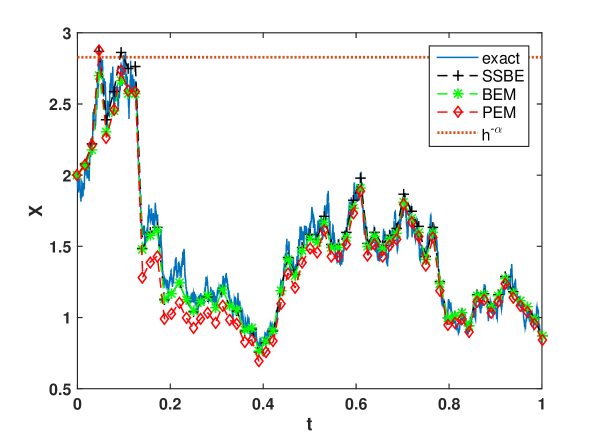
Figure 1. Single trajectories of each numerical method with step size $h=2^{-6}$ of the stochastic Ginzburg-Landau equation with parameters $\mu=0.5$, $\sigma=1$ and $X_{0}=2$. Threshold for the PEM projection is a shown as a dotted line.

In our experiments the SODE (41) is discretized by the split-step backward Euler method, the backward Euler-Maruyama scheme and the projected Euler-Maruyama method, respectively. Figure 1 shows single trajectories of the exact solution and the three numerical methods with equidistant step size $h=2^{-6}$ and parameter values $\mu=0.5$, $\sigma=1$, and $X_{0}=2$. Since Assumption 2.1 is satisfied with growth rate $q=3$, the parameter value $\alpha=\frac{1}{2(q-1)}=\frac{1}{4}$ is used for the PEM method. The implementation of the two implicit schemes SSBE and BEM employs Cardano’s method for directly solving the nonlinear equations. Further, for the simulation of the exact solution it is necessary to approximate the deterministic integral appearing in (42). This is done by a Riemann sum with step size $2^{-12}$.

Regarding the PEM method we are particularly interested in such trajectories which do not coincide with those generated by the standard Euler-Maruyama method. This event occurs when the scheme leaves the sphere of radius $h^{-\alpha}$ at least once and is then drawn back by the projection. More precisely, if it holds true that

(43) $$\big{\{}i=1,\ldots,N\;:\;|X_{h}^{\mathrm{PEM}}(t_{i})|>h^{-\alpha}\big{\}}\neq\emptyset,$$

then the PEM method deviates from the standard Euler-Maruyama scheme. In Figure 1 the trajectory of the PEM method crosses the line with height $h^{-\alpha}=2^{\frac{3}{2}}$ in the fourth step. Thereafter, the scheme seemingly underestimates the exact solution, although this effect vanishes when time evolves due to the dissipative nature of equation (41).

Obviously, this behavior is undesirable and the standard Euler-Maruyama method would have given a better approximation of the exact solution in this case. However, let us stress that the main purpose of the projection in the PEM method is to counteract the effect described by Hutzenthaler et al. [11], where the product of the norm of explosive trajectories by the explicit Euler-Maruyama method times the probability to observe such explosive trajectories goes to infinity as the step size goes to zero. Thus, the Euler-Maruyama values have no bounded moments in the limit $h\to 0$ and, consequently, it is divergent in the mean square sense.

On the other hand, the projection in the PEM method essentially prevents the numerical methods from leaving the ball with radius $h^{-\alpha}$. Due to the existence of higher moments, this also holds true for the exact solution up to a set of very small probability (c.f. with the proof of Lemma 6.5). Hence, while being possibly large, the error in such an instance remains essentially bounded and the line of arguments in [11] leading to the divergence of the standard Euler-Maruyama method does not apply to the PEM method.

Figure 2. Strong convergence errors for the approximation of the stochastic Ginzburg-Landau equation (41) with parameters $\mu=0.5$, $\sigma=1$, and $X_{0}=2$ for .

Table 1. Estimated errors and EOCs for the approximations of (41)

	SSBE		BEM		PEM
$h$	error	EOC	error	EOC	error	EOC	#-Proj.
$2^{-6}$	0.04637		0.04106		0.04553		33906
$2^{-7}$	0.03013	0.62	0.02808	0.55	0.02945	0.63	2157
$2^{-8}$	0.02029	0.57	0.01951	0.53	0.02002	0.56	26
$2^{-9}$	0.01396	0.54	0.01365	0.52	0.01384	0.53	0
$2^{-10}$	0.00975	0.52	0.00960	0.51	0.00968	0.52	0
$2^{-11}$	0.00683	0.51	0.00678	0.50	0.00681	0.51	0

Table 1 and Figure 2 show the estimated strong error of convergence for six different equidistant step sizes $h=2^{k-12}$, $k=1,\dots,6$. For simplicity we only estimate the error at the final time $T=1$, that is

(44) $$\text{error}=({\mathbb{E}}(|X_{h}(T)-X(T)|^{2}))^{\frac{1}{2}},$$

where $X_{h}(T)$ denotes the respective numerical approximations of the exact solution $X(T)$. The expected value is estimated by a Monte Carlo simulation based on $10^{6}$ sample paths. Our experiments indicate that the Monte Carlo error then drops well below the strong error to be estimated. As before the parameter values are $\mu=0.5$, $\sigma=1$, and $X_{0}=2$.

In Figure 2 one clearly observes strong order $\gamma=\frac{1}{2}$ for all three methods. Further, no numerical method has a significant advantage over one of the others. Table 1 also contains the estimates of the errors and the corresponding experimental order of convergence defined by

$$\text{EOC}=\frac{\log(\text{error}(h_{i}))-\log(\text{error}(h_{i-1}))}{\log(h_{i})-\log(h_{i-1})},\ i=2,\dots,k.$$

For each method we also computed an average of the experimental order of convergence by determining the best fitting line in a least-squares sense for the logarithmically scaled errors. The slopes of these lines are $0.55$, $0.52$, and $0.54$ for the SSBE, BEM, and PEM method, respectively.

Finally, the last column in Table 1 contains the number of Monte Carlo samples for which the trajectory of the PEM method leaves the sphere of radius $h^{-\alpha}$, that is the event described in (43) has occurred. Relating this to the total number of Monte Carlo samples we see that approximately $3.3$ percent of the PEM trajectories with step size $h=2^{-6}$ do not coincide with the trajectories of the standard Euler-Maruyama method. However, as the step size gets smaller the number of those samples drops quickly.

Note that we do not know if those excursions from the sphere of radius $h^{-\alpha}$ are caused by the explosive behavior of the standard Euler-Maruyama method described in [11] or if it is due to an intrinsic feature of the exact solution. In the latter case the projection may cause more harm than good. But in both cases a good advice is to choose a smaller step size if the relative frequency to observe the event (43) is too high.

This becomes even more evident in our next example, which consists of the following nonlinear SODE

(45) $$\begin{split}\,\mathrm{d}X(t)&=\lambda X(t)(\mu-|X(t)|)\,\mathrm{d}t+\sigma|X(t)|^{\frac{3}{2}}\,\mathrm{d}W(t),\\ X(0)&=X_{0},\end{split}$$

where $\lambda$, $\mu$, $\sigma$, $X_{0}\geq 0$. This equation incorporates a super-linearly growing diffusion coefficient function and is used as a stochastic volatility model (SVM) in mathematical finance [3]. It has also been considered in [21] for a tamed Euler method.

The mappings $f,\ g\colon{\mathbb{R}}\rightarrow{\mathbb{R}}$ defined by $f(x):=\lambda x(\mu-|x|)$ and $g(x):=\sigma|x|^{\frac{3}{2}}$ are continuous for all $x\in{\mathbb{R}}$ and satisfy the global monotonicity condition in Assumption 2.1 with $\eta\leq\frac{\lambda+\sigma^{2}}{\sigma^{2}}$ and $L=\lambda\mu$. Moreover, the coercivity condition (8) is fulfilled for every $p\leq\frac{2\lambda+\sigma^{2}}{\sigma^{2}}$. We refer to the Appendix in [21] for calculations of the constants $\eta$, $p$, and $L$.

For the numerical experiments the parameter values are $\lambda=3.5$, $\mu=3$, $\sigma=1$, and the initial value is $X_{0}=5$. Hence, the global monotonicity condition (3) is satisfied with $1<\eta<4.5$. Further, the exact solution fulfills $\sup_{t\in[0,T]}\|X(t)\|_{L^{p}(\Omega;{\mathbb{R}}^{d})}<\infty$ for every $p\leq 8$.

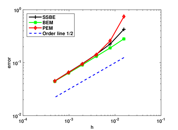
Figure 3. Strong convergence errors for the approximation of the $3/2$-volatility model (45) with parameters $\lambda=3.5,\mu=3,\sigma=1$ and $X_{0}=5$.

Table 2. Estimated errors and EOCs for the approximation of (45)

	SSBE		BEM		PEM
$h$	error	EOC	error	EOC	error	EOC	#-Proj.
$2^{-6}$	0.42856		0.28267		0.74770		139890
$2^{-7}$	0.22499	0.93	0.18973	0.58	0.25858	1.53	22338
$2^{-8}$	0.14359	0.65	0.13167	0.53	0.14208	0.86	2707
$2^{-9}$	0.09603	0.58	0.09119	0.53	0.09484	0.58	294
$2^{-10}$	0.06585	0.54	0.06371	0.52	0.06516	0.54	24
$2^{-11}$	0.04524	0.54	0.04454	0.52	0.04508	0.53	0

Since there is no explicit expression available, we replace the exact solution in (44) by a numerical reference approximation with a very fine step size $h_{\mathrm{ref}}=2^{-16}$. The implicit schemes are again implemented by solving the nonlinear equation in each time step explicitly. This time we take the parameter value $\alpha=\frac{1}{2}$ for the PEM method. As above our estimate of the errors are based on a Monte Carlo simulation with $10^{6}$ sample paths.

Figure 3 shows the strong convergence errors of the three methods with six different step sizes $h=2^{k}\Delta t$, $k=5,\dots,10$. The results are well in line with the predicted strong order $\gamma=\frac{1}{2}$ for all schemes provided that the step size is sufficiently small. In that case, there is again no significant difference in the behavior of the three schemes. For larger step sizes, however, the BEM methods outperforms the SSBE scheme and, on a much larger scale, the PEM method significantly.

This can also been seen from Table 2, which contains the numerical values for the strong errors shown in Figure 3. The values for the corresponding experimental order of convergence verify the theoretical results only for small values of $h$. As above we also determine an average experimental order of convergence for the three methods as the slope of the best fitting line in the mean-square sense. The results for the SSBE, BEM, and PEM method are $0.63$, $0.53$, and $0.77$, respectively.

Note that in the stochastic volatility method the magnitude of the noise term is, intentionally, much larger than in the Ginzburg-Landau equation while the damping in the drift term is weaker if $X(t)>\mu$. Thus, the dynamic is more often dominated by the noise term. It appears that the BEM scheme works best in this situation as the noise term is always damped by the implicit step. In the SSBE scheme, on the other hand, the most recent noise increment is undamped which apparently affects the error negatively if the step size is large. This effect is even worse for the explicit PEM scheme. In addition, the high noise intensity makes it more likely for the exact solution to leave the sphere of radius $h^{-\alpha}$ while the PEM method cannot follow and is pulled back. This coincides with a larger number of trajectories in which the projection has been applied as can be seen from the values in the last column of Table 2.

To conclude this section, let us summarize our observations: We have seen in the numerical experiments that the three schemes perform equally well if the step size is small enough. For larger step sizes the implicit schemes turned out to be superior over the PEM method, especially if the noise term is more likely to dominate the underlying dynamics. However, by observing the relative frequency of the event (43) one may have a simple indicator available if the step size of the explicit method should be further decreased. Since the PEM method is, in general, cheaper to simulate than the implicit schemes, one might afford this, eventually.

Acknowledgement

The authors wish to thank R. D. Grigorieff for calling our attention to the reference [22] and thereby pointing us to the concept of C-stability. Further, the first two authors gratefully acknowledge financial support by the DFG-funded CRC 701 ’Spectral Structures and Topological Methods in Mathematics’. The same holds true for the third named author, who has been supported by the research center Matheon. He also likes to thank the CRC 701 for making possible a very fruitful research stay at Bielefeld University, during which essential parts of this work were written. Finally, the authors wish to thank an anonymous referee and the associated editor for very helpful suggestions and comments.

References

[1]
A. Andersson and R. Kruse.
Mean-square convergence of the BDF2-Maruyama and backward Euler
schemes for SDE satisfying a global monotonicity condition.
Preprint, arXiv:1509.00609, 2015.
[2]
K. Dekker and J. Verwer.
Stability of Runge-Kutta methods for stiff nonlinear
differential equations, volume 2 of CWI monographs.
North-Holland, Amsterdam, 1984.
[3]
J. Goard and M. Mazur.
Stochastic volatility models and the pricing of VIX options.
Math. Finance, 23(3):439–458, 2013.
[4]
V. Grimm and G. R. W. Quispel.
Geometric integration methods that preserve Lyapunov functions.
BIT, 45(4):709–723, 2005.
[5]
E. Hairer and G. Wanner.
Solving ordinary differential equations. II, volume 14 of
Springer Series in Computational Mathematics.
Springer-Verlag, Berlin, second edition, 1996.
Stiff and differential-algebraic problems.
[6]
P. Henry-Labordère.
Solvable local and stochastic volatility models: supersymmetric
methods in option pricing.
Quant. Finance, 7(5):525–535, 2007.
[7]
D. J. Higham, X. Mao, and A. M. Stuart.
Strong convergence of Euler-type methods for nonlinear stochastic
differential equations.
SIAM J. Numer. Anal., 40(3):1041–1063, 2002.
[8]
Y. Hu.
Semi-implicit Euler-Maruyama scheme for stiff stochastic equations.
In H. Koerezlioglu, editor, Stochastic Analysis and Related
Topics V: The Silvri Workshop, volume 38 of Progr. Probab., pages
183–202, Boston, 1996. Birkhauser.
[9]
M. Hutzenthaler and A. Jentzen.
On a perturbation theory and on strong convergence rates for
stochastic ordinary and partial differential equations with non-globally
monotone coefficients.
Preprint, arXiv:1401.0295v1, 2014.
[10]
M. Hutzenthaler and A. Jentzen.
Numerical approximations of stochastic differential equations with
non-globally Lipschitz continuous coefficients.
Mem. Amer. Math. Soc., 236(1112):99, 2015.
[11]
M. Hutzenthaler, A. Jentzen, and P. E. Kloeden.
Strong and weak divergence in finite time of Euler’s method for
stochastic differential equations with non-globally Lipschitz continuous
coefficients.
Proc. R. Soc. Lond. Ser. A Math. Phys. Eng. Sci.,
467(2130):1563–1576, 2011.
[12]
M. Hutzenthaler, A. Jentzen, and P. E. Kloeden.
Strong convergence of an explicit numerical method for SDEs with
nonglobally Lipschitz continuous coefficients.
Ann. Appl. Probab., 22(4):1611–1641, 2012.
[13]
P. E. Kloeden and E. Platen.
Numerical Solution of Stochastic Differential Equations.
Springer, Berlin, third edition, 1999.
[14]
N. V. Krylov.
On Kolmogorov’s equation for finite dimensional diffusions.
In Stochastic PDE’s and Kolmogorov equations in infinite
dimensions (Cetraro, 1998), pages 1–63. Lecture Notes in Math., vol. 1715,
Springer, Berlin, 1999.
[15]
X. Mao.
Stochastic differential equations and their applications.
Horwood Publishing Series in Mathematics & Applications. Horwood
Publishing Limited, Chichester, 1997.
[16]
X. Mao and L. Szpruch.
Strong convergence rates for backward Euler-Maruyama method for
non-linear dissipative-type stochastic differential equations with
super-linear diffusion coefficients.
Stochastics, 85(1):144–171, 2013.
[17]
G. N. Milstein.
Numerical integration of stochastic differential equations,
volume 313 of Mathematics and its Applications.
Kluwer Academic Publishers Group, Dordrecht, 1995.
Translated and revised from the 1988 Russian original.
[18]
G. N. Milstein and M. V. Tretyakov.
Stochastic Numerics for Mathematical Physics.
Scientific Computation. Springer-Verlag, Berlin, 2004.
[19]
J. M. Ortega and W. C. Rheinboldt.
Iterative solution of nonlinear equations in several variables,
volume 30 of Classics in Applied Mathematics.
Society for Industrial and Applied Mathematics (SIAM), Philadelphia,
PA, 2000.
Reprint of the 1970 original.
[20]
C. Prévôt and M. Röckner.
A Concise Course on Stochastic Partial Differential Equations,
volume 1905 of Lecture Notes in Mathematics.
Springer, Berlin, 2007.
[21]
S. Sabanis.
Euler approximations with varying coefficients: the case of
superlinearly growing diffusion coefficients.
Preprint, arXiv:1308.1796v2, 2014.
[22]
K. Strehmel, R. Weiner, and H. Podhaisky.
Numerik gewöhnlicher Differentialgleichungen : nichtsteife,
steife und differential-algebraische Gleichungen.
Studium. Springer Spektrum, Wiesbaden, 2., rev. and ext. edition,
2012.
[23]
A. M. Stuart and A. R. Humphries.
Dynamical Systems and Numerical Analysis, volume 2 of Cambridge Monographs on Applied and Computational Mathematics.
Cambridge University Press, Cambridge, 1996.
[24]
L. Szpruch and X. Zhang.
-integrability, asymptotic stability and comparison theorem of
explicit numerical schemes for SDEs.
Preprint, arXiv:1310.0785v2, 2015.
[25]
M. V. Tretyakov and Z. Zhang.
A fundamental mean-square convergence theorem for SDEs with locally
Lipschitz coefficients and its applications.
SIAM J. Numer. Anal., 51(6):3135–3162, 2013.
[26]
X. Wang and S. Gan.
B-convergence of split-step one-leg theta methods for stochastic
differential equations.
J. Appl. Math. Comput., 38(1-2):489–503, 2012.