Electronic Structure Calculations with LDA+DMFT

Abstract

The LDA+DMFT method is a very powerful tool for gaining insight into the physics of strongly correlated materials. It combines traditional ab-initio density-functional techniques with the dynamical mean-field theory. The core aspects of the method are (i) building material-specific Hubbard-like many-body models and (ii) solving them in the dynamical mean-field approximation. Step (i) requires the construction of a localized one-electron basis, typically a set of Wannier functions. It also involves a number of approximations, such as the choice of the degrees of freedom for which many-body effects are explicitly taken into account, the scheme to account for screening effects, or the form of the double-counting correction. Step (ii) requires the dynamical mean-field solution of multi-orbital generalized Hubbard models. Here central is the quantum-impurity solver, which is also the computationally most demanding part of the full LDA+DMFT approach. In this chapter I will introduce the core aspects of the LDA+DMFT method and present a prototypical application.

1 The Strong Correlation Problem

In the non-relativistic limit electrons in a crystal are typically described by the Hamiltonian (in atomic units)

$$H = -\frac{1}{2}\sum_{i}\nabla^{2}_{i}+\frac{1}{2}\sum_{i\neq{i^{\prime}}}\frac{1}{|{\bf r}_{i}-{\bf r}_{i^{\prime}}|}-\sum_{i\alpha}\frac{Z_{\alpha}}{|{\bf r}_{i}-{\bf R}_{\alpha}|}+\frac{1}{2}\sum_{\alpha\neq\alpha^{\prime}}\frac{Z_{\alpha}Z_{\alpha^{\prime}}}{|{\bf R}_{\alpha}-{\bf R}_{\alpha^{\prime}}|}$$ (1)

$$= {T}_{e}+{V}_{ee}+{V}_{en}+{V}_{nn},$$

where $\{{\bf r}_{i}\}$ are the coordinates of the $N_{e}$ electrons, $\{{\bf R}_{\alpha}\}$ those of the $N_{n}$ nuclei, $Z_{\alpha}$ their atomic numbers, and $M_{\alpha}$ their masses. Although it appears innocent, the Schrödinger equation $H_{e}\psi=\varepsilon\psi$ has a simple solution only in the non-interacting electron limit (${V}_{ee}=0$). In such a case it is sufficient to find the eigenvalues and eigenvectors of the one-electron Hamiltonian

$${h}({\bf r})=-\frac{1}{2}\nabla^{2}-\sum_{\alpha}\frac{Z_{\alpha}}{|{\bf r}-{\bf R}_{\alpha}|}=-\frac{1}{2}\nabla^{2}+v_{\rm ext}({\bf r}).$$

In a crystal, because of lattice translational invariance, the eigenvectors of ${h}_{e}({\bf r})$ are Bloch functions, $\psi_{n{\bf k}\sigma}({\bf r})$, and the eigenvalues band energies, $\varepsilon_{n{\bf k}}$; the many-body $N_{e}$-electron states can be then built from the Bloch states as Slater determinants. For an interacting system ($V_{ee}\neq 0$) we are, however, left in the realm of approximations.

In some limit the independent-particle picture still holds. Landau Fermi-liquid theory suggests that, at low enough energy and temperature, the elementary excitations of the interacting Hamiltonian (1) could be described by almost independent Fermionic quasi particles, Fermions with heavy masses $m^{*}$ and finite life-time $\tau^{\rm QP}$

$$\varepsilon_{n{\bf k}}^{\rm QP} = \frac{m}{m^{*}}\varepsilon_{n{\bf k}},$$

$$\tau^{\rm QP} \propto (aT^{2}+b\omega^{2})^{-1}.$$

Remarkably, a very large number of materials do exhibit low-energy Fermi-liquid behavior, and a violation of the Fermi-liquid picture is typically an indication that something surprising is going on.

Starting from a different perspective, using the standard model of solid state physics, the density-functional theory (DFT) lda ; barth ; martin , one can show that (1) can be mapped into an auxiliary one-electron problem (Kohn-Sham equations) where the external potential is replaced by

$$v_{\rm R}({\bf r})=-\sum_{\alpha}\frac{Z_{\alpha}}{|{\bf r}-{\bf R}_{\alpha}|}+\int d{\bf r}^{\prime}\frac{n({\bf r}^{\prime})}{|{\bf r}-{\bf r}^{\prime}|}+\frac{\delta E_{xc}[n]}{\delta n},$$

and $n({\bf r})$ is the electronic ground-state density. The first term of $v_{\rm R}({\bf r})$ is the external electron-nuclei interaction, the second is the long-range Hartree interaction and the third is the exchange-correlation potential. The DFT exchange-correlation functional $E_{xc}[n]$ is universal but also unknown. Thus, although DFT is in principle an exact ground-state theory, in practice we work with approximated forms of $E_{xc}[n]$. The most common approximation is the local-density approximation (LDA), in which $E_{xc}[n]$ is replaced by its expression for an interacting homogeneous electron gas,

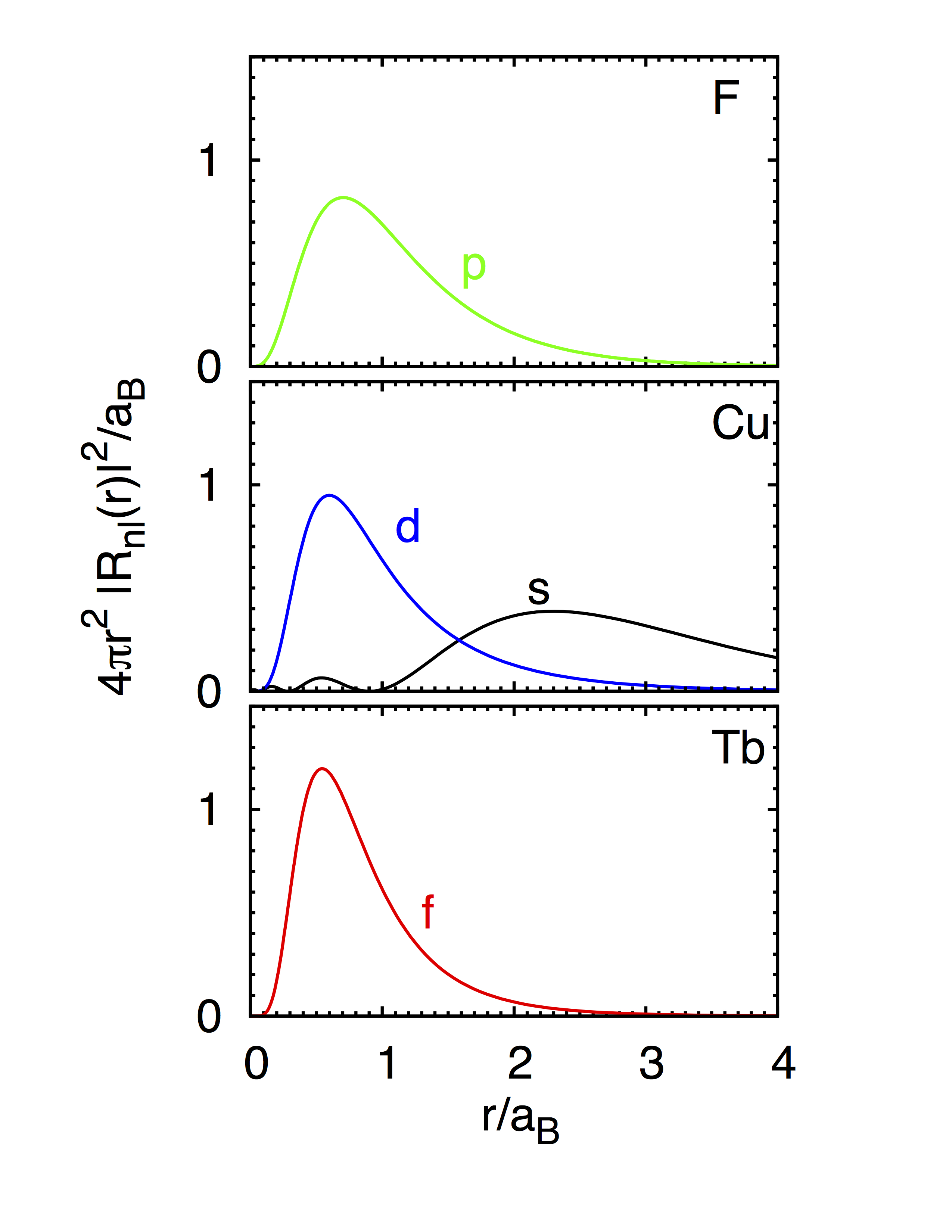
Figure 1: Localization of atomic orbitals (calculated in the LDA approximation) in exemplary cases: F ($p$), Cu ($d$ and $s$), and Tb ($f$) atoms. The figure shows $4\pi r^{2}|R_{nl}(r)|^{2}/a_{B}$ as a function of the distance from the position of the nucleus, $r/a_{B}$.

$$E_{xc}[n]\sim\int d{\bf r}\;\epsilon_{xc}^{\rm LDA}(n({\bf r}))n({\bf r}).$$ (2)

The LDA appears particularly justified if $n({\bf r})$ varies slowly in space. In this limit we can think of splitting space into regions in which the density is basically constant and the system can indeed be described by an interacting homogeneous electron gas with a given ground-state electron density $n({\bf r})$. By adding up the contributions of all these regions we can obtain expression (2).

The LDA and its generalizations have opened the path to ab-initio electronic-structure calculations, leading to the astonishing successes of DFT in explaining and predicting the electronic properties of complex materials lda . Even if Kohn-Sham eigenergies and orbitals are mathematically only the solution of an auxiliary problem, they proved very useful to describe the electronic structure of materials, even at finite temperature and for excited states.

This is not, however, the full story. For some systems simple approximations to the exchange-correlation functional such as the LDA qualitatively fail. These are the so-called strongly correlated systems, materials in which many-body effects manifest themselves in the form of emergent co-operative phenomena. A paradigmatic example is that of Mott insulators. Because of Coulomb repulsion, several transition-metal compounds with partially filled $d$ shells are experimentally paramagnetic insulators in a large temperature range, despite being described as good metals in LDA. Simple improvements of the LDA functional do not solve the discrepancy. Other examples are high-temperature superconducting cuprates, heavy Fermions, Kondo systems, and correlated organic crystals. The problem is usually the description of many-body effects between localized electrons from open $d$ or $f$ shells (see Figure 1). Because of the strong Coulomb repulsion, the dynamics of a single electron depends on the position of all other electrons, and cannot be understood within an independent electron picture, as the one arising from simple approximations to the DFT exchange-correlation functional.

It is interesting to observe that for several strongly correlated systems the Fermi-liquid picture still holds in the low-energy regime, although the effective masses can reach extreme values, as in heavy Fermions. One could therefore think of finding some effective potential that yields such very high masses. The actual energy region of validity of the Fermi-liquid theory for a given system is however unknown and it might be very narrow. This is typically the case for heavy-Fermions. Furthermore Fermi-liquid theory relies on perturbation theory, and inherently non-perturbative many-body phenomena are known. In systems such as Mott insulators even the Fermi-liquid picture breaks down.

In the lack of a better option, the study of strong correlations effects has been confined for a long time to simple many-body models. This minimal approach lead to striking successes, such as understanding the mechanism of the Kondo effect in diluted magnetic alloys, or to important developments in many-body theory, among which also the dynamical mean-field theory (DMFT) can be counted dmft ; rmp . Nevertheless, simple models are hardly sufficient to describe the complications of many-body effects in real materials. Thus during the years various attempts had been made to combine ab-initio techniques and many-body methods Hewson . The breakthrough came with the development of the LDA+DMFT (local-density approximation + dynamical mean-field theory) method original .

The LDA+DMFT approach can be roughly split into two steps. The first consists in building optimal material-specific many-body models, exploiting the power of practical DFT. In this step we construct a localized single-electron basis and calculate the parameters of the many-body model in such a basis. Crucial in model building is the identification of the electrons responsible for correlation effects. The second step consists in solving the resulting generalized Hubbard-like model with DMFT or, if possible, its extensions. Here one is faced with other challenges, in particular the solution of the DMFT quantum-impurity problem. Typically this is the computationally most demanding part of the approach. In this introductory chapter I discuss the two main steps of the LDA+DMFT method, and I present a characteristic application. A more extended introduction can be found in Ref. eva2011 ; more details on model building or quantum impurity solvers are given in Refs. book2011 ; book2012 . Other reviews on the LDA+DMFT method an its successes are Refs. georges ; georges2 ; imada ; kotliar .

2 Material-Specific Many-Body Models from DFT

The successes of the LDA suggest that the LDA Kohn-Sham orbitals carry the essential information about the structure and bonding of a given material. Thus they are best suited as a starting point to construct bases for material-specific many-body models. In recent years it has been shown that indeed a successful scheme consists in building localized Wannier functions $\psi_{in\sigma}({\bf r})$ from LDA Bloch functions

$$\psi_{in\sigma}({\bf r})=\frac{1}{\sqrt{N}}\sum_{{\bf k}}e^{-i{\bf R}_{i}\cdot{\bf k}}\;\psi_{n{\bf k}\sigma}({\bf r}).$$

Localized Wannier functions can be obtained in different ways. Successful methods are the ab-initio downfolding procedure based on the NMTO approach njp ; olebook2012 , the maximally-localized Wannier functions algorithm of Marzari and Vanderbilt mlwf and projector techniques projectors . In the LDA Wannier basis the many-body Hamiltonian (1) takes the form

$${H}={H}_{\rm LDA}+H_{U}-{H}_{\rm DC}.$$ (3)

The first term, $H_{\rm LDA}$, corresponds to the sum of the kinetic and potential energy ($T_{e}+V_{en}$), and can be expressed as

$${H}_{\rm LDA}=-\sum_{\sigma}\sum_{ii^{\prime}}\sum_{mm^{\prime}}t^{i,i^{\prime}}_{m,m^{\prime}}c^{\dagger}_{im\sigma}c^{\phantom{\dagger}}_{i^{\prime}m^{\prime}\sigma},$$

where $c^{\dagger}_{im\sigma}$ ($c^{\phantom{\dagger}}_{im\sigma}$) creates (destroys) an electron with spin $\sigma$ in orbital $m$ at site $i$, and the elements of matrix are

$$t^{i,i^{\prime}}_{m,m^{\prime}}=-\int d{\bf r}\,\overline{\psi}_{im\sigma}({\bf r})\left[-\frac{1}{2}\nabla^{2}+v_{\rm R}({\bf r})\right]\psi_{i^{\prime}m^{\prime}\sigma}({\bf r}).$$

The on-site ($i=i^{\prime}$) matrix is the crystal-field and the $i\neq i^{\prime}$ contributions are the hopping integrals. The Coulomb interaction $H_{U}$ is given by

$$H_{U}=\frac{1}{2}\sum_{ii^{\prime}jj^{\prime}}\sum_{\sigma\sigma^{\prime}}\sum_{mm^{\prime}}\sum_{pp^{\prime}}U_{mp\;m^{\prime}p^{\prime}}^{iji^{\prime}j^{\prime}}c^{\dagger}_{im\sigma}c^{\dagger}_{jp\sigma^{\prime}}c^{\phantom{\dagger}}_{j^{\prime}p^{\prime}\sigma^{\prime}}c^{\phantom{\dagger}}_{i^{\prime}m^{\prime}\sigma}.$$

The bare Coulomb integrals are

$$U_{np\;n^{\prime}p^{\prime}}^{iji^{\prime}j^{\prime}} = \!\int\!d{\bf r}_{1}\!\!\int\!d{\bf r}_{2}\;\overline{\psi}_{in\sigma}({\bf r}_{1})\overline{\psi}_{jp\sigma^{\prime}}({\bf r}_{2})\frac{1}{|{\bf r}_{1}-{\bf r}_{2}|}\psi_{j^{\prime}p^{\prime}\sigma^{\prime}}({\bf r}_{2})\psi_{i^{\prime}n^{\prime}\sigma}({\bf r}_{1}).$$ (4)

The term ${H}_{\rm DC}$ (double-counting correction) cancels the electron-electron interaction contained in ${H}^{\rm LDA}$ but also explicitly described by $H_{U}$. Although such term is in principle unknown, reasonable approximations have been developed in the context of the LDA+$U$ approach ldau , a method which shares the model building part with LDA+DMFT, and are successfully used also in LDA+DMFT calculations book2011 ; book2012 .

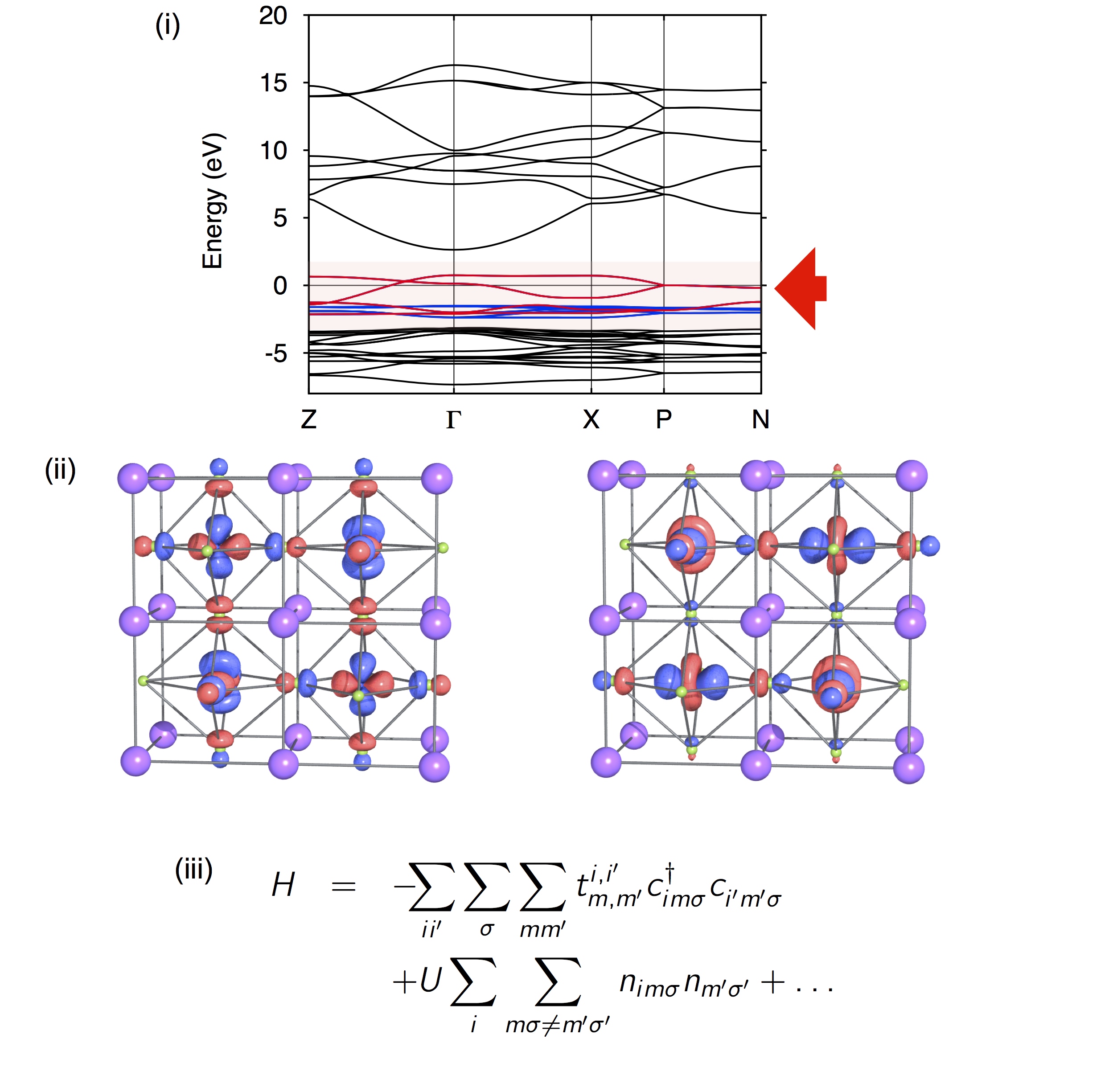
Figure 2: Building minimal material-specific many-body models in steps: (i) Full LDA band structure of the perovskite KCuF₃: The region with a red background shows the low-energy states, the Cu $d$ bands. They split into partially filled $e_{g}$ (red) and occupied $t_{2g}$ (blue). The $e_{g}$ bands are identified as the correlated states. (ii) Massive downfolding: Crystal-field Wannier functions basis spanning the $e_{g}$ bands in order (left to right) of decreasing crystal-field energy. The Wannier functions are plotted at each Cu site to show the site symmetries. (iii) Low-energy generalized Hubbard model for the $e_{g}$ bands.

The Hamiltonian (3) still describes the full many-body problem, whose solution remains inaccessible. It is therefore necessary to devise approximations to reduce the complexity of the problem to the essential. The most important one consists in separating the electrons in two types, the correlated or heavy electrons, for which LDA fails, and the uncorrelated or light electrons, for which LDA works sufficiently well (Fig. 2). The correction to LDA, $H_{U}-{H}_{\rm DC}$, is then taken into account explicitly only for the correlated electrons, typically chosen as those stemming from partially filled localized $d$ and $f$ atomic shells (Fig. 1). By truncating $H_{U}-{H}_{\rm DC}$ to the heavy-electron sector we implicitly assume that the main effect of light electrons is the effective screening of the Coulomb parameters for heavy electrons. Thus the bare Coulomb integrals (4) are replaced by screened parameters. The calculation of effective screened Coulomb couplings remains a major challenge to date. Approximate schemes developed so far are the constrained LDA (cLDA) approach cLDA and the constrained RPA (cRPA) method cRPA . In the first the screened $U$ is computed from the second derivative of the total energy as a function of the density; the hopping integrals between heavy and light electrons are cut to avoid electron transfer between light and heavy electrons sectors. In cRPA the polarization (and thus the screened Coulomb interaction) is obtained in the random-phase approximation by downfolding the uncorrelated sector, assuming that the latter is well described by mean field theory. The last important approximation is the assumption that the Coulomb interaction is local or very fast decaying. The successes of practical DFT suggest that the long-range Hartree and the mean-field exchange-correlation interaction are well described by the LDA or its extensions; we then can expect that the $H_{U}-{H}_{\rm DC}$ term is all the rest, i.e., that it is local (on-site) or almost local (between first nearest neighbors).

By means of these simplifications we have transformed the full many-body problem (1) to a minimal material-specific generalized Hubbard model with local or almost local Coulomb interaction. Even such a model cannot be solved exactly; as we will see in the next section, the dynamical mean-field approximation allows us, however, to capture the microscopic mechanisms behind emergent phenomena such as the Mott transition or orbital order.

In the rest of this paragraph we discuss in some more detail the form of the local Coulomb term. Correlated electrons partially retain their atomic character. Thus they are usually identified through the quantum numbers $lm\sigma$ of the atomic shells from which they stems. If $H_{U}-{H}_{\rm DC}$ is local and correlated electrons belong to a given shell (e.g., $d$ electrons, $l=2$), the screened Coulomb interaction can be written as $H_{U}-{H}_{\rm DC}\sim H_{U}^{l}-H_{\rm DC}^{l}$, with

$$H_{U}^{l}-H_{\rm DC}^{l}=\frac{1}{2}\sum_{i}\sum_{\sigma\sigma^{\prime}}\sum_{mm^{\prime}}\sum_{\tilde{m}\tilde{m}^{\prime}}U^{l}_{m\tilde{m}m^{\prime}\tilde{m}^{\prime}}c^{\dagger}_{im_{\sigma}}c^{\dagger}_{i\tilde{m}\sigma^{\prime}}c^{\phantom{\dagger}}_{i\tilde{m}^{\prime}\sigma^{\prime}}c^{\phantom{\dagger}}_{im^{\prime}\sigma}-H_{\rm DC}^{l}$$

where $m,m^{\prime},\tilde{m},\tilde{m}$ run from $-l$ to $l$, and ${H}_{\rm DC}^{l}$ is the mean-field (e.g., Hartree or Hartree-Fock) value of $H_{U}^{l}$. The screened Coulomb interaction has the same form of the bare interaction but it has renormalized $U^{l}_{m\tilde{m}m^{\prime}\tilde{m}^{\prime}}$ parameters. For simplicity we discuss it in the basis of atomic orbitals, $\psi_{nlm}({\bf r})=R_{nl}(r)Y_{m}^{l}(\theta,\phi)$. Thus

$$U_{mmm^{\prime}\tilde{m}^{\prime}}^{l}=\sum_{k=0}^{2l}a_{k}^{l}(mm^{\prime},\tilde{m}\tilde{m}^{\prime})F_{k}^{l},$$

where the angular integrals are

$$a_{k}^{l}(mm^{\prime},\tilde{m}\tilde{m}^{\prime})=\frac{4\pi}{2k+1}\sum_{q=-k}^{k}\langle lm|Y_{q}^{k}|lm^{\prime}\rangle\langle l\tilde{m}|\overline{Y}_{q}^{k}\>|l\tilde{m}^{\prime}\rangle,$$

and the radial Slater integrals are

$$F_{k}^{l}=\int\!d{r}_{1}\>r_{1}^{2}\int\!d{r}_{2}\>r_{2}^{2}\>R^{2}_{nl}(r_{1})\frac{r_{<}^{k}}{r_{>}^{k+1}}R_{nl}^{2}(r_{2}).$$

The most important Coulomb integrals are the direct ($U_{mm^{\prime}mm^{\prime}}^{l}$) and exchange ($U_{mm^{\prime}m^{\prime}m}^{l}$, with $m\neq m^{\prime}$) integrals, which can be expressed as

$$U_{mm^{\prime}mm^{\prime}}^{l}=U_{m,m^{\prime}} = \sum_{k=0}^{2l}a_{k}^{l}(mm,m^{\prime}m^{\prime})F_{k}^{l},$$

$$U_{mm^{\prime}m^{\prime}m}^{l}=J_{m,m^{\prime}} = \sum_{k=0}^{2l}a_{k}^{l}(mm^{\prime},m^{\prime}m)F_{k}^{l}.$$

The average Coulomb parameters are

$$U_{avg} = \frac{1}{(2l+1)^{2}}\sum_{m,m^{\prime}}U_{m,m^{\prime}}=F_{0}^{2},$$

$$U_{avg}-J_{avg} = \frac{1}{2l(2l+1)}\sum_{m,m^{\prime}}(U_{m,m^{\prime}}-J_{m,m^{\prime}}).$$

For atomic states $U_{\rm avg}$ is very large (typically $15-20$ eV for $d$ electrons) but is drastically reduced by screening effects. For $d$ shells ($l=2$) only $F_{0}^{2}$, $F_{2}^{2}$ and $F_{4}^{2}$ contribute to the Coulomb integrals, and $J_{\rm avg}=(F_{2}^{2}+F_{4}^{2})/14$. For hydrogen-like 3$d$ orbitals, $F_{4}^{2}/F_{2}^{2}=15/23$, while for realistic 3$d$ orbitals this ratio is slightly smaller; a typical value of the ratio $F_{4}^{2}/F_{2}^{2}$ is $\sim 0.625=5/8$.

It is useful to re-express the parameters $U_{m,m^{\prime}}$ and $J_{m,m^{\prime}}$ as a function of the following three parameters

$$U_{0} = U_{\rm avg}+\frac{8}{7}J_{\rm avg}=U_{\rm avg}+\frac{8}{5}{\cal{J}}_{\rm avg}$$

$${\cal{J}}_{avg} = \frac{1}{2l(2l+1)}\sum_{m\neq m^{\prime}}J_{m,m^{\prime}}=\frac{5}{7}J_{\rm avg}$$

$$\Delta{\cal{J}}_{avg} = {\cal{J}}_{avg}\left(\frac{1}{5}-\frac{1}{9}\frac{F_{4}^{2}}{F_{2}^{2}}\right)/\left(1+\frac{F_{4}^{2}}{F_{2}^{2}}\right)$$

Here $U_{0}$ is the orbital-diagonal direct Coulomb integral; ${\cal{J}}_{avg}$ the average interaction in the basis of cubic harmonics, typically used in electronic calculations; $\Delta{\cal{J}}_{avg}$ measures the orbital anisotropy of the Coulomb interaction. For the $d$ shell the matrix $U_{m,m^{\prime}}-U_{0}$ may then be written as (see Appendix)

$$\begin{array}[]{l|cccccc}U_{m,m^{\prime}}-U_{0}&|xy\rangle&|yz\rangle&|3z^{2}-r^{2}\rangle&|xz\rangle&|x^{2}-y^{2}\rangle\\[4.30554pt] \hline\cr\\ |xy\rangle&0&-2J_{1}&-2J_{2}&-2J_{1}&-2J_{3}\\ |yz\rangle&-2J_{1}&&-2J_{4}&-2J_{1}&-2J_{1}\\ |3z^{2}-r^{2}\rangle&-2J_{2}&-2J_{4}&0&-2J_{4}&-2J_{2}\\ |xz\rangle&-2J_{1}&-2J_{1}&-2J_{4}&0&-2J_{1}\\ |x^{2}-y^{2}\rangle&-2J_{3}&-2J_{1}&-2J_{2}&-2J_{1}&0\\[4.30554pt] \end{array}$$ (5)

where the exchange integrals $J_{m,m^{\prime}}$ appearing in (5) are

$$J_{1}={\cal{J}}_{\rm avg}+\Delta{\cal{J}}_{\rm avg},$$

$$J_{2}={\cal{J}}_{\rm avg}+3\Delta{\cal{J}}_{\rm avg},$$

$$J_{3}={\cal{J}}_{\rm avg}-5\Delta{\cal{J}}_{\rm avg},$$

$$J_{4}={\cal{J}}_{\rm avg}-3\Delta{\cal{J}}_{\rm avg}.$$

The Coulomb anisotropy $\Delta{\cal{J}}_{\rm avg}$ is crucial for a proper description of the multiplet structure, and is particular important for systems close to spin-state transitions, such as cobaltates ss . Various approximations of the Coulomb interaction are often adopted in LDA+DMFT calculations; they are typically introduced to reduce the complexity of the calculation and the CPU-time or to make the problem tractable in the first place. One has to keep in mind that these approximations alter the structure of the multiplets, and their validity has to be considered case by case. Perhaps the most common approximation of the Coulomb interaction is the density-density approximation, in which only Coulomb terms that can be expressed as density-density interaction are retained. This approximation is typically adopted when the Hirsch-Fye quantum Monte Carlo (HF-QMC) algorithm hirsch is used as DMFT quantum-impurity solver. To go beyond it with QMC has required the development of a new algorithm, the continuous-time QMC approach (CT-QMC) ctqmc .

3 The Dynamical Mean-Field Approximation

The separation of electrons in light and heavy greatly simplifies the problem, reducing the many-body Hamiltonian (1) to a generalized Hubbard model. Nevertheless, the exact solution of such a many-body problem remains out of reach. The DMFT dmft is to date the best approximate method which still retains the essential ingredients to explain strong correlation phenomena such as the Mott metal-insulator transition or orbital ordering.

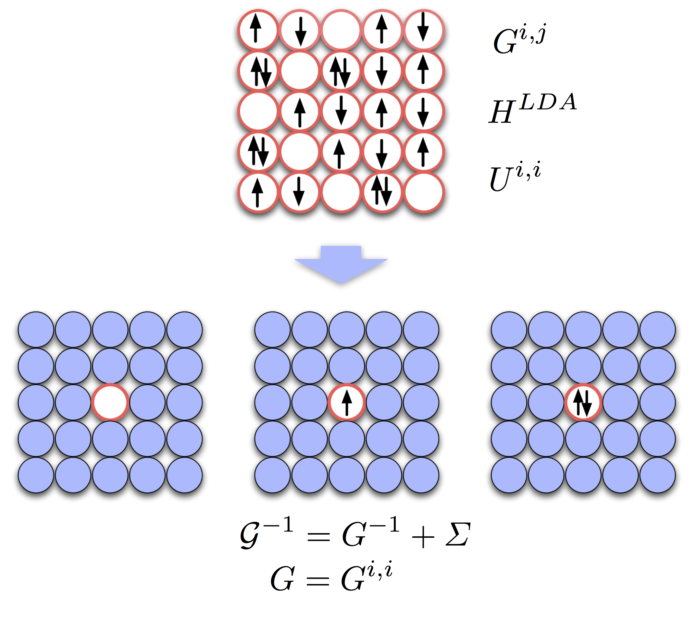
In DMFT the lattice many-body Hubbard model is mapped onto an effective single-impurity model which describes a single correlated site in an effective bath (Fig. 3). The exact solution of a such a quantum-impurity problem is hard, but this time various numerically exact techniques are available.

Figure 3: Schematic illustration of the dynamical mean-field approximation. The lattice Hubbard model is mapped onto an effective quantum-impurity problem satisfying the condition $G=G^{i,i}$, where $G^{i,i}$ is the local lattice Green-function matrix and $G$ the Green-function matrix of the impurity problem. The self-energy matrix is dynamical ($\omega$-dependent) but local (k-independent). The dynamical mean-field theory is exact in the limit of infinite coordination number dmft .

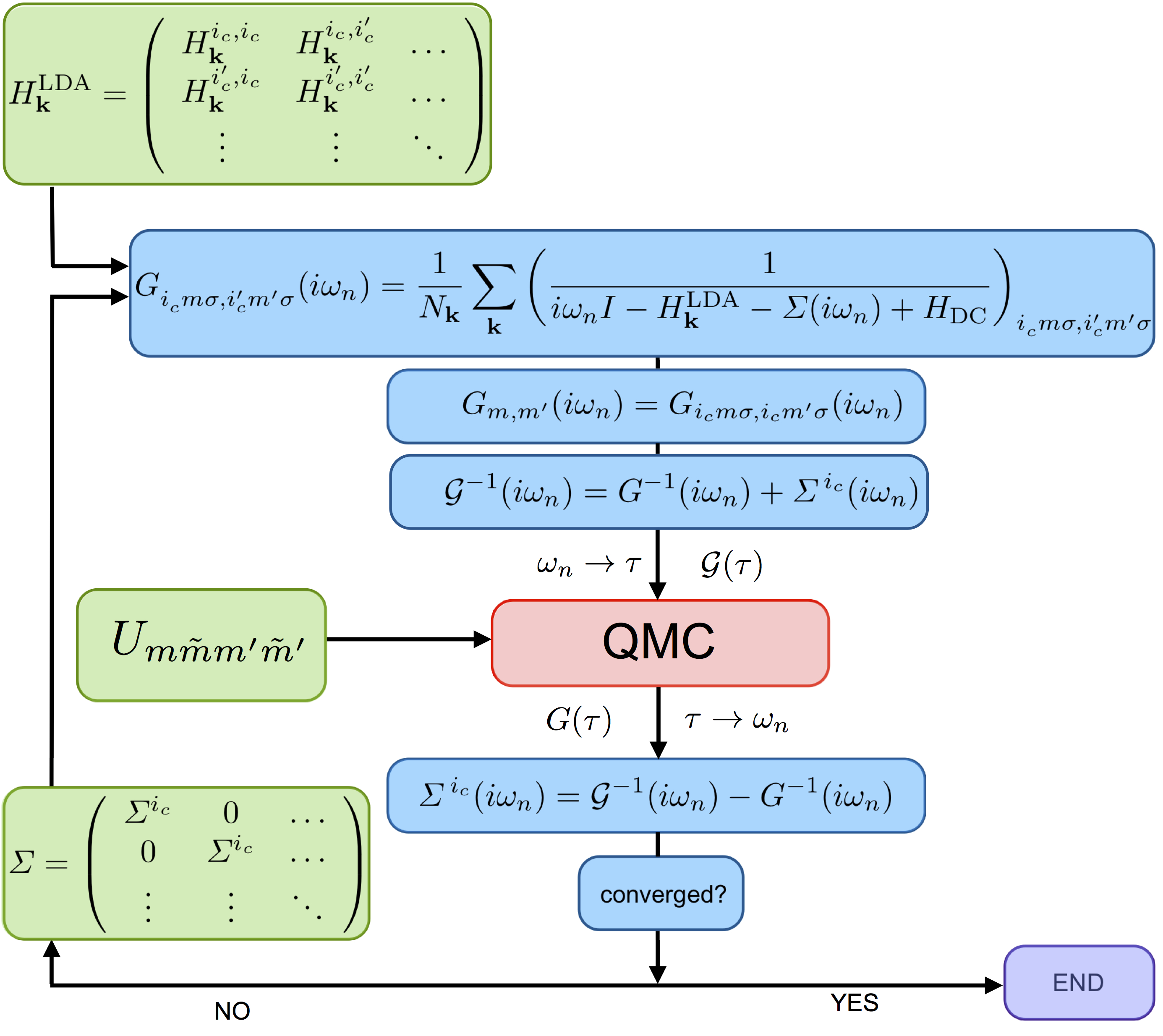
The various steps of LDA+DMFT are shown in Fig. 4. Let us assume we followed the procedure described in the previous section. In the example of the KCuF₃ perovskite of Fig. 2 we identify the $e_{g}$ states as correlated electrons. The minimal model for such a system is a 2-band $e_{g}$ Hubbard model, and the smallest possible unit cell has two equivalent correlated sites. More generally, we can assume that a system is described by a unit cell with $i_{c}=1,\dots,n_{c}$ equivalent correlated sites and at each correlated site we label the correlated orbitals with $\{m\sigma\}$; a number of non-correlated orbitals and sites are also in general included in the model.

To solve with DMFT the Hubbard-like model for our system we first map it onto a quantum-impurity problem. Next we solve the latter self-consistently, i.e., with the constraint that the impurity Green-function matrix $G(\omega)$ equals the local lattice Green-function matrix $G^{\>i_{c},i_{c}}(\omega),$

$$G_{m,m^{\prime}}(\omega)=G^{\>i_{c},i_{c}}_{m\sigma,m^{\prime}\sigma}(\omega).$$

To do this we use an iterative procedure. First we calculate the local lattice Green-function matrix for a given bath, i.e.,

Figure 4: LDA+DMFT self-consistency loop for a system with $\{m\}$ orbital degrees of freedom and at least two equivalent correlated sites. We assume that a quantum Monte Carlo impurity solver is used, and that the quantum-impurity problem is then solved in imaginary time $\tau$ and Matsubara frequencies $\omega_{n}$.

$$G^{\>i_{c},i_{c}}_{m\sigma,m^{\prime}\sigma}(\omega)=\frac{1}{N_{\bf k}}\sum_{\bf k}\left(\frac{1}{{(\omega+\mu)I-{H}_{\bf k}^{\rm LDA}-\Sigma(\omega)+{H}_{\rm DC}}}\right)_{i^{\phantom{{}^{\prime}}}_{c}m\sigma,i_{c}^{\prime}m^{\prime}\sigma},$$

where ${H}_{\bf k}^{\rm LDA}$ is the LDA Hamiltonian in k space, and $\Sigma(\omega)$ is the self-energy matrix; to first iteration we can assume that the bath Green-function matrix is the local LDA Green-function matrix and that the self-energy is therefore zero. In the next iterations, the DMFT self-energy matrix is non-zero in the correlated sector (sites $\{i_{c}\}$ and orbitals $\{m\}$). Furthermore it is local, i.e.,

$$\Sigma_{m\sigma,m^{\prime}\sigma}^{i_{c}^{\phantom{{}^{\prime}}},i_{c}^{\prime}}(\omega)=\delta_{i_{c}^{\phantom{{}^{\prime}}},i_{c}^{\prime}}\Sigma^{\,i_{c}\sigma}_{m,m^{\prime}}(\omega).$$

For two equivalent correlated sites $i_{c}^{\phantom{{}^{\prime}}}$ and $i_{c}^{\prime}$, space group symmetries transform $\Sigma^{\,i_{c}^{\phantom{{}^{\prime}}}\sigma}_{m,m^{\prime}}$ into $\Sigma^{\,i_{c}^{\prime}\sigma}_{m,m^{\prime}}$. For convenience we can instead use the same symmetries to transform the LDA Hamiltonian in such way that its on-site blocks are identical for equivalent correlated sites. Then

$$\Sigma^{\,i_{c}\sigma}_{m\sigma,m^{\prime}\sigma}(\omega)=\Sigma^{\sigma}_{m,m^{\prime}}(\omega).$$

In the paramagnetic phase an additional relation holds, i.e.

$$\Sigma^{\sigma}_{m,m^{\prime}}(\omega)=\Sigma^{-\sigma}_{m,m^{\prime}}=\Sigma_{m,m^{\prime}}(\omega).$$

The bath Green function of the single impurity model can be obtained from the Dyson equation

$$\quad{\cal{G}}^{-1}(\omega)=G^{-1}(\omega)+\Sigma(\omega).$$

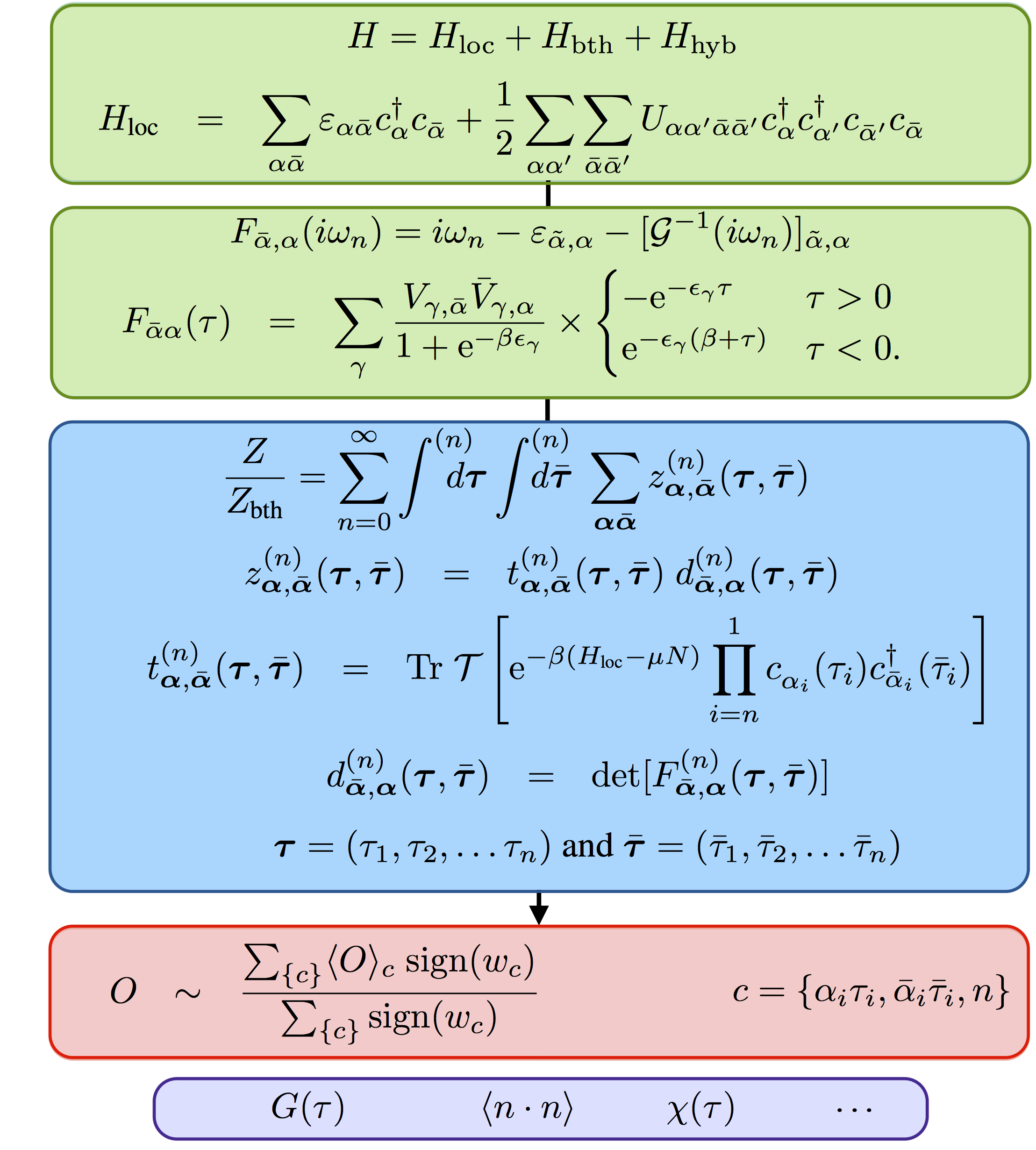
Figure 5: Schematic representation of the most important steps in CT-HYB QMC ctqmc , following the notation of Ref. ctqmcflesch . The impurity Hamiltonian is split into local ($H_{\rm loc}$), bath ($H_{\rm bth}$) and hybridization ($H_{\rm hyb}$) term. The bath Green function yields the hybridization function $F$, which together with the local Hamiltonian makes up the input to the QMC simulation. In the next step, the partition function is expanded in even orders $2n$ of $H_{\rm hyb}$ and bath degrees of freedom are integrated out. To obtain a given observable, configurations (made of expansion orders $n$, flavors ${\alpha_{i}}=m_{i}\sigma_{i}$, and imaginary times ${\bf\tau}_{i},\bar{\tau}_{i}$) are sampled via a Monte Carlo procedure. The bottleneck is the calculation of the local trace $t^{(n)}$ which requires multiplications of creator and annihilator matrices as well as the propagation of vectors in imaginary time. In the so-called Krylov scheme a number basis is used so that all operators are sparse matrices and the Lanczos algorithm is used in the propagation of vectors. A considerable reduction in computational time can be achieved by exploiting symmetries.

The quantum-impurity problem, defined by the correlated impurity and the bath Green-function matrix, is then solved via a quantum-impurity solver, which yields a new impurity Green-function matrix, $G_{m,m^{\prime}}(\omega)$. A new self-energy is obtained from the Dyson equation

$$\quad\Sigma(\omega)={\cal{G}}^{-1}(\omega)-G^{-1}(\omega).$$

The procedure is repeated till self-consistency is reached.

The core of the DMFT simulation is the solution of the multi-orbital quantum-impurity model, i.e. finding $G(\omega)$ for a given $\cal{G}(\omega)$ and Coulomb interaction. Several numerically exact approaches exist, the most important being Quantum Monte Carlo hirsch ; ctqmc , Lanczos lanczos ; erik , the numerical renormalization group, and many more. Each technique is best suited to deal with certain types of problems. Perhaps to date the most flexible methods are those based on QMC techniques. The Hirsch-Fye QMC hirsch approach is very general. A limitation is that spin-flip and pair-hopping terms have to be neglected; in all cases in which the multiplet structure is not crucial, this is, however, a very good approximation. A second limitation of HF-QMC is that, for multi-orbital systems, low temperatures can only be reached at prohibitive cost. The continuous-time QMC technique ctqmc is based on the expansion of the partition function in powers of the hybridization (CT-HYB) or the interaction (CT-INT), and can treat spin-flip and pair-hopping terms; the CT-HYB algorithm is the one best suited to reach experimental temperatures for realistic models; CT-INT can deal more efficiently with clusters extensions of DMFT. A schematic representation of the CT-HYB technique is given in Fig. 5. A drawback of all QMC techniques discussed so far is that they yield results on the imaginary axis, and the analytic continuation requires techniques such as the maximum entropy method Jarrell or stochastic approaches Mit . Real-frequency methods such as exact diagonalization or Lanczos have the advantage that they give access directly to the real axis, and are fast; they require however large memory; furthermore, in these techniques the bath is discretized, and the convergence with the number of bath sites can be very slow, in particular in small-gap systems. Apart from numerically exact approaches, approximate solvers are also often adopted: various Hubbard approximations, the iterative perturbation theory, the one-crossing approximation, the Gutzwiller variational approach, or others.

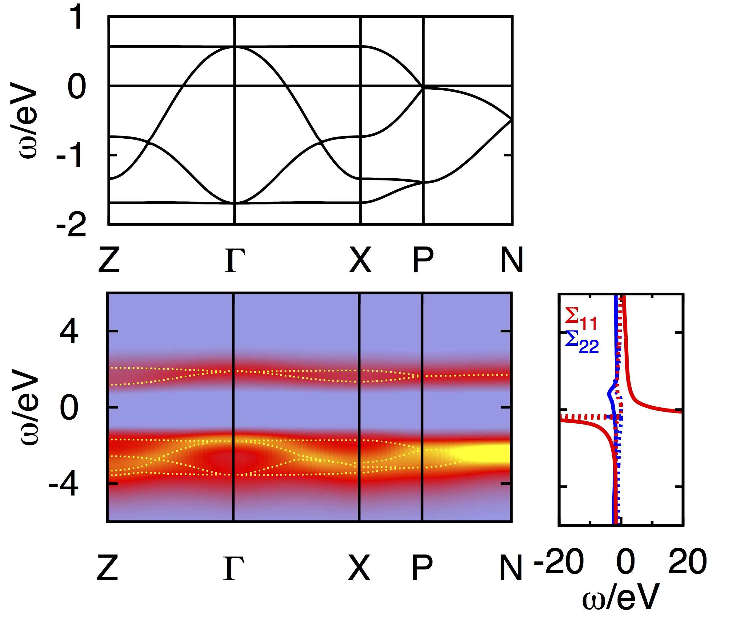
Figure 6: LDA (top) and corresponding LDA+DMFT (bottom) $e_{g}$ band structure of the Mott insulator KCuF₃ in the orbitally ordered phase. Calculations are for the ideal cubic structure, massive downfolding to the $e_{g}$ bands, and for a temperature below the super-exchange orbital-order critical temperature $T_{\rm KK}$. The real part of the self-energy of the hole orbital ($\Sigma_{11}$) diverges in the gap leading to a Mott state. Adapted from Refs. book2011 ; oo1 .

We have up to now not specified the actual size of the LDA Hamiltonian. Wannier functions allow for massive downfolding, i.e., for reducing the Hamiltonian to the minimal basis set describing the correlated electrons. In the example of KCuF₃, considered in the previous section, the smallest possible basis is that made of $e_{g}$ states only. The $e_{g}$ Wannier functions spanning the $e_{g}$ bands are longer ranged than atomic orbitals, because they carry the information on the lattice and the bonding. This can be seen in the orbitals in Fig. 2. The LDA+DMFT band structure for the $e_{g}$ bands is shown in Fig. 6. The advantage of massive downfolding is that the double-counting correction can be incorporated in the chemical potential and does not need to be calculated explicitly. In some cases, however, one has to include non-correlated electrons in the calculation. This is the case if, for example, $p$-$d$ charge-transfer effects play an important role. In these cases a larger basis set is used and the double-counting correction has to be calculated explicitly.

The extension of the LDA+DMFT scheme discussed above to the spin-polarized case (e.g., for studying ferro- or antiferro-magnetic phases) is straightforward, provided that the right unit cells and symmetries are used. The LDA+DMFT scheme can be also easily extended to clusters, e.g., by using a supercell as quantum impurity; other non-local extensions of DMFT are the dynamical-cluster approximation (DCA) dca , the dual-fermion approach, or the GW+DMFT approach (see Refs. book2011 ; book2012 ). One has to keep in mind that increasing the number of sites and degrees of freedom the problem becomes progressively harder; in QMC calculations the computational time becomes quickly prohibitively long and the infamous minus sign problem can arise; in Lanczos-based calculations one might need a computer with more GB of memory than there are atoms in the visible universe. Thus in practice the calculations can reach quickly the feasibility limit, even with the help of modern massively-parallel supercomputers.

As final remark, LDA+DMFT calculations can also be performed charge self-consistently. If we assume that LDA describes uncorrelated electrons sufficiently well, the readjustments in the uncorrelated sector can be calculated by making the total charge density and the reference potential consistent within the LDA, however with the constraints provided by the DMFT solution of the Hubbard model. This requires to work with the full Hamiltonian and, again, to account explicitly for the double-counting correction.

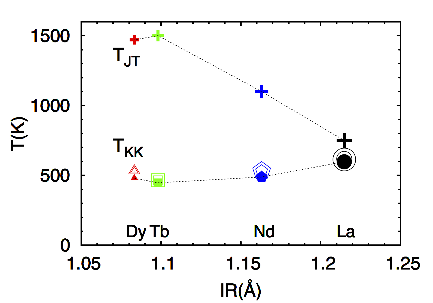
Figure 7: $T_{\rm KK}$, the critical temperature for orbital order due to super-exchange only, versus the experimental orbital melting temperature, $T_{\rm JT}$. Calculations were done with density-density Coulomb interaction (full symbols: HF-QMC; small open symbols: CT-HYB) and full Coulomb interaction (larger open symbols). The results show that spin-flip and pair-hopping terms do not affect $T_{\rm KK}$ in a sizable way. Adapted from Refs. oo2 ; oo3 ; ctqmcflesch .

4 The Origin of Orbital Order

In this paragraph we illustrate a paradigmatic application of the LDA+DMFT technique. Orbital order phenomena play a crucial role in the physics of strongly correlated oxides, such as the $e_{g}$ systems KCuF₃ and LaMnO₃. The origin of orbital order has been therefore debated since long. Two mechanisms have been proposed. The first is electron-phonon coupling ep , which naturally yields a static co-operative Jahn-Teller distortion. The order arises from the splitting of the partially filled degenerate $e_{g}$ levels due to the Jahn-Teller crystal-field. LDA+DMFT calculations have shown that even a small crystal field is sufficient, because it is enhanced by Coulomb repulsion effects; this phenomenon has been observed in very diverse materials d1 ; d2 ; ruthenates . The second mechanism is the purely electronic Kugel-Khomskii super-exchange kk . In this picture the static co-operative Jahn-Teller distortion is a consequence, rather than the cause, of orbital order. In real systems it is very difficult to disentangle the two effects, because both lead to similar co-operative distortions. Total energy studies based on antiferromagnetic LDA+$U$ ldau ; ku and more recently paramagnetic LDA+DMFT leonov calculations show that, in order to explain the presence of the Jahn-Teller co-operative distortion, we have to take into account the Coulomb interaction. However, in both KCuF₃ and LaMnO₃ the magnetic transition temperature ($\sim$40 K for KCuF₃ and $\sim$140 K for LaMnO₃) is sizably smaller than the orbital-ordering temperature, suggesting that quite different mechanisms are involved in the two phenomena.

Recently we devised a procedure which allows us to disentangle the super-exchange from the electron-phonon mechanism oo1 . It consists in performing LDA+DMFT calculations of the orbital polarization versus temperature for a series of progressively less-distorted materials and determining in this way the transition-temperature due to super-exchange only. Using this procedure for KCuF₃ we find $T_{\rm KK}\sim 350~{}$K oo1 . In this system $T_{\rm JT}$, the experimental temperature at which the co-operative Jahn-Teller distortion disappears in X-ray or neutron scattering data, is close or perhaps above the melting temperature ghigna , i.e., $T_{\rm KK}$ is sizable but much smaller than $T_{\rm JT}$. This shows that super-exchange is large but not sufficient to determine the presence of a co-operative Jahn-Teller distortion at high temperatures.

The situation is much more complex for the rare-earth manganites. Figure 7 shows $T_{\rm KK}$ for the $R$MnO₃ series oo2 ; oo3 ; ctqmcflesch , compared to $T_{\rm JT}$. Remarkably, for LaMnO₃ $T_{\rm KK}$ is almost identical to $T_{\rm JT}$. However, $T_{\rm JT}$ has been identified as the temperature at which an orbital order-to-disorder transition occurs melting . The JT distortions have be reported to survive in nano-clusters up to 1150 K clusters . Furthermore, the coincidence $T_{\rm KK}\sim T_{\rm JT}$ only occurs for LaMnO₃. In the rest of the series $T_{\rm KK}$ remains more or less the same, while the experimental $T_{\rm JT}$ becomes as large a 1500 K (Fig. 7). This strongly suggests that super-exchange does not determine the order-to-disorder transition. Finally, we find that tetragonal crystal-field splitting arising from other distortions further reduce the effective $T_{\rm KK}$ oo3 . In conclusion, our results show that in all considered materials, super-exchange effects, although very large, play a small role in the observed melting of orbital order.

5 Conclusions and Outlook

The LDA+DMFT method has opened new horizons for first-principles calculations for strongly correlated system. In the last decades it has proven an extremely successful technique for unraveling the physics of a large variety of strongly correlated materials. It is difficult even to list all its successes so far. A partial overview can be found in reviews georges ; georges2 ; imada ; kotliar , as well as in book2011 . Along the years we have learned that details do matter, for example crystal-fields an order of magnitude smaller than the band width can favor the Mott transition or trigger orbital order d1 ; d2 ; ruthenates ; oo1 .

Electronic structure codes based on LDA+DMFT are slowly becoming available in combination with most popular DFT codes. Modern parallel supercomputers and algorithmic developments are making it possible to solve with DMFT always more complex quantum-impurity models. We can nowadays perform charge-self consistent calculations, optimize structures, calculate phonon spectra and response functions. It is not difficult to imagine that in the not too far future LDA+DMFT codes will become as complex, systematic and general as modern DFT codes.

Important challenges are however still ahead. Non-local effects remain very difficult to describe efficiently. Screening effects are mostly accounted for only at the cLDA or cRPA level. For double-counting corrections only practical recipes exist. To further increase the complexity of the quantum-impurity problem (i.e. to make it more realistic) it is likely that new efficient quantum impurity solvers or even entirely new ideas have to be developed. Perhaps the most important challenge is to identify which details are important for specific classes of problems and systems and to work on the development of optimal schemes to take them all into account.

Appendix

Gaunt coefficients and Coulomb integrals

The two-index Coulomb integrals can be written as

$$U_{m,m^{\prime}} = \sum_{k=0}^{2l}a_{k}^{l}(mm,m^{\prime}m^{\prime})F_{k}=\sum_{k=0}^{2l}b_{k}^{l}(m,m^{\prime})F_{k}^{l},$$

$$J_{m,m^{\prime}} = \sum_{k=0}^{2l}a_{k}^{l}(mm^{\prime},m^{\prime}m)F_{k}=\sum_{k=0}^{2l}c_{k}^{l}(m,m^{\prime})F_{k}^{l},$$

where

$$a_{k}^{l}(m_{\alpha}^{\phantom{\prime}}m^{\prime}_{\alpha},m_{\beta}^{\phantom{\prime}}m_{\beta}^{\prime})=\frac{4\pi}{2k+1}\sum_{q=-k}^{k}\langle lm_{\alpha}^{\phantom{\prime}}|Y^{k}_{q}|lm_{\alpha}^{\prime}\rangle\langle lm_{\beta}^{\phantom{\prime}}|\overline{Y}^{k}_{q}|lm_{\beta}^{\prime}\rangle.$$

In the basis $\{m\}$ of spherical harmonics, the coefficients $G_{k}(m,m^{\prime})=\langle lm|Y^{k}_{q}|lm^{\prime}\rangle$ with $k=2,4$ are given by

$$\begin{array}[]{@{\hspace{3ex}}c@{\hspace{6ex}}c@{\hspace{3ex}}c@{\hspace{6ex}}c}\hskip 12.91663pt\lx@intercol\hfil\displaystyle G_{2}=\frac{1}{7\sqrt{4\pi}}\left[\!\begin{array}[]{rrrrr}-\sqrt{20}&\sqrt{30}&-\sqrt{20}&0&0\\ -\sqrt{30}&\sqrt{5}&\sqrt{5}&-\sqrt{30}&0\\ -\sqrt{20}&-\sqrt{5}&\sqrt{20}&-\sqrt{5}&-\sqrt{20}\\ 0&-\sqrt{30}&\sqrt{5}&\sqrt{5}&-\sqrt{30}\\ 0&0&-\sqrt{20}&\sqrt{30}&-\sqrt{20}\end{array}\!\right]\hfil\hskip 25.83325pt\\[34.44434pt] \hskip 12.91663pt\lx@intercol\hfil\displaystyle G_{4}=\frac{1}{7\sqrt{4\pi}}\left[\!\begin{array}[]{rrrrr}1&-\sqrt{5}&\sqrt{15}&-\sqrt{35}&\sqrt{70}\\ \sqrt{5}&-4&\sqrt{30}&-\sqrt{40}&\sqrt{35}\\ \sqrt{15}&-\sqrt{30}&6&-\sqrt{30}&\sqrt{15}\\ \sqrt{35}&-\sqrt{40}&\sqrt{30}&-4&\sqrt{5}\\ \sqrt{70}&-\sqrt{35}&\sqrt{15}&-\sqrt{5}&1\end{array}\!\right].\hfil\hskip 25.83325pt\end{array}$$

Thus for $l=2$ we have

$$\begin{array}[]{l@{\hspace{5ex}}c@{\hspace{5ex}}c@{\hspace{5ex}}}\displaystyle b_{0}^{2}\!=\!\!\left[\begin{array}[]{r@{\hspace{1ex}}r@{\hspace{1ex}}r@{\hspace{1ex}}r@{\hspace{1ex}}r@{\hspace{1ex}}}1\hskip 4.30554pt&1\hskip 4.30554pt&1\hskip 4.30554pt&1\hskip 4.30554pt&1\hskip 4.30554pt\\ 1\hskip 4.30554pt&1\hskip 4.30554pt&1\hskip 4.30554pt&1\hskip 4.30554pt&1\hskip 4.30554pt\\ 1\hskip 4.30554pt&1\hskip 4.30554pt&1\hskip 4.30554pt&1\hskip 4.30554pt&1\hskip 4.30554pt\\ 1\hskip 4.30554pt&1\hskip 4.30554pt&1\hskip 4.30554pt&1\hskip 4.30554pt&1\hskip 4.30554pt\\ 1\hskip 4.30554pt&1\hskip 4.30554pt&1\hskip 4.30554pt&1\hskip 4.30554pt&1\hskip 4.30554pt\end{array}\right]\hskip 17.22217pt\displaystyle b_{2}^{2}\!=\!\frac{1}{49}\!\left[\begin{array}[]{r@{\hspace{1ex}}r@{\hspace{1ex}}r@{\hspace{1ex}}r@{\hspace{1ex}}r@{\hspace{1ex}}}4\hskip 4.30554pt&-2\hskip 4.30554pt&-4\hskip 4.30554pt&-2\hskip 4.30554pt&4\hskip 4.30554pt\\ -2\hskip 4.30554pt&1\hskip 4.30554pt&2\hskip 4.30554pt&1\hskip 4.30554pt&-2\hskip 4.30554pt\\ -4\hskip 4.30554pt&2\hskip 4.30554pt&4\hskip 4.30554pt&2\hskip 4.30554pt&-4\hskip 4.30554pt\\ -2\hskip 4.30554pt&1\hskip 4.30554pt&2\hskip 4.30554pt&1\hskip 4.30554pt&-2\hskip 4.30554pt\\ 4\hskip 4.30554pt&-2\hskip 4.30554pt&-4\hskip 4.30554pt&-2\hskip 4.30554pt&4\hskip 4.30554pt\end{array}\right]\hfil\hskip 21.52771pt\\ \hfil\hskip 21.52771pt\\ \hskip 17.22217pt\displaystyle b_{4}^{2}\!=\!\frac{1}{49}\frac{1}{9}\!\left[\begin{array}[]{r@{\hspace{1ex}}r@{\hspace{1ex}}r@{\hspace{1ex}}r@{\hspace{1ex}}r@{\hspace{1ex}}}1\hskip 4.30554pt&-4\hskip 4.30554pt&6\hskip 4.30554pt&-4\hskip 4.30554pt&1\hskip 4.30554pt\\ -4\hskip 4.30554pt&16\hskip 4.30554pt&-24\hskip 4.30554pt&16\hskip 4.30554pt&-4\hskip 4.30554pt\\ 6\hskip 4.30554pt&-24\hskip 4.30554pt&36\hskip 4.30554pt&-24\hskip 4.30554pt&6\hskip 4.30554pt\\ -4\hskip 4.30554pt&16\hskip 4.30554pt&-24\hskip 4.30554pt&16\hskip 4.30554pt&-4\hskip 4.30554pt\\ 1\hskip 4.30554pt&-4\hskip 4.30554pt&6\hskip 4.30554pt&-4\hskip 4.30554pt&1\hskip 4.30554pt\end{array}\right]\hfil\hskip 21.52771pt\\ \end{array}$$

$$\begin{array}[]{c@{\hspace{5ex}}c@{\hspace{5ex}}c@{\hspace{5ex}}}\displaystyle c_{0}^{2}\!=\!\!\left[\begin{array}[]{r@{\hspace{1ex}}r@{\hspace{1ex}}r@{\hspace{1ex}}r@{\hspace{1ex}}r@{\hspace{1ex}}}1\hskip 4.30554pt&0\hskip 4.30554pt&0\hskip 4.30554pt&0\hskip 4.30554pt&0\hskip 4.30554pt\\ 0\hskip 4.30554pt&1\hskip 4.30554pt&0\hskip 4.30554pt&0\hskip 4.30554pt&0\hskip 4.30554pt\\ 0\hskip 4.30554pt&0\hskip 4.30554pt&1\hskip 4.30554pt&0\hskip 4.30554pt&0\hskip 4.30554pt\\ 0\hskip 4.30554pt&0\hskip 4.30554pt&0\hskip 4.30554pt&1\hskip 4.30554pt&0\hskip 4.30554pt\\ 0\hskip 4.30554pt&0\hskip 4.30554pt&0\hskip 4.30554pt&0\hskip 4.30554pt&1\hskip 4.30554pt\end{array}\right]\hskip 17.22217pt\displaystyle c_{2}^{2}\!=\!\frac{1}{49}\!\left[\begin{array}[]{r@{\hspace{1ex}}r@{\hspace{1ex}}r@{\hspace{1ex}}r@{\hspace{1ex}}r@{\hspace{1ex}}}4\hskip 4.30554pt&6\hskip 4.30554pt&4\hskip 4.30554pt&0\hskip 4.30554pt&0\hskip 4.30554pt\\ 6\hskip 4.30554pt&1\hskip 4.30554pt&1\hskip 4.30554pt&6\hskip 4.30554pt&0\hskip 4.30554pt\\ 4\hskip 4.30554pt&1\hskip 4.30554pt&4\hskip 4.30554pt&1\hskip 4.30554pt&4\hskip 4.30554pt\\ 0\hskip 4.30554pt&6\hskip 4.30554pt&1\hskip 4.30554pt&1\hskip 4.30554pt&6\hskip 4.30554pt\\ 0\hskip 4.30554pt&0\hskip 4.30554pt&4\hskip 4.30554pt&6\hskip 4.30554pt&4\hskip 4.30554pt\end{array}\right]\hskip 17.22217pt\displaystyle c_{4}^{2}\!=\!\frac{1}{49}\frac{1}{9}\!\left[\begin{array}[]{r@{\hspace{1ex}}r@{\hspace{1ex}}r@{\hspace{1ex}}r@{\hspace{1ex}}r@{\hspace{1ex}}}1\hskip 4.30554pt&5\hskip 4.30554pt&15\hskip 4.30554pt&35\hskip 4.30554pt&70\hskip 4.30554pt\\ 5\hskip 4.30554pt&16\hskip 4.30554pt&30\hskip 4.30554pt&40\hskip 4.30554pt&35\hskip 4.30554pt\\ 15\hskip 4.30554pt&30\hskip 4.30554pt&36\hskip 4.30554pt&30\hskip 4.30554pt&15\hskip 4.30554pt\\ 35\hskip 4.30554pt&40\hskip 4.30554pt&30\hskip 4.30554pt&16\hskip 4.30554pt&5\hskip 4.30554pt\\ 70\hskip 4.30554pt&35\hskip 4.30554pt&15\hskip 4.30554pt&5\hskip 4.30554pt&1\hskip 4.30554pt\end{array}\right]\hfil\hskip 21.52771pt\end{array}$$

Instead, in the basis of real harmonics, the coefficients become

$$\begin{array}[]{l@{\hspace{5ex}}c@{\hspace{5ex}}c@{\hspace{5ex}}}\displaystyle b_{0}^{2}\!=\!\!\left[\begin{array}[]{r@{\hspace{1ex}}r@{\hspace{1ex}}r@{\hspace{1ex}}r@{\hspace{1ex}}r@{\hspace{1ex}}}1\hskip 4.30554pt&1\hskip 4.30554pt&1\hskip 4.30554pt&1\hskip 4.30554pt&1\hskip 4.30554pt\\ 1\hskip 4.30554pt&1\hskip 4.30554pt&1\hskip 4.30554pt&1\hskip 4.30554pt&1\hskip 4.30554pt\\ 1\hskip 4.30554pt&1\hskip 4.30554pt&1\hskip 4.30554pt&1\hskip 4.30554pt&1\hskip 4.30554pt\\ 1\hskip 4.30554pt&1\hskip 4.30554pt&1\hskip 4.30554pt&1\hskip 4.30554pt&1\hskip 4.30554pt\\ 1\hskip 4.30554pt&1\hskip 4.30554pt&1\hskip 4.30554pt&1\hskip 4.30554pt&1\hskip 4.30554pt\end{array}\right]\hskip 8.61108pt\displaystyle b_{2}^{2}\!=\!\frac{1}{49}\!\left[\begin{array}[]{r@{\hspace{1ex}}r@{\hspace{1ex}}r@{\hspace{1ex}}r@{\hspace{1ex}}r@{\hspace{1ex}}}4\hskip 4.30554pt&-2\hskip 4.30554pt&-4\hskip 4.30554pt&-2\hskip 4.30554pt&4\hskip 4.30554pt\\ -2\hskip 4.30554pt&4\hskip 4.30554pt&2\hskip 4.30554pt&-2\hskip 4.30554pt&-2\hskip 4.30554pt\\ -4\hskip 4.30554pt&2\hskip 4.30554pt&4\hskip 4.30554pt&2\hskip 4.30554pt&-4\hskip 4.30554pt\\ -2\hskip 4.30554pt&-2\hskip 4.30554pt&2\hskip 4.30554pt&4\hskip 4.30554pt&-2\hskip 4.30554pt\\ 4\hskip 4.30554pt&-2\hskip 4.30554pt&-4\hskip 4.30554pt&-2\hskip 4.30554pt&4\hskip 4.30554pt\end{array}\right]\hfil\hskip 21.52771pt\\ \hfil\hskip 21.52771pt\\ \hskip 8.61108pt\displaystyle b_{4}^{2}\!=\!\frac{1}{49}\frac{1}{9}\!\left[\begin{array}[]{r@{\hspace{1ex}}r@{\hspace{1ex}}r@{\hspace{1ex}}r@{\hspace{1ex}}r@{\hspace{1ex}}}36\hskip 4.30554pt&-4\hskip 4.30554pt&6\hskip 4.30554pt&-4\hskip 4.30554pt&-34\hskip 4.30554pt\\ -4\hskip 4.30554pt&36\hskip 4.30554pt&-24\hskip 4.30554pt&-4\hskip 4.30554pt&-4\hskip 4.30554pt\\ 6\hskip 4.30554pt&-24\hskip 4.30554pt&36\hskip 4.30554pt&-24\hskip 4.30554pt&6\hskip 4.30554pt\\ -4\hskip 4.30554pt&-4\hskip 4.30554pt&-24\hskip 4.30554pt&36\hskip 4.30554pt&-4\hskip 4.30554pt\\ -34\hskip 4.30554pt&-4\hskip 4.30554pt&6\hskip 4.30554pt&-4\hskip 4.30554pt&36\hskip 4.30554pt\end{array}\right]\hfil\hskip 21.52771pt\end{array}$$

$$\begin{array}[]{c@{\hspace{5ex}}c@{\hspace{5ex}}c@{\hspace{5ex}}}\displaystyle c_{0}^{2}\!=\!\!\left[\begin{array}[]{r@{\hspace{1ex}}r@{\hspace{1ex}}r@{\hspace{1ex}}r@{\hspace{1ex}}r@{\hspace{1ex}}}1\hskip 4.30554pt&0\hskip 4.30554pt&0\hskip 4.30554pt&0\hskip 4.30554pt&0\hskip 4.30554pt\\ 0\hskip 4.30554pt&1\hskip 4.30554pt&0\hskip 4.30554pt&0\hskip 4.30554pt&0\hskip 4.30554pt\\ 0\hskip 4.30554pt&0\hskip 4.30554pt&1\hskip 4.30554pt&0\hskip 4.30554pt&0\hskip 4.30554pt\\ 0\hskip 4.30554pt&0\hskip 4.30554pt&0\hskip 4.30554pt&1\hskip 4.30554pt&0\hskip 4.30554pt\\ 0\hskip 4.30554pt&0\hskip 4.30554pt&0\hskip 4.30554pt&0\hskip 4.30554pt&1\hskip 4.30554pt\end{array}\right]\hskip 17.22217pt\displaystyle c_{2}^{2}\!=\!\frac{1}{49}\!\left[\begin{array}[]{r@{\hspace{1ex}}r@{\hspace{1ex}}r@{\hspace{1ex}}r@{\hspace{1ex}}r@{\hspace{1ex}}}4\hskip 4.30554pt&3\hskip 4.30554pt&4\hskip 4.30554pt&3\hskip 4.30554pt&0\hskip 4.30554pt\\ 3\hskip 4.30554pt&4\hskip 4.30554pt&1\hskip 4.30554pt&3\hskip 4.30554pt&3\hskip 4.30554pt\\ 4\hskip 4.30554pt&1\hskip 4.30554pt&4\hskip 4.30554pt&1\hskip 4.30554pt&4\hskip 4.30554pt\\ 3\hskip 4.30554pt&3\hskip 4.30554pt&1\hskip 4.30554pt&4\hskip 4.30554pt&3\hskip 4.30554pt\\ 0\hskip 4.30554pt&3\hskip 4.30554pt&4\hskip 4.30554pt&3\hskip 4.30554pt&4\hskip 4.30554pt\end{array}\right]\hskip 17.22217pt\displaystyle c_{4}^{2}\!=\!\frac{1}{49}\frac{1}{9}\!\left[\begin{array}[]{r@{\hspace{1ex}}r@{\hspace{1ex}}r@{\hspace{1ex}}r@{\hspace{1ex}}r@{\hspace{1ex}}}36\hskip 4.30554pt&20\hskip 4.30554pt&15\hskip 4.30554pt&20\hskip 4.30554pt&35\hskip 4.30554pt\\ 20\hskip 4.30554pt&36\hskip 4.30554pt&30\hskip 4.30554pt&20\hskip 4.30554pt&20\hskip 4.30554pt\\ 15\hskip 4.30554pt&30\hskip 4.30554pt&36\hskip 4.30554pt&30\hskip 4.30554pt&15\hskip 4.30554pt\\ 20\hskip 4.30554pt&20\hskip 4.30554pt&30\hskip 4.30554pt&36\hskip 4.30554pt&20\hskip 4.30554pt\\ 35\hskip 4.30554pt&20\hskip 4.30554pt&15\hskip 4.30554pt&20\hskip 4.30554pt&36\hskip 4.30554pt\end{array}\right]\hfil\hskip 21.52771pt\end{array}$$

The transformation matrix $M$ from spherical to real harmonics is

$$\begin{array}[]{c@{\hspace{5ex}}c@{\hspace{6ex}}cc@{\hspace{5ex}}c@{\hspace{6ex}}c}\hfil\hskip 21.52771pt&\displaystyle M=\frac{1}{\sqrt{2}}\left[\begin{array}[]{r@{\hspace{1ex}}r@{\hspace{1ex}}r@{\hspace{1ex}}r@{\hspace{1ex}}r@{\hspace{1ex}}}-i\hskip 4.30554pt&0\hskip 4.30554pt&0\hskip 4.30554pt&0\hskip 4.30554pt&i\hskip 4.30554pt\\ 0\hskip 4.30554pt&i\hskip 4.30554pt&0\hskip 4.30554pt&i\hskip 4.30554pt&0\hskip 4.30554pt\\ 0\hskip 4.30554pt&0\hskip 4.30554pt&\sqrt{2}\hskip 4.30554pt&0\hskip 4.30554pt&0\hskip 4.30554pt\\ 0\hskip 4.30554pt&-1\hskip 4.30554pt&0\hskip 4.30554pt&1\hskip 4.30554pt&0\hskip 4.30554pt\\ 1\hskip 4.30554pt&0\hskip 4.30554pt&0\hskip 4.30554pt&0\hskip 4.30554pt&1\hskip 4.30554pt\\ \end{array}\right].\hfil\hskip 25.83325pt\end{array}$$

The Coulomb integrals can also be expressed as linear combination of Racah parameters; for the $d$ shell the latter are

$$A = F_{0}-\frac{49}{441}F_{4}\quad\quad B=\frac{1}{49}F_{2}-\frac{5}{441}F_{4}\quad\quad C=\frac{35}{441}F_{4}.$$

References

• (1) W. Kohn, Nobel Lecture: Electronic structure of matter wave functions and density functionals, Rev. Mod. Phys. 71, 1253 (1998)
• (2) U. von Barth, Physica Scripta 109, 9 (2004)
• (3) R.M. Martin, Electronic Structure, Basic Theory and Practical Methods
(Cambridge University Press, 2004)
• (4) A.C. Hewson, The Kondo Problem to Heavy Fermions
(Cambridge University Press, 1993)
See, e.g., ”The possibility of First Principles Calculations?”
• (5) W. Metzner and D. Vollhardt, Phys. Rev. Lett. 62, 324 327 (1989)
A. Georges and G. Kotliar, Phys. Rev. B 45, 6479 (1992)
• (6) A. Georges, G. Kotliar, W. Krauth, and M.J. Rozenberg, Rev. Mod. Phys. 68, 13 (1996)
• (7) V.I. Anisimov, A.I. Poteryaev, M.A. Korotin, A.O. Anokhin, and G. Kotliar,
J. Phys: Condens. Matter 9, 7359 (1997);
A.I. Lichtenstein and M.I. Katsnelson, Phys. Rev. B 57, 6884 (1998)
• (8) E. Pavarini, E. Koch, A. Lichtenstein, D. Vollhardt (eds.)
The LDA+DMFT approach to strongly correlated materials,
Reihe Modeling and Simulation, Vol. 1
(Forschungszentrum Jülich, 2011) http://www.cond-mat.de/events/correl11
• (9) E. Pavarini, E. Koch, F. Anders, M. Jarrell (eds.)
Correlated electrons: from models to materials,
Reihe Modeling and Simulation, Vol. 2
(Forschungszentrum Jülich, 2012) http://www.cond-mat.de/events/correl12
• (10) E. Pavarini, The LDA+DMFT approach, in Ref. book2011
• (11) A. Georges, in Lectures on the Physics of Highly Correlated Electron Systems VIII, American Institute of Physics Conference Proceedings 715, 3 (2004)
• (12) H. Hafermann, F. Lechermann, A.I. Rubtsov, M.I. Katsnelson and A.I. Lichtenstein, in D.C. Cabra, A. Honecker, and P. Pujol (eds),
Many-body theories of Many-Particle in Condensed Matter Physics, Springer Verlag (Berlin Heidelberg, 2012)
• (13) M. Imada and T. Miyake, J. Phys. Soc. Jpn. 79, 112001 (2010)
• (14) G. Kotliar, S.Y. Savrasov, K. Haule, V.S. Oudovenko, O. Parcollet and C.A. Marianetti,
Rev. Mod. Phys. 78, 865 (2006)
• (15) E. Pavarini, A. Yamasaki, J. Nuss and O.K. Andersen, New J. Phys. 7, 188 (2005)
• (16) O.K. Andersen, NMTOs and their Wannier Functions, in Ref. book2011
• (17) N. Marzari and D. Vanderbilt, Phys. Rev. B 56, 12847 (1997)
• (18) B. Amadon, F. Lechermann, A. Georges, F. Jollet, T.O. Wehling, and A.I. Lichtenstein,
Phys. Rev. B 77, 205112 (2008)
• (19) V.I. Anisimov, F. Aryasetiawan and A.I. Lichtenstein, J. Phys. Cond. Mat. 9, 767 (1997)
• (20) O. Gunnarsson, O.K. Andersen, O. Jepsen and J. Zaanen, Phys. Rev. B 37, 1708 (1989)
• (21) F. Aryasetiawan, M. Imada, A. Georges, G. Koliar, S. Biermann, and A.I. Lichtenstein, Phys. Rev. B 70, 195104 (2004)
• (22) G. Zhang, E. Gorelov, E. Koch and E. Pavarini, Phys. Rev. B 86, 184413 (2012)
• (23) J.E. Hirsch and R.M. Fye, Phys. Rev. Lett. 56, 2521 (1986)
• (24) E. Gull, A.J. Millis, A.I. Lichtenstein, A.N. Rubtsov, M. Troyer and P. Werner,
Rev. Mod. Phys. 83, 349 (2011)
• (25) M. Caffarel, W. Krauth, Phys. Rev. Lett. 72, 1545 (1994)
E. Koch, G. Sangiovanni, and O. Gunnarsson, Phys. Rev. B 78, 115102 (2008)
• (26) E. Koch, The Lanczos Method, in Ref. book2011
• (27) M. Jarrell, The Maximum Entropy Method, in Ref. book2012 .
• (28) A. Mishchenko, Stochastic Optimization for Analytical Continuation: When a priori Knowledge is Missing, in Ref. book2012
• (29) T. Maier, M. Jarrell, T. Pruschke, and M. Hettler, Rev. Mod. Phys. 77, 1027 (2005)
• (30) K.I. Kugel and D.I. Khomskii,
Zh. Eksp. Teor. Fiz. 64, 1429 (1973) [Sov. Phys. JETP 37, 725 (1973)]
• (31) J. Kanamori, J. Appl. Phys. 31, S14 (1960)
• (32) E. Pavarini, S. Biermann, A. Poteryaev, A.I. Lichtenstein, A. Georges and O. K. Andersen, Phys. Rev. Lett. 92, 176403 (2004)
• (33) M. De Raychaudhury, E. Pavarini and O.K. Andersen,
Phys. Rev. Lett. 99, 126402 (2007)
• (34) E. Gorelov, M. Karolak, T. O. Wehling, F. Lechermann, A.I. Lichtenstein and E. Pavarini,
Phys. Rev. Lett. 104, 226401 (2010)
• (35) W. G. Yin, D. Volja, and W. Ku, Phys. Rev. Lett. 96, 116405 (2006)
• (36) I. Leonov, N. Binggeli, Dm. Korotin, V.I. Anisimov, and D. Vollhardt,
Phys. Rev. Lett. 101, 096405 (2008)
I. Leonov, Dm. Korotin, N. Binggeli, V.I. Anisimov, and D. Vollhardt,
Phys. Rev. B 81, 075109 (2010)
• (37) P. Ghigna, S. Marco, C. Mazzoli, M. Brunelli, C. Laurenti, and C. Ferrero,
Phys. Rev. B 81, 073107 (2010)
L.G. Marshall, J. Zhou, J. Zhang, J. Han, S.C. Vogel, X. Yu, Y. Zhao, M.T. Fernández-Díaz, J. Cheng, and J.B. Goodenough, Phys. Rev. B 87, 014109 (2013)
• (38) E. Pavarini, E. Koch and A.I. Lichtenstein, Phys. Rev. Lett. 101, 266405 (2008)
• (39) E. Pavarini and E. Koch, Phys. Rev. Lett. 104, 086402 (2010)
• (40) A. Flesch, G. Zhang, E. Koch and E. Pavarini, Phys. Rev. B 85, 035124 (2012)
• (41) A. Flesch, E. Gorelov, E. Koch, E. Pavarini, Phys. Rev. B 87, 195141 (2013)
• (42) M.C. Sánchez, G. Subías, J. García, and J. Blasco, Phys. Rev. Lett. 90, 045503 (2003)
• (43) J. Rodríguez-Carvajal, M. Hennion, F. Moussa, A.H. Moudden, L. Pinsard,
and A. Revcolevschi, Phys. Rev. B 57 R3189 (1998)
J.-S. Zhou and J.B. Goodenough, Phys. Rev. B 68, 144406 (2003)
and Phys. Rev. Lett. 96, 247202 (2006)