Uncertainty in climate science and climate policy

1 Introduction

This essay, written by a statistician and a climate scientist, describes our view of the gap that exists between current practice in mainstream climate science, and the practical needs of policymakers charged with exploring possible interventions in the context of climate change. By ‘mainstream’ we mean the type of climate science that dominates in universities and research centres, which we will term ‘academic’ climate science, in contrast to ‘policy’ climate science; aspects of this distinction will become clearer in what follows.

In a nutshell, we do not think that academic climate science equips climate scientists to be as helpful as they might be, when involved in climate policy assessment. Partly, we attribute this to an over-investment in high resolution climate simulators, and partly to a culture that is uncomfortable with the inherently subjective nature of climate uncertainty.

In section 2 we discuss current practice in academic climate science, in relation to the needs of policymakers. Section 3 addresses the aparently common misconception (among climate scientists) that uncertainty is something ‘out there’ to be quantified, much like the strength of meridional overturning circulation. Section 4, the heart of the essay, addresses the core needs of the policymaker, and focuses on three strictures for the climate scientist wanting to help her: answer the question, own the judgement, and be coherent. Section 5 concludes with a brief reflection.

We have taken the opportunity in this essay to be a little more polemical than we might be in an academic paper, and maybe a little more exuberent in our expressions. We have also ignored the technical details of practical climate science, something we are both involved in day-to-day, choosing instead to look at the larger picture. We believe that our observations are valid more widely than just climate science; for example many of them would apply with little modification in many areas of natural hazards, and in radiological or ecotoxicological risk assessment (Rougier et al., 2013). But they seem most pertinent in climate science, which outstrips the other areas in terms of funding. For example, the UK’s Natural Environment Research Council (NERC), whose vision is to “advance knowledge and understanding of the Earth and its environments to help secure a sustainable future for the planet and its people”, allocates $40\%$ of its science budget to climate science and earth system science (NERC Annual Report and Accounts 2010–11, p. 40).

2 Different modes of climate science

For our purposes, the telling feature of climate science is that it gained much of its momentum in the era before climate change became a pressing societal concern. Consequently, when policymakers turned to climate science for advice, they encountered a well-developed academic field whose focus was more towards explanation than prediction. Explanation, in this context, is verifying that observable regularities in the climate system are emergent properties of the basic physics. Largely this is through the interplay between observation and dynamical climate simulation. As the resolution of climate simulators increases, more observed regularities fall into the ‘explained’ category. The El Niño Southern Oscillation (ENSO) is getting closer to falling into this category, for example (Guilyardi et al., 2009).

Thus for investment, the dominant vector in academic climate science has been to improve the spatial and temporal resolution of the solvers in climate simulators. Supporting evidence can be found in meteorology. It is argued that one of the contributory factors to measurable improvements in weather forecasting over the last thirty years is higher-resolution solvers, although the quantification of this is confounded by simultaneous improvements in understanding the physics, in the amount of data available for calibration, and in techniques for data assimilation (Kalnay, 2002, ch. 1). Setting these confounders aside, it seems natural to assert that higher resolution solvers will lead to better climate simulators. And indeed, we would not deny this, but we would also question whether in fact it is resolution that is limiting the fidelity of climate simulators.

The reason that we are suspicious of arguments about climate founded on experiences in meteorology is the presence of biological and chemical processes in the earth system that operate on climate policy but not weather time-scales. We believe that the acknowledgement of biogeochemistry as a full part of the climate system distinguishes the true climate scientist from the converted meteorologist. Our lack of understanding of climate’s critical ecosystems mocks the precision with which we can write down and approximate the Navier-Stokes equations. The problem is, though, that putting ecosystems into a climate simulator is a huge challenge, and progress is difficult to quantify. It introduces more uncertain parameters, and, by replacing prescribed fields with time-evolving fields, it can actually make the performance of the simulator worse, until tuning is successfully completed (and there is no guarantee of success). Newman (2011) provides a short and readable account of the difficulties of biology, in comparison to physics.

On the other hand, spending money on higher resolution solvers requires fewer parameterisations of sub-grid-scale processes, and so reduces the challenge of tuning. This activity has a well-documented provenance, and a clear motivation within a coherent science plan. And we cannot resist pointing out another immediate benefit: one can show the funder a more realistic looking ocean simulation (“Now at $0.5^{\circ}$ resolution!”)—although in fact resolutions as high as $0.1^{\circ}$ do not fool experienced oceanographers. But while this push to higher resolutions is natural for meteorology, with its forecast horizon measured in days, for climate we fear that it blurs the distinction between what one can simulate, and what one ought to simulate for policy purposes.

So how might the investment be directed differently? For climate policy it is necessary to enumerate what might happen under different climate interventions: do nothing, monetise carbon, regulation for contraction and convergence, geo-engineering, and so on. And each of these interventions must be evaluated for a range of scenarios that capture future uncertainty about technology, economics, and demographics. For each pair of intervention and scenario there is a range of possible outcomes, which represent our uncertainty about future climate. Uncertainty here is ‘total uncertainty’: only the intervention and the scenario are specified—the policymaker does not have the luxury of being able to pick and choose which uncertainties are incorporated and which are ignored.

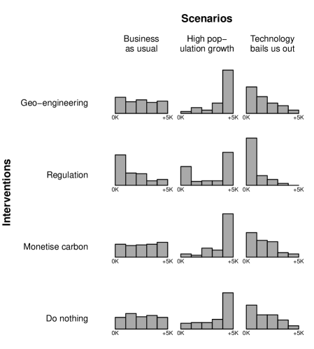
Figure 1: Policy tableau, showing the effect of different possible interventions under different scenarios. These frequency histograms might in this case measure simulated global warming by 2100 under different not-implausible simulator configurations, but more generally they would measures losses, inferred from simulated distributions for weather in 2100. Please note that these histograms are completely fictitious!

Internal variability, part of the natural variability of the climate system, can be estimated from high-resolution simulators, but it is only a tiny part of total uncertainty. Over centurial scales, it is negligible compared to our combined uncertainty of the behaviour of the ice-sheets, and the marine and terrestrial biosphere. This uncertainty can be assessed with the assistance of climate simulators, if it is possible to run them repeatedly under different configurations of the simulator parameters and modules, where these configurations attempt to span the range of not-implausible climate system behaviours. To construct a tableau such as the one in Figure 1 will require a minimum of $4\times 3\times 100\times 90$ models-years of simulation, say 120,000 model-years, including spin-up. The $100$ is the number of different simulator configurations that might be tried, and the $90$ is the number of years until 2100. Of course, $100$ is woefully small for the number of configurations. There are more than one hundred uncertain parameters in a high-resolution climate simulator (Murphy et al., 2004). Admittedly only some of these will turn out to be important but we cannot rule out interactions among the parameters. There is a well-developed statistical field for this type of analysis, see, e.g., Santner et al. (2003).

Note that this is a designed experiment, deliberately constructed to be informative about uncertainty. It is completely different from assembling an ad hoc collection of simulator runs, such as the CMIP3 or CMIP5 multimodel ensembles, in the same way that a carefully stratified sample of $100$ people is far more informative about a population than simply selecting the next $100$ people that pass a particular lamp-post. In the absence of designed experiments, though, climate scientists who want to assess uncertainty will have to use the ad hoc ensemble. The various types and uses of currently-available ensembles of climate simulator runs are reviewed in Parker (2010) and Murphy et al. (2011).

So what is the status of these policy-relevant designed experiments? Current ‘IPCC class’ simulators (with a solver resolution of about $1^{\circ}$) run at about 100 model-years per month of wall-clock time. So starting now, an experiment to assess uncertainty in 2100 for policy purposes will be finished in about 100 years, if it is performed at one research centre. But this might be reduced to 10 years if the runs were shared out across all centres, or even less factoring in faster computers and no increase in resolution. Thus these IPCC class simulators could be very helpful for assessing uncertainty and supporting policymakers, but this requires a cap on solver resolution, and careful coordination across research centres. In contrast, the current uncoordinated approach, with its apparent commitment to spending CPU cycles on a few runs of high-resolution climate simulators, will force climate scientists in 2020 to base their future climate assessments on ad hoc ensembles.

3 The nature of uncertainty about climate

In this paper we confine our discussion of climate uncertainty quantification to the assessment of probabilities. There are, of course, several interpretations of probability. L.J. Savage wrote of “dozens” of different interpretations of probability Savage (1954, p. 2), and he focused on three main strands: the Objective (or Frequentist), the Personalistic, and the Necessary. This tripartite classification is widely accepted among statisticians, and discussed, with embellishments, in the initial chapters of Walley (1991) and Lad (1996). Not to be outdone, Hájek (2012) notes that philosophers of probability now have six leading interpretations of probability.

Of all of these interpretations, however, we contend that only the Personalistic interpretation can capture the ‘total uncertainty’ inherent in the assessment of climate policy. Our uncertainty about future climate is predominantly epistemic uncertainty—the uncertainty that follows from limitations in knowledge and resources. The hallmark of epistemic uncertainty is that it could, in principle, be reduced with further introspection, or further experiments. As one of the key drivers of research investment in climate science is to reduce uncertainty, this epistemic interpretation of ‘total uncertainty’ must be uncontentious. It rules out the Objective (classical, frequency, propensity) interpretation, and leaves us with Personalistic and Necessary (also termed logical) interpretations.

The Necessary interpretation asserts that there are principles of reasoning that extend Boolean logic to uncertainty, and that these principles are in fact the calculus of probability and Bayesian conditioning. This interpretation is formally attractive, but invokes additional principles to ‘fill in’ those initial probabilities that are mandated by conditioning—which are generally referred to as ‘prior’ probabilities in a Bayesian context. These are to be based on self-evident properties of the inference, such as symmetries. Examples are discussed in Jaynes (2003); see, for example, his elegant resolution of Bertrand’s problem (sec. 12.4.4). However, it is hard to know how one might discover and apply these properties in an assessment of, say, the maximum height of the water in the Thames Estuary in 2100. Thus, starting with Frank Ramsey, and finding eloquent champions in Bruno de Finetti and L.J. Savage, among others, the Personalistic interpretation has provided an operational subjective definition of probability, in terms of betting rates (see, e.g. Ramsey, 1931; de Finetti, 1964; Savage, 1954; Savage et al., 1962). De Finetti’s late writings are both subtle and discursive; Lad (1996) attempts to corral them.

Not everyone will find the Personalistic definition of probability compelling. But at least it provides a very clear answer to the question “What do You mean when You state that $\Pr(A)=p$?” A brief answer is that, if betting for a small amount of money, such as $\pounds 1$, You would be agreeable to staking up to $\pounds p$ in a gamble to receive $\pounds 1$ if $A$ turns out to be true and nothing if $A$ turns out to be false. There are other operationalisations as well, which are very similar but not psychologically equivalent; see, e.g., the discussion in Goldstein and Wooff (2007, sec. 2.2). Our view is that an operationalisation of Personalistic probability is highly desirable, and a useful thing to fall back on, but not in itself the yardstick by which all probabilities are assessed. But, if someone provides a probability $p$ for a proposition $A$, it might be a good idea to ask him if he would be prepared to bet $\pounds p$ on $A$ being true: the answer could be very revealing.

However, many physical scientists seem to be very uncomfortable with the twin notions that uncertainty is subjective (i.e. it is a property of the mind), and that probabilities are expressions of personal inclinations to act in certain ways. At least part of the problem concerns the use of the word ‘subjective’, about which the first author has written before (Rougier, 2007, sec. 2). This word is clearly inflammatory. We suggest that some scientists have confused the Mertonian scientific norm of ‘disinterestedness’ with the notion of ‘objectivity’, and then taken subjectivity to be the antithesis of objectivity, and thus to be avoided at all costs. L.J. Savage was sensitive to this confusion and hence favoured ‘Personalistic’. De Finetti strongly favoured ‘subjective’, about which Jeffrey (2004, p. 76, footnote 1) commented on “the lifelong pleasure that de Finetti found in being seen to give the finger to the establishment”.

Confusion about ‘subjectivity’ is just a digression, though. What is abundantly clear is that climate scientists are not ready to accept that climate uncertainties are Personalistic. Their every reference to ‘the uncertainty’ commits an error which the physicist E.T. Jaynes called the ‘mind projection fallacy’:

an almost universal tendency to disguise epistemological statements by putting them into a grammatical form which suggests to the unwary an ontological statement. To interpret the first kind of statement in the ontological sense is to assert that one’s own private thoughts and sensations are realities existing externally in Nature. (Jaynes, 2003, p. 22).

Jaynes is an example of a physicist who embraced the essential subjectivity of uncertainty: he advocated the Necessary interpretation, plus the additional principle of maximising Shannon entropy to extend limited judgements to probabilities. Paris (1994) provides a detailed assessment of the properties of this entropy-maximising approach, among others.

One very stealthy manifestation of the Mind Projection Fallacy is the substitution of ‘assumptions’ for ‘judgements’ when discussing uncertainty. Assumptions typically refer to simplifications we assert about the system itself. It is perfectly acceptable to assume that, for example, the hydrostatic approximation holds: this is a statement that actual ocean behaves a lot like a slightly different ocean that is much simpler to analyse. You cannot assume, though, that the maximum water level in the Thames Estuary in 2100 has a Gaussian distribution. Instead, You may judge it appropriate to represent Your uncertainty about the maximum water level with a Gaussian distribution. This is rather wordy, unfortunately, which is perhaps why it is so easy to lapse in this way.

Consider the uncertainty assessment guidelines for the forthcoming IPCC report (Mastrandrea et al., 2010). Nowhere in the guidelines was it thought necessary to define ‘probability’. Either the authors of the guidelines were not aware that this concept was amendable to several different interpretations, or that they were aware of this, and decided against bringing it out into the open. One can imagine, for example, that an opening statement of the form “In the context of climate prediction, probability is an expression of subjective uncertainty and it can be quantified with reference to a subject’s betting behaviour” would have caused great consternation—so much the better!

We can hardly suppose that the omission of a definition for the key concept in such an important and high-profile document was made in ignorance. And yet the mind projection fallacy is in evidence throughout. It looks as though the authors have deliberately chosen not to acknowledge the essential subjectivity of climate uncertainty, and to suppress linguistic usage that would indicate otherwise. This should be termed ‘monster denial’ in the taxonomy of Curry and Webster (2011). Choosing not to rock the boat is convenient for academic climate scientists. But it makes life difficult for policymakers, who are tasked with turning uncertainties into actions. For policymakers, the meaning of ‘$\Pr(A)=p$’ is of paramount importance, and they need to know if ten different climate scientists mean it ten different ways.

4 The risk manager’s point of view

In any discussion of uncertainty and policy it is helpful to label the key players (Smith, 2010, ch. 1). Conventionally, the person who selects the intervention is the risk manager, who represents a particular set of stakeholders. These stakeholders, who are funding the risk manager, and will also fund the intervention that she selects, will appoint an auditor, whom the risk manager must satisfy. This framework, of a risk manager who must satisfy an auditor, is a simple way to abstract from the complexities of any particular decision. It emphasises that the risk manager is an agent who must defend her selection, and this has important consequences for the way in which she acts.

The risk manager is surely uncertain about future climate, and its implications. For concreteness, suppose that her concern is about the maximum height of water in the Thames Estuary in the year 2100. If asked, she might say, “Really, I’ve no idea, perhaps not lower than today’s value, and not more than two metres higher.” But she is not obliged to make such an assessment in isolation: she can consult an expert. Put simply, her expert is someone whose judgements she accepts as her own (see Lad, 1996, sec. 6.3 for a discussion). So one task of the risk manager is to select her expert, and she must do this in such a way that the auditor is satisfied with the selection process, and with the elicitation process. When seen from the other side, it follows that scientists who want to be involved in climate policy are competing with each other to be selected as one of the risk manager’s experts. Therefore they must demonstrate their grasp of the risk manager’s needs. Likewise, for climate scientists who are competing for policy-tagged funding.

We highlight the following three risk managers’ needs, as posing particular challenges for academic climate scientists.

4.1 Answer the question

As already discussed, the risk manager needs an assessment of ‘total uncertainty’. It can be difficult for the climate scientist to assess his total uncertainty about future climate because of academic climate science’s focus on consuming CPU cycles in higher-resolution solvers, rather than designed replications across alternative not-implausible configurations of simulator parameters and modules. This leaves the willing-to-engage climate scientist ill-equipped to answer questions about ranges for future climate values, because he has nothing other than intuition to guide him on the consequence of the limitations in our knowledge. Unfortunately, his intuition may be tentative at best when reasoning about a dynamical system as complex as the climate system, on centurial timescales.

In this case, the climate scientist may end up specifying very wide intervals which, although honest, do not advance the risk manager because they swamp any ‘treatment effect’ that might arise from different choices of intervention. This honest climate scientist may well be passed over in favour of other experts who advertise their smaller uncertainty as a putative measure of their superior expertise. This type of competition is extensively discussed in Tetlock (2005), in the context of political and economic forecasting, and the parallels with climate forecasting seem very strong.

How to make the uncertainties smaller? One way is to qualify them with conditions. If these conditions are specified in the question, then of course this is fine. If the risk manager, for example, wants to know about the height of the water in the Thames Estuary under the ‘Technology bails us out’ scenario, then in it goes. But everything else is suspect. Sometimes the qualification is overt, for example one hears “assuming that the simulator is correct” quite frequently in verbal presentations, or perceives the presenter sliding into this mindset. This is so obviously a fallacy that he might as well have said “assuming that the currency of the US is the jam doughnut”. The risk manager would be justified in treating such an assessment as meaningless. After all, if the climate scientist is not himself prepared to assess the limitations of the simulator, then what hope is there for the risk manager?

As Tetlock (2005) documents, though, often the qualifications are implicit, and only ever appear at the point where the judgement has been shown to be wrong, e.g. “Well, of course I was assuming that the simulator was correct”. The risk manager is not going to be able to winkle out all of these implicit conditions at the start of the process, but other climate scientists might be able to. Thus the elicitation process must be very carefully structured to ensure that, by the time that the experts finally deliver their probabilities, as many as possible of the implicit qualifications have been exposed and undone. This usually involves a carefully facilitated group elicitation, typically extending over several days. Interestingly, Tetlock did not use group elicitations in his study, but they are standard in environmental science areas such as natural hazards; see, e.g., Cooke and Goossens (2000), Aspinall (2010), or Aspinall and Cooke (2012).

Scientists working in climate, and philosophers too we expect, often receive requests to complete on-line surveys about future climate. These surveys are desperately flawed by responses missing ‘not at random’. But even were they not, their results ought to be treated with great circumspection, given the experience in natural hazards of how much difference a careful group elicitation can make, in comparing experts’ probabilities at the start and at the finish of the process.

4.2 Own the judgement

This is in fact another type of qualification, where the climate scientist does not present his own judgement, but someone else’s. A classic example would be “according to the recent IPCC report”. As far as the climate scientist is concerned, these qualified uncertainty assessments are consequence-free, and they ought to be judged by the risk manager as worthless, since nothing is staked.

The IPCC reports are valuable sources of information, but no one owns the judgements in them. Only a very naïve risk manager would take the IPCC assessment reports as their expert, rather than consulting a climate scientist, who had read the reports, and also knew about the culture of climate science, and about the IPCC process. This is not to denigrate the IPCC, but simply to be appropriately realistic about its sociological and political complexities, in the face of the very practical needs of the risk manager. These complexities are well-recognised, and a decision by the risk manager to adopt the IPCC reports as her expert can hardly be blame-free. As a marketing ploy, the decision to buy IBM computers was said to be blame-free in the 1970s and 80s: “nobody ever got fired for buying IBM equipment”—how hollow that sounds now!

The challenge with owning the judgement in climate science is the complexity of the science itself. There are three main avenues for developing quantitative insights about future climate: (i) computer simulation, (ii) contemporary data collected mainly from field stations, ocean sondes, and satellites, but also slightly older data from ships’ log-books, and (iii) palæoclimate reconstruction from archives such as ice and sediment cores, speliothems, boreholes, and tree-rings. Each of these is a massive exercise in its own right, involving large teams of people, large amounts of equipment, and substantial numerical processing. Judgements about future climate at high spatial and temporal resolution come mainly from computer simulation, but one must not forget that these simulators have been tuned and critiqued against contemporary data and, increasingly, palæoclimate reconstructions.

Wherever there is a high degree of scientific complexity, there is a large opportunity for human error. With computer simulation, an often-overlooked opportunity for error is the wrapping of the computational core for a specific task; for example, performing a time-slice experiment for the Mid-Holocene at a particular combination of simulator parameter values. Whereas the computational core of the simulator is used time and again, and one might hope that large errors will have been picked up and corrected and committed back to the repository, the wrapper is often used only once. It tends to be poorly documented, often existing as a loose collection of scripts which are passed around from one scientist to another. It is easy to load the wrong initialisation file or boundary file, and also easy to extract the wrong summary values from the gigabytes of simulator output. ‘Easy’ in this case equates to ‘if you have done an experiment like this, you will be aware of at least one mistake that you made, spotted, and corrected’. The correction of this type of mistake can take weeks of effort, as it is tracked backwards from the alarming simulator output to its source in the underlying code.

At the other end of the modelling spectrum, there are phenomenological models of low-dimensional properties of climate and its impacts. See, for example, Crucifix (2012), who surveys dynamical models of glacial cycles, or Lorenz et al. (2012), who study the welfare value of reducing uncertainty, notably in the presence of a climate tipping point. There are several advantages to such models. First, they are small enough to be coded by the scientist himself, and can be carefully checked for code errors. Thus the scientist can himself be fairly sure that the interesting result from his simulator is not an artifact of a mistake in the programming. Second, they are often tractable enough to permit a formal analysis of their properties. For example, they might be qualitatively classified by type, or explicitly optimised, or might include intentional agents who perform sequences of optimisations (such as risk managers). Third, they are quick enough to execute that they can be run for millions of model years. Hence the scientist can use replications to assimilate measurements (including tuning the parameters) and to assess uncertainty, both within a statistical framework (e.g., using the sequential approach of Andrieu et al., 2010).

Of course, ‘big modellers’ will be scornful of the limited physics (biology, chemistry, economics, etc.) that these phenomenological models contain, although they must be somewhat chastened by the inability of their simulators to conclusively outperform simple statistical procedures in tasks such as ENSO prediction (Barnston et al., 2012). But the real issue is one of ownership. A single climate scientist cannot own an artifact as complex as a large-scale climate simulator, and it is very hard for him to make a quantitative assessment of the uncertainty that is engendered by its limitations. We advocate spending resources on designed experiments to support the climate scientist in this assessment, but we also note that a scientist can own a phenomenological model, and the judgements that follow from its use.

4.3 Be coherent

Tetlock (2005, p. 7) has a similar requirement. In this context, ‘coherent’ has a technical meaning, which is to say, ‘don’t make egregious mistakes in probabilistic reasoning’. This needs to be said, because it is more honour’d in the breach than the observance.

For example, Gigerenzer (2003) provides a vivid account of how doctors, who ought to be good at uncertainty assessment, often struggle with even elementary probability calculations, and how this compromises the notion of informed consent to medical procedures. As another example, the ‘$P$-value fallacy’—inferring that the null hypothesis is false because the $P$-value is small—is endemic in applied statistics (see, e.g., Goodman, 1999; Ioannidis, 2005). It is very similar to the Prosecutor’s fallacy in Law (see, e.g., Gigerenzer, 2003, ch. 9). These fallacies serve to remind us that people are not very good when reasoning about uncertainty, and that they can easily be mislead by fallacious arguments (that violate the probability calculus), sometimes intentionally.

Tetlock (2005, ch. 4) also notes another aspect of coherence, which is to appropriately update opinions in the light of new information. He emphasises the use of Bayes’s Theorem, and demonstrates that his experts did not make the full adjustment that was indicated by Bayesian conditioning. While there are psychological explanations for under-adjustment, we would also note that the probability calculus and Bayesian conditioning is only a model for reasoning about uncertainty, and not the sine qua non.

Probabilistic inference owes its power to the unreasonable demands of its axioms, notably the need to quantify an additive (probability) measure on a sufficiently rich field of propositions. This point was very clearly expressed by Savage (1954, notably sec. 2.5), in his contrast between the small world in which one assesses probabilities and performs calculations, and the grand world in which one makes choices. He writes “I am unable to formulate criteria for selecting these small worlds and indeed believe that their selection may be a matter of judgment and experience about which it is impossible to enunciate complete and sharply defined general principles … On the other hand it is an operation in which we all necessarily have much experience, and one in which there is in practice considerable agreement” (pp. 16-17).

A similar point is made by Howson and Urbach (2006, ch. 3), who defend precise probabilities as a model for reasoning against more complex variants in terms of “the explanatory and informational dividends obtained from their use within simplifying models of uncertain inference” (p. 62, original emphasis). Howson and Urbach present an instructive analogy with deductive logic, whose poor representation of implication requires that we use it thoughtfully when reasoning about propositions that are either true or false (p. 72). Thus in reasoning about uncertainty, grand world probabilities will be informed by small world calculations such as Bayesian conditioning, but need not be synonymous with them. The Temporal Sure Preference condition of Goldstein (1997) provides one way to connect these two worlds (see also Goldstein and Wooff, 2007, sec. 3.5).

So, for climate scientists, and the risk managers they are hoping to impress, the moral of be coherent is that (i) it is very easy to make mistakes when reasoning about uncertainty, that (ii) strict adherence to the rules of the probability calculus (and perhaps the assistance of a professional statistician) will minimise these, and that (iii) although probability calculations are highly informative, no one should be overly impressed by an uncertainty assessment that is a precise implementation of fully probabilistic Bayesian conditioning—one would expect this to be simplistic.

5 Reflection

Suppose that you were one of a group of climate scientists, interested in playing an active role in climate policy, and able to meet the three strictures outlined in section 4. You have all embraced subjective uncertainty, and have been summoned, willingly, to a carefully facilitated expert elicitation session. After two intense but interesting days your $95\%$ equi-tailed credible interval for the maximum height of water in the Thames Estuary in 2100 is $0.5$m to $2.75$m higher than today. This is wider than your initial interval, as you came to realise, during the elicitation process, that there were uncertainties which you had not taken into account.

Suppose that this has recently happened, and you are reflecting on the process, and wondering what information might have made a large difference to your uncertainty assessment, and that of your fellow experts. In particular, you imagine being summoned back in the year 2020, to re-assess your uncertainties in the light of eight years of climate science progress. Would you be saying to yourself, “Yes, what I really need is an ad hoc ensemble of about $30$ high-resolution simulator runs, slightly higher than today’s resolution.” Let’s hope so, because right now, that’s what you are going to get.

But we think you’d be saying, “What I need is a designed ensemble, constructed to explore the range of possible climate outcomes, through systematically varying those features of the climate simulator that are currently ill-constrained, such as the simulator parameters, and by trying out alternative modules with qualitatively different characteristics.” Obviously, you’d prefer higher resolution to the current resolution, but you don’t see squeezing another $0.25^{\circ}$ out of the solver as worth sacrificing all the potential for exploring uncertainty inherent in our limited knowledge of the earth system’s dynamics, and its critical ecosystems. We’d like to see at least one of the large climate modelling centres commit to providing this information by 2020, on their current simulator, operating at a resolution that permits hundreds of simulator runs per scenario (a resolution of about $2^{\circ}$, we hazard). Research funders have the power to make this happen, but for some reason they have not yet perceived the need.

References

- Andrieu et al. (2010) C. Andrieu, A. Doucet, and R. Holenstein, 2010. Particle Markov chain Monte Carlo methods. Journal of the Royal Statistical Society, Series B, 72(3), 269–302. With discussion, 302–342.
- Aspinall (2010) W.P. Aspinall, 2010. A route to more tractable expert advice. Nature, 463, 294–295.
- Aspinall and Cooke (2012) W.P. Aspinall and R.M. Cooke, 2012. Quantifying scientific uncertainty from expert judgment elicitation. In Rougier et al. (2013), chapter 4.
- Barnston et al. (2012) A.G. Barnston, M.K. Tippett, M.L. L’Heureux, S. Li, and D.G. DeWitt, 2012. Skill of real-time seasonal ENSO model predictions during 2002–11: Is our capability increasing? Bulletin of the American Meteorological Society, 93(5), 631–651.
- Cooke and Goossens (2000) R.M. Cooke and L.H.J. Goossens, 2000. Procedures guide for structured expert judgement in accident consequence modelling. Radiation Protection Dosimetry, 90(3), 303–309.
- Crucifix (2012) M. Crucifix, 2012. Oscillators and relaxation phenomena in Pleistocene climate theory. Philosophical Transactions of the Royal Society, Series A. In press, preprint available at arXiv:1103.3393v1.
- Curry and Webster (2011) J.A. Curry and P.J. Webster, 2011. Climate science and the uncertainty monster. Bulletin of the American Meteorological Society, 92(12), 1667–1682.
- de Finetti (1964) B. de Finetti, 1964. Foresight, its logical laws, its subjective sources. In H. Kyburg and H. Smokler, editors, Studies in Subjective Probability, pages 93–158. New York: Wiley. 2nd ed., New York: Krieger, 1980.
- Gigerenzer (2003) G. Gigerenzer, 2003. Reckoning with Risk: Learning to Live with Uncertainty. Penguin.
- Goldstein (1997) M. Goldstein, 1997. Prior inferences for posterior judgements. In M.L.D. Chiara, K. Doets, D. Mundici, and J. van Benthem, editors, Structures and Norms in Science. Volume Two of the Tenth International Congress of Logic, Methodology and Philosophy of Science, Florence, August 1995, pages 55–71. Dordrecht: Kluwer.
- Goldstein and Wooff (2007) M. Goldstein and D.A. Wooff, 2007. Bayes Linear Statistics: Theory & Methods. John Wiley & Sons, Chichester, UK.
- Goodman (1999) S. Goodman, 1999. Toward evidence-based medical statistics. 1: The -value fallacy. Annals of Internal Medicine, 130, 995–1004.
- Goodman and Greenland (2007) S. Goodman and S. Greenland, 2007. Why most published research findings are false: Problems in the analysis. PLoS Medicine, 4(4), e168. A longer version of the paper is available at http://www.bepress.com/jhubiostat/paper135.
- Guilyardi et al. (2009) E. Guilyardi, A. Wittenberg, A. Fedorov, M. Collins, C. Wang, A. Capotondi, G.J. van Oldenborgh, and T. Stockdale, 2009. Understanding El Niño in Ocean-Atmosphere General Circulation Models: Progress and challenges. Bulletin of the American Meteorological Society, 90(3), 325–340.
- Hájek (2012) A. Hájek, 2012. Interpretations of probability. In E.N. Zalta, editor, The Stanford Encyclopedia of Philosophy (Summer 2012 Edition). Forthcoming URL http://plato.stanford.edu/archives/sum2012/entries/probability-interpret/.
- Howson and Urbach (2006) C. Howson and P. Urbach, 2006. Scientific Reasoning: The Bayesian Approach. Chicago: Open Court Publishing Co., 3rd edition.
- Ioannidis (2005) J.P.A. Ioannidis, 2005. Why most published research findings are false. PLoS Medicine, 2(8), e124. See also Goodman and Greenland (2007) and Ioannidis (2007).
- Ioannidis (2007) J.P.A. Ioannidis, 2007. Why most published research findings are false: Author’s reply to Goodman and Greenland. PLoS Medicine, 4(6), e215.
- Jaynes (2003) E.T. Jaynes, 2003. Probability Theory: The Logic of Science. Cambridge, UK: Cambridge University Press.
- Jeffrey (2004) R.C. Jeffrey, 2004. Subjective Probability: The Real Thing. Cambridge, UK: Cambridge University Press. Unfortunately this first printing contains quite a large number of typos.
- Kalnay (2002) E. Kalnay, 2002. Atmospheric Modeling, Data Assimilation and Predictability. Cambridge University Press, Cambridge, UK.
- Lad (1996) F. Lad, 1996. Operational Subjective Statistical Methods. New York: John Wiley & Sons.
- Lorenz et al. (2012) A. Lorenz, M.G.W. Schmidt, E. Kriegler, and H. Held, 2012. Anticipating climate threshold damages. Environmental Modeling and Assessment, 17, 163–175.
- Mastrandrea et al. (2010) M.D. Mastrandrea, C.B. Field, T.F. Stocker, O. Edenhofer, K.L. Ebi, D.J. Frame, H. Held, E. Kriegler, P.R. Matschoss K.J. Mach, G.-K. Plattner, G.W. Yohe, and F.W. Zwiers. Guidance note for lead authors of the IPCC fifth assessment report on consistent treatment of uncertainties. Technical report, Intergovernmental Panel on Climate Change (IPCC), 2010.
- Murphy et al. (2011) J. Murphy, R. Clark, M. Collins, C. Jackson, M. Rodwell, J.C. Rougier, B. Sanderson, D. Sexton, and T. Yokohata. Perturbed parameter ensembles as a tool for sampling model uncertainties and making climate projections. In Proceedings of ECMWF Workshop on Model Uncertainty, 20-24 June 2011, pages 183–208, 2011. Available online, http://www.ecmwf.int/publications/library/ecpublications/_pdf/workshop/2011/Model_uncertainty/Murphy.pdf.
- Murphy et al. (2004) J.M. Murphy, D.M.H. Sexton, D.N. Barnett, G.S. Jones, M.J. Webb, M. Collins, and D.A. Stainforth, 2004. Quantification of modelling uncertainties in a large ensemble of climate change simulations. Nature, 430, 768–772.
- Newman (2011) T.J. Newman, 2011. Life and death in biophysics. Physical Biology, 8, 1–6.
- Paris (1994) J.B. Paris, 1994. The Uncertain Reasoner’s Companion: A Mathematical Perspective. Cambridge: Cambridge University Press.
- Parker (2010) W.S. Parker, 2010. Predicting weather and climate: Uncertainty, ensembles and probability. Studies in History and Philosophy of Modern Physics, 41, 263–272.
- Ramsey (1931) F.P. Ramsey, 1931. Truth and probability. In R. B. Braithwaite, editor, Foundations of Mathematics and other Essays, pages 156–198. London: Kegan, Paul, Trench, Trubner, & Co.
- Rougier (2007) J.C. Rougier, 2007. Probabilistic inference for future climate using an ensemble of climate model evaluations. Climatic Change, 81, 247–264.
- Rougier et al. (2013) J.C. Rougier, R.S.J. Sparks, and L.J. Hill, editors, 2013. Risk and Uncertainty Assessment for Natural Hazards. Cambridge University Press, Cambridge, UK.
- Santner et al. (2003) T.J. Santner, B.J. Williams, and W.I. Notz, 2003. The Design and Analysis of Computer Experiments. New York: Springer.
- Savage (1954) L.J. Savage, 1954. The Foundations of Statistics. Dover, New York, revised 1972 edition.
- Savage et al. (1962) L.J. Savage et al., 1962. The Foundations of Statistical Inference. Methuen, London.
- Smith (2010) J.Q. Smith, 2010. Bayesian Decision Analysis: Principle and Practice. Cambridge University Press, Cambridge, UK.
- Tetlock (2005) P.E. Tetlock, 2005. Expert Political Judgment: How good is it? How can we know? Princeton and Oxford: Princeton University Press.
- Walley (1991) P. Walley, 1991. Statistical Reasoning with Imprecise Probabilities. London: Chapman & Hall.