Constructing Reference Metrics on Multicube
Representations of Arbitrary Manifolds

Abstract

Reference metrics are used to define the differential structure on multicube representations of manifolds, i.e., they provide a simple and practical way to define what it means globally for tensor fields and their derivatives to be continuous. This paper introduces a general procedure for constructing reference metrics automatically on multicube representations of manifolds with arbitrary topologies. The method is tested here by constructing reference metrics for compact, orientable two-dimensional manifolds with genera between zero and five. These metrics are shown to satisfy the Gauss-Bonnet identity numerically to the level of truncation error (which converges toward zero as the numerical resolution is increased). These reference metrics can be made smoother and more uniform by evolving them with Ricci flow. This smoothing procedure is tested on the two-dimensional reference metrics constructed here. These smoothing evolutions (using volume-normalized Ricci flow with DeTurck gauge fixing) are all shown to produce reference metrics with constant scalar curvatures (at the level of numerical truncation error).

1 Introduction

The problem of developing methods for solving partial differential equations numerically on manifolds with nontrivial topologies has been studied in recent years by a number of researchers. The most widely studied approach, the surface finite element method, was developed originally by Gerhard Dziuk and collaborators [1, 2, 3, 4, 5]. This method can be applied to manifolds having isometric embeddings as codimension one surfaces in $\mathbb{R}^{n}$. Triangular (or higher dimensional simplex) meshes on these surfaces are used to define discrete differential operators using fairly standard finite element methods. The topological structures of these manifolds are encoded in the simplicial meshes, while their differential structures and geometries are inherited by projection from the enveloping Euclidean $\mathbb{R}^{n}$. The surface finite element method has been used in a number of applications on surfaces, including various evolving surface problems [6, 7] and harmonic map flows on surfaces with nontrivial topologies [8, 9, 10]. The method is somewhat restrictive in that it only applies to manifolds that can be embedded isometrically as codimension one surfaces in $\mathbb{R}^{n}$.

The surface finite element method has been generalized in different ways to allow the possibility of studying problems on larger classes of manifolds, which need not be embedded surfaces in $\mathbb{R}^{n}$. For instance, Michael Holst and collaborators [11, 12, 13] have developed methods for defining discrete representations of differential forms on simplicial representations of manifolds with arbitrary topologies. The differential structure of a manifold in this approach is determined by explicitly specifying the set of coordinate overlap maps that cover the interfaces between neighboring simplices. The geometry of the manifold (needed for example to define the covariant Laplace-Beltrami operator, or the dual transformations of differential forms) is determined in this approach by a metric on the manifold that must also be explicitly supplied. Oliver Sander and collaborators [14, 15, 16, 17, 18] have introduced a different generalization of the surface finite element method. Their approach, called the geodesic finite element method, uses the geometry of the manifold (which must be specified explicitly) to construct discrete differential operators that conform more precisely to the manifold. The usual interpolation rule along straight coordinate lines in the reference element is replaced with geodesic interpolation in a curved manifold. The global topology and the differentiable structures must be specified explicitly for each manifold. These approaches are very general, but they are somewhat cumbersome to use in practice since they require a great deal of detailed information to be explicitly provided in order to determine the differential and geometrical structures for each manifold studied.

Multicube representations of manifolds [19] provide a framework for the development of simpler methods for solving PDEs numerically on manifolds with arbitrary topologies. This approach, which we review in the following paragraphs, has several significant advantages over the finite element methods discussed above. For one, the multicube method represents a manifold as a mesh of non-overlapping cubes (or hypercubes) rather than simplices. This makes it simpler to introduce natural bases for vector and tensor fields on these manifolds. The cubic structure is also better suited for spectral numerical methods, which converge significantly faster than finite element methods of any (fixed) order. Another distinct advantage of the multicube approach is that the differential structures on multicube manifolds can be determined by a smooth reference metric. Therefore one need not specify the differential structure explicitly as would be required by the earlier generalizations of the surface finite element method. In our previous work involving the multicube method we specified the needed reference metrics analytically for the few simple manifolds that we studied [19, 20]. In more complicated cases, however, the problem of finding an appropriate smooth reference metric is more difficult. The main purpose of this paper is to develop methods for generating the needed reference metrics automatically.

The multicube representation of a manifold $\Sigma$ consists of a collection of non-intersecting $n$-dimensional cubic regions ${\cal B}_{A}\subset\mathbb{R}^{n}$ for ${A}=1,2,...,N_{R}$, together with a set of one-to-one invertible maps $\Psi^{A\alpha}_{B\beta}$ that determine how the boundaries of these regions are to be connected together. The maps $\partial_{\alpha}{\cal B}_{A}=\Psi^{A\alpha}_{B\beta}(\partial_{\beta}{\cal B}_{B})$ define these connections by identifying points on the boundary face $\partial_{\beta}{\cal B}_{B}$ of region ${\cal B}_{B}$ with points on the boundary face $\partial_{\alpha}{\cal B}_{A}$ of region ${\cal B}_{A}$ (cf. Ref. [19] and B). It is convenient to choose all these cubic regions in $\mathbb{R}^{n}$ to have the same coordinate size $L$, the same orientation, and to locate them so that regions intersect (if at all) in $\mathbb{R}^{n}$ only at faces that are identified by the $\Psi^{A\alpha}_{B\beta}$ maps. Since the regions do not overlap, the global Cartesian coordinates of $\mathbb{R}^{n}$ can be used to identify points in $\Sigma$. Tensor fields on $\Sigma$ can be represented by their components in the tensor bases associated with these global Cartesian coordinates.

The Cartesian components of smooth tensor fields on a multicube manifold are smooth functions of the global Cartesian coordinates within each region ${\cal B}_{A}$, but these components may not be smooth (or even continuous) across the interface boundaries $\partial_{\alpha}{\cal B}_{A}$ between regions. Smooth tensor fields must instead satisfy more complicated interface continuity conditions defined by certain Jacobians, $J^{A\alpha i}_{B\beta j}$, that determine how vectors $v^{i}$ and covectors $w_{i}$ transform across interface boundaries: $v^{i}_{A}=J^{A\alpha i}_{B\beta j}\,v^{j}_{B}$ and $w_{Ai}=J_{A\alpha i}^{*B\beta j}\,w_{Bj}$. As discussed in Ref. [19], the needed Jacobians are easy to construct given a smooth, positive-definite reference metric $\tilde{g}_{ij}$ on $\Sigma$.

A smooth reference metric also makes it possible to define what it means for tensor fields to be $C^{1}$, i.e., to have continous derivatives across interface boundaries. Tensors are $C^{1}$ if their covariant gradients (defined with respect to the smooth connection determined by the reference metric) are continuous. At interface boundaries, the continuity of these gradients (which are themselves tensors) is defined by the Jacobians $J^{A\alpha i}_{B\beta j}$ in the same way it is defined for any tensor field.

A reference metric is therefore an extremely useful (if not essential) tool for defining and enforcing continuity of tensor fields and their derivatives on multicube representations of manifolds. Unfortunately there is (at present) no straightforward way to construct these reference metrics on manifolds with arbitrary topologies. The examples given to date in the literature have been limited to manifolds with simple topologies where explicit formulas for smooth metrics were already known [19]. The purpose of this paper is to present a general approach for constructing suitable reference metrics for arbitrary manifolds. The goal is to develop a method that can be implemented automatically by a code using as input only the multicube structure of the manifold, i.e., from a knowledge of the collection of regions $\mathcal{B}_{A}$ and the way these regions are connected together by the interface maps $\Psi^{A\alpha}_{B\beta}$.

In this paper we develop, implement, and test a method for constructing positive-definite (i.e., Riemannian) $C^{1}$ reference metrics for compact, orientable two-dimensional manifolds with arbitrary topologies. While $C^{\infty}$ reference metrics might theoretically be preferable, $C^{1}$ metrics are all that are required to define the continuity of tensor fields and their derivatives. We show in A that any $C^{1}$ reference metric provides the same definitions of continuity of tensor fields and their derivatives across interface boundaries as a $C^{\infty}$ reference metric. This level of smoothness is all that is needed to provide the appropriate interface boundary conditions for the solutions of the systems of second-order PDEs most commonly used in mathematical physics. For all practicable purposes, therefore, $C^{1}$ reference metrics are all that are generally required.

Our method of constructing a reference metric $\tilde{g}_{ij}$ on $\Sigma$ is built on a collection of star-shaped domains ${\cal S}_{I}$ with ${I}=1,2,...,N_{S}$ that surround the vertex points $\mathcal{V}_{I}$, which make up the corners of the multicube regions. The star-shaped domain ${\cal S}_{I}$ is composed of copies of all the regions $\mathcal{B}_{A}$ that intersect at the vertex point $\mathcal{V}_{I}$. The interface boundaries of the regions that include the vertex $\mathcal{V}_{I}$ are to be connected together within $\mathcal{S}_{I}$ using the same interface boundary maps $\Psi^{A\alpha}_{B\beta}$ that define the multicube structure. Figure 1 illustrates a two-dimensional example of a star-shaped domain $\mathcal{S}_{I}$ whose center $\mathcal{V}_{I}$ is a vertex point where five regions intersect. A region $\mathcal{B}_{A}$ would be represented multiple times in a particular $\mathcal{S}_{I}$ if more than one of its vertices is identified by the interface boundary maps with the vertex point $\mathcal{V}_{I}$ at the center of $\mathcal{S}_{I}$. For example, consider a one-region representation of $T^{2}$. The single $\mathcal{S}_{I}$ in this case consists of four copies of the single region $\mathcal{B}_{A}$, glued together so that each of the vertices of the original region coincides with the center of $\mathcal{S}_{I}$. The interior of each star-shaped domain $\mathcal{S}_{I}$ has the topology of an open ball in $\mathbb{R}^{n}$, and together they form a set of overlapping domains that cover the manifold: $\cup_{I}{\cal S}_{I}=\Sigma$.

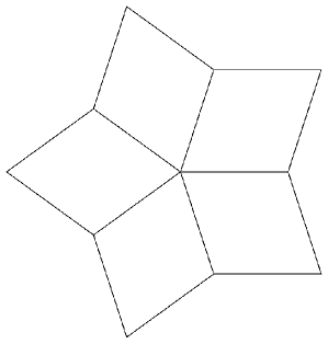
Figure 1: Two-dimensional star-shaped domain $\mathcal{S}_{I}$ whose center $\mathcal{V}_{I}$ is a vertex point where five regions $\mathcal{B}_{A}$ intersect.

A smooth reference metric is constructed on each star-shaped domain ${\cal S}_{I}$ by introducing local Cartesian coordinates on it that have smooth transition maps with the global multicube coordinates of each region ${\cal B}_{A}$ that it contains. Let $e^{I}_{ij}$ denote the flat Euclidean metric within ${\cal S}_{I}$, i.e., the tensor whose components are the unit matrix when written in terms of the local Cartesian coordinates of ${\cal S}_{I}$. These metrics are manifestly free of singularities within each $\mathcal{S}_{I}$, and they can be transformed from the local star-shaped domain coordinates into the global multicube coordinates in each $\mathcal{B}_{A}$ using the smooth transition maps that relate them.

These smooth metrics on the star-shaped domains $\mathcal{S}_{I}$ can be combined to form a global metric on $\Sigma$ by introducing a partition of unity $u_{I}({\vec{x}})$. These functions must be positive, $u_{I}({\vec{x}})>0$, for points ${\vec{x}}$ in the interior of ${\cal S}_{I}$; they must vanish, $u_{I}({\vec{x}})=0$, for points outside ${\cal S}_{I}$; and they are normalized so that $1=\sum_{I}u_{I}(\vec{x})$ at every point $\vec{x}$ in $\Sigma$. Using these functions, the tensor $\bar{g}_{ij}({\vec{x}})=\sum_{I}u_{I}({\vec{x}})\,e^{I}_{ij}({\vec{x}})$ is positive definite at each point ${\vec{x}}$ in $\Sigma$ and can therefore be used as a reference metric for $\Sigma$. Although each metric $e^{I}_{ij}$ is smooth within its own domain $\mathcal{S}_{I}$, it may not be smooth with respect to the Cartesian coordinates of the other star-shaped domains that intersect $\mathcal{S}_{I}$. For this reason the combined metric $\bar{g}_{ij}$ will generally only be as smooth as the products $u_{I}(\vec{x})\,e^{I}_{ij}$.

At the present time we only know how to construct functions $u_{I}(\vec{x})$ that make the combined metric $\bar{g}_{ij}$ continuous (but not $C^{1}$) across all the interface boundaries. The metric $\bar{g}_{ij}$ can be modified in a systematic and fairly straightforward way, however, to produce a new metric $\tilde{g}_{ij}$ whose extrinsic curvature $\tilde{K}_{ij}$ vanishes along each multicube interface boundary $\partial_{\alpha}\mathcal{B}_{A}$. Continuity of the extrinsic curvature is the geometrical condition needed to ensure the continuity of the derivatives of the metric across interface boundaries. The modified metrics $\tilde{g}_{ij}$ constructed in this way can therefore be used as $C^{1}$ reference metrics. In the two-dimensional case, the modification that converts $\bar{g}_{ij}$ into $\tilde{g}_{ij}$ can be accomplished using a simple conformal transformation. In higher dimensions, a more complicated transformation is required.

The following sections present detailed descriptions of our procedure for constructing reference metrics $\tilde{g}_{ij}$ on two-dimensional multicube manifolds having arbitrary topologies. In Sec. 2.1 an explicit method is described for systematically constructing the overlapping star-shaped domains ${\cal S}_{I}$; formulas are given for transforming between the intrinsic Cartesian coordinates in each ${\cal S}_{I}$ and the global Cartesian coordinates in ${\cal B}_{A}$; explicit representations are given (in both local and global Cartesian coordinates) for the flat metrics $e^{I}_{ij}(\vec{x})$ in each domain ${\cal S}_{I}$; and examples of useful $C^{0}$ partition of unity functions $u_{I}(\vec{x})$ are given. The resulting $C^{0}$ metrics are then modified in Sec. 2.2 by constructing an explicit conformal transformation that produces a metric having vanishing extrinsic curvature at each of the interface boundaries $\partial_{\alpha}\mathcal{B}_{A}$. The resulting metric is $C^{1}$ and can therefore be used as a reference metric for these manifolds.

We test these procedures for constructing reference metrics on a collection of compact, orientable two-dimensional manifolds in Sec. 2.3. New multicube representations of orientable two-dimensional manifolds having arbitrary topologies are described in detail in B. These procedures have been implemented in the Spectral Einstein Code (SpEC, developed by the SXS Collaboration, originally at Caltech and Cornell [21, 22, 23]). Reference metrics are constructed numerically in Sec. 2.3 for two-dimensional multicube manifolds with genera $N_{g}$ between zero and five; the scalar curvatures $\tilde{R}$ associated with these reference metrics are illustrated; and numerical results are presented which demonstrate that these two-dimensional reference metrics satisfy the Gauss-Bonnet identity up to truncation level errors (which converge to zero as the numerical resolution is increased). We also show that the continuous (but not $C^{1}$) reference metrics $\bar{g}_{ij}$ fail to satisfy the Gauss-Bonnet identity numerically because of the curvature singularities which occur on the interface boundaries in this case.

The scalar curvatures associated with the $C^{1}$ reference metrics constructed in Sec. 2 turn out to be quite nonuniform. Section 3 explores the possibility of using Ricci flow to smooth out the inhomogenities in these metrics $\tilde{g}_{ij}$. In particular we develop a slightly modified version of volume-normalized Ricci flow with DeTurck gauge fixing. This version is found to perform better numerically with regard to keeping the volume of the manifold fixed at a prescribed value. We describe our implementation of these new Ricci flow equations in SpEC in Sec. 3.1. We test this implementation by evolving a round-sphere metric with random perturbations on a six-region multicube representation of the two-sphere manifold, $S^{2}$. These tests show that our numerical Ricci flow works as expected: the solutions evolve toward constant-curvature metrics, the volumes of the manifolds are driven toward the prescribed values, and the Gauss-Bonnet identities remain satisfied throughout the evolutions. In Sec. 3.2 we use Ricci flow to evolve the rather nonuniform $C^{1}$ reference metrics $\tilde{g}_{ij}$ constructed in Sec. 2, using these $\tilde{g}_{ij}$ both as initial data and as the fixed reference metrics throughout the evolutions. We show that all these evolutions approach constant curvature metrics, as expected for two-dimensional Ricci flow. The volumes of these manifolds remain fixed throughout the evolutions, and the Gauss-Bonnet identities are satisfied for all the geometries tested (which include genera $N_{g}$ between zero and five). These Ricci-flow-evolved metrics therefore provide smoother and more uniform reference metrics for these manifolds.

2 Two-Dimensional Reference Metrics

This section develops a procedure for constructing reference metrics on multicube representations of two-dimensional manifolds. Continuous reference metrics are created in Sec. 2.1 and then transformed in Sec. 2.2 into metrics whose derivatives are also continuous across the multicube interface boundaries. The resulting $C^{1}$ reference metrics are tested in Sec. 2.3 (on two-dimensional manifolds with genera $N_{g}$ between zero and five) to ensure that they satisfy the appropriate Gauss-Bonnet identities.

2.1 Constructing Continuous Reference Metrics

The procedure for creating a continuous ($C^{0}$) reference metric $\bar{g}_{ij}$ presented here has three basic steps. First, a set of star-shaped domains ${\cal S}_{I}$ for the multicube manifold is constructed from a knowledge of the regions ${\cal B}_{A}$ and their interface boundary identification maps $\partial_{\alpha}{\cal B}_{A}=\Psi^{A\alpha}_{B\beta}(\partial_{\beta}{\cal B}_{B})$. The interiors of these ${\cal S}_{I}$ have the topology of open balls in $\mathbb{R}^{n}$ and together they form an open cover of the manifold $\Sigma$. The primary task in this first step of the procedure is to organize the multicube structure in a way that allows us to determine which star-shaped domain ${\cal S}_{I}$ is centered around each vertex $\nu_{A\mu}$ of each multicube region ${\cal B}_{A}$, and to determine how many regions ${\cal B}_{A}$ belong to each ${\cal S}_{I}$. In the second step, intrinsic Cartesian coordinates and metrics are constructed for each ${\cal S}_{I}$. These intrinsic coordinates are chosen to have smooth transformations with the global Cartesian coordinates in each multicube region ${\cal B}_{A}$. Metrics $e^{I}_{ij}$ for each star-shaped domain are introduced in this step to be the Euclidean metric expressed in terms of the intrinsic Cartesian coordinates in each ${\cal S}_{I}$. In the third step, partitions of unity $u_{I}({\vec{x}})$ are constructed that are positive for points $\vec{x}$ inside ${\cal S}_{I}$, that vanish for points $\vec{x}$ outside ${\cal S}_{I}$, and that sum to unity at each point in the manifold: $1=\sum_{I}u_{I}(\vec{x})$. A global reference metric is then obtained by taking weighted linear combinations of the flat metrics from each of the domains ${\cal S}_{I}$: $\bar{g}_{ij}({\vec{x}})=\sum_{I}u_{I}({\vec{x}})\,e^{I}_{ij}({\vec{x}})$. At present we only know how to choose the partition of unity functions $u_{I}(\vec{x})$ in a way that makes $\bar{g}_{ij}$ continuous across the boundary interfaces.

2.1.1 Step One

The first step is to compose and sort a list of all the vertices ${\nu}_{A\mu}$ in a given multicube structure. The index $\mu={\{1,...,2^{n}\}}$, where $n$ is the dimension of the manifold, identifies the vertices of a particular multicube region ${\cal B}_{A}$. This list of vertices $\nu_{A\mu}$ can be sorted into equivalence classes $\mathcal{V}_{I}$ whose members are identified with one another by the interface boundary-identification maps, i.e., $\nu_{A\mu}$ and $\nu_{B\sigma}$ belong to the same $\mathcal{V}_{I}$ iff there exists a sequence of maps $\Psi^{A\alpha}_{A_{1}\alpha_{1}}$,$\Psi^{A_{1}\alpha_{1}}_{A_{2}\alpha_{2}}$, …, $\Psi^{A_{n}\alpha_{n}}_{B\beta}$ with ${\nu}_{A\mu}=\left(\Psi^{A\alpha}_{A_{1}\alpha_{1}}\circ\Psi^{A_{1}\alpha_{1}}_{A_{2}\alpha_{2}}\circ\ldots\circ\Psi^{A_{n}\alpha_{n}}_{B\beta}\right)(\nu_{B\sigma})$.

One star-shaped domain ${\cal S}_{I}$ is centered on each equivalence class of vertices $\mathcal{V}_{I}$. The domain $\mathcal{S}_{I}$ consists of copies of all the multicube regions $\mathcal{B}_{A}$ having vertices that belong to the equivalence class $\mathcal{V}_{I}$. For two-dimensional manifolds, the primary computational task to be completed in this first step is to determine the number $K_{I}$ of vertices $\nu_{A\mu}$ that belong to each of the $\mathcal{V}_{I}$ classes. The quantity $K_{I}$ represents the number of multicube regions $\mathcal{B}_{A}$ clustered around the vertex $\mathcal{V}_{I}$ in the star-shaped domain $\mathcal{S}_{I}$. Our code performs this counting process in two dimensions by using the fact that each vertex $\nu_{A\mu}$ belongs to two different boundaries of the region ${\cal B}_{A}$. The code arbitrarily picks one of these boundaries, say $\partial_{\alpha}{\cal B}_{A}$, and follows the identification map $\Psi^{B\beta}_{A\alpha}$ to the neighboring region ${\cal B}_{B}$. The mapped vertex $\nu_{B\sigma}=\Psi^{B\beta}_{A\alpha}(\nu_{A\mu})$ again belongs to two boundaries of the new region ${\cal B}_{B}$: the mapped boundary $\partial_{\beta}{\cal B}_{B}$ and another one, say $\partial_{\gamma}{\cal B}_{B}$. The code then follows the map $\Psi^{C\delta}_{B\gamma}$ across this other boundary to its neighboring region ${\cal B}_{C}$ and to the new mapped vertex $\nu_{C\rho}=\Psi^{C\delta}_{B\gamma}(\nu_{B\sigma})$. Continuing in this way, the code makes a sequence of transitions between regions until it arrives back at the original vertex $\nu_{A\mu}$ of the starting region ${\cal B}_{A}$. The code counts these transitions and returns the number $K_{I}$ when the loop is closed. Figure 1 illustrates a two-dimensional star-shaped domain with $K_{I}=5$.

2.1.2 Step Two

The second step in this procedure is to construct local Cartesian coordinates that cover each of the star-shaped domains $\mathcal{S}_{I}$. We do this by noting that each $\mathcal{S}_{I}$ consists of a cluster of cubes $\mathcal{B}_{A}$ whose vertices coincide with the central point $\mathcal{V}_{I}$. If these cubes are appropriately distorted into parallelograms (by adjusting the angles between their coordinate axes), they can be fitted together (without overlapping and without leaving gaps between them) to form a domain in $\mathbb{R}^{n}$ whose interior has the topology of an open ball. Each $\mathcal{S}_{I}$ can therefore be covered by a single coordinate chart, which in two-dimensions can be written in the form $\bar{x}^{i}_{I}=(\bar{x}_{I},\bar{y}_{I})$. Figure 2 illustrates both the distorted (on the left) and the undistorted (on the right) representations of a two-dimensional $\mathcal{B}_{A}$.

Figure 2: Distorted and undistorted representations of a multicube region. Left side shows one of the two-dimensional multicube regions ${\cal B}_{A}$ that has been distorted to allow it to fit together with the other regions in a particular star-shaped domain $\mathcal{S}_{I}$. The vectors $\vec{\rho}_{\mu}$ and $\vec{\sigma}_{\mu}$ are tangent to the boundaries of ${\cal B}_{A}$. Right side is a representation of this same ${\cal B}_{A}$, showing the associations of the vectors $\vec{\rho}_{\mu}$ and $\vec{\sigma}_{\mu}$ for its various possible vertices (labeled by the index $\mu$).

In two dimensions the distortions needed to allow the $\mathcal{B}_{A}$ to be fitted around a vertex point $\mathcal{V}_{I}$ are quite simple: adjust the opening angles $\theta_{IA\mu}$ of the coordinate axes of each cube so they sum to $2\pi$ around each vertex, $\sum_{A\mu}\theta_{IA\mu}=2\pi$. The optimal way to satisfy this local flatness condition is to distort all of the two-dimensional cubes that make up $\mathcal{S}_{I}$ in the same way, i.e., by setting $\theta_{IA\mu}=2\pi/K_{I}$. In higher dimensions the problem of fitting the $\mathcal{B}_{A}$ together to form a smooth star-shaped domain (without conical singularites and without gaps) is more complicated. The complication in higher dimensions comes from the lack of uniqueness and a clear optimal choice, rather than being a fundamental problem of existence. We plan to study the problem of finding a practical way to perform this construction in higher dimensions in a future paper.

The simplest metric $\bar{e}^{I}_{ij}$ to assign to the star-shaped domain ${\cal S}_{I}$ is the flat Euclidean metric expressed in terms of the local coordinates of $\mathcal{S}_{I}$:

$$ds^{2}=\bar{e}^{I}_{ij}d\bar{x}^{i}_{I}d\bar{x}^{j}_{I}=d\bar{x}^{2}_{I}+d\bar{y}^{2}_{I}.$$ (1)

Each ${\cal B}_{A}$ that intersects ${\cal S}_{I}$ will inherit this flat geometry via the coordinate transformation that connects them. This fact can be used to deduce the coordinate transformations between the local Cartesian coordinates $\bar{x}^{i}_{I}=(\bar{x}_{I},\bar{y}_{I})$ of $\mathcal{S}_{I}$ and the global coordinates $x^{i}_{A}=(x_{A},y_{A})$ of $\mathcal{B}_{A}$. The left side of Fig. 2 shows a region ${\cal B}_{A}$ in $\mathcal{S}_{I}$ that has been distorted into a parallelogram having an opening angle $\theta_{IA\mu}$. The vectors $\vec{\rho}_{\mu}$ and $\vec{\sigma}_{\mu}$ in this figure represent unit vectors (according to the local flat metric of ${\cal S}_{I}$) that are tangent to the boundary faces of ${\cal B}_{A}$ at this vertex. The index $\mu$ identifies which of the vertices of ${\cal B}_{A}$ these unit vectors belong to. Since the opening angle at this particular vertex is $\theta_{IA\mu}$, the inner product of these vectors is just $\vec{\rho}_{\mu}\cdot\vec{\sigma}_{\mu}=\cos\theta_{IA\mu}$. The vectors $\vec{\rho}_{\mu}$ and $\vec{\sigma}_{\mu}$ are proportional to the coordinate vectors $\partial_{x}$ and $\partial_{y}$ of the global Cartesian coordinates used to describe points in the multicube region ${\cal B}_{A}$—exactly which coordinate vectors depends on which vertex of ${\cal B}_{A}$ coincides with this point. The right side of Fig. 2 shows these vectors at each of the vertices of ${\cal B}_{A}$, any of which could be the one that coincides with the center of ${\cal S}_{I}$. Table 1 gives the relationships between $\vec{\rho}_{\mu}$ and $\vec{\sigma}_{\mu}$ and the coordinate basis vectors in ${\cal B}_{A}$ for each vertex $\nu_{\mu}$. Also listed in Table 1 are the vectors $\vec{v}_{\mu}$ that give the location of each vertex relative to the center of its region ${\cal B}_{A}$.

Table 1: The vectors $\vec{\rho}_{\mu}$ and $\vec{\sigma}_{\mu}$ are proportional to the basis vectors $\vec{\partial}_{x}$ and $\vec{\partial}_{y}$ at each vertex $\mu$ of the region $\mathcal{B}_{A}$. This table gives the global Cartesian coordinate representations of $\vec{\rho}_{\mu}$ and $\vec{\sigma}_{\mu}$ at each vertex, the vertex-dependent constants $\epsilon_{\mu}$, and the locations $\vec{\nu}_{\mu}$ of the vertices with respect to the center of ${\cal B}_{A}$.

$\mu$	$\vec{\rho}_{\mu}$	$\vec{\sigma}_{\mu}$	$\epsilon_{\mu}$	$\vec{v}_{\mu}$
1	$(0,1)$	$(1,0)$	$+1$	$\frac{1}{2}L(-1,-1)$
2	$(1,0)$	$(0,-1)$	$-1$	$\frac{1}{2}L(-1,+1)$
3	$(0,-1)$	$(-1,0)$	$+1$	$\frac{1}{2}L(+1,+1)$
4	$(-1,0)$	$(0,1)$	$-1$	$\frac{1}{2}L(+1,-1)$

The inner products $\vec{\rho}_{\mu}\cdot\vec{\rho}_{\mu}$, $\vec{\sigma}_{\mu}\cdot\vec{\sigma}_{\mu}$, and $\vec{\rho}_{\mu}\cdot\vec{\sigma}_{\mu}$ are scalars that are independent of the coordinate representation of the vectors. Since $\vec{\rho}_{\mu}$ and $\vec{\sigma}_{\mu}$ are unit vectors that are (up to signs) just the coordinate basis vectors in the global Cartesian coordinates, it follows that the components of the metric $e^{I}_{ij}$ in the global coordinates of $\mathcal{B}_{A}$ must have the values $\vec{\rho}_{\mu}\cdot\vec{\rho}_{\mu}=\vec{\sigma}_{\mu}\cdot\vec{\sigma}_{\mu}=e^{I}_{xx}=e^{I}_{yy}=1$ and $\vec{\rho}_{\mu}\cdot\vec{\sigma}_{\mu}=\cos\theta_{IA\mu}=\epsilon_{\mu}\,e^{I}_{xy}$, where $\epsilon_{\mu}=\pm 1$ is the vertex-dependent constant defined in Table 1. The flat metric $e^{I}_{ij}$ of the region ${\cal S}_{I}\cap{\cal B}_{A}$ therefore has the form

$$ds^{2}=e^{IA}_{ij}dx^{i}_{A}dx^{j}_{A}=dx^{2}_{A}+2\epsilon_{\mu}\cos\theta_{IA\mu}\,dx_{A}\,dy_{A}+dy^{2}_{A}$$ (2)

when expressed in terms of the global Cartesian coordinates $x^{i}_{A}=(x_{A},y_{A})$ of ${\cal B}_{A}$. This metric can also be written as

$$ds^{2}=e^{IA}_{ij}dx^{i}_{A}dx^{j}_{A}=(dx_{A}+\epsilon_{\mu}\cos\theta_{IA\mu}\,dy_{A})^{2}+\sin^{2}\theta_{IA\mu}\,dy^{2}_{A}.$$ (3)

This is identical to the standard representation of $\bar{e}^{I}_{ij}$ in the local coordinates of ${\cal S}_{I}$, Eq. (1), if new coordinates $\tilde{x}_{IA}$ and $\tilde{y}_{IA}$ are defined as

$$\tilde{x}_{IA} = x_{A}-c^{x}_{A}-v^{x}_{\mu}+\epsilon_{\mu}\cos\theta_{IA\mu}\,(y_{A}-c^{y}_{A}-v^{y}_{\mu}),$$ (4)

$$\tilde{y}_{IA} = \sin\theta_{AI}\,(y-c^{y}_{A}-v^{y}_{\mu}).$$ (5)

The constants $c_{A}^{i}$ represent the global Cartesian coordinates of the center of region $\mathcal{B}_{A}$, and the constants $v_{\mu}^{i}$ represent the location of the $\mu$ vertex of the region relative to its center. These are included in the transformations in Eqs. (4) and (5) to ensure that the point $\tilde{x}_{IA}=\tilde{y}_{IA}=0$ corresponds to the point $\vec{x}=\vec{c}_{A}+\vec{v}_{\mu}$, which is the ${\nu}_{A\mu}$ vertex of ${\cal B}_{A}$ that coincides with the center of ${\cal S}_{I}$. These new coordinates $\tilde{x}_{IA}$ and $\tilde{y}_{IA}$ are therefore equal to the local Cartesian coordinates of ${\cal S}_{I}$, $\bar{x}_{I}$ and $\bar{y}_{I}$, up to a rigid rotation:

$$\bar{x}_{I} = \cos\psi_{IA}\,\tilde{x}_{IA}+\sin\psi_{IA}\,\tilde{y}_{IA},$$ (6)

$$\bar{y}_{I} = -\sin\psi_{IA}\,\tilde{x}_{IA}+\cos\psi_{IA}\,\tilde{y}_{IA},$$ (7)

for some angle $\psi_{IA}$. The composition of Eqs. (6) and (7) with Eqs. (4) and (5) therefore gives the transformation between the local Cartesian coordinates of ${\cal S}_{I}$, $\bar{x}_{I}$ and $\bar{y}_{I}$, and the global Cartesian coordinates, $x_{A}$ and $y_{A}$, of the multicube representation of the manifold.

The metric $e^{IA}_{ij}$ given in Eq. (2) must be constructed for each vertex $\nu_{A\mu}$ of each region ${\cal B}_{A}$ in terms of its global Cartesian coordinates $x_{A}^{i}$. These expressions depend only on the opening angles $\theta_{IA\mu}$, which in turn depend only on the parameter $K_{I}$. The full coordinate transformations between the global Cartesian coordinates $x_{A}$ and $y_{A}$ and the local coordinates $\bar{x}_{I}$ and $\bar{y}_{I}$ given in Eqs. (4)–(7) are not actually needed to evaluate the reference metrics.

2.1.3 Step Three

The third step in this procedure for constructing a reference metric is to build a partition of unity $u_{I}(\vec{x})$ that is adapted to the star-shaped domains. We do this by introducing a collection of weight functions $w_{I}(\vec{x})$ that are positive within a particular ${\cal S}_{I}$ and that fall to zero at its boundary. We experimented with a number of different weight functions and found that writing them as simple separable functions of the global Cartesian coordinates of each region $\mathcal{B}_{A}$ worked far better than anything else we tried. Thus we let

$$w_{I}(\vec{x})=h\left(\frac{x_{A}-c^{x}_{A}-v^{x}_{\mu}}{L}\right)h\left(\frac{y_{A}-c^{y}_{A}-v^{y}_{\mu}}{L}\right),$$ (8)

where $L$ is the coordinate size of each region $\mathcal{B}_{A}$. The functions $h(w)$ are chosen to have the value $h(0)=1$, which corresponds to the vertex point at the center of the domain $\mathcal{S}_{I}$, and the value $h(1)=0$ at the points which correspond to the outer boundary of $\mathcal{S}_{I}$. We find that the simple class of functions

$$h(w)=(1-w^{2k})^{\ell},$$ (9)

with integers $k>0$ and $\ell>0$, works quite well. Some of these functions are illustrated in Fig. 3, with integer values in the range that worked best in our numerical tests.

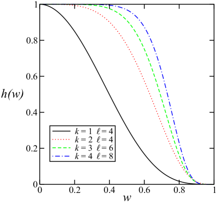
Figure 3: Weight functions $h(w)$ defined in Eq. (9) are positive for $0\leq w<1$ and vanish for $w=1$.

Figure 4 illustrates these weight functions expressed in terms of the local Cartesian coordinates of one of the star-shaped domains $\mathcal{S}_{I}$. This figure shows clearly that this choice of $u_{I}(\vec{x})$ is continuous but not $C^{1}$ across the interface boundaries. We could also make these functions $C^{1}$ with respect to the local coordinates in one of the $\mathcal{S}_{I}$, however it is not possible to make them $C^{1}$ with respect to all of the overlapping local star-shaped coordinates at the same time.

Figure 4: Weight function $w_{I}(\vec{x})$ illustrated on a star-shaped domain $\mathcal{S}_{I}$ where five regions $\mathcal{B}_{A}$ meet. Left illustration shows countours of $w_{I}(\vec{x})$, which uses the $h(w)$ functions defined in Eq. 9 with $k=1$ and $\ell=4$. Right illustration shows the same function in a three-dimensional rendering. This example illustrates the fact that these $w_{I}(\vec{x})$ are continuous but not $C^{1}$ across the region interface boundaries.

A partition of unity $u_{I}(\vec{x})$ is constructed from the weight functions $w_{I}(\vec{x})$ by normalizing them:

$$u_{I}(\vec{x})=\frac{w_{I}(\vec{x})}{H(\vec{x})},$$ (10)

where $H(\vec{x})$ is defined by

$$H(\vec{x})=\sum_{I}w_{I}(\vec{x}).$$ (11)

This definition ensures that the $u_{I}(\vec{x})$ satisfy the normalization condition $\sum_{I}u_{I}(\vec{x})=1$ for every point $\vec{x}$ in the manifold.

A global reference metric is constructed by combining the metrics $e^{I}_{ij}$ associated with each of the star-shaped domains $\mathcal{S}_{I}$ and defined in Eq. (2), using the partition of unity defined in Eq. (10):

$$\bar{g}_{ij}({\vec{x}})=\sum_{I}u_{I}({\vec{x}})\,e^{I}_{ij}({\vec{x}}).$$ (12)

This metric is positive definite, and it is continuous across all of the multicube interface boundaries. It can therefore be used as a continuous reference metric.

In an effort to reduce the spatial variation of the metric defined in Eq. (12) and thus reduce the required numerical resolution, we add additional terms of the form $u_{A}(\vec{x})\,e^{A}_{ij}$, where $e^{A}_{ij}$ are flat metrics with support in a single multicube region $\mathcal{B}_{A}$. Thus we let

$$ds^{2}=e^{A}_{ij}dx^{i}_{A}dx^{j}_{A}=dx^{2}_{A}+dy^{2}_{A}$$ (13)

be the flat Euclidean metric expressed in terms of the global Cartesian coordinates $x_{A}$ and $y_{A}$. We define new weight functions $w_{A}(\vec{x})$ associated with the individual multicube regions to be

$$w_{A}(\vec{x})=h\left(\frac{2(x_{A}-c^{x}_{A})}{L}\right)h\left(\frac{2(y_{A}-c^{y}_{A})}{L}\right),$$ (14)

which have the value $w_{A}(\vec{c}_{A})=1$ at the center of the region $\mathcal{B}_{A}$ and the value $w_{A}(\vec{x})=0$ for points $\vec{x}$ on its boundary. These weight functions can be combined with those assocated with the star-shaped domains, Eq. (8), to form a new partition of unity. We modify the normalization function $H(\vec{x})$ to be

$$H(\vec{x})=\sum_{I}w_{I}(\vec{x})+\sum_{A}w_{A}(\vec{x}).$$ (15)

Then we redefine the functions $u_{I}(\vec{x})$ using Eq. (10) with this new $H(\vec{x})$, and we define functions $u_{A}(\vec{x})$ using Eqs. (14) and (15):

$$u_{A}(\vec{x})=\frac{w_{A}(\vec{x})}{H(\vec{x})}.$$ (16)

A new metric is then formed by combining these region-centered metrics with the star-shaped domain metrics constructed above:

$$\bar{g}_{ij}({\vec{x}})=\sum_{I}u_{I}({\vec{x}})\,e^{I}_{ij}({\vec{x}})+\sum_{A}u_{A}({\vec{x}})\,e^{A}_{ij}({\vec{x}}).$$ (17)

The addition of the region-centered metrics does not appear to have a significant impact on the required numerical resolution. Nevertheless, this is the two-dimensional reference metric that we use (after conformally transforming as described in the following section) in the numerical work described in the later sections of this paper.

2.2 Constructing $C^{1}$ Reference Metrics

The continuous metric $\bar{g}_{ij}$ has been constructed in a way that ensures the geometry has no conical singularities at the vertices of the multicube regions. However, $\bar{g}_{ij}$ is not in general $C^{1}$ across the interface boundaries; e.g., the partition of unity that we use is not $C^{1}$ there. The geometry defined by $\bar{g}_{ij}$ will therefore have curvature singularities along those interface boundaries. In order to remove these singularities, our next goal is to modify $\bar{g}_{ij}$ by making it $C^{1}$, while at the same time keeping it continuous, positive definite, and free of conical singularities. It should be possible, for example, to find a tensor $\psi_{ij}$ that vanishes at the interface boundaries, and whose normal derivatives are the negatives of those of $\bar{g}_{ij}$. In this case the new tensor $\tilde{g}_{ij}=\bar{g}_{ij}+\psi_{ij}$ and its first derivatives should be continuous at the boundaries. There is in fact a great deal of freedom available in choosing $\psi_{ij}$. In particular, it can be changed arbitrarily in the interior of a region so long as its boundary values and derivatives remain unchanged. The idea is to use this freedom to keep $\psi_{ij}$ small enough everywhere that $\tilde{g}_{ij}$ remains positive definite. We plan to find a practical way to do this for manifolds of arbitrary dimension in a future work. In this paper we focus on the two-dimensional case, where a simple conformal transformation is all that is needed to make the continuous metric $\bar{g}_{ij}$ $C^{1}$. We introduce the conformal factor $\psi_{A}$ for the metric in multicube region $\mathcal{B}_{A}$:

$$\tilde{g}^{A}_{ij}=\psi^{4}_{A}\,\bar{g}^{A}_{ij}.$$ (18)

The conformal factor $\psi_{A}$ is chosen to make the resulting metric $\tilde{g}^{A}_{ab}$ and its derivatives continuous across interface boundaries.

The extrinsic curvature $\bar{K}^{A\alpha}_{ij}$ of the $\partial_{\alpha}\mathcal{B}_{A}$ boundary of cubic region $\mathcal{B}_{A}$ is defined by

$$\bar{K}^{A\alpha}_{ij}=(\delta^{k}_{i}-\bar{n}_{A\alpha}^{k}\bar{n}_{A\alpha i})\bar{\nabla}_{k}\bar{n}_{A\alpha j},$$ (19)

where $\bar{n}_{A\alpha}^{i}$ is the unit normal to the boundary and $\bar{\nabla}_{k}$ is the covariant derivative associated with the metric $\bar{g}^{A}_{ij}$. In two dimensions this can be rewritten as

$$\bar{K}^{A\alpha}_{ij}=(\bar{g}^{A}_{ij}-\bar{n}_{A\alpha i}\bar{n}_{A\alpha j})\bar{K}_{A\alpha},$$ (20)

where $\bar{K}_{A\alpha}=\bar{\nabla}_{k}\bar{n}^{k}_{A\alpha}$ is the trace. Since the normal vector $\bar{n}^{i}_{A\alpha}$ depends only on the metric $\bar{g}_{ij}$, its divergence can be written explicitly in terms of derivatives of the metric:

$$\bar{K}_{A\alpha} = \bar{\nabla}_{k}\bar{n}_{A\alpha}^{k}=\tfrac{1}{2}\left[\bar{n}^{i}_{A\alpha}(\bar{g}^{jk}+\bar{n}^{j}_{A\alpha}\bar{n}^{k}_{A\alpha})-2\bar{g}^{ij}\bar{n}^{k}_{A\alpha}\right]\partial_{i}\bar{g}_{jk}.\qquad$$ (21)

Under the conformal transformation given in Eq. (18), the trace of the extrinsic curvature $K_{A\alpha}$ transforms as follows:

$$\tilde{K}_{A\alpha}=\psi^{-2}_{A}(\bar{K}_{A\alpha}+2\bar{n}^{a}_{A\alpha}\bar{\nabla}_{a}\log\psi_{A}).$$ (22)

The idea is to choose the conformal factor $\psi_{A}$ so that it has the value $\psi_{A}=1$ on each interface boundary $\partial_{\alpha}\mathcal{B}_{A}$, with a normal derivative on each boundary given by

$$\bar{n}^{a}_{A\alpha}\bar{\nabla}_{a}\log\psi_{A}=-\tfrac{1}{2}\bar{K}_{A\alpha}.$$ (23)

These boundary conditions ensure that the metric $\tilde{g}_{ij}$ continues to be continuous everywhere and free of cone singularities at the vertices of each cubic-block region, while also ensuring that the extrinsic curvature at each interface boundary is zero.

There is no unique conformal factor satisfying the boundary conditions $\psi_{A}=1$ and the normal-derivative condition given in Eq. (23). However, the following expression for $\psi_{A}$ does satisfy these conditions:

$$\log\psi_{A} = -f\left(\frac{x_{A}-c_{A}^{x}}{L}+\frac{1}{2}\right)\frac{L\,\bar{K}_{A-x}(y_{A})}{2\,\bar{n}^{x}_{A-x}(y_{A})}+f\left(\frac{1}{2}-\frac{x_{A}-c_{A}^{x}}{L}\right)\frac{L\,\bar{K}_{A+x}(y_{A})}{2\,\bar{n}^{x}_{A+x}(y_{A})}$$ (24)

$$-f\left(\frac{y_{A}-c_{A}^{y}}{L}+\frac{1}{2}\right)\frac{L\,\bar{K}_{A-y}(x_{A})}{2\,\bar{n}^{y}_{A-y}(x_{A})}+f\left(\frac{1}{2}-\frac{y_{A}-c_{A}^{y}}{L}\right)\frac{L\,\bar{K}_{A+y}(x_{A})}{2\,\bar{n}^{y}_{A+y}(x_{A})}.$$

The required properties of the function $f(w)$ are that it has the values $f(0)=f(1)=0$ and the derivatives $f^{\prime}(0)=1$ and $f^{\prime}(1)=0$. The simple choice $f(w)=w\,h(w)$ satisfies these conditions, with $h(w)$ given in Eq. (9). The expression for the conformal factor in Eq. (24) has the property that $\log\psi_{A}=0$ everywhere on the boundary of the cubic-block region, while its derivatives on the boundary satisfy Eq. (23). The values of the extrinsic curvatures $\bar{K}_{A\alpha}$ and the normal vectors $\bar{n}^{i}_{A\alpha}$ used in Eq. (24) are those associated with the continuous metric $\bar{g}_{ij}$ given in Eq. (17).

Continuity of the extrinsic curvature across interface boundaries is the necessary and sufficient condition for the metric to be $C^{1}$ and singularity-free at those interfaces (cf. the Israel junction conditions [24]). The metrics $\tilde{g}_{ij}$ defined in Eq. (18), with conformal factor $\psi_{A}$ given by Eq. (24), will be $C^{1}$ even across the multicube interface boundaries, since their extrinsic curvatures vanish and are continuous there. The reference metrics $\tilde{g}_{ij}$ can thus be used to define a $C^{1}$ differential structure, which defines the continuity of tensor fields and their derivatives. A shows that this differential structure is unique in the sense that it is the same as would be produced by any other $C^{1}$ reference metric expressed in the same global multicube coordinates.

2.3 Testing the Reference Metrics

We have implemented the method outlined in Secs. 2.1 and 2.2 for constructing a $C^{1}$ reference metric $\tilde{g}_{ij}$ in SpEC. This section describes some tests we have performed to verify that our code correctly constructs reference metrics according to these procedures. We begin by constructing multicube representations of compact, orientable two-dimensional manifolds having genera $N_{g}$ between zero and five. B gives detailed descriptions of these multicube representations and also shows explicitly how they can be generalized to compact, orientable two-dimensional manifolds of any genus $N_{g}$. These multicube representations consist of lists of the regions $\mathcal{B}_{A}$ and their specific locations in $\mathbb{R}^{n}$, together with a complete list of the specific interface boundary identification maps $\Psi^{A\alpha}_{B\beta}$ that define how the regions are to be connected together.

Any $C^{1}$ metric $g_{ij}$, including the reference metric $\tilde{g}_{ij}$ from Eq. (18), must satisfy the Gauss-Bonnet identity, which relates the scalar curvature $R$ to the topology of any compact, orientable two-dimensional Riemannian manifold:

$$V\,||R||=8\pi(1-N_{g}),$$ (25)

where $||R||$ is the spatially averaged scalar curvature,

$$||R||=\frac{\int R\sqrt{g}\,d^{\,2}x}{V},$$ (26)

$V$ is the volume,

$$V=\int\!\sqrt{g}\,d^{\,2}x,$$ (27)

and where $N_{g}$ is the genus of the manifold. The Gauss-Bonnet identity therefore provides a powerful test: The multicube manifold must have the correct genus or the identity will fail. And the metric must be $C^{1}$ across all the interface boundaries, or curvature singularities along those boundaries will cause the numerical integrals used in the the identity to fail.

We use the quantity ${\cal E}_{GB}$, defined by

$${\cal E}_{GB}=\frac{\left|V\,||R||-8\pi(1-N_{g})\right|}{8\pi(1+N_{g})},$$ (28)

to monitor how well the Gauss-Bonnet identity is satisfied numerically in our tests. Figure 5 shows the values of ${\cal E}_{GB}$ computed for each of the multicube manifolds described in B using the $C^{1}$ reference metric $\tilde{g}_{ij}$ defined in Eq. (18). Each curve in Fig. 5 represents ${\cal E}_{GB}$ for a particular multicube manifold as a function of the numerical resolution $N$ (the number of grid points along each dimension of each multicube region $\mathcal{B}_{A}$). The manifolds are identified in Fig. 5 by their genera $N_{g}$ and the numbers of regions $N_{R}$ used in their particular representations. These graphs show that the Gauss-Bonnet identity is satisfied by the reference metrics $\tilde{g}_{ij}$ with numerical errors that decrease exponentially as the numerical resolution $N$ is increased. The numerical errors arise both in the numerical derivatives used in the computation of the scalar curvature $R$ and in the numerical integrations used to evaluate $||R||$. A minimum error of $\mathcal{O}(10^{-9})$ is reached at a resolution of about $N=46$, which corresponds to the level of accumulated roundoff error in the calculation of ${\cal E}_{GB}$ at that resolution.

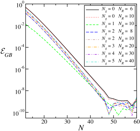
Figure 5: The error in the Gauss-Bonnet identity ${\cal E}_{GB}$, defined in Eq. (28), as a function of resolution for two-dimensional multicube manifolds having different genera $N_{g}$ and different numbers of multicube regions $N_{R}$.

We have also tested the Gauss-Bonnet identity on this same collection of multicube manifolds using the scalar curvatures computed from the continuous reference metrics $\bar{g}_{ij}$ of Eq. (17) instead of the $C^{1}$ metrics $\tilde{g}_{ij}$ of Eq. (18). Using these $C^{0}$ reference metrics, we find that $\mathcal{E}_{GB}$ is of order unity (with values between about 0.5 and 2) for all of the tests illustrated in Fig. 5. The Gauss-Bonnet identity fails in this case because the curvatures associated with the $C^{0}$ reference metrics have singularities along the multicube interface boundaries. This failure, which was expected in this case, reinforces the conclusion that we have successfully implemented the procedure outlined in Secs. 2.1 and 2.2 for constructing $C^{1}$ reference metrics on two-dimensional manifolds with arbitrary topologies.

3 Smoothing the Reference Metrics Using Ricci Flow

The $C^{1}$ reference metrics $\tilde{g}_{ij}$ introduced in Secs. 2.1 and 2.2 satisfy the minimal requirements needed to establish low-order differential structures on two-dimensional manifolds. These structures allow us to define the continuity of tensors and their derivatives, which is all that is required for solving the systems of second-order equations of most interest in mathematical physics. Unfortunately these metrics exhibit a great deal of spatial structure and consequently require fairly high numerical resolution to be represented accurately. Figure 6 illustrates the scalar curvature $\tilde{R}$ associated with these reference metrics $\tilde{g}_{ij}$ for the case of a six-region, $N_{R}=6$, representation of the genus $N_{g}=0$ multicube manifold (the two-sphere), and also for the case of a forty-region, $N_{R}=40$, representation of the genus $N_{g}=5$ multicube manifold (the five-handled sphere).

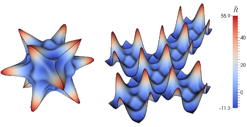
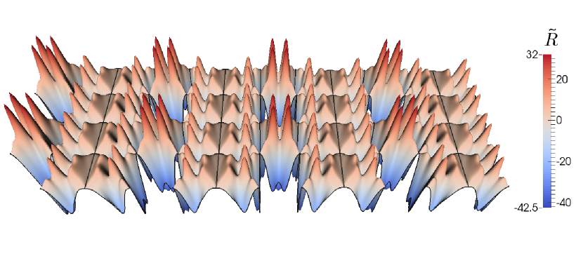
Figure 6: Illustration of the scalar curvature $\tilde{R}$ of two multicube manifolds with $C^{1}$ reference metrics $\tilde{g}_{ij}$ constructed via the procedure described in Sec. 2. Both cases use a numerical resolution of $N=40$ grid points along each dimension of each multicube region. Top: The genus $N_{g}=0$, six-region case. The left side shows the manifold mapped (non-isometrically) onto a 2-sphere, with radial warping proportional to the scalar curvature $\tilde{R}$. The right side shows the same manifold in the multicube Cartesian coordinates, with warping in the $z$-direction proportional to $\tilde{R}$. Bottom: The genus $N_{g}=5$, forty-region multicube manifold in the multicube Cartesian coordinates, with warping in the $z$-direction proportional to the scalar curvature $\tilde{R}$.

While these scalar curvatures appear to be continuous (even across the region interface boundaries) they have very large spatial variations. The goal of this section is to develop a method of transforming these metrics into more uniform (and smoother) reference metrics.

The uniformization theorem implies that every orientable two-dimensional manifold $\Sigma$ admits a metric having constant scalar curvature [25]. One approach to making the reference metrics $\tilde{g}_{ij}$ more uniform, therefore, would be to find a way to transform them into metrics having constant scalar curvatures. Fortunately there is a well-studied technique for doing exactly that. Volume-normalized Ricci flow is a parabolic evolution equation for the metric whose solutions in two dimensions all evolve toward metrics having spatially constant scalar curvatures [26, 27, 28, 25].

The evolution equation we use for the volume-normalized Ricci flow of a two-dimensional metric $g_{ij}$ is given by

$$\partial_{t}g_{ij} = -2R_{ij}+||R(t)||\,g_{ij}-\mu\frac{V(t)-V_{0}}{V(t)}\,g_{ij}+\nabla_{i}H_{j}+\nabla_{j}H_{i}.$$ (29)

The quantities $||R||$ and $V(t)$ in Eq. (29) are the volume-averaged scalar curvature and the volume of the manifold defined in Eqs. (26) and (27), respectively. The terms containing these quantities are added to control the volume of the manifold. The term proportional to $\mu$ in Eq. (29) is new to the best of our knowledge. We have found that it makes our numerical solutions of Eq. (29) track the target volume $V_{0}$ more accurately. The DeTurck gauge-fixing covector $H_{i}$ is defined by

$$H_{i}=g_{ij}g^{k\ell}(\Gamma^{j}_{k\ell}-\tilde{\Gamma}^{j}_{k\ell}),$$ (30)

where $\Gamma^{j}_{k\ell}$ is the connection associated with the metric $g_{ij}$, and $\tilde{\Gamma}^{j}_{k\ell}$ is any other fixed connection on the manifold [29]. The DeTurck terms (those containing $H_{i}$) are added to make Eq. (29) strongly parabolic, and thus to have a manifestly well-posed initial value problem [30].

Contracting Eq. (29) with the inverse metric $g^{ij}$ gives

$$\partial_{t}\log\sqrt{g}=-R+||R||-\mu\frac{V(t)-V_{0}}{V(t)}+\nabla_{i}H^{i}.$$ (31)

Integrating this equation over any compact manifold provides the evolution equation for the volume $V(t)$ of the manifold:

$$\partial_{t}\left[V(t)-V_{0}\right]=-\mu\left[V(t)-V_{0}\right].$$ (32)

Without the term proportional to $\mu$, the volume of the manifold would be fixed, $\partial_{t}V(t)=0$, at the analytical level. In numerical simulations, however, discretization and roundoff error give rise to slow, approximately linear drifts in the volume. With the damping term we have added, the volume of the manifold is driven toward the target value $V_{0}$ at a rate determined by the constant $\mu$. In our numerical tests, we find that a value of $\mu=10$ works well.

3.1 Numerical Ricci Flow

We have implemented the volume-normalized Ricci flow equation with DeTurck gauge fixing, Eq. (29), in SpEC. This code evolves PDEs using pseudo-spectral methods to evaluate spatial derivatives, and it performs explicit time integration at each collocation point using standard ordinary differential equation solvers (e.g., Runge-Kutta). Boundary conditions are imposed at multicube interface boundaries to enforce continuity of the metric $g_{ij}$ and its normal derivative $\tilde{n}^{k}\tilde{\nabla}_{k}g_{ij}$. The vector $\tilde{n}^{k}$ is the unit normal to the boundary and $\tilde{\nabla}_{k}$ is the covariant derivative associated with the reference metric $\tilde{g}_{ij}$.

Boundary conditions are imposed in SpEC using penalty methods. The desired boundary conditions are added to the evolution equations at the boundary collocation points. The evolution equations on the $\partial_{\alpha}\mathcal{B}_{A}$ boundary, which is identified with the $\partial_{\beta}\mathcal{B}_{B}$ boundary, for example, have the form

$$\partial_{t}g_{ij}=F_{ij}+\alpha\,\Bigl{(}g^{A}_{ij}-\langle g^{B}_{ij}\rangle_{A}\Bigr{)}+\beta\,\tilde{n}_{A}^{k}\Bigl{(}\tilde{\nabla}_{k}g^{A}_{ij}-\langle\tilde{\nabla}_{k}g^{B}_{ij}\rangle_{A}\Bigr{)},$$ (33)

where $F_{ij}$ represents the right side of Eq. (29), and $\alpha$ and $\beta$ are positive constant penalty factors. The quantities $\langle g^{B}_{ij}\rangle_{A}$ and $\langle\tilde{\nabla}_{k}g^{B}_{ij}\rangle_{A}$ represent the transformations of $g^{B}_{ij}$ and $\tilde{\nabla}_{k}g^{B}_{ij}$ into the tensor basis of region $\mathcal{B}_{A}$ using the interface boundary Jacobians:

$$\langle g^{B}_{ij}\rangle_{A} = J^{*B\beta a}_{A\alpha i}J^{*B\beta b}_{A\alpha j}g^{B}_{ab},$$ (34)

$$\langle\tilde{\nabla}_{k}g^{B}_{ij}\rangle_{A} = J^{*B\beta a}_{A\alpha i}J^{*B\beta b}_{A\alpha j}J^{*B\beta c}_{A\alpha k}\,\tilde{\nabla}_{c}g^{B}_{ab}.$$ (35)

If the penalty factors $\alpha$ and $\beta$ are chosen properly, these additional terms drive the evolution at the boundary in a way that reduces any small boundary condition error [31]. There is a range of constants $\alpha$ and $\beta$ that work well—too small can lead to instability, while too large may make the system overly stiff. Empirically, we have found that the following values work well in most cases:

$$\alpha=\tfrac{1}{2}N^{3}(N+1),\quad\beta=\tfrac{1}{2}N(N+1).$$ (36)

In some cases the penalty factors (particularly $\alpha$) can be decreased below the values given in Eq. (36) without sacrificing stability. Using smaller values allows a less restrictive condition on the size of the maximum time step and therefore allows more efficient numerical evolutions. In rare cases, we have found it necessary to increase $\beta$ above the value given in Eq. (36). For example, in the low-resolution $N=16$, ten-region, $N_{R}=10$, genus $N_{g}=0$ case, a value of $\beta$ at least twice that given in Eq. (36) was needed for stability. Hesthaven and Gottlieb [31] have derived rigorous lower bounds on the penalty factors needed for stable evolution of a simple, second-order parabolic equation in one dimension. They show that when Robin-type boundary conditions are used (like those we use here), penalty factors that scale like $\alpha\sim\mathcal{O}(N^{2})$ and $\beta\sim\mathcal{O}(N^{2})$ are required. Our results agree with theirs for $\beta$, but we have found it necessary to use much larger values of $\alpha$ that scale as $\alpha\sim\mathcal{O}(N^{4})$ in most cases.

We test the stability and robustness of our implementation of these Ricci flow evolution equations on a six-region, $N_{R}=6$, multicube representation of the two-sphere manifold, $S^{2}$, which is described in detail in B.1. As initial data for these tests we use the standard round-sphere metric with pseudo-random white noise of amplitude $0.1$ added to each component of the metric $g_{ij}$ at each collocation point. The reference metric $\tilde{g}_{ij}$ used in these tests is the usual smooth, unperturbed round-sphere metric, which is given explicitly in global Cartesian multicube coordinates in Ref. [19].

We use several measures to determine whether our implementation of numerical Ricci flow is working properly and whether it actually drives the metric toward a constant-curvature state, as it is expected to do in two dimensions. First, we measure how well the numerical Ricci flow evolves toward geometries having uniform scalar curvatures. One possible dimensionless measure of this scalar-curvature uniformity is the quantity $\tilde{\cal E}_{R}$, defined by

$$\tilde{\cal E}_{R}^{2}=\frac{\int(R-||R||)^{2}\sqrt{g}\,d^{\,2}x}{V||R||^{2}}.$$ (37)

For the two-dimensional manifolds studied here, the volume-averaged scalar curvature $||R||$ is given by the Gauss-Bonnet identity: $||R||=8\pi(1-N_{g})/V$. The scalar-curvature uniformity measure can therefore be rewritten in the form

$$\tilde{\cal E}_{R}^{2}=\frac{V\int(R-||R||)^{2}\sqrt{g}\,d^{\,2}x}{[8\pi(1-N_{g})]^{2}}.$$ (38)

This measure is singular for $N_{g}=1$, so we define an alternative measure ${\cal E}_{R}$ as follows:

$${\cal E}_{R}^{2}=\frac{V\int(R-||R||)^{2}\sqrt{g}\,d^{\,2}x}{[8\pi(1+N_{g})]^{2}}.$$ (39)

This alternative measure is well defined for all compact, orientable two-dimensional manifolds. It differs from $\tilde{\cal E}_{R}$ by the factor $|1-N_{g}|/(1+N_{g})$, which is of order unity, except for the singular case $N_{g}=1$. We use the measure ${\cal E}_{R}$ to monitor the uniformity of the scalar curvature in all of our Ricci flow evolutions. Second, we monitor the volume of the manifold to determine whether the volume-normalized flow is working properly. We do this using the dimensionless quantity ${\cal E}_{V}$, defined by

$${\cal E}_{V}=\frac{|V(t)-V_{0}|}{V_{0}},$$ (40)

to measure the fractional change in the volume relative to the target volume $V_{0}$. Third, we use the quantity ${\cal E}_{H}$ to measure the evolution of the DeTurck gauge-source covector:

$${\cal E}_{H}^{2}=\frac{\int g^{ij}H_{i}H_{j}\sqrt{g}\,d^{\,2}x}{\int\sum_{ij}\left(|g_{ij}|^{2}+\sum_{k}|\partial_{k}g_{ij}|^{2}\right)\sqrt{g}\,d^{\,2}x}.$$ (41)

And finally, we assess how well the geometries produced by this Ricci flow satisfy the Gauss-Bonnet identity, using the quantity $\mathcal{E}_{GB}$ defined in Eq. (28).

Figure 7 shows the results of our Ricci flow evolutions using initial data constructed from the round-sphere metric with random noise perturbations. This figure plots the time evolutions of the four error measures $\mathcal{E}_{R}$, $\mathcal{E}_{V}$, $\mathcal{E}_{H}$, and $\mathcal{E}_{GB}$, defined in Eqs. (39), (40), (41), and (28), respectively, for evolutions performed with several different numerical resolutions $N$. As evidenced in these figures, the Ricci flow evolutions are stable and convergent as the numerical resolution $N$ is increased. Nonuniformities in the random initial scalar curvature, as measured by ${\cal E}_{R}$ and shown in the upper left part of Fig. 7, decay exponentially in time as the geometry evolves toward the constant-curvature round-sphere metric until the differences are dominated by truncation level errors at each resolution. The upper right part of Fig. 7 shows that the volume-controlling terms in Eq. (29) are effective at driving the volume of the manifold to the value $V_{0}$, as measured by $\mathcal{E}_{V}$. The target volume $V_{0}$ in these tests was taken to be the volume measured by the smooth round-sphere reference metric, rather than the volume of the initial random metric. The lower left part of Fig. 7 shows that the gauge source one-form $H_{i}$, measured by ${\cal E}_{H}$, is effectively driven to zero by the DeTurck term, and the lower right part of Fig. 7 shows that the Gauss-Bonnet error ${\cal E}_{GB}$ decays very quickly to truncation level at each resolution. Random noise was added to the initial data in these tests at each grid point, so the precise structure of the initial data is different at each resolution. Therefore, numerical convergence with increasing resolution $N$ at the initial and very early times was not expected (or observed).

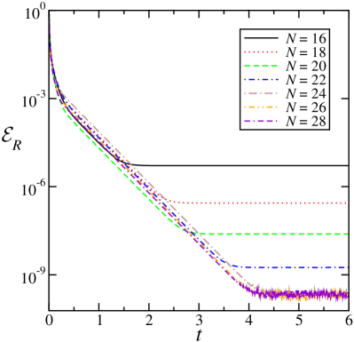
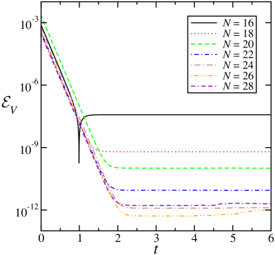
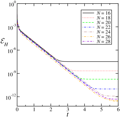
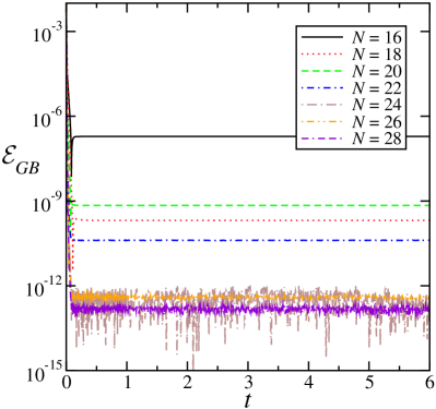
Figure 7: Ricci flow evolutions of a six-region, $N_{R}=6$, multicube representation of the 2-sphere, with random noise added to the round-sphere metric as the initial data. Graphs show the evolutions of the scalar-curvature uniformity measure $\mathcal{E}_{R}$, the volume-normalization error $\mathcal{E}_{V}$, the DeTurck gauge-covector norm $\mathcal{E}_{H}$, and the Gauss-Bonnet identity error $\mathcal{E}_{GB}$. These quantities are defined in Eqs. (39), (40), (41), and (28), respectively. The reference metric used in these tests is the usual unperturbed round-sphere metric. The numerical resolution in each spatial dimension of each square region is denoted by $N$.

3.2 Smoother Reference Metrics

We have used volume-normalized Ricci flow to construct smoother and more uniform reference metrics for several multicube manifolds in two dimensions. In particular we have performed Ricci-flow smoothing of the reference metrics for multicube representations of compact, orientable two-dimensional manifolds with genera between $N_{g}=0$ (the two-sphere) and $N_{g}=5$ (the five-handled two-sphere). In each case, initial data for the evolution are prepared by constructing the metric $\tilde{g}_{ij}$ according to the procedure described in Sec. 2. These $\tilde{g}_{ij}$ use the polynomial generating functions $h(w)$ of Eq. (9), with $k=1$ and $\ell=4$, both for the partition of unity and for the functions $f(w)=w\,h(w)$ that appear in the conformal factor in Eq. (24). Although this choice of powers appears to give the best results, we have found that other choices often work nearly as well. We use the metric $\tilde{g}_{ij}$ not only as initial data for these Ricci flow evolutions, but also as the fixed reference metric, which defines the continuity of all tensor fields and their derivatives throughout the evolutions, including the Ricci-flow-evolved $g_{ij}(t)$.

We have performed Ricci flow evolutions on all the multicube manifolds described in B, and the results look very similar to one another. For this reason we describe only one of these cases in detail, and then we summarize and compare the results of our highest-resolution evolutions from all of the cases. We show detailed results for our most complex case: a forty-region, $N_{R}=40$, representation of a genus $N_{g}=5$ multicube manifold (the five-handled two-sphere). The scalar curvature for the reference metric $\tilde{g}_{ij}$ in this case is illustrated in the bottom part of Fig. 6. The details of the multicube structure for this case (and all our other cases) are given in B.

Figure 8 shows the results of these genus $N_{g}=5$ evolutions for several different numerical resolutions $N$.

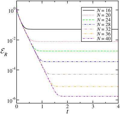
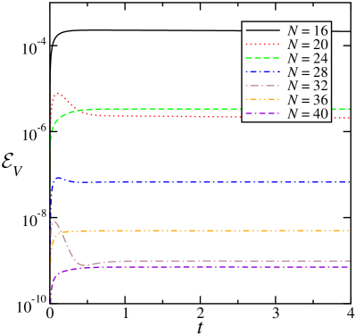
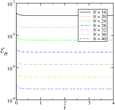
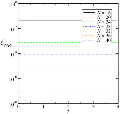
Figure 8: Ricci flow evolutions of a genus $N_{g}=5$, forty-region, $N_{R}=40$, multicube manifold. Graphs show the evolutions of the scalar-curvature uniformity measure $\mathcal{E}_{R}$, the volume-normalization error $\mathcal{E}_{V}$, the DeTurck gauge-covector norm $\mathcal{E}_{H}$, and the Gauss-Bonnet identity error $\mathcal{E}_{GB}$. These quantities are defined in Eqs. (39), (40), (41), and (28), respectively. The reference metric, which is identical to the initial metric in this case, is constructed according to the procedure described in Sec. 2. The numerical resolution in each spatial dimension of each multicube region is denoted by $N$.

The graphs in Fig. 8 indicate that the evolutions are stable and convergent, demonstrating our ability to evolve PDEs on arbitrary, complicated two-dimensional manifolds using the $C^{1}$ reference metrics developed in Sec. 2. These evolutions differ from the random-metric evolutions shown in Fig. 7 in several ways. First, these initial data are much smoother than the random metrics (which are unresolved by construction). Consequently, the Gauss-Bonnet error $\mathcal{E}_{GB}$ is much smaller at early times. Second, the initial metric in these tests is identical to the reference metric, and accordingly the error measures $\mathcal{E}_{V}$ and $\mathcal{E}_{H}$ are much smaller (about truncation level) at early times. These error measures remain close to these initial truncation-error levels throughout the evolutions. We also note that the more complicated spatial structures of the reference metrics in these simulations require somewhat higher numerical resolutions in order to obtain the same level of truncation errors as the random-metric $S^{2}$ tests described in Sec. 3.1.

Figure 9 compares the highest-resolution Ricci flow evolutions from each of the multicube manifolds described in B (up to and including the forty-region representation of a genus 5 manifold).

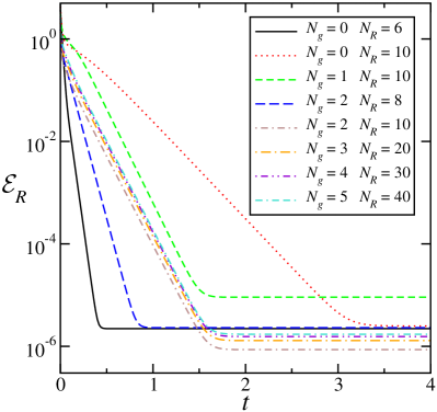
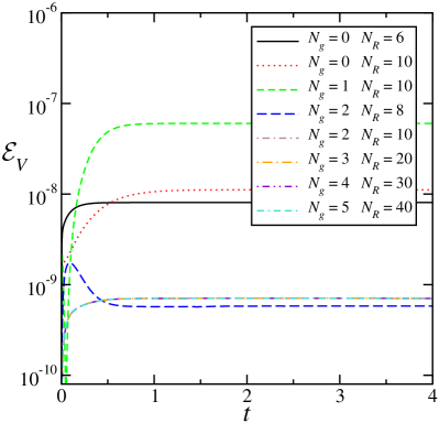
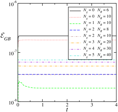
Figure 9: High-resolution ($N=40$) results of Ricci flow evolutions on a variety of different multicube manifolds. The genus $N_{g}$ and the number of multicube regions $N_{R}$ of each case are indicated in the legends. Graphs show the evolutions of the scalar-curvature uniformity measure $\mathcal{E}_{R}$, the volume-normalization error $\mathcal{E}_{V}$, the DeTurck gauge-covector norm $\mathcal{E}_{H}$, and the Gauss-Bonnet identity error $\mathcal{E}_{GB}$. These quantities are defined in Eqs. (39), (40), (41), and (28), respectively. In each case, the reference metric is identical to the initial metric and is constructed according to the procedure described in Sec. 2.

All of these cases are found to be stable and convergent, with qualitatively similar results to the genus $N_{g}=5$ evolutions shown in Fig. 8. The only significant difference between the cases is the rate at which nonuniformities in the scalar curvatures decay. The reference metrics that we construct on these different multicube manifolds have nonuniformities on different length scales, and these nonuniformities correspondingly decay at different rates under the Ricci flow. There are also differences in the levels of the truncation errors for these cases at the same numerical resolution. The ten-region, $N_{R}=10$, representation of the genus $N_{g}=1$ multicube manifold (the two-torus), for example, has the highest level of truncation error among the examples we have studied.

4 Discussion

This paper presents a method for constructing reference metrics on multicube representations of manifolds having arbitrary topologies. The method was implemented and successfully tested, as described in Sec. 2, for a variety of compact, orientable two-dimensional Riemannian manifolds with genera between $0$ and $5$. The reference metrics constructed in this way are not smooth, but they have continuous derivatives, which is sufficient to define the $C^{1}$ differential structures needed for solving the systems of second-order PDEs of most interest in mathematical physics. We have demonstrated in Sec. 3, for example, that these $C^{1}$ reference metrics can be used successfully to solve systems of second-order parabolic evolution equations.

The reference metrics constructed using the methods in Sec. 2 have large spatial variations, which are not easy to resolve numerically. We demonstrate in Sec. 3 that these metrics can be made more uniform by evolving them with Ricci flow. The two-dimensional reference metrics studied in our tests all evolve under Ricci flow to metrics having constant scalar curvatures.

Ricci flow also has smoothing properties similar to the heat equation: solutions to the Ricci flow equation on compact manifolds become smooth, in fact real-analytic, for $t>0$ provided the initial curvature is bounded (which is the case for our $C^{1}$ reference metrics) [32, 33]. Our numerical evolutions show smoothing of the metrics that is consistent with this fact. The presence of the DeTurck gauge-fixing terms, however, somewhat obfuscates this question of smoothness. Our evolutions show that the DeTurck gauge-fixing covector $H_{i}$ is zero, up to truncation level errors, throughout the evolutions. The connection $\Gamma^{k}_{ij}$ of the metric $g_{ij}$ at the end of our Ricci flow evolutions could (in principle) therefore retain some of the non-smooth features of the reference connection $\tilde{\Gamma}^{k}_{ij}$, since $H_{i}=0=g_{ij}g^{k\ell}(\Gamma^{j}_{k\ell}-\tilde{\Gamma}^{j}_{k\ell})$. However, the vanishing of $H_{i}$ shows that the evolved metric satisfies the original Ricci flow equation without the DeTurck terms, and thus must be smooth by the aforementioned theorems [32, 33]. Hence any non-smoothness of the connection must just reflect the (non-smooth) coordinate transitions at the interface boundaries.

We made some effort to avoid even the potential effects of the non-smoothness of the connection associated with the DeTurck terms by modifying the basic Ricci flow Eq. (29) in various ways. For example, we attempted to carry out numerical Ricci flow evolutions without including the DeTurck terms at all, i.e., simply by setting $H_{i}=0$ in Eq. (29). All of these evolutions were unstable. The DeTurck terms were added to the Ricci flow equation to make it strongly parabolic and thereby manifestly well-posed [25]. Without the DeTurck terms, the basic Ricci flow equations may simply be ill-suited for numerical solution. We also tried modifying the DeTurck terms in a way that would attempt to drive the solution to harmonic gauge, i.e., to a gauge in which $0=g^{ij}\Gamma^{k}_{ij}$. We did this by changing the definition of $H_{i}$ to give the reference connection an explicit time dependence, as in $H_{i}=g_{ij}g^{k\ell}(\Gamma^{j}_{k\ell}-e^{-\mu t}\,\tilde{\Gamma}^{j}_{k\ell})$, for example. Unfortunately all of these runs failed as well. While these runs appeared to be stable, the Ricci flows in these cases did not evolve toward metrics having constant scalar curvatures, and the DeTurck gauge-source covector $H_{i}$ did not remain small during the evolutions.

We plan to continue to search for effective and efficient ways to construct reference metrics on manifolds with arbitrary spatial topologies. In two dimensions the remaining questions are related to finding better gauge conditions for the reference metrics. In three and higher dimensions the challenge will be to find efficient ways to implement the general techniques developed here.

Appendix A Uniqueness of the $C^{1}$ Multicube Differential Structure

The traditional definition of a $C^{k}$ differential structure on a manifold consists of an atlas of coordinate charts having the property that the transition maps between overlapping charts are $C^{k+1}$ functions. Tensor fields are defined to be $C^{k}$ with respect to this differential structure if their components when represented in terms of this atlas are $C^{k}$ functions. In a multicube representation of a manifold, we define the continuity of tensor fields and their derivatives instead using the Jacobians and the connection determined by a reference metric. This enables us to define these concepts without needing an overlapping $C^{k+1}$ atlas. The two definitions of differential structure are equivalent on any manifold having both a multicube structure and a $C^{k+1}$ atlas. In this appendix we consider the technical question of the uniqueness of the multicube method of specifying the differential structure.

The purpose of this appendix is to show that the $C^{1}$ differential structure of a multicube manifold defined by a particular $C^{1}$ reference metric is independent of the choice of reference metric. In particular, we show that the definitions of continuity of tensor fields and their covariant derivatives based on a $C^{1}$ reference metric $\tilde{g}_{ab}$ are the same as those based on any other $C^{1}$ metric $\check{g}_{ab}$, i.e., any metric $\check{g}_{ab}$ that is continuous and whose covariant gradient $\tilde{\nabla}_{a}\check{g}_{bc}$ is continuous with respect to the differential structure defined by $\tilde{g}_{ab}$. Since any $C^{k}$ metric with $k\geq 1$ is also $C^{1}$, this argument implies that the $C^{1}$ differential structure defined by the $C^{1}$ metric $\tilde{g}_{ab}$ is also equivalent to the $C^{1}$ differential structure defined by any $C^{k}$ metric $\check{g}_{ab}$.

We have shown [19] how the differential structure for a multicube representation of a manifold may be specified by giving a $C^{1}$ metric $\tilde{g}_{ab}$ represented in the global Cartesian multicube coordinate basis. This method of defining the differential structure constructs Jacobians $\tilde{J}^{A\alpha a}_{B\beta b}$ and their duals $\tilde{J}_{A\alpha a}^{*B\beta b}$ that transform tensors from the $\partial_{\beta}\mathcal{B}_{B}$ face of cubic region $\mathcal{B}_{B}$ to the $\partial_{\alpha}\mathcal{B}_{A}$ face of cubic region $\mathcal{B}_{A}$. These Jacobians are determined by the metric $\tilde{g}_{ab}$ and the rotation matrices $C^{A\alpha a}_{B\beta b}$ that define the identification maps (cf. B) between neighboring regions. The expressions for these Jacobians are given by Lindblom and Szilágyi [19]:

$$\tilde{J}^{A\alpha a}_{B\beta b} = C^{A\alpha a}_{B\beta c}\left(\delta^{c}_{b}-\tilde{n}^{c}_{B\beta}\tilde{n}_{B\beta b}\right)-\tilde{n}^{a}_{A\alpha}\tilde{n}_{B\beta b},$$ (42)

$$\tilde{J}_{A\alpha a}^{*B\beta b} = \left(\delta^{c}_{a}-\tilde{n}_{A\alpha a}\tilde{n}^{c}_{A\alpha}\right)C^{B\beta b}_{A\alpha c}-\tilde{n}_{A\alpha a}\tilde{n}^{b}_{B\beta}.$$ (43)

The vectors $\tilde{n}^{a}_{A\alpha}$ and $\tilde{n}^{a}_{B\beta}$ that appear in these expressions represent the outward directed unit normal vectors to the $\partial_{\alpha}\mathcal{B}_{A}$ face of region $\mathcal{B}_{A}$ and the $\partial_{\beta}\mathcal{B}_{B}$ face of cubic region $\mathcal{B}_{B}$, respectively. These normals are unit vectors with respect to the $\tilde{g}_{ab}$ metric, i.e., $1=\tilde{g}_{Aab}\tilde{n}^{a}_{A\alpha}\tilde{n}^{b}_{A\alpha}=\tilde{g}_{Bab}\tilde{n}^{a}_{B\beta}\tilde{n}^{b}_{B\beta}$. These Jacobians, defined in Eqs. (42) and (43), determine the way continuous tensor fields transform across interface boundaries. The reference metric also determines a covariant derivative $\tilde{\nabla}_{a}$ that, together with the Jacobians, defines how $C^{1}$ tensor fields transform across interface boundaries. These definitions of continuity for tensor fields and their derivatives determine the $C^{1}$ differential structure of the manifold. The question of the uniqueness of the $C^{1}$ differential structure reduces therefore to the questions of the uniqueness of the Jacobians $\tilde{J}^{A\alpha a}_{B\beta b}$, and of the uniqueness of the continuity of the derivatives determined by the covariant derivative $\tilde{\nabla}_{a}$.

The normal covectors $\tilde{n}_{A\alpha a}$ that appear in Eqs. (42) and (43) are proportional to the gradients of the $x^{|\alpha|}_{A}$=constant coordinate surfaces that define the particular boundary face of the region (i.e., in this case the $\alpha$ face of region $A$):

$$\tilde{n}_{A\alpha a}=\tilde{N}_{A\alpha}\partial_{a}x^{|\alpha|}_{A}.$$ (44)

The index $\alpha$ can have either sign, e.g., to represent the $+x$ or the $-x$ coordinate boundary face. The notation $x^{|\alpha|}_{A}$ indicates the coordinate associated with either case—i.e., both the $+x$ and the $-x$ faces are surfaces of constant $x^{x}_{A}$. The proportionality constant $\tilde{N}_{A\alpha}$ in Eq. (44) is determined by the requirement that $\tilde{n}_{A\alpha a}$ is a unit covector with respect to the reference metric $\tilde{g}_{Aab}$:

$$\tilde{N}^{-2}_{A\alpha}=\tilde{g}^{ab}_{A}\partial_{a}x^{|\alpha|}_{A}\partial_{b}x^{|\alpha|}_{A}.$$ (45)

The sign of $\tilde{N}_{A\alpha}$ is chosen to ensure that $\tilde{n}_{A\alpha a}$ is the outward directed normal. The normal vector is defined as the dual to this normal covector: $\tilde{n}^{a}_{A\alpha}=\tilde{g}^{ab}_{A}\tilde{n}_{A\alpha b}$.

The Jacobians defined in Eqs. (42) and (43) transform these normals across interface boundaries in the appropriate way:

$$\tilde{n}^{a}_{A\alpha} = -\tilde{J}^{A\alpha a}_{B\beta b}\tilde{n}^{b}_{B\beta},$$ (46)

$$\tilde{n}_{A\alpha a} = -\tilde{J}_{A\alpha a}^{*B\beta b}\tilde{n}_{B\beta b}.$$ (47)

They also transform vectors $t^{a}_{B\beta}$ that are tangent to the interface, $\tilde{n}_{A\alpha a}t^{a}_{A\alpha}=0$, by the rotations $C^{A\alpha a}_{B\beta b}$ used to define the interface boundary maps (cf. B):

$$t^{a}_{A\alpha}=\tilde{J}^{A\alpha a}_{B\beta b}t^{b}_{B\beta}=C^{A\alpha a}_{B\beta b}t^{b}_{B\beta}.$$ (48)

These Jacobians and dual Jacobians are inverses of each other as well (cf. Ref. [19]):

$$\delta^{a}_{b}=\tilde{J}^{A\alpha a}_{B\beta c}\tilde{J}_{A\alpha b}^{*B\beta c}.$$ (49)

Now consider a second positive-definite metric $\check{g}_{ab}$ that is $C^{1}$ with respect to the differential structure defined by the metric $\tilde{g}_{ab}$. This second metric can be used to define alternate normal covectors $\check{n}_{A\alpha a}=\check{N}_{A\alpha}\partial_{a}x_{A}^{|\alpha|}$ and vectors $\check{n}^{a}_{A\alpha}=\check{g}^{ab}_{A}\check{n}_{A\alpha b}$, with $\check{N}_{A\alpha}^{-2}=\check{g}^{ab}_{A}\partial_{a}x^{|\alpha|}_{A}\partial_{b}x^{|\alpha|}_{A}$. It follows from Eq. (47) and the continuity of $\check{g}_{ab}$ that the norm of $\tilde{n}_{A\alpha a}$ with respect to $\check{g}_{ab}$ is continuous across interface boundaries:

$$\check{g}^{ab}_{A}\tilde{n}_{A\alpha a}\tilde{n}_{A\alpha b}=\check{g}^{ab}_{B}\tilde{n}_{B\beta a}\tilde{n}_{B\beta b}.$$ (50)

This norm can be rewritten as

$$\check{g}^{ab}_{A}\tilde{n}_{A\alpha a}\tilde{n}_{A\alpha b}=\tilde{N}_{A\alpha}^{2}\check{g}^{ab}_{A}\partial_{a}x^{|\alpha|}_{A}\partial_{b}x^{|\alpha|}_{A}=\left(\frac{\tilde{N}_{A\alpha}}{\check{N}_{A\alpha}}\right)^{2}\!\!\!.\quad$$ (51)

Equation (50) therefore implies the continuity of the ratio $\tilde{N}_{A\alpha}/\check{N}_{A\alpha}$ across interface boundaries. The alternate normal $\check{n}_{A\alpha a}$, which can be written as $\check{n}_{A\alpha a}=(\check{N}_{A\alpha}/\tilde{N}_{A\alpha})\tilde{n}_{A\alpha a}$, is therefore continuous (up to a sign flip) across interface boundaries. This also implies that the alternate normal vector $\check{n}^{a}_{A\alpha}=\check{g}^{ab}_{A}\check{n}_{A\alpha b}$ is continuous. These alternate normals must therefore satisfy the same continuity conditions (up to the sign flips) across interface boundaries as any continuous tensor field:

$$\check{n}^{a}_{A\alpha} = -\tilde{J}^{A\alpha a}_{B\beta b}\check{n}^{b}_{B\beta},$$ (52)

$$\check{n}_{A\alpha a} = -\tilde{J}_{A\alpha a}^{*B\beta b}\check{n}_{B\beta b}.$$ (53)

The normal vector $\tilde{n}^{a}_{A\alpha}$ together with a collection of linearly independent tangent vectors, i.e., vectors $t^{a}_{A\alpha(k)}$ satisfying $0=t^{a}_{A\alpha(k)}\tilde{n}_{A\alpha a}$, can be used as a basis of vector fields on the boundary. Therefore any vector field, including $\check{n}^{a}_{A\alpha}$, can be expressed as a linear combination of the form

$$\check{n}^{a}_{A\alpha}=Q\,\tilde{n}^{a}_{A\alpha}+\sum_{k}c_{k}\,t^{a}_{A\alpha(k)}.$$ (54)

Contracting this expression with $\tilde{n}_{A\alpha a}$ and using Eq. (51), it follows that $Q=\tilde{N}_{A\alpha}/\check{N}_{A\alpha}$. Note that the tangent vectors $t^{a}_{A\alpha(k)}$, which are orthogonal to $\tilde{n}_{A\alpha a}$ by definition, are also orthogonal to $\check{n}_{A\alpha a}$. Therefore, the alternate normal $\check{n}^{a}_{A\alpha}$ together with a linearly independent collection of tangent vectors can also be used as a basis of vectors on the boundary.

Next define alternate Jacobians $\check{J}^{A\alpha a}_{B\beta b}$ and $\check{J}_{A\alpha a}^{*B\beta b}$ using the alternate metric $\check{g}_{ab}$:

$$\check{J}^{A\alpha a}_{B\beta b} = C^{A\alpha a}_{B\beta c}\left(\delta^{c}_{b}-\check{n}^{c}_{B\beta}\check{n}_{B\beta b}\right)-\check{n}^{a}_{A\alpha}\check{n}_{B\beta b},$$ (55)

$$\check{J}_{A\alpha a}^{*B\beta b} = \left(\delta^{c}_{a}-\check{n}_{A\alpha a}\check{n}^{c}_{A\alpha}\right)C^{B\beta b}_{A\alpha c}-\check{n}_{A\alpha a}\check{n}^{b}_{B\beta}.$$ (56)

These alternate Jacobians transform the alternate normal $\check{n}^{a}_{A\alpha}$ and any tangent vector $t^{a}_{A\alpha(k)}$ in the following way:

$$\check{n}^{a}_{A\alpha} = -\check{J}^{A\alpha a}_{B\beta b}\,\check{n}^{b}_{B\beta},$$ (57)

$$t^{a}_{A\alpha(k)} = \check{J}^{A\alpha a}_{B\beta b}\,t^{b}_{B\beta(k)}=C^{A\alpha a}_{B\beta b}\,t^{b}_{B\beta(k)}.$$ (58)

The alternative Jacobian and its dual are also inverse of each other:

$$\delta^{a}_{b}=\check{J}^{A\alpha a}_{B\beta c}\check{J}_{A\alpha b}^{*B\beta c}.$$ (59)

The action of the alternate Jacobians $\check{J}^{A\alpha a}_{B\beta b}$ on the basis of vectors consisting of $\check{n}^{a}_{Aa}$ and a collection of tangent vectors $t^{a}_{A\alpha(k)}$, Eqs. (57) and (58), is identical to the action of the original Jacobians $\tilde{J}^{A\alpha a}_{B\beta b}$ on this basis, Eqs. (48) and (52). It follows that the alternate Jacobians must be identical to the originals:

$$\check{J}^{A\alpha a}_{B\beta b}=\tilde{J}^{A\alpha a}_{B\beta b}.$$ (60)

Since the alternate dual Jacobians $\check{J}_{A\alpha a}^{*B\beta b}$ are the inverses of the alternate Jacobians, they must also be identical to the original dual Jacobians (which are the inverses of the original Jacobians). We have shown therefore that the Jacobians used to define the continuity of tensor fields across boundary interfaces do not depend on which metric is used to construct them. This argument depends only on the continuity of those metrics (not their derivatives).

Now consider the uniqueness of the multicube definition of the continuity of the derivatives of tensor fields. Let $\tilde{\nabla}_{a}$ and $\check{\nabla}_{a}$ denote the covariant derivatives defined by the $C^{1}$ reference metric $\tilde{g}_{ab}$ and the $C^{1}$ reference metric $\check{g}_{ab}$, respectively. Let $v^{a}$ and $w_{a}$ denote vector and covector fields that are continuous across the interface boundaries, as defined by the Jacobians constructed from either of the reference metrics. Assume that $\tilde{\nabla}_{a}v^{b}$ and $\tilde{\nabla}_{a}w_{b}$ are also continuous across interface boundaries. The differences between these tensors and those computed using the alternate covariant derivative $\check{\nabla}_{a}$ are tensors:

$$\tilde{\nabla}_{a}v^{b}-\check{\nabla}_{a}v^{b}=\Delta^{b}_{ac}v^{c},$$ (61)

$$\tilde{\nabla}_{a}w_{b}-\check{\nabla}_{a}w_{b}=-\Delta^{c}_{ab}w_{c}.$$ (62)

The quantity $\Delta^{b}_{ac}=\tilde{\Gamma}^{b}_{ac}-\check{\Gamma}^{b}_{ac}$, being the difference between connections, is also a tensor. It is continuous across interface boundaries as long as the two metrics $\tilde{g}_{ab}$ and $\check{g}_{ab}$ used to construct it are both $C^{1}$. Continuity of the derivatives $\tilde{\nabla}_{a}v^{b}$ and $\tilde{\nabla}_{a}w_{b}$ across interface boundaries therefore implies the continuity of the alternative derivatives $\check{\nabla}_{a}v^{b}$ and $\check{\nabla}_{a}w_{b}$.

The equality of the Jacobians $\tilde{J}^{A\alpha a}_{B\beta b}$ and $\check{J}^{A\alpha a}_{B\beta b}$, together with the continuity of the covariant derivatives $\tilde{\nabla}_{a}$ and $\check{\nabla}_{a}$, implies that the $C^{1}$ differential structure constructed from the $C^{1}$ metric $\tilde{g}_{ab}$ is equivalent to the one constructed from any alternate $C^{1}$ metric $\check{g}_{ab}$. In dimensions two and three there is only one differential structure on a particular manifold [34]. In those cases, this argument shows that the $C^{1}$ differential structures determined by any two $C^{1}$ metrics are equivalent. In higher dimensional manifolds, however, there can be multiple inequivalent differential structures [34]. The argument given here only establishes the independence of the multicube differential structure constructed from reference metrics belonging to the same differential structure in those cases.

The uniqueness of the Jacobians $J^{A\alpha\,a}_{B\beta\,b}$ discussed above assumed a particular fixed choice of global Cartesian multicube coordinates. Although these Cartesian multicube coordinates are severely restricted, they are not unique. The two assumptions made about them are the following. First, the faces of each cubic-block region are assumed to be constant-coordinate surfaces. And second, the interface boundary maps identify points in the manifold across boundaries in a particular way (cf. B). The global Cartesian multicube coordinates on these manifolds can therefore be modified in any way that leaves their interface boundary values and the identification of points on the interface boundaries unchanged. The coordinates can be modified smoothly in the interior of each cubic-block region, for example, while keeping their values fixed on their faces. More generally, the coordinates can be adjusted smoothly even on the boundary faces as long as complementary adjustments are made to the corresponding coordinates in the neighboring region.

Let $x_{A}^{a}$ denote one particular choice of coordinates on region $A$, and let $\bar{x}^{a}_{A}$ denote another set of smoothly related coordinates that satisfy the restrictions described above. Also assume that the Jacobians $\partial\bar{x}^{a}_{A}/\partial x^{b}_{A}$ are everywhere nonsingular and nondegenerate. Let $v^{a}_{A}$ and $w_{Aa}$ denote a smooth vector and covector fields in region $A$. The representations of these fields within this region using the $\bar{x}^{a}_{A}$ coordinates are given by the standard expressions

$$\bar{v}^{a}_{A} = \frac{\partial\bar{x}^{a}_{A}}{\partial x^{b}_{A}}v^{b}_{A},$$ (63)

$$\bar{w}_{Aa} = \frac{\partial x^{b}_{A}}{\partial\bar{x}^{a}_{A}}w_{Ab}.$$ (64)

Analogous changes of coordinates can be made in each of the cubic-block regions. The resulting Jacobians $\bar{J}^{A\alpha\,a}_{B\beta\,b}$ needed to transform tensor fields represented in the $\bar{x}^{a}_{A}$ coordinates are related to those of the original fixed coordinates $J^{A\alpha\,a}_{B\beta\,b}$ by the following transformations:

$$\bar{J}^{A\alpha\,a}_{B\beta\,b}=J^{A\alpha\,c}_{B\beta\,d}\frac{\partial\bar{x}^{a}_{A}}{\partial x^{c}_{A}}\frac{\partial x^{d}_{B}}{\partial\bar{x}^{b}_{B}}.$$ (65)

This multicube coordinate freedom does not require $\partial\bar{x}^{a}_{A}/\partial x^{b}_{A}$ to be the identity $\delta^{a}_{b}$ on the faces of the multicube regions, and consequently the Jacobians $\bar{J}^{A\alpha\,a}_{B\beta\,b}$ need not be identical to $J^{A\alpha\,a}_{B\beta\,b}$. Nevertheless, the formulas for the Jacobians, Eqs. (42) and (43), have the same form in any particular multicube coordinate system. When the individual elements (e.g., $n^{a}_{A\alpha}$) that enter these equations for $J^{A\alpha\,a}_{B\beta\,b}$ are transformed to a different coordinate basis using Eqs. (63) and (64), the resulting $\bar{J}^{A\alpha\,a}_{B\beta\,b}$ is related to the original Jacobian by Eq. (65). This equation represents the coordinate freedom that exists in the expressions for the interface Jacobians on multicube manifolds within a particular differential structure. Every two- and three-dimensional manifold has a unique global differential structure, and therefore Eq. (65) represents all the freedom that exists in the boundary interface Jacobians on those manifolds.

Appendix B Two-Dimensional Multicube Manifolds

The purpose of this appendix is to present explicit multicube representations of compact, orientable two-dimensional manifolds with genera between zero and three. A straightforward procedure allows us to extend these examples to arbitrary genus by gluing together copies of the $N_{g}=2$ multicube structures. The topologies of all these two-dimensional manifolds are uniquely determined by their genus $N_{g}$, which can have non-negative integer values. The case $N_{g}=0$ is the two-sphere, $S^{2}$, and $N_{g}=1$ is the two-torus, $T^{2}$. Larger values of $N_{g}$ can be thought of as two-spheres with $N_{g}$ handles attached.

A multicube representation of a manifold consists of a collection of multicube regions $\mathcal{B}_{A}$ together with maps $\Psi^{A\alpha}_{B\beta}$ that determine how the boundaries $\partial_{\alpha}\mathcal{B}_{A}$ of these regions are connected together. We choose multicube regions $\mathcal{B}_{A}$ that have uniform coordinate size $L$ and that are all aligned in $\mathbb{R}^{n}$ with the global Cartesian coordinate axes. We position these $\mathcal{B}_{A}$ in $\mathbb{R}^{n}$ in such a way that regions intersect (if at all) only along boundaries that are identified with one another by one of the $\Psi^{A\alpha}_{B\beta}$ maps. For each multicube manifold, we provide a table of vectors $\vec{c}_{A}$ that represent the global Cartesian coordinates of the centers of each of the multicube regions $\mathcal{B}_{A}$. These tables serve as lists of the regions $\mathcal{B}_{A}$ that are to be included in each particular multicube representation. We also provide tables of all of the interface boundary identifications for each multicube representation. A typical entry in one of these tables is an expression of the form $\partial_{+x}\mathcal{B}_{2}\leftrightarrow\partial_{-y}\mathcal{B}_{3}$, which would indicate that the $+x$ boundary of multicube $\mathcal{B}_{2}$ is to be identified with the $-y$ boundary of multicube $\mathcal{B}_{3}$.

The boundary identification maps used in our multicube manifolds are simple linear transformations of the form

$$x^{i}_{A}=c_{A}^{i}+f_{\alpha}^{i}+C^{A\alpha\,i}_{B\beta\,j}(x^{j}_{B}-c_{B}^{j}-f_{\beta}^{j}).$$ (66)

This transformation takes points labeled by the global Cartesian coordinates $x_{B}^{j}$ on the boundary $\partial_{\beta}\mathcal{B}_{B}$ to points labeled by the global Cartesian coordinates $x_{A}^{i}$ on the boundary $\partial_{\alpha}\mathcal{B}_{A}$. The constants $c_{A}^{i}$ represent the location of the center of multicube region $\mathcal{B}_{A}$, while the constants $f_{\alpha}^{i}$ represent the position of the center of the $\alpha$ face relative to the center of the region. Since we have chosen the regions to have uniform sizes and orientations, the constants $f_{\alpha}^{i}$ have the same form in each multicube region:

$$f_{\pm x}^{i} = \tfrac{1}{2}L(\pm 1,0),$$ (67)

$$f_{\pm y}^{i} = \tfrac{1}{2}L(0,\pm 1).$$ (68)

The matrix $\mathbf{C}^{A\alpha}_{B\beta}$ which appears in Eq. (66) is the combined rotation and reflection matrix needed to reorient the $\partial_{\beta}\mathcal{B}_{B}$ boundary with $\partial_{\alpha}\mathcal{B}_{A}$. Our specification of a particular multicube representation includes the matrices $\mathbf{C}^{A\alpha}_{B\beta}$ for each interface boundary identification map. The list of possible matrices is quite small in two-dimensions, consisting of the identity $\mathbf{I}$, various combinations of 90-degree rotations $\mathbf{R}_{\pm}$, and reflections $\mathbf{M}$. Explicit representations of these matrices in terms of the global Cartesian coordinate basis are given by

$$\mathbf{I}=\left(\begin{array}[]{cc}1&0\\ 0&1\end{array}\right),\qquad\qquad\mathbf{R}_{\pm}=\left(\begin{array}[]{cc}0&\mp 1\\ \pm 1&0\end{array}\right),\qquad\qquad\mathbf{M}=\left(\begin{array}[]{cc}-1&0\\ 0&1\end{array}\right).$$ (75)

In the following sections we give the specific matrices $\mathbf{C}^{A\alpha}_{B\beta}$ and their inverses $\mathbf{C}_{A\alpha}^{B\beta}$ needed for each interface boundary identification $\partial_{\alpha}\mathcal{B}_{A}\leftrightarrow\partial_{\beta}\mathcal{B}_{B}$ of each multicube manifold. The methods and the notation used here are the same as those developed in Ref. [19].

B.1 Six-Region, $N_{R}=6$, Representation of the Genus $N_{g}=0$ Multicube Manifold

The locations of the six square regions used to construct this representation of $S^{2}$ are illustrated in Fig. 1. The values of the square-center location vectors $\vec{c}_{A}$ for this configuration are summarized in Table 1. The inner edges of the touching squares in the right side of Fig. 1 are connected by identity maps. The identifications of all the edges of the regions are described in Table 2, and the corresponding transformation matrices are given in Table 3. This six-region representation of $S^{2}$ is equivalent to the standard two-dimensional cubed-sphere representation of $S^{2}$ [35, 36, 37].

Figure 1: Six-region, $N_{R}=6$, multicube representation of the genus $N_{g}=0$ manifold, the two-sphere, $S^{2}$. Left figure shows a multicube representation using distorted squares to indicate as many interfacial connections as possible. Greek letters indicate identifications between external edges. Right figure shows the same multicube representation using uniformly sized, undistorted squares, including their relative locations in the background Euclidean space.

Table 1: Region center locations for the six-region, $N_{R}=6$, genus $N_{g}=0$ multicube manifold.

$\vec{c}_{A}=(x,y)$
$\vec{c}_{1}=(0,0)$	$\vec{c}_{2}=(L,L)$	$\vec{c}_{3}=(L,0)$
$\vec{c}_{4}=(L,-L)$	$\vec{c}_{5}=(2L,0)$	$\vec{c}_{6}=(3L,0)$

Table 2: Region interface identifications $\partial_{\alpha}{\cal B}_{A}\leftrightarrow\partial_{\beta}{\cal B}_{B}$ for the six-region, $N_{R}=6$, representation of the genus $N_{g}=0$ manifold, the two-sphere, $S^{2}$.

$\partial_{\alpha}{\cal B}_{A}\leftrightarrow\partial_{\beta}{\cal B}_{B}$
$\partial_{+x}{\cal B}_{1}\leftrightarrow\partial_{-x}{\cal B}_{3}$	$\partial_{-x}{\cal B}_{1}\leftrightarrow\partial_{+x}{\cal B}_{6}$	$\partial_{+y}{\cal B}_{1}\leftrightarrow\partial_{-x}{\cal B}_{2}$	$\partial_{-y}{\cal B}_{1}\leftrightarrow\partial_{-x}{\cal B}_{4}$
$\partial_{+x}{\cal B}_{2}\leftrightarrow\partial_{+y}{\cal B}_{5}$	$\partial_{+y}{\cal B}_{2}\leftrightarrow\partial_{+y}{\cal B}_{6}$	$\partial_{-y}{\cal B}_{2}\leftrightarrow\partial_{+y}{\cal B}_{3}$	$\partial_{+x}{\cal B}_{3}\leftrightarrow\partial_{-x}{\cal B}_{5}$
$\partial_{-y}{\cal B}_{3}\leftrightarrow\partial_{+y}{\cal B}_{4}$	$\partial_{+x}{\cal B}_{4}\leftrightarrow\partial_{-y}{\cal B}_{5}$	$\partial_{-y}{\cal B}_{4}\leftrightarrow\partial_{-y}{\cal B}_{6}$	$\partial_{+x}{\cal B}_{5}\leftrightarrow\partial_{-x}{\cal B}_{6}$

Table 3: Transformation matrices ${\bf C}^{A\alpha}_{B\beta}$ for the interface identifications $\partial_{\alpha}{\cal B}_{A}\leftrightarrow\partial_{\beta}{\cal B}_{B}$ in the six-region, $N_{R}=6$, representation of the genus $N_{g}=0$ manifold, the two-sphere, $S^{2}$. All transformation matrices ${\bf C}^{A\alpha}_{B\beta}$ are assumed to be the identity $\mathbf{I}$, except those specified in this table.

$\partial_{\alpha}{\cal B}_{A}\leftrightarrow\partial_{\beta}{\cal B}_{B}$	${\mathbf{C}}^{A\alpha}_{B\beta}$	${\mathbf{C}}^{B\beta}_{A\alpha}$	$\partial_{\alpha}{\cal B}_{A}\leftrightarrow\partial_{\beta}{\cal B}_{B}$	${\mathbf{C}}^{A\alpha}_{B\beta}$	${\mathbf{C}}^{B\beta}_{A\alpha}$
$\partial_{+y}{\cal B}_{1}\leftrightarrow\partial_{-x}{\cal B}_{2}$	${\mathbf{R}}_{+}$	${\mathbf{R}}_{-}$	$\partial_{-y}{\cal B}_{1}\leftrightarrow\partial_{-x}{\cal B}_{4}$	${\mathbf{R}}_{-}$	${\mathbf{R}}_{+}$
$\partial_{+x}{\cal B}_{2}\leftrightarrow\partial_{+y}{\cal B}_{5}$	${\mathbf{R}}_{+}$	${\mathbf{R}}_{-}$	$\partial_{+y}{\cal B}_{2}\leftrightarrow\partial_{+y}{\cal B}_{6}$	${\mathbf{R}}_{+}^{2}$	${\mathbf{R}}_{-}^{2}$
$\partial_{-y}{\cal B}_{4}\leftrightarrow\partial_{-y}{\cal B}_{6}$	${\mathbf{R}_{+}^{2}}$	${\mathbf{R}_{-}^{2}}$	$\partial_{+x}{\cal B}_{4}\leftrightarrow\partial_{-y}{\cal B}_{5}$	${\mathbf{R}_{-}}$	${\mathbf{R}_{+}}$

B.2 Ten-Region, $N_{R}=10$, Representation of the Genus $N_{g}=0$ Multicube Manifold

The locations of the ten square regions used to construct this representation of $S^{2}$ are illustrated in Fig. 2. The values of the square-center location vectors $\vec{c}_{A}$ for this configuration are summarized in Table 4. The inner edges of the touching squares in the right side of Fig. 2 are assumed to be connected by identity maps. The identifications of all the edges of the regions are described in Table 5, and the corresponding transformation matrices are given in Table 6. This ten-region representation of $S^{2}$ is a simple generalization of the standard two-dimensional cubed-sphere representation of $S^{2}$. It is constructed by splitting the four “equatorial” squares in the standard six-region representation into eight squares with the new interface boundaries running along the equator.

Figure 2: Ten-region, $N_{R}=10$, multicube representation of the genus $N_{g}=0$ manifold, the two-sphere, $S^{2}$. Left figure shows a multicube representation using distorted squares to indicate as many interfacial connections as possible. Greek letters indicate identifications between external edges. Right figure shows the same multicube representation using uniformly sized, undistorted squares, including their relative locations in the background Euclidean space.

Table 4: Region center locations for the ten-region, $N_{R}=10$, genus $N_{g}=0$ multicube manifold.

$\vec{c}_{A}=(x,y)$
$\vec{c}_{1}=(0,0)$	$\vec{c}_{2}=(L,L)$	$\vec{c}_{3}=(L,0)$	$\vec{c}_{4}=(L,-L)$	$\vec{c}_{5}=(2L,0)$
$\vec{c}_{6}=(3L,0)$	$\vec{c}_{7}=(4L,L)$	$\vec{c}_{8}=(4L,0)$	$\vec{c}_{9}=(4L,-L)$	$\vec{c}_{10}=(5L,0)$

Table 5: Region interface identifications $\partial_{\alpha}{\cal B}_{A}\leftrightarrow\partial_{\beta}{\cal B}_{B}$ for the ten-region, $N_{R}=10$, representation of the genus $N_{g}=0$ manifold, the two-sphere, $S^{2}$.

$\partial_{\alpha}{\cal B}_{A}\leftrightarrow\partial_{\beta}{\cal B}_{B}$
$\partial_{+x}{\cal B}_{1}\leftrightarrow\partial_{-x}{\cal B}_{3}$	$\partial_{-x}{\cal B}_{1}\leftrightarrow\partial_{+x}{\cal B}_{10}$	$\partial_{+y}{\cal B}_{1}\leftrightarrow\partial_{-x}{\cal B}_{2}$	$\partial_{-y}{\cal B}_{1}\leftrightarrow\partial_{-x}{\cal B}_{4}$
$\partial_{+x}{\cal B}_{2}\leftrightarrow\partial_{+y}{\cal B}_{5}$	$\partial_{+y}{\cal B}_{2}\leftrightarrow\partial_{+y}{\cal B}_{7}$	$\partial_{-y}{\cal B}_{2}\leftrightarrow\partial_{+y}{\cal B}_{3}$	$\partial_{+x}{\cal B}_{3}\leftrightarrow\partial_{-x}{\cal B}_{5}$
$\partial_{-y}{\cal B}_{3}\leftrightarrow\partial_{+y}{\cal B}_{4}$	$\partial_{+x}{\cal B}_{4}\leftrightarrow\partial_{-y}{\cal B}_{5}$	$\partial_{-y}{\cal B}_{4}\leftrightarrow\partial_{-y}{\cal B}_{9}$	$\partial_{+x}{\cal B}_{5}\leftrightarrow\partial_{-x}{\cal B}_{6}$
$\partial_{+x}{\cal B}_{6}\leftrightarrow\partial_{-x}{\cal B}_{8}$	$\partial_{+y}{\cal B}_{6}\leftrightarrow\partial_{-x}{\cal B}_{7}$	$\partial_{-y}{\cal B}_{6}\leftrightarrow\partial_{-x}{\cal B}_{9}$	$\partial_{+x}{\cal B}_{7}\leftrightarrow\partial_{+y}{\cal B}_{10}$
$\partial_{-y}{\cal B}_{7}\leftrightarrow\partial_{+y}{\cal B}_{8}$	$\partial_{+x}{\cal B}_{8}\leftrightarrow\partial_{-x}{\cal B}_{10}$	$\partial_{-y}{\cal B}_{8}\leftrightarrow\partial_{+y}{\cal B}_{9}$	$\partial_{+x}{\cal B}_{9}\leftrightarrow\partial_{-y}{\cal B}_{10}$

Table 6: Transformation matrices ${\bf C}^{A\alpha}_{B\beta}$ for the interface identifications $\partial_{\alpha}{\cal B}_{A}\leftrightarrow\partial_{\beta}{\cal B}_{B}$ in the ten-region, $N_{R}=10$, representation of the genus $N_{g}=0$ manifold, the two-sphere, $S^{2}$. All transformation matrices ${\bf C}^{A\alpha}_{B\beta}$ are assumed to be the identity $\mathbf{I}$, except those specified in this table.

$\partial_{\alpha}{\cal B}_{A}\leftrightarrow\partial_{\beta}{\cal B}_{B}$	${\mathbf{C}}^{A\alpha}_{B\beta}$	${\mathbf{C}}^{B\beta}_{A\alpha}$	$\partial_{\alpha}{\cal B}_{A}\leftrightarrow\partial_{\beta}{\cal B}_{B}$	${\mathbf{C}}^{A\alpha}_{B\beta}$	${\mathbf{C}}^{B\beta}_{A\alpha}$
$\partial_{+y}{\cal B}_{1}\leftrightarrow\partial_{-x}{\cal B}_{2}$	${\mathbf{R}}_{+}$	${\mathbf{R}}_{-}$	$\partial_{-y}{\cal B}_{1}\leftrightarrow\partial_{-x}{\cal B}_{4}$	${\mathbf{R}}_{-}$	${\mathbf{R}}_{+}$
$\partial_{+x}{\cal B}_{2}\leftrightarrow\partial_{+y}{\cal B}_{5}$	${\mathbf{R}}_{+}$	${\mathbf{R}}_{-}$	$\partial_{+y}{\cal B}_{2}\leftrightarrow\partial_{+y}{\cal B}_{7}$	${\mathbf{R}}_{+}^{2}$	${\mathbf{R}}_{-}^{2}$
$\partial_{-y}{\cal B}_{4}\leftrightarrow\partial_{-y}{\cal B}_{9}$	${\mathbf{R}_{+}^{2}}$	${\mathbf{R}_{-}^{2}}$	$\partial_{+x}{\cal B}_{4}\leftrightarrow\partial_{-y}{\cal B}_{5}$	${\mathbf{R}_{-}}$	${\mathbf{R}_{+}}$
$\partial_{+y}{\cal B}_{6}\leftrightarrow\partial_{-x}{\cal B}_{7}$	${\mathbf{R}}_{+}$	${\mathbf{R}}_{-}$	$\partial_{-y}{\cal B}_{6}\leftrightarrow\partial_{-x}{\cal B}_{9}$	${\mathbf{R}}_{-}$	${\mathbf{R}}_{+}$
$\partial_{+x}{\cal B}_{7}\leftrightarrow\partial_{+y}{\cal B}_{10}$	${\mathbf{R}}_{+}$	${\mathbf{R}}_{-}$	$\partial_{+x}{\cal B}_{9}\leftrightarrow\partial_{-y}{\cal B}_{10}$	${\mathbf{R}}_{-}$	${\mathbf{R}}_{+}$

B.3 Ten-Region, $N_{R}=10$, Representation of the Genus $N_{g}=1$ Multicube Manifold

The locations of the ten square regions used to construct this representation of $T^{2}$ are illustrated in Fig. 3. The values of the square-center location vectors $\vec{c}_{A}$ for this configuration are summarized in Table 7. The inner edges of the touching squares in the right side of Fig. 3 are connected by identity maps. The identifications of all the edges of the regions are described in Table 8, and the corresponding transformation matrices are given in Table 9. This ten-region representation of $T^{2}$ is a simple generalization of the standard one-region representation. The outer edges of the squares in the left illustration in Fig. 3 are identified with the opposing outer edges using identity maps, just as in the standard one-region representation of $T^{2}$. This ten-region representation merely subdivides the single-region representation into ten regions, as shown in Fig. 3.

Figure 3: Ten-region, $N_{R}=10$, multicube representation of the genus $N_{g}=1$ manifold, the two-torus, $T^{2}$. Left figure shows a multicube representation using distorted squares to indicate as many interfacial connections as possible. Greek letters indicate identifications between external edges. Right figure shows the same multicube representation using uniformly sized, undistorted squares, including their relative locations in the background Euclidean space.

Table 7: Region center locations for the ten-region, $N_{R}=10$, genus $N_{g}=1$ multicube manifold.

$\vec{c}_{A}=(x,y)$
$\vec{c}_{1}=(0,0)$	$\vec{c}_{2}=(L,L)$	$\vec{c}_{3}=(L,0)$	$\vec{c}_{4}=(L,-L)$	$\vec{c}_{5}=(2L,0)$
$\vec{c}_{6}=(3L,0)$	$\vec{c}_{7}=(4L,L)$	$\vec{c}_{8}=(4L,0)$	$\vec{c}_{9}=(4L,-L)$	$\vec{c}_{10}=(5L,0)$

Table 8: Region interface identifications $\partial_{\alpha}{\cal B}_{A}\leftrightarrow\partial_{\beta}{\cal B}_{B}$ for the ten-region, $N_{R}=10$, representation of the genus $N_{g}=1$ manifold, the two-torus, $T^{2}$.

$\partial_{\alpha}{\cal B}_{A}\leftrightarrow\partial_{\beta}{\cal B}_{B}$
$\partial_{+x}{\cal B}_{1}\leftrightarrow\partial_{-x}{\cal B}_{3}$	$\partial_{-x}{\cal B}_{1}\leftrightarrow\partial_{+x}{\cal B}_{10}$	$\partial_{+y}{\cal B}_{1}\leftrightarrow\partial_{-x}{\cal B}_{2}$	$\partial_{-y}{\cal B}_{1}\leftrightarrow\partial_{-x}{\cal B}_{4}$
$\partial_{+x}{\cal B}_{2}\leftrightarrow\partial_{+y}{\cal B}_{5}$	$\partial_{+y}{\cal B}_{2}\leftrightarrow\partial_{-y}{\cal B}_{4}$	$\partial_{-y}{\cal B}_{2}\leftrightarrow\partial_{+y}{\cal B}_{3}$	$\partial_{+x}{\cal B}_{3}\leftrightarrow\partial_{-x}{\cal B}_{5}$
$\partial_{-y}{\cal B}_{3}\leftrightarrow\partial_{+y}{\cal B}_{4}$	$\partial_{+x}{\cal B}_{4}\leftrightarrow\partial_{-y}{\cal B}_{5}$	$\partial_{+x}{\cal B}_{5}\leftrightarrow\partial_{-x}{\cal B}_{6}$	$\partial_{+x}{\cal B}_{6}\leftrightarrow\partial_{-x}{\cal B}_{8}$
$\partial_{+y}{\cal B}_{6}\leftrightarrow\partial_{-x}{\cal B}_{7}$	$\partial_{-y}{\cal B}_{6}\leftrightarrow\partial_{-x}{\cal B}_{9}$	$\partial_{+x}{\cal B}_{7}\leftrightarrow\partial_{+y}{\cal B}_{10}$	$\partial_{+y}{\cal B}_{7}\leftrightarrow\partial_{-y}{\cal B}_{9}$
$\partial_{-y}{\cal B}_{7}\leftrightarrow\partial_{+y}{\cal B}_{8}$	$\partial_{+x}{\cal B}_{8}\leftrightarrow\partial_{-x}{\cal B}_{10}$	$\partial_{-y}{\cal B}_{8}\leftrightarrow\partial_{+y}{\cal B}_{9}$	$\partial_{+x}{\cal B}_{9}\leftrightarrow\partial_{-y}{\cal B}_{10}$

Table 9: Transformation matrices ${\bf C}^{A\alpha}_{B\beta}$ for the region interface identifications $\partial_{\alpha}{\cal B}_{A}\leftrightarrow\partial_{\beta}{\cal B}_{B}$ in the ten-region, $N_{R}=10$, representation of the genus $N_{g}=1$ manifold, the two-torus, $T^{2}$. All transformation matrices ${\bf C}^{A\alpha}_{B\beta}$ are assumed to be the identity $\mathbf{I}$, except those specified in this table.

$\partial_{\alpha}{\cal B}_{A}\leftrightarrow\partial_{\beta}{\cal B}_{B}$	${\mathbf{C}}^{A\alpha}_{B\beta}$	${\mathbf{C}}^{B\beta}_{A\alpha}$	$\partial_{\alpha}{\cal B}_{A}\leftrightarrow\partial_{\beta}{\cal B}_{B}$	${\mathbf{C}}^{A\alpha}_{B\beta}$	${\mathbf{C}}^{B\beta}_{A\alpha}$
$\partial_{+y}{\cal B}_{1}\leftrightarrow\partial_{-x}{\cal B}_{2}$	${\mathbf{R}}_{+}$	${\mathbf{R}}_{-}$	$\partial_{-y}{\cal B}_{1}\leftrightarrow\partial_{-x}{\cal B}_{4}$	${\mathbf{R}}_{-}$	${\mathbf{R}}_{+}$
$\partial_{+x}{\cal B}_{2}\leftrightarrow\partial_{+y}{\cal B}_{5}$	${\mathbf{R}}_{+}$	${\mathbf{R}}_{-}$	$\partial_{+x}{\cal B}_{4}\leftrightarrow\partial_{-y}{\cal B}_{5}$	${\mathbf{R}_{-}}$	${\mathbf{R}_{+}}$
$\partial_{+y}{\cal B}_{6}\leftrightarrow\partial_{-x}{\cal B}_{7}$	${\mathbf{R}}_{+}$	${\mathbf{R}}_{-}$	$\partial_{-y}{\cal B}_{6}\leftrightarrow\partial_{-x}{\cal B}_{9}$	${\mathbf{R}}_{-}$	${\mathbf{R}}_{+}$
$\partial_{+x}{\cal B}_{7}\leftrightarrow\partial_{+y}{\cal B}_{10}$	${\mathbf{R}}_{+}$	${\mathbf{R}}_{-}$	$\partial_{+x}{\cal B}_{9}\leftrightarrow\partial_{-y}{\cal B}_{10}$	${\mathbf{R}}_{-}$	${\mathbf{R}}_{+}$

B.4 Eight-Region, $N_{R}=8$, Representation of the Genus $N_{g}=1$ Multicube Manifold

The locations of the eight square regions used to construct this representation of $T^{2}$ are illustrated in Fig. 4. The values of the square-center location vectors $\vec{c}_{A}$ for this configuration are summarized in Table 10. The inner edges of the touching squares in Fig. 4 are connected by identity maps. The identifications of all the edges of the regions are described in Table 11. All of the interface identification maps have transformation matrices $\mathbf{C}^{A\alpha}_{B\beta}$ that are the identity matrix $\mathbf{I}$, so they are not included in a table for this case. This eight-region, $N_{R}=8$, representation of $T^{2}$ is constructed by gluing a handle onto the ten-region representation of $S^{2}$ described in B.2. The two inner regions (3 and 8 in Fig. 2) are removed, and the holes created in this way are connected together to form a handle. The outer edges in this eight-region, $N_{R}=8$, representation of $T^{2}$ are therefore connected together, as shown in the left side of Fig. 4, using the same identification maps as in the ten-region representation of $S^{2}$ shown in the left side of Fig. 2. The inner edges that make up the handle in this new representation are identified as indicated by the Greek letters in Fig. 4.

Figure 4: Alternative eight-region, $N_{R}=8$, multicube representation of the genus $N_{g}=1$ manifold, the two-torus, $T^{2}$. Left illustration shows a multicube representation using distorted squares to indicate as many interfacial connections as possible. Greek letters indicate identifications between external edges. Right illustration shows the same multicube representation using uniformly sized, undistorted squares, including their relative locations in the background Euclidean space. The locations of the regions in the right illustration were chosen to show explicitly as many nearest neighbor identifications as possible.

Table 10: Region center locations for the eight-region, $N_{R}=8$, genus $N_{g}=1$ multicube manifold.

$\vec{c}_{A}=(x,y)$
$\vec{c}_{1}=(L,2L)$	$\vec{c}_{2}=(L,L)$	$\vec{c}_{3}=(L,0)$	$\vec{c}_{4}=(L,-L)$
$\vec{c}_{5}=(0,-L)$	$\vec{c}_{6}=(0,0)$	$\vec{c}_{7}=(0,L)$	$\vec{c}_{8}=(0,2L)$

Table 11: Region interface identifications $\partial_{\alpha}{\cal B}_{A}\leftrightarrow\partial_{\beta}{\cal B}_{B}$ for the eight-region, $N_{R}=8$, representation of the genus $N_{g}=1$ manifold, the two-torus, $T^{2}$.

$\partial_{\alpha}{\cal B}_{A}\leftrightarrow\partial_{\beta}{\cal B}_{B}$
$\partial_{+x}{\cal B}_{1}\leftrightarrow\partial_{-x}{\cal B}_{8}$	$\partial_{-x}{\cal B}_{1}\leftrightarrow\partial_{+x}{\cal B}_{8}$	$\partial_{+y}{\cal B}_{1}\leftrightarrow\partial_{-y}{\cal B}_{4}$	$\partial_{-y}{\cal B}_{1}\leftrightarrow\partial_{+y}{\cal B}_{2}$
$\partial_{+x}{\cal B}_{2}\leftrightarrow\partial_{-x}{\cal B}_{7}$	$\partial_{-x}{\cal B}_{2}\leftrightarrow\partial_{+x}{\cal B}_{7}$	$\partial_{-y}{\cal B}_{2}\leftrightarrow\partial_{+y}{\cal B}_{3}$	$\partial_{+x}{\cal B}_{3}\leftrightarrow\partial_{-x}{\cal B}_{6}$
$\partial_{-x}{\cal B}_{3}\leftrightarrow\partial_{+x}{\cal B}_{6}$	$\partial_{-y}{\cal B}_{3}\leftrightarrow\partial_{+y}{\cal B}_{4}$	$\partial_{+x}{\cal B}_{4}\leftrightarrow\partial_{-x}{\cal B}_{5}$	$\partial_{-x}{\cal B}_{4}\leftrightarrow\partial_{+x}{\cal B}_{5}$
$\partial_{+y}{\cal B}_{5}\leftrightarrow\partial_{-y}{\cal B}_{6}$	$\partial_{-y}{\cal B}_{5}\leftrightarrow\partial_{+y}{\cal B}_{8}$	$\partial_{+y}{\cal B}_{6}\leftrightarrow\partial_{-y}{\cal B}_{7}$	$\partial_{+y}{\cal B}_{7}\leftrightarrow\partial_{-y}{\cal B}_{8}$

B.5 Eight-Region, $N_{R}=8$, Representation of the Genus $N_{g}=2$ Multicube Manifold

The locations of the eight square regions used to construct this representation of the genus $N_{g}=2$ manifold, the two-handled sphere, are illustrated in Fig. 5. The values of the square-center location vectors $\vec{c}_{A}$ for this configuration are summarized in Table 12. The inner edges of the touching squares in Fig. 5 are connected by identity maps. The identifications of all the edges of the regions are described in Table 13, and the corresponding transformation matrices are given in Table 14. This representation of the two-handled sphere is constructed by starting with the ten-region representation of the two-torus shown in Fig. 3, removing the two internal regions (3 and 8 in Fig. 3), and then connecting together the holes created in this way to form the second handle. The outer edges in this eight-region representation of the genus $N_{g}=2$ manifold are therefore connected together, as shown in the left side of Fig. 5, using the same identification maps as in the ten-region representation of $T^{2}$ shown in the left side of Fig. 3. The inner edges that make up the handle in this new representation are identified as indicated by the Greek letters in Fig. 5.

Figure 5: Eight-region, $N_{R}=8$, multicube representation of the genus $N_{g}=2$ manifold, the two-handled sphere. Left illustration shows a multicube representation using distorted squares that are arranged to indicate the association of this case with the $N_{R}=10$ representation of the $N_{g}=1$ manifold. Greek letters indicate identifications between external faces. Right illustration shows the same multicube representation using uniformly sized, undistorted squares, including their relative locations in the background Euclidean space. The locations of the regions in the right illustration were chosen to show explicitly as many nearest neighbor identifications as possible.

Table 12: Region center locations for the eight-region, $N_{R}=8$, genus $N_{g}=2$ multicube manifold.

$\vec{c}_{A}=(x,y)$
$\vec{c}_{1}=(L,2L)$	$\vec{c}_{2}=(L,L)$	$\vec{c}_{3}=(L,0)$	$\vec{c}_{4}=(L,-L)$
$\vec{c}_{5}=(0,-L)$	$\vec{c}_{6}=(0,0)$	$\vec{c}_{7}=(0,L)$	$\vec{c}_{8}=(0,2L)$

Table 13: Region interface identifications $\partial_{\alpha}{\cal B}_{A}\leftrightarrow\partial_{\beta}{\cal B}_{B}$ for the eight-region, $N_{R}=8$, representation of the genus $N_{g}=2$ manifold, the two-handled sphere.

$\partial_{\alpha}{\cal B}_{A}\leftrightarrow\partial_{\beta}{\cal B}_{B}$
$\partial_{+x}{\cal B}_{1}\leftrightarrow\partial_{-x}{\cal B}_{8}$	$\partial_{-x}{\cal B}_{1}\leftrightarrow\partial_{+x}{\cal B}_{8}$	$\partial_{+y}{\cal B}_{1}\leftrightarrow\partial_{-y}{\cal B}_{4}$	$\partial_{-y}{\cal B}_{1}\leftrightarrow\partial_{+y}{\cal B}_{2}$
$\partial_{-x}{\cal B}_{2}\leftrightarrow\partial_{+x}{\cal B}_{7}$	$\partial_{+x}{\cal B}_{2}\leftrightarrow\partial_{+x}{\cal B}_{4}$	$\partial_{-y}{\cal B}_{2}\leftrightarrow\partial_{+y}{\cal B}_{3}$	$\partial_{+x}{\cal B}_{3}\leftrightarrow\partial_{-x}{\cal B}_{6}$
$\partial_{-x}{\cal B}_{3}\leftrightarrow\partial_{+x}{\cal B}_{6}$	$\partial_{-y}{\cal B}_{3}\leftrightarrow\partial_{+y}{\cal B}_{4}$	$\partial_{-x}{\cal B}_{4}\leftrightarrow\partial_{+x}{\cal B}_{5}$	$\partial_{-x}{\cal B}_{5}\leftrightarrow\partial_{-x}{\cal B}_{7}$
$\partial_{+y}{\cal B}_{5}\leftrightarrow\partial_{-y}{\cal B}_{6}$	$\partial_{-y}{\cal B}_{5}\leftrightarrow\partial_{+y}{\cal B}_{8}$	$\partial_{+y}{\cal B}_{6}\leftrightarrow\partial_{-y}{\cal B}_{7}$	$\partial_{+y}{\cal B}_{7}\leftrightarrow\partial_{-y}{\cal B}_{8}$

Table 14: Transformation matrices ${\bf C}^{A\alpha}_{B\beta}$ for the region interface identifications $\partial_{\alpha}{\cal B}_{A}\leftrightarrow\partial_{\beta}{\cal B}_{B}$ in the eight-region, $N_{R}=8$, representation of the genus $N_{g}=2$ manifold, the two-handled sphere. All transformation matrices ${\bf C}^{A\alpha}_{B\beta}$ are assumed to be the identity $\mathbf{I}$, except those specified in this table.

$\partial_{\alpha}{\cal B}_{A}\leftrightarrow\partial_{\beta}{\cal B}_{B}$	${\mathbf{C}}^{A\alpha}_{B\beta}$	${\mathbf{C}}^{B\beta}_{A\alpha}$
$\partial_{+x}{\cal B}_{2}\leftrightarrow\partial_{+x}{\cal B}_{4}$	${\mathbf{R}}_{-}^{2}$	${\mathbf{R}}_{+}^{2}$
$\partial_{-x}{\cal B}_{5}\leftrightarrow\partial_{-x}{\cal B}_{7}$	${\mathbf{R}}_{+}^{2}$	${\mathbf{R}}_{-}^{2}$

B.6 Ten-Region, $N_{R}=10$, Representation of the Genus $N_{g}=2$ Multicube Manifold

The locations of the ten square regions used to construct this representation of the genus $N_{g}=2$ manifold, the two-handled sphere, are illustrated in Fig. 6. The values of the square-center location vectors $\vec{c}_{A}$ for this configuration are summarized in Table 15. The inner edges of the touching squares in Fig. 6 are connected by identity maps. The identifications of all the edges of the regions are described in Table 16, and the corresponding transformation matrices are given in Table 17. This representation of the two-handled sphere is constructed by starting with the eight-region representation shown in Fig. 5 and adding additional squares to separate more distinctly the ends of the second handle on the torus. The outer edges in this ten-region representation of the genus $N_{g}=2$ manifold are therefore connected together as shown in Fig. 6. This representation has the advantage that it reduces the maximum number of squares meeting at a single vertex from eight to six. The reference metric in this case therefore requires less distortion of the flat metric pieces that go into its construction.

Figure 6: Ten-region, $N_{R}=10$, multicube representation of the genus $N_{g}=2$ manifold, the two-handled sphere. Left illustration shows a multicube representation using distorted squares that are arranged to indicate the association of this case with the $N_{R}=10$ representation of the $N_{g}=1$ manifold. Greek letters indicate identifications between external faces. Right illustration shows the same multicube representation using uniformly sized, undistorted squares, including their relative locations in the background Euclidean space. The locations of the regions in the right illustration were chosen to show explicitly as many nearest neighbor identifications as possible.

Table 15: Region center locations for the ten-region, $N_{R}=10$, genus $N_{g}=2$ multicube manifold.

$\vec{c}_{A}=(x,y)$
$\vec{c}_{1}=(L,2L)$	$\vec{c}_{2}=(L,L)$	$\vec{c}_{3}=(L,0)$	$\vec{c}_{4}=(L,-L)$	$\vec{c}_{5}=(0,-L)$
$\vec{c}_{6}=(0,0)$	$\vec{c}_{7}=(0,L)$	$\vec{c}_{8}=(0,2L)$	$\vec{c}_{9}=(-L,0)$	$\vec{c}_{10}=(-L,2L)$

Table 16: Region interface identifications $\partial_{\alpha}{\cal B}_{A}\leftrightarrow\partial_{\beta}{\cal B}_{B}$ for the ten-region, $N_{R}=10$, representation of the genus $N_{g}=2$ manifold, the two-handled sphere.

$\partial_{\alpha}{\cal B}_{A}\leftrightarrow\partial_{\beta}{\cal B}_{B}$
$\partial_{+x}{\cal B}_{1}\leftrightarrow\partial_{-x}{\cal B}_{10}$	$\partial_{-x}{\cal B}_{1}\leftrightarrow\partial_{+x}{\cal B}_{8}$	$\partial_{+y}{\cal B}_{1}\leftrightarrow\partial_{-y}{\cal B}_{4}$	$\partial_{-y}{\cal B}_{1}\leftrightarrow\partial_{+y}{\cal B}_{2}$
$\partial_{-x}{\cal B}_{2}\leftrightarrow\partial_{+x}{\cal B}_{7}$	$\partial_{+x}{\cal B}_{2}\leftrightarrow\partial_{+x}{\cal B}_{4}$	$\partial_{-y}{\cal B}_{2}\leftrightarrow\partial_{+y}{\cal B}_{3}$	$\partial_{+x}{\cal B}_{3}\leftrightarrow\partial_{-x}{\cal B}_{9}$
$\partial_{-x}{\cal B}_{3}\leftrightarrow\partial_{+x}{\cal B}_{6}$	$\partial_{-y}{\cal B}_{3}\leftrightarrow\partial_{+y}{\cal B}_{4}$	$\partial_{-x}{\cal B}_{4}\leftrightarrow\partial_{+x}{\cal B}_{5}$	$\partial_{-x}{\cal B}_{5}\leftrightarrow\partial_{-x}{\cal B}_{7}$
$\partial_{+y}{\cal B}_{5}\leftrightarrow\partial_{-y}{\cal B}_{6}$	$\partial_{-y}{\cal B}_{5}\leftrightarrow\partial_{+y}{\cal B}_{8}$	$\partial_{-x}{\cal B}_{6}\leftrightarrow\partial_{+x}{\cal B}_{9}$	$\partial_{+y}{\cal B}_{6}\leftrightarrow\partial_{-y}{\cal B}_{7}$
$\partial_{+y}{\cal B}_{7}\leftrightarrow\partial_{-y}{\cal B}_{8}$	$\partial_{-x}{\cal B}_{8}\leftrightarrow\partial_{+x}{\cal B}_{10}$	$\partial_{+y}{\cal B}_{9}\leftrightarrow\partial_{-y}{\cal B}_{9}$	$\partial_{+y}{\cal B}_{10}\leftrightarrow\partial_{-y}{\cal B}_{10}$

Table 17: Transformation matrices ${\bf C}^{A\alpha}_{B\beta}$ for the region interface identifications $\partial_{\alpha}{\cal B}_{A}\leftrightarrow\partial_{\beta}{\cal B}_{B}$ in the ten-region, $N_{R}=10$, representation of the genus $N_{g}=2$ manifold, the two-handled sphere. All transformation matrices ${\bf C}^{A\alpha}_{B\beta}$ are assumed to be the identity $\mathbf{I}$, except those specified in this table.

$\partial_{\alpha}{\cal B}_{A}\leftrightarrow\partial_{\beta}{\cal B}_{B}$	${\mathbf{C}}^{A\alpha}_{B\beta}$	${\mathbf{C}}^{B\beta}_{A\alpha}$
$\partial_{+x}{\cal B}_{2}\leftrightarrow\partial_{+x}{\cal B}_{4}$	${\mathbf{R}}_{-}^{2}$	${\mathbf{R}}_{+}^{2}$
$\partial_{-x}{\cal B}_{5}\leftrightarrow\partial_{-x}{\cal B}_{7}$	${\mathbf{R}}_{+}^{2}$	${\mathbf{R}}_{-}^{2}$

B.7 Representations of Genus $N_{g}\geq 3$ Multicube Manifolds Using $10(N_{g}-1)$ Regions

Multicube representations of two-dimensional manifolds with genera $N_{g}\geq 3$ can be constructed by gluing together copies of the genus $N_{g}=2$ multicube manifold depicted in Fig. 6. This is done by breaking the interface identifications denoted $\gamma$ and $\kappa$ in Fig. 6 and then attaching in their place additional copies of the same multicube structure, as shown in Fig. 7 for the genus $N_{g}=3$ case. Each copy of the genus $N_{g}=2$ multicube structure added in this way increases the genus of the resulting manifold by one. The addition of one copy, as shown in Fig. 7, produces a multicube manifold of genus $N_{g}=3$. The values of the square-center location vectors $\vec{c}_{A}$ for this genus $N_{g}=3$ case are summarized in Table 18. The inner edges of the touching squares in Fig. 7 are connected by identity maps. The identifications of all the edges of the twenty square regions are described in Table 19, and the corresponding transformation matrices are given in Table 20.

Figure 7: Twenty-region, $N_{R}=20$, multicube representation of the genus $N_{g}=3$ manifold, the three-handled sphere. The touching edges of adjacent squares in this figure are identified, while Greek letters indicate identifications between external edges. This representation of the genus $N_{g}=3$ manifold was constructed by connecting together two copies of the $N_{g}=2$ manifold illustrated in Fig. 6.

Table 18: Region center locations for the twenty-region, $N_{R}=20$, genus $N_{g}=3$ multicube manifold, the three-handled sphere.

$\vec{c}_{A}=(x,y)$
$\vec{c}_{1}=(L,2L)$	$\vec{c}_{2}=(L,L)$	$\vec{c}_{3}=(L,0)$	$\vec{c}_{4}=(L,-L)$	$\vec{c}_{5}=(0,-L)$
$\vec{c}_{6}=(0,0)$	$\vec{c}_{7}=(0,L)$	$\vec{c}_{8}=(0,2L)$	$\vec{c}_{9}=(-L,0)$	$\vec{c}_{10}=(-L,2L)$
$\vec{c}_{1^{\prime}}=(4L,2L)$	$\vec{c}_{2^{\prime}}=(4L,L)$	$\vec{c}_{3^{\prime}}=(4L,0)$	$\vec{c}_{4^{\prime}}=(4L,-L)$	$\vec{c}_{5^{\prime}}=(3L,-L)$
$\vec{c}_{6^{\prime}}=(3L,0)$	$\vec{c}_{7^{\prime}}=(3L,L)$	$\vec{c}_{8^{\prime}}=(3L,2L)$	$\vec{c}_{9^{\prime}}=(2L,0)$	$\vec{c}_{10^{\prime}}=(2L,2L)$

Table 19: Region interface identifications, $\partial_{\alpha}{\cal B}_{A}\leftrightarrow\partial_{\beta}{\cal B}_{B}$, for the twenty-region, $N_{R}=20$, representation of the genus $N_{g}=3$ manifold, the three-handled sphere.

$\partial_{\alpha}{\cal B}_{A}\leftrightarrow\partial_{\beta}{\cal B}_{B}$
$\partial_{+x}{\cal B}_{1}\leftrightarrow\partial_{-x}{\cal B}_{10^{\prime}}$	$\partial_{-x}{\cal B}_{1}\leftrightarrow\partial_{+x}{\cal B}_{8}$	$\partial_{+y}{\cal B}_{1}\leftrightarrow\partial_{-y}{\cal B}_{4}$	$\partial_{-y}{\cal B}_{1}\leftrightarrow\partial_{+y}{\cal B}_{2}$
$\partial_{-x}{\cal B}_{2}\leftrightarrow\partial_{+x}{\cal B}_{7}$	$\partial_{+x}{\cal B}_{2}\leftrightarrow\partial_{+x}{\cal B}_{4}$	$\partial_{-y}{\cal B}_{2}\leftrightarrow\partial_{+y}{\cal B}_{3}$	$\partial_{+x}{\cal B}_{3}\leftrightarrow\partial_{-x}{\cal B}_{9^{\prime}}$
$\partial_{-x}{\cal B}_{3}\leftrightarrow\partial_{+x}{\cal B}_{6}$	$\partial_{-y}{\cal B}_{3}\leftrightarrow\partial_{+y}{\cal B}_{4}$	$\partial_{-x}{\cal B}_{4}\leftrightarrow\partial_{+x}{\cal B}_{5}$	$\partial_{-x}{\cal B}_{5}\leftrightarrow\partial_{-x}{\cal B}_{7}$
$\partial_{+y}{\cal B}_{5}\leftrightarrow\partial_{-y}{\cal B}_{6}$	$\partial_{-y}{\cal B}_{5}\leftrightarrow\partial_{+y}{\cal B}_{8}$	$\partial_{-x}{\cal B}_{6}\leftrightarrow\partial_{+x}{\cal B}_{9}$	$\partial_{+y}{\cal B}_{6}\leftrightarrow\partial_{-y}{\cal B}_{7}$
$\partial_{+y}{\cal B}_{7}\leftrightarrow\partial_{-y}{\cal B}_{8}$	$\partial_{-x}{\cal B}_{8}\leftrightarrow\partial_{+x}{\cal B}_{10}$	$\partial_{+y}{\cal B}_{9}\leftrightarrow\partial_{-y}{\cal B}_{9}$	$\partial_{+y}{\cal B}_{10}\leftrightarrow\partial_{-y}{\cal B}_{10}$
$\partial_{+x}{\cal B}_{1^{\prime}}\leftrightarrow\partial_{-x}{\cal B}_{10}$	$\partial_{-x}{\cal B}_{1^{\prime}}\leftrightarrow\partial_{+x}{\cal B}_{8^{\prime}}$	$\partial_{+y}{\cal B}_{1^{\prime}}\leftrightarrow\partial_{-y}{\cal B}_{4^{\prime}}$	$\partial_{-y}{\cal B}_{1^{\prime}}\leftrightarrow\partial_{+y}{\cal B}_{2^{\prime}}$
$\partial_{-x}{\cal B}_{2^{\prime}}\leftrightarrow\partial_{+x}{\cal B}_{7^{\prime}}$	$\partial_{+x}{\cal B}_{2^{\prime}}\leftrightarrow\partial_{+x}{\cal B}_{4^{\prime}}$	$\partial_{-y}{\cal B}_{2^{\prime}}\leftrightarrow\partial_{+y}{\cal B}_{3^{\prime}}$	$\partial_{+x}{\cal B}_{3^{\prime}}\leftrightarrow\partial_{-x}{\cal B}_{9}$
$\partial_{-x}{\cal B}_{3^{\prime}}\leftrightarrow\partial_{+x}{\cal B}_{6^{\prime}}$	$\partial_{-y}{\cal B}_{3^{\prime}}\leftrightarrow\partial_{+y}{\cal B}_{4^{\prime}}$	$\partial_{-x}{\cal B}_{4^{\prime}}\leftrightarrow\partial_{+x}{\cal B}_{5^{\prime}}$	$\partial_{-x}{\cal B}_{5^{\prime}}\leftrightarrow\partial_{-x}{\cal B}_{7^{\prime}}$
$\partial_{+y}{\cal B}_{5^{\prime}}\leftrightarrow\partial_{-y}{\cal B}_{6^{\prime}}$	$\partial_{-y}{\cal B}_{5^{\prime}}\leftrightarrow\partial_{+y}{\cal B}_{8^{\prime}}$	$\partial_{-x}{\cal B}_{6^{\prime}}\leftrightarrow\partial_{+x}{\cal B}_{9^{\prime}}$	$\partial_{+y}{\cal B}_{6^{\prime}}\leftrightarrow\partial_{-y}{\cal B}_{7^{\prime}}$
$\partial_{+y}{\cal B}_{7^{\prime}}\leftrightarrow\partial_{-y}{\cal B}_{8^{\prime}}$	$\partial_{-x}{\cal B}_{8^{\prime}}\leftrightarrow\partial_{+x}{\cal B}_{10^{\prime}}$	$\partial_{+y}{\cal B}_{9^{\prime}}\leftrightarrow\partial_{-y}{\cal B}_{9^{\prime}}$	$\partial_{+y}{\cal B}_{10^{\prime}}\leftrightarrow\partial_{-y}{\cal B}_{10^{\prime}}$

Table 20: Transformation matrices ${\bf C}^{A\alpha}_{B\beta}$ for the region interface identifications $\partial_{\alpha}{\cal B}_{A}\leftrightarrow\partial_{\beta}{\cal B}_{B}$ in the twenty-region, $N_{R}=20$, representation of the genus $N_{g}=3$ manifold, the three-handled sphere. All transformation matrices ${\bf C}^{A\alpha}_{B\beta}$ are assumed to be the identity $\mathbf{I}$, except those specified in this table.

$\partial_{\alpha}{\cal B}_{A}\leftrightarrow\partial_{\beta}{\cal B}_{B}$	${\mathbf{C}}^{A\alpha}_{B\beta}$	${\mathbf{C}}^{B\beta}_{A\alpha}$	$\partial_{\alpha}{\cal B}_{A}\leftrightarrow\partial_{\beta}{\cal B}_{B}$	${\mathbf{C}}^{A\alpha}_{B\beta}$	${\mathbf{C}}^{B\beta}_{A\alpha}$
$\partial_{+x}{\cal B}_{2}\leftrightarrow\partial_{+x}{\cal B}_{4}$	${\mathbf{R}}_{-}^{2}$	${\mathbf{R}}_{+}^{2}$	$\partial_{-x}{\cal B}_{5}\leftrightarrow\partial_{-x}{\cal B}_{7}$	${\mathbf{R}}_{+}^{2}$	${\mathbf{R}}_{-}^{2}$
$\partial_{+x}{\cal B}_{2^{\prime}}\leftrightarrow\partial_{+x}{\cal B}_{4^{\prime}}$	${\mathbf{R}}_{-}^{2}$	${\mathbf{R}}_{+}^{2}$	$\partial_{-x}{\cal B}_{5^{\prime}}\leftrightarrow\partial_{-x}{\cal B}_{7^{\prime}}$	${\mathbf{R}}_{+}^{2}$	${\mathbf{R}}_{-}^{2}$

References

• Dziuk [1988] G. Dziuk, Finite elements for the Beltrami operator on arbitrary surfaces, in: Partial Differential Equations and Calculus of Variations, volume 1357, Springer, Berlin, 1988, pp. 142–155.
• Dziuk [1991] G. Dziuk, An algorithm for evolutionary surfaces, Numer. Math. 58 (1991) 603–611.
• Deckelnick et al. [2005] K. Deckelnick, G. Dziuk, C. M. Elliott, Computation of geometric partial differential equations and mean curvature flow, Acta Numerica 14 (2005) 139–232.
• Dziuk and Elliott [2007] G. Dziuk, C. M. Elliott, Finite elements on evolving surfaces, IMA J. Numer. Anal. 27 (2007) 262–292.
• Demlow and Dziuk [2007] A. Demlow, G. Dziuk, An adaptive finite element method for the Laplace-Beltrami operator on implicitly defined surfaces, SIAM J. Numer. Anal. 45 (2007) 421–442.
• Demlow [2009] A. Demlow, Higher-order finite element methods and pointwise error estimates for elliptic problems on surfaces, SIAM J. Numer. Anal. 47 (2009) 805–827.
• Dziuk and Elliott [2012] G. Dziuk, C. M. Elliott, A fully discrete evolving surface finite element method, SIAM J. Numer. Anal. 50 (2012) 2677–2694.
• Bartels [2005] S. Bartels, Stability and convergence of finite-element approximation schemes for harmonic maps, SIAM J. Numer. Anal. 43 (2005) 220–238.
• Bartels [2010] S. Bartels, Numerical analysis of a finite element scheme for the approximation of harmonic maps into surfaces, Math. Comput. 79 (2010) 1263–1301.
• Bartels and Prohl [2007] S. Bartels, A. Prohl, Constraint preserving implicit finite element discretization of harmonic map flow into spheres, Math. Comput. 76 (2007) 1847–1859.
• Holst [2001] M. Holst, Adaptive numerical treatment of elliptic systems on manifolds, Adv. Comp. Math. 15 (2001) 139–191.
• Holst and Stern [2012a] M. Holst, A. Stern, Geometric variational crimes: Hilbert complexes, finite element exterior calculus, and problems on hypersurfaces, Found. Comp. Math. 12 (2012a) 263–293.
• Holst and Stern [2012b] M. Holst, A. Stern, Semilinear mixed problems on Hilbert complexes and their numerical approximation, Found. Comp. Math. 12 (2012b) 363–387.
• Sander [2010] O. Sander, Geodesic finite elements for Cosserat rods, Int. J. Num. Meth. Eng. 82 (2010) 1645–1670.
• Sander [2012] O. Sander, Geodesic finite elements on simplicial grids, Int. J. Num. Meth. Eng. 92 (2012) 999–1025.
• Grohs et al. [2013] P. Grohs, H. Hardering, O. Sander, Optimal A Priori Discretization Error Bounds for Geodesic Finite Elements, Technical Report 2013-16, Swiss Federal Institute of Technology, Zurich, 2013.
• Sander [2015] O. Sander, Geodesic finite elements of higher order, IMA J. Numer. Anal. (2015). In press.
• Hardering [2015] H. Hardering, Intrinsic Discretization Error Bounds for Geodesic Finite Elements, Ph.D. thesis, Freie Universität Berlin, 2015.
• Lindblom and Szilágyi [2013] L. Lindblom, B. Szilágyi, Solving partial differential equations numerically on manifolds with arbitrary spatial topologies, J. Comput. Phys. 243 (2013) 151–175.
• Lindblom et al. [2014] L. Lindblom, B. Szilagyi, N. W. Taylor, Solving Einstein’s equation numerically on manifolds with arbitrary spatial topologies, Phys. Rev. D 89 (2014) 044044.
• Kidder et al. [2000] L. E. Kidder, M. A. Scheel, S. A. Teukolsky, E. D. Carlson, G. B. Cook, Black hole evolution by spectral methods, Phys. Rev. D 62 (2000) 084032.
• Scheel et al. [2006] M. A. Scheel, H. P. Pfeiffer, L. Lindblom, L. E. Kidder, O. Rinne, S. A. Teukolsky, Solving Einstein’s equations with dual coordinate frames, Phys. Rev. D 74 (2006) 104006.
• Szilagyi et al. [2009] B. Szilagyi, L. Lindblom, M. A. Scheel, Simulations of binary black hole mergers using spectral methods, Phys. Rev. D 80 (2009) 124010.
• Israel [1966] W. Israel, Singular hypersurfaces and thin shells in general relativity, Nuovo Cimento 44B (1966) 1–14. Erratum, 48B, 463 (1967).
• Chow and Knopf [2004] B. Chow, D. Knopf, The Ricci Flow: An Introduction, volume 110 of Mathematical Surveys and Monographs, Amer. Math. Soc., 2004.
• Hamilton [1988] R. S. Hamilton, The Ricci flow on surfaces, in: Mathematics and General Relativity, volume 71 of Contemp. Math., Amer. Math. Soc., 1988, pp. 237–262.
• Chow [1991] B. Chow, The Ricci flow on the 2-sphere, J. Differential Geom. 33 (1991) 325–334.
• Chen et al. [2006] X. Chen, P. Lu, G. Tian, A note on uniformization of Riemann surfaces by Ricci flow, Proc. Amer. Math. Soc. 134 (2006) 3391–93.
• DeTurck [1983] D. DeTurck, Deforming metrics in the direction of their Ricci tensors, J. Differential Geom. 17 (1983) 255–306.
• Garfinkle and Isenberg [2008] D. Garfinkle, J. Isenberg, The modeling of degenerate neck pinch singularities in Ricci flow by Bryant solitons, J. Math. Phys. 49 (2008) 073505.
• Hesthaven and Gottlieb [1996] J. Hesthaven, D. Gottlieb, A stable penalty method for the compressible Navier-Stokes equations: I. Open boundary conditions, SIAM J. Sci. Comput. 17 (1996) 579–612.
• Bemelmans et al. [1984] J. Bemelmans, M. Min-Oo, E. Ruh, Smoothing Riemannian metrics, Math. Z. 188 (1984) 69–74.
• Bando [1987] S. Bando, Real analyticity of solutions of Hamilton’s equation, Math. Z. 195 (1987) 93–97.
• Lee [2012] J. M. Lee, Introduction to Smooth Manifolds, volume 218 of Graduate Texts in Mathematics, Springer, 2012.
• Ronchi et al. [1996] C. Ronchi, R. Iacono, P. S. Paolucci, The “cubed sphere”: A new method for the solution of partial differential equations in spherical geometry, J. Computational Phys. 124 (1996) 93.
• Taylor et al. [1997] M. Taylor, J. Tribbia, M. Iskandarani, The spectral element method for the shallow water equations on the sphere, J. Comp. Phys. 130 (1997) 92–108.
• Dennis [2003] J. M. Dennis, Partitioning with space-filling curves on the cubed-sphere, in: Proceedings of the 17th International
Symposium on Parallel and Distributed Processing, IEEE Computer Society, 2003, p. 269.