Projected Entangled Pair States at Finite Temperature:
Iterative Self-Consistent Bond Renormalization for Exact Imaginary Time Evolution

Abstract

A projected entangled pair state (PEPS) with ancillas can be evolved in imaginary time to obtain thermal states of a strongly correlated quantum system on a 2D lattice. Every application of a Suzuki-Trotter gate multiplies the PEPS bond dimension $D$ by a factor $k$. It has to be renormalized back to the original $D$. In order to preserve the accuracy of the Suzuki-Trotter (S-T) decomposition, the renormalization has in principle to take into account full environment made of the new tensors with the bond dimension $k\times D$. Here we propose a self-consistent renormalization procedure operating with the original bond dimension $D$, but without compromising the accuracy of the S-T decomposition. The iterative procedure renormalizes the bond using full environment made of renormalized tensors with the bond dimension $D$. After every renormalization, the new renormalized tensors are used to update the environment, and then the renormalization is repeated again and again until convergence. As a benchmark application, we obtain thermal states of the transverse field quantum Ising model on a square lattice - both infinite and finite - evolving the system across a second-order phase transition at finite temperature.

I Introduction

Quantum tensor networks are a competitive tool to study strongly correlated quantum systems on a lattice. Their history begins with the density matrix renormalization group (DMRG) White - an algorithm to minimize the energy of a matrix product state (MPS) ansatz in one dimension (1D), see Ref. Schollwoeck for a review of MPS algorithms. In the last decade, MPS was generalized to a 2D “tensor product state” widely known as a projected entangled pair state (PEPS) PEPS . Another type of tensor network is the multiscale entanglement renormalization ansatz (MERA) MERA , and the branching MERA branching , that is a refined version of the real space renormalization group. Being variational methods, the quantum tensor networks do not suffer form the notorious fermionic sign problem, and thus they can be applied to strongly correlated fermions in 2D fermions . A possible breakthrough in this direction is an application of the PEPS ansatz to the t-J model PEPStJ , which is a strong coupling approximation to the celebrated Hubbard Hamiltonian of the high temperature superconductivity highTc . An energy of the ground state was obtained that could compete with the best variational Monte-Carlo results VMC .

The tensor networks also proved to be a powerful tool to study topological spin liquids (TSL). The search for realistic models gained momentum after White demonstrated the spin-liquid nature of the Kagome antiferromagnet WhiteKagome . This result was obtained by a tour de force application of a quasi-1D DMRG. The DMRG investigation of TSL’s was elevated to a higher degree of sophistication in Ref. CincioVidal . Unfortunately, the MPS tensor network underlying the DMRG suffers from severe limitations in two dimensions, where it can be used for states with a very short correlation length only. In contrast, the PEPS ansatz in Fig. 1 is not restricted in this way. Its usefulness for TSL has already been demonstrated. In Ref. PepsRVB it was shown how to represent the RVB state with the PEPS ansatz in an efficient way. In Ref. PepsKagome PEPS was used to classify topologically distinct ground states of the Kagome antiferromagnet. Finally, in Ref. PepsJ1J2 PEPS demonstrated a TSL in the antiferromagnetic $J_{1}-J_{2}$ model.

In contrast to the ground state, finite temperature states have been explored so far mostly with the MPS ancillas ; WhiteT . In a way that can be easily generalized to 2D, the MPS is extended to finite temperature by appending each lattice site with an ancilla ancillas . A thermal state is obtained by an imaginary time evolution of a pure state in the enlarged Hilbert space starting from infinite temperature. However, thermal states are of more interest in 2D, where they can undergo finite temperature phase transitions. A thermal PEPS with ancillas was considered in Ref. Czarnik , where finite temperature states of the 2D quantum Ising model and a spinless fermionic system were obtained. Alternative approaches to finite temperature were developed ChinaT where, instead of the imaginary time evolution, a tensor network representing the partition function is directly contracted by subsequent tensor renormalizations. Another interesting alternative is based on linear optimization of local density matrices at finite $T$ Poulin .

Here we revisit the approach of Ref. Czarnik with the aim to improve its numerical efficiency. After every infinitesimal time step effected by a Suzuki-Trotter (S-T) gate, the bond dimension $D$ of a PEPS tensor is multiplied by a factor $k\geq 2$. This dimension has to be truncated/renormalized back to the original $D$ in a way that distorts the new PEPS the least. To preserve the accuracy of the S-T decomposition, the renormalization has to take into account full environment of the renormalized bond and after the gate the environment is made of tensors with the enlarged bond dimension $k\times D$. The infinite environment is calculated with the help of the corner matrix renormalization CMR . It is the most time-consuming part of the time-evolution algorithm that needs to be accelerated. In this paper, we propose a self-consistent renormalization scheme that is using full environment made of renormalized tensors with the original bond dimension $D$. After every renormalization, the new renormalized tensors are used to update the environment and then the renormalization is repeated again and again until convergence. The converged renormalized tensors are accepted as the new PEPS tensors after the S-T gate. As a benchmark application, we evolve the quantum Ising model on a square lattice - both infinite and finite - across a finite-temperature second-order phase transition in a strong transverse magnetic field.

The paper is organized as follows. In Section II we introduce purifications of thermal states represented by PEPS and in Sections III and IV we remind the reader of the quantum Ising model and the Suzuki-Trotter decomposition in the PEPS formalism respectively. Section V explains how the enlarged bond dimension can be truncated back to the original size $D$ with the help of an isometry. The iterative self-consistent optimization of the isometry is introduced in Section VI that is supplemented by Appendices A and B. The benchmark results in the Ising model on an infinite lattice are presented in Section VII - supplemented by Appendix C - and on a finite one in Sec. VIII. Finally, we conclude in Section IX.

II Purification of thermal states as PEPS

We consider spins on an infinite square lattice with a Hamiltonian ${\cal H}$. Every spin has $S$ states $i=0,...,S-1$ and is accompanied by an ancilla with states $a=0,...,S-1$. The enlarged Hilbert space is spanned by states $\prod_{m}|i_{m},a_{m}\rangle$, where the product runs over lattice sites $m$. The state of spins at infinite temperature, $\rho(\beta=0)=\prod_{m}\left(\frac{1}{S}\sum_{i=0}^{S-1}|i_{m}\rangle\langle i_{m}|\right)\propto{\bf 1},$ is obtained from its purification in the enlarged Hilbert space,

$$\rho(0)~{}=~{}{\rm Tr}_{\rm ancillas}|\psi(0)\rangle\langle\psi(0)|~{},$$ (1)

where

$$|\psi(0)\rangle~{}=~{}\prod_{m}\left(\sum_{i=0}^{S-1}\frac{1}{\sqrt{S}}|i_{m},a_{m}\rangle\right)~{}$$ (2)

is a product of maximally entangled states of every spin with its ancilla. The state $\rho(\beta)\propto e^{-\beta{\cal H}}$ at finite $\beta$ is obtained from the purification

$$|\psi(\beta)\rangle~{}\propto~{}e^{-\frac{1}{2}\beta{\cal H}}~{}|\psi(0)\rangle~{}\equiv~{}U(\beta)~{}|\psi(0)\rangle~{}$$ (3)

after imaginary time evolution for time $\beta$ with $\frac{1}{2}{\cal H}$.

For an efficient simulation of the time evolution, we represent $|\psi(\beta)\rangle$ by a translationally invariant PEPS with the same tensor $A^{ia}_{trbl}(\beta)$ at every site. In the quantum Ising model that we consider in this paper, translational invariance is not broken and a unit cell encloses one lattice site. Here $i$ and $a$ are the spin and ancilla indices respectively, and $u,r,d,l=0,...,D-1$ are bond indices to contract the tensor with similar tensors at the nearest neighbor sites, see Fig. 1A. The ansatz is

$$|\psi(\beta)\rangle~{}=~{}\sum_{\{i_{m},a_{m}\}}~{}\Psi_{A}[\{i_{m},a_{m}\}]~{}\prod_{m}|i_{m},a_{m}\rangle~{}\equiv~{}\left|\psi_{A}\right\rangle.$$ (4)

Here the sum runs over all pairs of indices $i_{m},a_{m}$ at all sites $m$. The amplitude $\Psi_{A}$ is the tensor contraction in Fig. 1B. The initial state (2) can be represented by a tensor

$$A^{ia}_{urdl}~{}=~{}\delta^{ia}~{}\delta_{u0}~{}\delta_{r0}~{}\delta_{d0}~{}\delta_{l0}~{}$$ (5)

with the minimal bond dimension $D=1$.

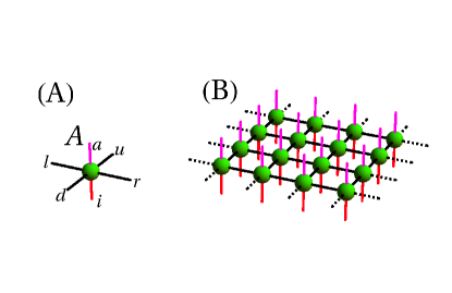
Figure 1: In A, graphic representation of the tensor $A^{ia}_{urdl}$. In B, the amplitude $\Psi_{A}[\{i,a\}]$ with all bond indices connecting nearest-neighbor tensors contracted. Here and in the following figures the index contraction is represented by a line connecting two tensors.

III Transverse field Quantum Ising model on a square lattice

We proceed with

$${\cal H}~{}=~{}-\sum_{\langle m,m^{\prime}\rangle}Z_{m}Z_{m^{\prime}}-h\sum_{m}X_{m}~{}\equiv~{}{\cal H}_{ZZ}+{\cal H}_{X}.$$ (6)

Here $Z,X$ are Pauli matrices. The model has a ferromagnetic phase with a non-zero spontaneous magnetization $\langle Z\rangle$ for small $h$ and large $\beta$. At $h=0$ the critical point is $\beta_{0}=-\ln(\sqrt{2}-1)/2=0.441$ and at zero temperature the quantum critical point is $h_{0}=3.044$, see Ref. hc .

IV Suzuki-Trotter decomposition

We define $U_{ZZ}(\Delta\beta)\equiv e^{-\frac{1}{2}{\cal H}_{ZZ}\Delta\beta}$ and $U_{X}(\Delta\beta)\equiv e^{-\frac{1}{2}{\cal H}_{X}\Delta\beta}$ for the interaction and the transverse field respectively. In the second-order Suzuki-Trotter decomposition a small time step is a product

$$U(d\beta)~{}=~{}U_{X}(d\beta/2)U_{ZZ}(d\beta)U_{X}(d\beta/2)~{}+~{}{\cal O}(d\beta^{3}).$$ (7)

The action of $U_{X}(d\beta/2)$ on PEPS replaces $A^{ia}_{urdl}$ with

$$\cosh\frac{hd\beta}{4}~{}A^{ia}_{urdl}~{}+~{}\sinh\frac{hd\beta}{4}~{}\sum_{j}X^{ij}A^{ja}_{urdl}$$ (8)

of the same bond dimension $D$.

The operator $U_{ZZ}(d\beta)$ is a product over nearest-neighbor bonds

$$U_{ZZ}(d\beta)=\prod_{\langle m,m^{\prime}\rangle}e^{\frac{d\beta}{2}Z_{m}Z_{m^{\prime}}}=$$

$$\prod_{\langle m,m^{\prime}\rangle}\cosh\frac{d\beta}{2}\sum_{s_{\langle m,m^{\prime}\rangle}=0,1}\Big{(}{\cal O}_{m}{\cal O}_{m^{\prime}}\Big{)}^{s_{\langle m,m^{\prime}\rangle}}$$ (9)

Here at each site $m$ we introduced ${\cal O}_{m}=Z_{m}\tanh^{1/2}\frac{d\beta}{2}$ and at each bond $\langle m,m^{\prime}\rangle$ a bond index $s_{\langle m,m^{\prime}\rangle}$. With the help of the bond indices, $U_{ZZ}(d\beta)$ can be rearranged as a tensor product operator, see Fig. 2, being a contraction of Trotter tensors,

$$T^{ij}_{s_{u},s_{r},s_{d},s_{l}}(d\beta)=\cosh^{2}\frac{d\beta}{2}~{}\left({\cal O}^{s}\right)^{ij},$$ (10)

through their bond indices $s_{u},s_{r},s_{d},s_{l}\in\left\{0,1\right\}$. Here $s=s_{u}+s_{r}+s_{d}+s_{l}$ is a sum of bond indices coming out from a given site. The action of the tensor product operator $U_{ZZ}(d\beta)$ maps $A$ to a new tensor

$$B^{ia}_{2u+s_{u},2r+s_{r},2d+s_{d},2l+s_{l}}=\sum_{j=0,1}T^{ij}_{s_{u},s_{r},s_{d},s_{l}}~{}A^{ja}_{urdl}$$ (11)

see Fig. 2B. This is an exact map, but $B$ has the bond dimension $2D$ instead of the original $D$.

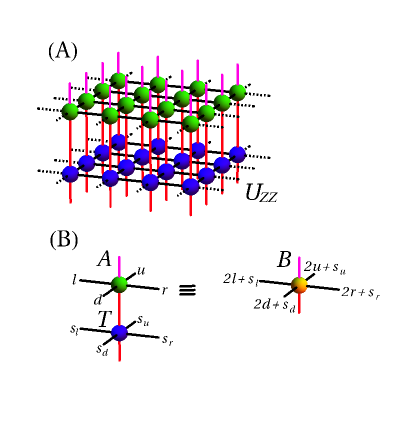
Figure 2: In A, the action of $U_{ZZ}(\beta)$ on the PEPS state in Fig. 1B. Here $U_{ZZ}$ is represented by a tensor product operator being a contraction of elementary Trotter tensors $T$. In B, each PEPS tensor $A$ can be fused with its Trotter tensor into a composite tensor $B$. Consequently, the application $U_{ZZ}$ to the original PEPS made of tensors $A$ results in a new PEPS made of tensors $B$ with a bond dimension $2D$. Its bond indices have to be renormalized back to the original dimension $D$.

V Tensor renormalization

The bond dimension has to be truncated back to $D$ in a way least distortive to the exact new PEPS $|\psi_{B}\rangle$. This renormalization can be done with an isometry $W$ that maps from $2D$ back to $D$ dimensions:

$$\sum_{u^{\prime},r^{\prime},d^{\prime},l^{\prime}=0}^{2D-1}W_{u}^{u^{\prime}}~{}W_{r}^{r^{\prime}}~{}W_{d}^{d^{\prime}}~{}W_{l}^{l^{\prime}}~{}B^{ia}_{u^{\prime}r^{\prime}d^{\prime}l^{\prime}}~{}=~{}A^{\prime ia}_{urdl}~{},$$ (12)

see Fig. 3. Here $A^{\prime}$ is a candidate for a new tensor after the infinitesimal time step with bond indices $u,r,d,l=0,...,D-1$. The isometry is a variational parameter and the renormalized new PEPS $|\psi_{A^{\prime}}\rangle$ is a function of this parameter. $W$ should maximize a fidelity

$$F=\langle\psi_{A^{\prime}}|\psi_{B}\rangle$$ (13)

between the exact $|\psi_{B}\rangle$ and the renormalized $|\psi_{A^{\prime}}\rangle$. From the point of view of numerical efficiency the fidelity has a disadvantage that it involves tensor $B$ with the doubled bond dimension. In the following, we optimize $A^{\prime}$ avoiding this overhead, but without compromising the accuracy of the second-order Suzuki-Trotter decomposition.

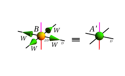
Figure 3: The action of the isometry $W$ on the exact new tensor $B$, compare Eq. (12). The isometry truncates the bond dimension from $2D$ back to the original $D$.

VI Self-consistent optimization

The maximization of the fidelity (13) with respect to $W$ can be done iteratively in a self-consistent way. We choose one bond in the bra $\langle\psi_{A^{\prime}}|$ and optimize the isometry on this bond keeping the isometries on all other bonds fixed. Once the chosen isometry is optimized, it is used to replace isometries on all other bonds as well. This optimization is repeated until convergence. Finally, the PEPS tensor $A^{\prime}$ in Eq. (12) with the converged $W$ is accepted as the new tensor after the infinitesimal time step.

In order to get rid of the numerical overhead introduced by tensor $B$, we note that when $W$ is already close enough to the optimal one, then $F$ will not be distorted much when we replace $|\psi_{B}\rangle$ with $|\psi_{A^{\prime}}\rangle$. In fact, when $D$ is large enough and $W$ is optimal, then it will not be distorted at all. After this replacement we arrive at a new figure of merit:

$$\langle\psi_{A^{\prime}}|\psi_{A^{\prime}}\rangle.$$ (14)

This is the norm of the PEPS with tensor $A^{\prime}$, but its maximization proceeds the same steps as the maximization of the fidelity (13). We choose one bond in the bra $\langle\psi_{A^{\prime}}|$ and optimize the isometry on this bond keeping isometries on all other bonds and the isometries in the ket $|\psi_{A^{\prime}}\rangle$ fixed. Once the chosen isometry is optimized, it is used to replace all other isometries as well, both in the bra and the ket. This optimization is repeated until convergence. Tensor $A^{\prime}$ with the converged $W$ is accepted as the new PEPS tensor after the infinitesimal time step.

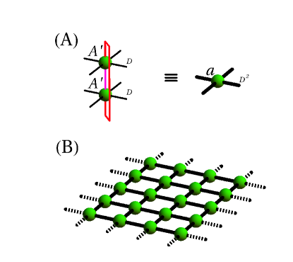
Figure 4: In A, tensor $A^{\prime}$ is contracted with its conjugate through their spin and ancilla indices. The contraction is a transfer tensor $a$. In B, a contraction of the transfer tensors is the norm $\langle\psi_{A^{\prime}}|\psi_{A^{\prime}}\rangle$ of the PEPS with tensor $A^{\prime}$. This infinite contraction can be done approximately with the help of the corner matrix renormalization CMR , see Appendix A.

Having outlined the algorithm, we still need to specify how to optimize the isometry on the chosen bond. To begin with, we note that a tensor network representing the norm (14) can be obtained as in Fig. 4. However, what we actually need is this norm, but with the chosen bond in the bra left uncontracted and its bond indices left unrenormalized by the isometry. This object can be obtained as in Fig. 5. We call it a “bond environment matrix” $E^{kl}$. Its indices are the unrenormalized and uncontracted bond indices along the chosen bond. From $E^{kl}$ we can obtain the norm by overlapping it with the projector $P^{kl}=\sum_{b=0}^{D-1}W^{k}_{b}W^{l}_{b}$ made of the isometry $W$:

$$\langle\psi_{A^{\prime}}|\psi_{A^{\prime}}\rangle=\sum_{k,l=0}^{2D-1}P^{kl}E^{kl}=\sum_{b=0}^{D-1}\sum_{k,l=0}^{2D-1}W^{k}_{b}W^{l}_{b}E^{kl}.$$ (15)

Here the isometries renormalize the uncontracted bond indices $k,l$ and then the sum over $b$ contracts the renormalized ones.

The norm (15) has to be maximized with respect to $W$ at fixed $E$. To this end, we diagonalize the symmetric $E$:

$$E^{kl}=\sum_{b=0}^{2D-1}V^{k}_{b}\lambda_{b}V^{l}_{b}$$ (16)

with eigenvalues $\lambda_{0}\geq...\geq\lambda_{2D-1}$. The optimal isometry is made of the leading eigenvectors:

$$W^{k}_{b}=V^{k}_{b}$$ (17)

for $b=0,...,D-1$. It maximizes the figure of merit (15) as $\langle\psi_{A^{\prime}}|\psi_{A^{\prime}}\rangle=\sum_{b=0}^{D-1}\lambda_{b}$.

Finally, we note that since the projector $P^{kl}$ is symmetric, in general only the symmetric part of $E^{kl}$ contributes to the norm (15) and, consequently, only the symmetric part has to be diagonalized in Eq. (16). This observation is used in Section VIII below.

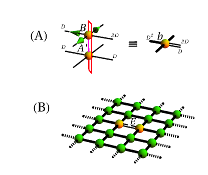
Figure 5: In A, a transfer tensor $b$ on a site at the chosen bond. In contrast to tensor $a$ in Fig. 4A, one of its bond indices along the chosen bond (the one within the bra) is left unrenormalized by the isometry. In B, the norm in Fig. 4B but with the chosen bond in the bra left uncontracted and its bond indices unrenormalized. This is a bond environment matrix $E$. This infinite tensor network is contracted by a method described in Appendix A.

VII Benchmark results

In order to evolve PEPS across the symmetry breaking phase transition we add to the Hamiltonian (6) a tiny longitudinal bias

$${\cal H}_{Z}=-\delta\sum_{s}Z_{s}$$ (18)

to smooth out the transition at a finite $\beta_{c}(h)$. We present results for the transverse field $h=\frac{2}{3}h_{c}$ that is large enough to introduce substantial quantum fluctuations and significantly increase $\beta_{c}$ above the Onsager’s $\beta_{0}$.

Figure 6 shows the order parameter $\langle Z\rangle$ as a function of $\beta$ for $\delta=10^{-6}$. The slope $d\langle Z\rangle/d\beta$ is the steepest at $\beta_{c}=0.589=1.33\beta_{0}$. This local observable requires $D\geq 6$ and a relatively small environmental bond dimension, $M\geq 12$, to converge.

Long range correlations are more demanding on $M$, as demonstrated by the ferromagnetic correlator in Fig. 7. For $\delta=10^{-6}$ we need $M\geq 20$ to converge a finite correlation length $\xi\approx 224$. It is finite thanks to the bias. As shown in Appendix C, $\delta=0$ would make both $\xi$ and necessary $M$ diverge at the critical point making accurate evolution across $\beta_{c}$ impossible.

Indeed, in Fig. 6 we also show $\langle Z\rangle$ obtained with $\delta=0$. Here the lack of convergence in $M$ manifests itself by a discontinuous jump in the spontaneous magnetization. Nevertheless, deeper in the ferromagnetic phase, where the influence of the bias becomes negligible, the magnetization overlaps with the smooth curve obtained with the tiny bias and converged in $M$.

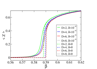
Figure 6: The ferromagnetic magnetization $\langle Z\rangle$ as a function of $\beta$ for the transverse field $h=\frac{2}{3}h_{0}$ and the longitudinal bias $\delta=10^{-6}$. This magnetization and other local observables are converged for $D\geq 6$ and $M\geq 12$. Here we show results for $M=16$. For comparison, we also show results without the bias field, $\delta=0$. Here the time step near $\beta_{c}$ is $d\beta=10^{-3}\beta_{0}=0.000441$.

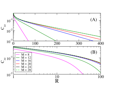
Figure 7: The ferromagnetic correlator, $C_{zz}(R)=\langle Z_{(x+R,y)}Z_{(x,y)}\rangle-\langle Z\rangle^{2}$, for the transverse field $h=\frac{2}{3}h_{c}$, the longitudinal bias $h_{Z}=10^{-6}$, at the critical $\beta_{c}=0.589$. The correlator is converged for $M\geq 24$ and $D\geq 6$. Here we show $D=6$. In A, a logarithmic plot emphasizing exponential tails for large $R$: $C_{zz}(R)\sim e^{-R/\xi}.$ The correlation length increases with $M$ until it converges at $\xi=224$ which is finite thanks to the finite bias. In B, a log-log plot emphasizing a power law decay for intermediate $R$, $C_{zz}(R)\sim R^{-\eta}.$ The best fit is $\eta=0.28$.

VIII Finite lattice

On a finite $N\times N$ lattice the self-consistent algorithm is basically the same as on the infinite one except that contraction of finite networks, like the one in Fig. 8, can be done with matrix product states OPS instead of the corner matrix renormalization in Appendix A. A finite lattice is also less symmetric than the infinite one, hence different bonds and their environments $E$ are not equivalent. One has to sweep across the lattice optimizing each bond separately - modulo residual symmetries - and repeat the sweeps until convergence of all bonds.

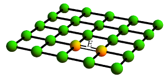
Figure 8: One of the bond environments on a $5\times 5$ lattice.

Figure 9 shows a ferromagnetic correlator along a diagonal of an $11\times 11$ lattice. The finite lattice size itself is enough to smooth the transition, hence there is no need for the longitudinal bias here and we set $\delta=0$.

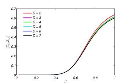
Figure 9: Ferromagnetic correlator $<Z_{3,3}Z_{9,9}>$ between sites $(3,3)$ and $(9,9)$ on a diagonal of an $11\times 11$ lattice as a function of $\beta$. Here the transverse field $g=\frac{2}{3}g_{c}$, the longitudinal bias $\delta=0$, and a bond dimension in the matrix product state is $M_{\rm MPS}=16$. The correlator is converged for bond dimension $D\geq 5$ and $M_{\rm MPS}\geq 16$.

IX Conclusion

We presented an iterative self-consistent renormalization of the PEPS bond dimension after a Suzuki-Trotter gate. The procedure takes into account full environment made of self-consistently renormalized tensors to preserve the accuracy of the Suzuki-Trotter decomposition. The algorithm is efficient: it takes one day in MATLAB on a laptop computer to obtain the data in this paper. Its formal cost - dominated by the corner matrix renormalization (CMR) - scales like $M^{3}D^{6}$, but in more efficient versions of CMR CMR it can be cut down to ${\cal O}(M^{3}D^{2})$. In conclusion, the protocol brings us closer to a numerically exact imaginary time evolution that can be used to obtain thermal states of strongly correlated systems.

Appendix A Corner matrix renormalization

An infinite tensor network, like the one on the left of Fig. 10, cannot be contracted exactly. Fortunately, what we need in general is not this number, but an environment for a few tensors of interest. For instance, in Fig. 10 we want an environment for the transfer tensor $a$ in the center. The environment is a tensor that remains after removing the central tensor from the infinite network. From the point of view of the central tensor, its environment can be substituted with an effective environment, made of finite corner matrices $C$ and top tensors $T$, that appears to the central tensor the same as the exact environment as much as possible. The environmental tensors are contracted with each other by indices of dimension $M$. Increasing $M$ makes the effective environment more accurate, and for a finite correlation length the environment is expected to converge at a finite $M$.

For the sake of simplicity, here in the Ising model, we assume that tensors $A,B,a$ are isotropic in their four bond indices. Consequently, $C$ is symmetric and top is symmetric in its environmental indices.

Finite tensors $C$ and $T$ represent infinite sectors of the network on the left of Fig. 10. The tensors are converged by iterating the corner matrix renormalization in Fig. 11. In every renormalization step, the corner matrix is enlarged with one tensor $a$ and two $T$’s. This operation represents the top-left corner sector in Fig. 10 absorbing one more layer of tensors $a$. Once the environment is converged, it can be used to calculate efficiently either observables or the bond environment $E$, see Fig. 12. Initialization of the iterative corner renormalization is discussed in Appendix B.

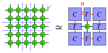
Figure 10: On the left, the norm $\langle\psi_{A}|\psi_{A}\rangle$ in Fig. 4B. This infinite contraction cannot be done exactly, hence it is approximated by the finite network on the right. Corner matrices $C$ and top tensors $T$ effectively represent corresponding infinite sectors of the network on the left separated by the dashed blue lines. Their (red) environmental bonds have dimension $M$. The environmental tensors $C$ and $T$ should be such that, to the transfer tensor $a$ in the center, its environment on the right appears the same as its exact environment on the left as much as possible. They are obtained by iterating the corner matrix renormalization in Fig. 11 until convergence.

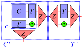
Figure 11: The corner $C$ and top $T$ are obtained by repeating a renormalization procedure until convergence. The procedure has four steps. In the first step, the tensors $C,T,a$ are contracted to an enlarged corner $C^{\prime\prime}$. In the second step, the symmetric $MD^{2}\times MD^{2}$ matrix $C^{\prime\prime}$ is diagonalized and its $M$ eigenvectors with the largest eigenvalues define an isometry $Z$. The diagonalization that scales like $M^{3}D^{6}$ is the leading cost of this variant of corner matrix renormalization. In the third step, $Z$ is used to renormalize/truncate the indices of $C^{\prime\prime}$ back to the original dimension $M$ giving a new (diagonal) corner $C^{\prime}$. In the fourth step, the same $Z$ renormalizes the contraction of $T$ with $a$ to a new $T^{\prime}$. The four-step procedure is repeated until convergence of the $M$ leading eigenvalues of $C^{\prime\prime}$.

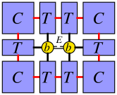
Figure 12: A finite network approximating the exact bond environment $E$ in Fig. 5C. For a finite correlation length, it is expected to become exact at a finite $M$.

Appendix B Gauge accelerator for corner matrix renormalization

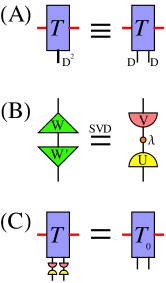
Figure 13: In A, the bottom index of tensor $T$ effectively comes out from tensor $a$, see Figs. 10 and 11. It is a fusion of two bond indices, each of dimension $D$, coming out from two tensors $A$, see Fig. 4A. Each bond index of tensor $A$ is actually a bond index of tensor $B$ renormalized by isometry $W$, see Fig. 3. In B, an overlap between old isometry $W$ and new $W^{\prime}$ is a $D\times D$ matrix. It can be subject to a singular value decomposition, $W^{\prime}W^{T}=U\lambda V^{T}$, with singular values $\lambda$. In C, an orthogonal matrix $UV^{T}$ is applied to each bottom index of the old tensor $T$. It is a gauge transformation that provides a better starting point $T_{0}$ for the iterative procedure in Fig. 11 converging the environmental tensors.

The iterative procedure in Fig. 11 converging the environmental tensors is the most time-consuming part of the algorithm. It is accelerated by using in the environment the renormalized tensor $A$ instead of the full tensor $B$, but at the price of repeating the self-consistent iterative update of $A$ (or equivalently $W$). Before every update of $A$, the environment has to be converged with current $A$. Once $A$ is updated, the environment has to be converged again with the updated $A$, and so forth until convergence of $A$. Fortunately, the convergence of the environment can be accelerated with a good choice of initial tensors $C_{0}$ and $T_{0}$. When $A$ is already close to convergence and it is changed little by its update, then the previous tensors $C$ and $T$, converged before the latest update of $A$, can be reused as the initial tensors. Moreover, they can be improved even further at negligible cost.

The update changes tensor $A$ by updating the isometry from an old $W$ to a new $W^{\prime}$. As explained in Fig. 13A, the bottom index of tensor $T$ is actually a fusion of two bond indices of two tensors $A$, and these bond indices are in fact bond indices of tensors $B$ renormalized by the old isometry $W$. We would like to replace this old $W$ with the new $W^{\prime}$ but, since $W$ is not invertible, this cannot be done exactly. However, as explained in Figs. 13B and C, we can apply an orthogonal (gauge) transformation to the bottom index of $T$ that is as close to the exact replacement $W\to W^{\prime}$ as possible. The transformed $T_{0}$ is a better starting point than the $T$ converged before the update of $W$.

Appendix C Onsager’s critical point at finite ${\bf M}$

In principle, a PEPS with a finite bond dimension $D$ can describe a finite-temperature critical point exactly. The best example is the Onsager’s phase transition at $\beta_{0}$ in the classical Ising model with $h=0=\delta$, where the exact PEPS tensor with $D=2$ is

$$A^{ia}_{s_{t},s_{r},s_{b},s_{l}}=T^{ia}_{s_{t},s_{r},s_{b},s_{l}}(\beta_{0}),$$ (19)

compare Eq. (10). Thus the problem at criticality is not a finite $D$ but a finite environmental bond dimension $M$, as demonstrated in Fig. 14, where we provide numerical evidence that the correlation length diverges with increasing $M$ roughly like $\xi\sim M^{2}$ and the spontaneous magnetization decays like $\xi^{-1/8}\sim M^{-1/4}$. Here $1/8$ is the scaling dimension. With increasing $M$ the effective environment does converge to the exact one but not at an exponential rate. Apparently, a finite $M$ cannot provide an accurate effective environment with an infinite correlation length.

For a nonzero transverse field $h$, the PEPS tensor at finite $\beta$ is obtained after a series of Suzuki-Trotter steps. An accurate step across the critical point requires an accurate effective environment that cannot be obtained with a finite $M$. We bypass this problem by adding a tiny longitudinal bias field that makes both the correlation length and the necessary $M$ finite.

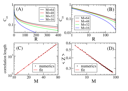
Figure 14: In A and B, the ferromagnetic correlator, $C_{zz}(R)=\langle Z_{(x+R,y)}Z_{(x,y)}\rangle-\langle Z\rangle^{2}$, at the critical $\beta_{c}=\beta_{0}$ in the classical Ising model with zero transverse field and longitudinal bias. The range of the correlator increases with the environmental bond dimension $M$. In A, a logarithmic plot emphasizing exponential tails for large $R$: $C_{zz}(R)\sim e^{-R/\xi}.$ The correlation length $\xi$ is shown in panel C. In B, a log-log plot emphasizing a power law decay for intermediate $1\ll R\ll\xi$, $C_{zz}(R)\sim R^{-\eta},$ converging to $\eta=1/4$ with increasing $M$. In C, the correlation length $\xi$ as a function of $M$. The best fit $\xi=1.05M^{1.93}$ suggests a power-law divergence with increasing $M$. In D, spontaneous magnetization $\langle Z\rangle$ as a function of $M$. The best fit $\langle Z\rangle=0.784M^{-0.246}$ suggests a power-law decay towards the exact $\langle Z\rangle=0$.