C-parameter Distribution at N3LL including Power Corrections

André H. Hoang University of Vienna, Faculty of Physics, Boltzmanngasse 5, A-1090 Wien, Austria Erwin Schrödinger International Institute for Mathematical Physics, University of Vienna, Boltzmanngasse 9, A-1090 Vienna, Austria    Daniel W. Kolodrubetz Center for Theoretical Physics, Massachusetts Institute of Technology, Cambridge, MA 02139, USA    Vicent Mateu University of Vienna, Faculty of Physics, Boltzmanngasse 5, A-1090 Wien, Austria    Iain W. Stewart Center for Theoretical Physics, Massachusetts Institute of Technology, Cambridge, MA 02139, USA
Abstract

We compute the e+esuperscript𝑒superscript𝑒e^{+}e^{-} C-parameter distribution using the Soft-Collinear Effective Theory with a resummation to N3LL accuracy of the most singular partonic terms. This includes the known fixed-order QCD results up to 𝒪(αs3)𝒪superscriptsubscript𝛼𝑠3\mathcal{O}(\alpha_{s}^{3}), a numerical determination of the two loop non-logarithmic term of the soft function, and all logarithmic terms in the jet and soft functions up to three loops. Our result holds for C𝐶C in the peak, tail, and far tail regions. Additionally, we treat hadronization effects using a field theoretic nonperturbative soft function, with moments ΩnsubscriptΩ𝑛\Omega_{n}. In order to eliminate an 𝒪(ΛQCD)𝒪subscriptΛQCD\mathcal{O}(\Lambda_{\rm QCD}) renormalon ambiguity in the soft function, we switch from the MS¯¯MS\overline{\rm MS} to a short distance “Rgap” scheme to define the leading power correction parameter Ω1subscriptΩ1\Omega_{1}. We show how to simultaneously account for running effects in Ω1subscriptΩ1\Omega_{1} due to renormalon subtractions and hadron-mass effects, enabling power correction universality between C-parameter and thrust to be tested in our setup. We discuss in detail the impact of resummation and renormalon subtractions on the convergence. In the relevant fit region for αs(mZ)subscript𝛼𝑠subscript𝑚𝑍\alpha_{s}(m_{Z}) and Ω1subscriptΩ1\Omega_{1}, the perturbative uncertainty in our cross section is 2.5%similar-to-or-equalsabsentpercent2.5\simeq 2.5\% at Q=mZ𝑄subscript𝑚𝑍Q=m_{Z}.

preprint: UWTHPH 2014-37 MIT–CTP 4596 LPN14-123

I Introduction

The study of event shape distributions in e+esuperscript𝑒superscript𝑒e^{+}\,e^{-} colliders has served as an excellent avenue to understand the structure of jets in QCD. Currently they also provide an important testing ground for new achievements in theoretical formalism, that can then also be extended to applications at hadron colliders. Moreover, event shapes provide accurate determinations of the strong coupling constant; see for example Refs. Bethke (2013) and Pich (2012). Experimentally they have been measured with high accuracy, and there exist perturbative computations at 𝒪(αs3)𝒪superscriptsubscript𝛼𝑠3\mathcal{O}(\alpha_{s}^{3}) Gehrmann-De Ridder et al. (2007a, b, 2009); Gehrmann-De Ridder et al. (2014); Weinzierl (2008, 2009). The use of the Soft-Collinear Effective Theory (SCET) Bauer et al. (2001a, b); Bauer and Stewart (2001); Bauer et al. (2002) has simplified the analysis of factorization theorems for event shapes Fleming et al. (2008a, b); Schwartz (2008); Bauer et al. (2008), enabling a resummation of large perturbative logs at next-to-next-to-next-to-leading log (N3LL) order and high-precision analyses for thrust and the heavy jet mass distributions Becher and Schwartz (2008); Chien and Schwartz (2010); Abbate et al. (2011, 2012). The corresponding factorization theorems have recently been extended to oriented event shapes in Mateu and Rodrigo (2013) and to account for the effects of virtual and real secondary massive quark radiation in Refs. Gritschacher et al. (2013); Pietrulewicz et al. (2014).

Our main motivations for studying the C-parameter distribution are to:

  • a)

    Extend the theoretical precision of the logarithmic resummation for C-parameter from next-to-leading log (NLL)+𝒪(αs3)𝒪superscriptsubscript𝛼𝑠3\,+\,{\cal O}(\alpha_{s}^{3}) to N3LL + 𝒪(αs3)𝒪superscriptsubscript𝛼𝑠3{\cal O}(\alpha_{s}^{3}).

  • b)

    Implement the leading power correction Ω1subscriptΩ1\Omega_{1} using only field theory and with sufficient theoretical precision to provide a serious test of universality between C-parameter and thrust.

  • c)

    Determine αs(mZ)subscript𝛼𝑠subscript𝑚𝑍\alpha_{s}(m_{Z}) using N3LL + 𝒪(αs3)+Ω1𝒪superscriptsubscript𝛼𝑠3subscriptΩ1{\cal O}(\alpha_{s}^{3})+\Omega_{1} theoretical precision for C𝐶C, to make this independent extraction competitive with the thrust analysis carried out at this level in Refs. Abbate et al. (2011, 2012).

In this article we present the theoretical calculation and analysis that yields a N3LL + 𝒪(αs3)+Ω1𝒪superscriptsubscript𝛼𝑠3subscriptΩ1{\cal O}(\alpha_{s}^{3})+\Omega_{1} cross section for C-parameter, and we analyze its convergence and perturbative uncertainties. A numerical analysis that obtains αs(mZ)subscript𝛼𝑠subscript𝑚𝑍\alpha_{s}(m_{Z}) from a fit to a global C-parameter dataset and investigates the power correction universality will be presented in a companion paper Hoang et al. (2015a). Preliminary versions of these results were presented in Refs. Dan (2013); Hoang et al. (2015b).

A nice property of C-parameter is that its definition does not involve any minimization procedure, unlike thrust. This makes its determination from data or Monte Carlo simulations computationally inexpensive. Unfortunately, this does not translate into a simplification of perturbative theoretical computations, which are similar to those for thrust.

The resummation of singular logarithms in C-parameter was first studied by Catani and Webber in Ref. Catani and Webber (1998) using the coherent branching formalism Catani et al. (1993), where NLL accuracy was achieved. Making use of SCET in this article, we achieve a resummation at N3LL order. The relation between thrust and C-parameter in SCET discussed here has been used in the Monte Carlo event generator GENEVA Alioli et al. (2013), where a next-to-next-to-leading log primed (N2LL) C-parameter result was presented. Nonperturbative effects for the C-parameter distribution have been studied by a number of authors: Gardi and Magnea Gardi and Magnea (2003), in the context of the dressed gluon approximation; Korchemsky and Tafat Korchemsky and Tafat (2000), in the context of a shape function; and Dokshitzer and Webber Dokshitzer and Webber (1995), in the context of the dispersive model.

Catani and WebberCatani and Webber (1998) showed that up to NLL the cross sections for thrust and the reduced C-parameter

C~=C6,~𝐶𝐶6\displaystyle\widetilde{C}=\frac{C}{6}\,, (1)

are identical. Gardi and Magnea Gardi and Magnea (2003) showed that this relation breaks down beyond NLL due to soft radiation at large angles. Using SCET we confirm and extend these observations by demonstrating that the hard and jet functions, along with all anomalous dimensions, are identical for thrust and C~~𝐶\widetilde{C} to all orders in perturbation theory. At any order in perturbation theory, the perturbative non-universality of the singular terms appears only through fixed-order terms in the soft function, which differ starting at 𝒪(αs)𝒪subscript𝛼𝑠\mathcal{O}(\alpha_{s}).

There is also a universality between the leading power corrections for thrust and C-parameter which has been widely discussed Dokshitzer and Webber (1995); Akhoury and Zakharov (1995); Korchemsky and Sterman (1995); Lee and Sterman (2007). This universality has been proven nonperturbatively in Ref. Lee and Sterman (2007) using the field theory definition of the leading power correction with massless particle kinematics. In our notation this relation is

Ω1C=3π2Ω1τ.superscriptsubscriptΩ1𝐶3𝜋2superscriptsubscriptΩ1𝜏\displaystyle\Omega_{1}^{C}=\frac{3\pi}{2}\,\Omega_{1}^{\tau}\,. (2)

Here Ω1esuperscriptsubscriptΩ1𝑒\Omega_{1}^{e} is the first moment of the nonperturbative soft functions for the event shape e𝑒e and, in the tail of the distribution acts to shift the event shape variable

σ^(e)σ^(eΩ1e/Q),^𝜎𝑒^𝜎𝑒superscriptsubscriptΩ1𝑒𝑄\displaystyle\hat{\sigma}(e)\to\hat{\sigma}(e-\Omega_{1}^{e}/Q)\,, (3)

at leading power. The exact equality in Eq. (2) can be spoiled by hadron-mass effects Salam and Wicke (2001), which have been formulated using a field theoretic definition of the Ω1esuperscriptsubscriptΩ1𝑒\Omega_{1}^{e} parameters in Ref. Mateu et al. (2013). Even though nonzero hadron masses can yield quite large effects for some event shapes, the universality breaking corrections between thrust and C-parameter are at the 2.5%percent2.52.5\% level and hence for our purposes are small relative to other uncertainties related to determining Ω1subscriptΩ1\Omega_{1}. Since relations like Eq. (2) do not hold for higher moments Ωn>1esuperscriptsubscriptΩ𝑛1𝑒\Omega_{n>1}^{e} of the nonperturative soft functions, these are generically different for thrust and C-parameter.

Following Ref. Abbate et al. (2011), a rough estimate of the impact of power corrections can be obtained from the experimental data with very little theoretical input. We write (1/σ)dσ/dCh(CΩ1C/Q)=h(C)h(C)Ω1C/Q+similar-to-or-equals1𝜎d𝜎d𝐶𝐶superscriptsubscriptΩ1𝐶𝑄𝐶superscript𝐶superscriptsubscriptΩ1𝐶𝑄(1/\sigma)\,\mathrm{d}\sigma/\mathrm{d}C\simeq h(C-\Omega_{1}^{C}/Q)=h(C)-h^{\prime}(C)\,\Omega_{1}^{C}/Q+\ldots for the tail region, and assume the perturbative function h(C)𝐶h(C) is proportional to αssubscript𝛼𝑠\alpha_{s}. Then one can easily derive that if a value αssubscript𝛼𝑠\alpha_{s} is extracted from data by setting Ω1C=0superscriptsubscriptΩ1𝐶0\Omega_{1}^{C}=0 then the change in the extracted value δαs𝛿subscript𝛼𝑠\delta\alpha_{s} when Ω1CsuperscriptsubscriptΩ1𝐶\Omega_{1}^{C} is present will be

δαsαsΩ1CQh(C)h(C),similar-to-or-equals𝛿subscript𝛼𝑠subscript𝛼𝑠superscriptsubscriptΩ1𝐶𝑄superscript𝐶𝐶\displaystyle\frac{\delta\alpha_{s}}{\alpha_{s}}\simeq\frac{\Omega_{1}^{C}}{Q}\>\frac{h^{\prime}(C)}{h(C)}\,, (4)

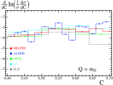
where the slope factor h(C)/h(C)superscript𝐶𝐶h^{\prime}(C)/h(C) should be constant at the level of these approximations. By looking at the experimental results at the Z-pole shown in Fig. 1, we see that this is true at the level expected from these approximations, finding h(C)/h(C) 3.3±0.8similar-to-or-equalssuperscript𝐶𝐶plus-or-minus3.30.8h^{\prime}(C)/h(C)\simeq-\,3.3\pm 0.8. This same analysis for thrust T=1τ𝑇1𝜏T=1-\tau involves a different function hh and yields [h(τ)/h(τ)]τ 14±4similar-to-or-equalssubscriptdelimited-[]superscript𝜏𝜏𝜏plus-or-minus144[h^{\prime}(\tau)/h(\tau)]_{\tau}\simeq-\,14\pm 4 Abbate et al. (2011). It is interesting to note that even this very simple analysis gives a value [h(τ)/h(τ)]τ/[h(C)/h(C)]C4.2similar-to-or-equalssubscriptdelimited-[]superscript𝜏𝜏𝜏subscriptdelimited-[]superscript𝐶𝐶𝐶4.2[\,h^{\prime}(\tau)/h(\tau)\,]_{\tau}/[\,h^{\prime}(C)/h(C)\,]_{C}\simeq 4.2 that is very close to the universality prediction of 3π/2=4.73𝜋24.73\pi/2=4.7. In the context of Eq. (2), this already implies that in a C-parameter analysis we can anticipate the impact of the power correction in the extraction of the strong coupling to be quite similar to that in the thrust analysis Abbate et al. (2011), where δαs/αs 9%similar-to-or-equals𝛿subscript𝛼𝑠subscript𝛼𝑠percent9\delta\alpha_{s}/\alpha_{s}\simeq-\,9\%.

Refer to caption
Figure 1: Plot of d/dCln[(1/σ)dσ/dC]h(C)/h(C)similar-to-or-equalsdd𝐶1𝜎d𝜎d𝐶superscript𝐶𝐶\mathrm{d}/\mathrm{d}C\,\ln[(1/\sigma)\mathrm{d}\sigma/\mathrm{d}C]\simeq h^{\prime}(C)/h(C), computed from experimental data at Q=mZ𝑄subscript𝑚𝑍Q=m_{Z}. The derivative is calculated using the central difference with neighboring points.

In Ref. Catani and Webber (1997) it was shown that within perturbation theory the C-parameter distribution reaches an infinite value at a point in the physical spectrum 0<C<10𝐶10<C<1, despite being an infrared and collinear safe observable. This happens for the configuration that distinguishes planar and non-planar partonic events and first occurs at 𝒪(αs2)𝒪superscriptsubscript𝛼𝑠2\mathcal{O}(\alpha_{s}^{2}) where one has enough partons to create a non-planar event at the value Cshoulder=3/4subscript𝐶shoulder34C_{\rm shoulder}=3/4. However, this singularity is integrable and related to the fact that at 𝒪(αs)𝒪subscript𝛼𝑠\mathcal{O}(\alpha_{s}) the cross section does not vanish at the three-parton endpoint Cshouldersubscript𝐶shoulderC_{\rm shoulder}. In Ref. Catani and Webber (1997) this deficiency was cured by performing soft gluon resummation at Cshouldersubscript𝐶shoulderC_{\rm shoulder} to achieve a smooth distribution at leading-log (LL) order. Since Cshouldersubscript𝐶shoulderC_{\rm shoulder} is far away from the dijet limit (in fact, it is a pure three-jet configuration), we will not include this resummation. In our analysis the shoulder effect is included in the non-singular contributions in fixed-order, and when the partonic distribution is convoluted with a nonperturbative shape function, the shoulder effect is smoothed out, providing a continuous cross section across the entire C𝐶C range.

This paper is organized as follows: In Sec. II we review the definition of C-parameter and highlight some of its properties and relations to other event shapes, and in Sec. III we study simplifications that occur for the calculation of C-parameter when we consider soft and collinear radiation in the dijet limit. These simplifications are necessary to derive the C-parameter factorization theorem and to address the question of which perturbative objects are common with thrust. In Sec. IV we establish the factorization theorem for C𝐶C and show how to perform large log resummation using the renormalization group evolution (RGE). Some details on the form of the kinematically power suppressed terms known as nonsingular contributions to the C-parameter distribution are discussed in Sec. V, and in Sec. VI we show results for our numerical determination of the non-logarithmic coefficients of the two-loop soft function. Section VII contains a presentation of the form of the nonperturbative power corrections and their definition in a renormalon-free scheme. Our method to implement scale variation using profile functions is discussed in Sec. VIII. In Sec. IX we present our main results for the C-parameter cross section, including the impact of the resummation slope parameter, the convergence of the resummed perturbation theory, and the perturbative theoretical uncertainties. In Sec. X we give the conclusions and an outlook.

The work contains seven appendices: Appendix A provides all needed formulae for the singular cross section beyond those in the main body of the paper. In App. B we present a comparison of our SCET prediction, expanded at fixed order, with the numerical results in full QCD at 𝒪(αs2)𝒪superscriptsubscript𝛼𝑠2\mathcal{O}(\alpha_{s}^{2}) and 𝒪(αs3)𝒪superscriptsubscript𝛼𝑠3\mathcal{O}(\alpha_{s}^{3}) from EVENT2 and EERAD3, respectively. In App. C we give a general formula for the one-loop soft function, valid for any event shape which is not recoil sensitive. In App. D we give analytic expressions for the Bisubscript𝐵𝑖B_{i} and Gijsubscript𝐺𝑖𝑗G_{ij} coefficients of the fixed-order singular logs up to 𝒪(αs3)𝒪superscriptsubscript𝛼𝑠3\mathcal{O}(\alpha_{s}^{3}) according to the exponential formula of Sec. IX.1. The R-evolution of the renormalon-free gap parameter is described in App. E. Appendix F is devoted to a discussion of how the Rgap scheme is handled in the shoulder region above Cshoulder=3/4subscript𝐶shoulder34C_{\rm shoulder}=3/4. Finally, in App. G we show results for the perturbative gap subtraction series based on the C-parameter soft function.

II Definition and properties of C-parameter

C-parameter is defined in terms of the linearized momentum tensor Parisi (1978); Donoghue et al. (1979),

Θαβ=1i|pi|ipiαpiβ|pi|,superscriptΘ𝛼𝛽1subscript𝑖subscript𝑝𝑖subscript𝑖superscriptsubscript𝑝𝑖𝛼superscriptsubscript𝑝𝑖𝛽subscript𝑝𝑖\displaystyle\Theta^{\alpha\beta}\,=\,\frac{1}{\sum_{i}|{\vec{p}}_{i}|}\sum_{i}\frac{p_{i}^{\alpha}p_{i}^{\beta}}{|{\vec{p}}_{i}|}\,, (5)

where α=1,2,3𝛼123\alpha=1,2,3 are spacial indices and i𝑖i sums over all final state particles. Since ΘΘ\Theta is a symmetric positive semi-definite matrix 111This property follows trivially from Eq. (5), since for any three-vector q𝑞\vec{q} one has that qαqβΘαβi(qpi)2/|pi|0proportional-tosubscript𝑞𝛼subscript𝑞𝛽superscriptΘ𝛼𝛽subscript𝑖superscript𝑞subscript𝑝𝑖2subscript𝑝𝑖0q_{\alpha}q_{\beta}\Theta^{\alpha\beta}\propto\sum_{i}({\vec{q}}\cdot{\vec{p}}_{i})^{2}/|{\vec{p}}_{i}|\geq 0., its eigenvalues are real and non-negative. Let us denote them by λisubscript𝜆𝑖\lambda_{i}, i=1,2,3𝑖123i=1,2,3. As ΘΘ\Theta has unit trace, iλi=1subscript𝑖subscript𝜆𝑖1\sum_{i}\lambda_{i}=1, which implies that the eigenvalues are bounded 0λi10subscript𝜆𝑖10\leq\lambda_{i}\leq 1. Without loss of generality we can assume 1λ1λ2λ301subscript𝜆1subscript𝜆2subscript𝜆301\geq\lambda_{1}\geq\lambda_{2}\geq\lambda_{3}\geq 0. The characteristic polynomial for the eigenvalues of ΘΘ\Theta is:

x3x2+(λ1λ2+λ1λ3+λ2λ3)xλ1λ2λ3=0.superscript𝑥3superscript𝑥2subscript𝜆1subscript𝜆2subscript𝜆1subscript𝜆3subscript𝜆2subscript𝜆3𝑥subscript𝜆1subscript𝜆2subscript𝜆30\displaystyle x^{3}-x^{2}+(\lambda_{1}\lambda_{2}+\lambda_{1}\lambda_{3}+\lambda_{2}\lambda_{3})\,x-\lambda_{1}\lambda_{2}\lambda_{3}=0\,. (6)

C-parameter is defined to be proportional to the coefficient of the term linear in x𝑥x:

C𝐶\displaystyle C =3(λ1λ2+λ1λ3+λ2λ3)absent3subscript𝜆1subscript𝜆2subscript𝜆1subscript𝜆3subscript𝜆2subscript𝜆3\displaystyle=3\,(\lambda_{1}\lambda_{2}+\lambda_{1}\lambda_{3}+\lambda_{2}\lambda_{3}) (7)
=3[(λ1+λ2)(1λ1)λ22],absent3delimited-[]subscript𝜆1subscript𝜆21subscript𝜆1superscriptsubscript𝜆22\displaystyle=3\,[\,(\lambda_{1}+\lambda_{2})(1-\lambda_{1})-\lambda_{2}^{2}\,]\,,

where we have used the unit trace property to write λ3subscript𝜆3\lambda_{3} in terms of λ1subscript𝜆1\lambda_{1} and λ2subscript𝜆2\lambda_{2} in order to get the second line. Similarly one defines D-parameter as D=27λ1λ2λ3𝐷27subscript𝜆1subscript𝜆2subscript𝜆3D=27\,\lambda_{1}\lambda_{2}\lambda_{3}, proportional to the x𝑥x-independent term in the characteristic equation. Trivially one also finds that

Tr[Θ2]=iλi2=123C,Trdelimited-[]superscriptΘ2subscript𝑖superscriptsubscript𝜆𝑖2123𝐶\displaystyle{\rm Tr}\,[\,\Theta^{2}\,]=\sum_{i}\lambda_{i}^{2}=1\,-\,\frac{2}{3}\,C\,, (8)

where again we have used λ3=1λ1λ2subscript𝜆31subscript𝜆1subscript𝜆2\lambda_{3}=1\,-\,\lambda_{1}\,-\,\lambda_{2}. We can easily compute Tr[Θ2]Trdelimited-[]superscriptΘ2{\rm Tr}\,[\,\Theta^{2}\,] using Eq. (5)

Tr[Θ2]Trdelimited-[]superscriptΘ2\displaystyle{\rm Tr}\,[\,\Theta^{2}\,] =1(i|pi|)2ij(pipj)2|pi||pj|absent1superscriptsubscript𝑖subscript𝑝𝑖2subscript𝑖𝑗superscriptsubscript𝑝𝑖subscript𝑝𝑗2subscript𝑝𝑖subscript𝑝𝑗\displaystyle=\frac{1}{(\sum_{i}|{\vec{p}}_{i}|)^{2}}\sum_{ij}\frac{({\vec{p}}_{i}\cdot{\vec{p}}_{j})^{2}}{|{\vec{p}}_{i}||{\vec{p}}_{j}|} (9)
=1(i|pi|)2ij|pi||pj|cos2θijabsent1superscriptsubscript𝑖subscript𝑝𝑖2subscript𝑖𝑗subscript𝑝𝑖subscript𝑝𝑗superscript2subscript𝜃𝑖𝑗\displaystyle=\frac{1}{(\sum_{i}|{\vec{p}}_{i}|)^{2}}\sum_{ij}|{\vec{p}}_{i}||{\vec{p}}_{j}|\cos^{2}\theta_{ij}
=11(i|pi|)2ij|pi||pj|sin2θij.absent11superscriptsubscript𝑖subscript𝑝𝑖2subscript𝑖𝑗subscript𝑝𝑖subscript𝑝𝑗superscript2subscript𝜃𝑖𝑗\displaystyle=1\,-\,\frac{1}{(\sum_{i}|{\vec{p}}_{i}|)^{2}}\sum_{ij}|{\vec{p}}_{i}||{\vec{p}}_{j}|\sin^{2}\theta_{ij}\,.

From the last relation one gets the familiar expression:

C=32i,j|pi||pj|sin2θij(i|pi|)2.𝐶32subscript𝑖𝑗subscript𝑝𝑖subscript𝑝𝑗superscript2subscript𝜃𝑖𝑗superscriptsubscript𝑖subscript𝑝𝑖2C=\frac{3}{2}\,\frac{\sum_{i,j}|\vec{p}_{i}||\vec{p}_{j}|\sin^{2}\theta_{ij}}{\left(\sum_{i}|\vec{p}_{i}|\right)^{2}}\,. (10)

From Eq. (10) and the properties of λisubscript𝜆𝑖\lambda_{i}, it follows that C0𝐶0C\geq 0, and from the second line of Eq. (7), one finds that C1𝐶1C\leq 1, and the maximum value is achieved for the symmetric configuration λ1=λ2=λ3=1/3subscript𝜆1subscript𝜆2subscript𝜆313\lambda_{1}=\lambda_{2}=\lambda_{3}=1/3. Hence, 0C10𝐶10\leq C\leq 1. Planar events have λ3=0subscript𝜆30\lambda_{3}=0. To see this simply consider that the planar event defines the xy𝑥𝑦x-y plane, and then any vector in the z𝑧z direction is an eigenstate of ΘΘ\Theta with zero eigenvalue. Hence, planar events have D=0𝐷0D=0 and C=3λ1(1λ1)𝐶3subscript𝜆11subscript𝜆1C=3\,\lambda_{1}\,(1-\lambda_{1}), which gives a maximum value for λ1=λ2=1/2subscript𝜆1subscript𝜆212\lambda_{1}=\lambda_{2}=1/2, and one has 0Cplanar3/40subscript𝐶planar340\leq C_{\rm planar}\leq 3/4. Thus C>3/4𝐶34C>3/4 needs at least four particles in the final state. C-parameter is related to the first non-trivial Fox–Wolfram parameter Fox and Wolfram (1978). The Fox–Wolfram event shapes are defined as follows:

H=ij|pi||pj|Q2P(cosθij).subscript𝐻subscript𝑖𝑗subscript𝑝𝑖subscript𝑝𝑗superscript𝑄2subscript𝑃subscript𝜃𝑖𝑗\displaystyle H_{\ell}=\sum_{ij}\frac{|\vec{p}_{i}||\vec{p}_{j}|}{Q^{2}}\,P_{\ell}(\cos\theta_{ij})\,. (11)

One has H0=1subscript𝐻01H_{0}=1, H1=0subscript𝐻10H_{1}=0, and

H2=1321Q2ij|pi||pj|sin2θij,subscript𝐻21321superscript𝑄2subscript𝑖𝑗subscript𝑝𝑖subscript𝑝𝑗superscript2subscript𝜃𝑖𝑗\displaystyle H_{2}=1-\frac{3}{2}\,\frac{1}{Q^{2}}\sum_{ij}|\vec{p}_{i}||\vec{p}_{j}|\sin^{2}\theta_{ij}\,, (12)

which is similar to Eq. (10). It turns out that for massless partonic particles they are related in a simple way: H2= 1Cpartsubscript𝐻21subscript𝐶partH_{2}\,=\,1\,-\,C_{\rm part}. As a closing remark, we note that for massless particles C-parameter can be easily expressed in terms of scalar products with four vectors:

Cpart=3321Q2ij(pipj)2EiEj.subscript𝐶part3321superscript𝑄2subscript𝑖𝑗superscriptsubscript𝑝𝑖subscript𝑝𝑗2subscript𝐸𝑖subscript𝐸𝑗\displaystyle C_{\rm part}=3-\frac{3}{2}\,\frac{1}{Q^{2}}\sum_{ij}\frac{(p_{i}\cdot p_{j})^{2}}{E_{i}E_{j}}\,. (13)

III C-Parameter Kinematics in the Dijet Limit

We now show that in a dijet configuration with only soft 222In this paper, for simplicity we denote as soft particles what are sometimes called ultrasoft particles in SCETI., n𝑛n-collinear, and n¯¯𝑛\bar{n}-collinear particles, the value of C-parameter can, up to corrections of higher power in the SCET counting parameter λ𝜆\lambda, be written as the sum of contributions from these three kinds of particles:

Cdijet=Cn+Cn¯+Cs+𝒪(λ4).subscript𝐶dijetsubscript𝐶𝑛subscript𝐶¯𝑛subscript𝐶s𝒪superscript𝜆4\displaystyle C_{\rm dijet}=C_{n}+C_{\bar{n}}+C_{\rm s}+\mathcal{O}(\lambda^{4})\,. (14)

To that end we define

Cdijetsubscript𝐶dijet\displaystyle C_{\rm dijet} =Cn,n+Cn¯,n¯+2Cn,n¯+2Cn,s+2Cn¯,s+Cs,s,absentsubscript𝐶𝑛𝑛subscript𝐶¯𝑛¯𝑛2subscript𝐶𝑛¯𝑛2subscript𝐶𝑛s2subscript𝐶¯𝑛ssubscript𝐶ss\displaystyle=C_{n,n}+C_{\bar{n},\bar{n}}+2\,C_{n,\bar{n}}+2\,C_{n,\rm s}+2\,C_{\bar{n},\rm s}+C_{\rm s,s}\,,
Ca,bsubscript𝐶𝑎𝑏\displaystyle C_{a,b} 321(i|pi|)2ia,jb|pi||pj|sin2θij.absent321superscriptsubscript𝑖subscript𝑝𝑖2subscriptformulae-sequence𝑖𝑎𝑗𝑏subscript𝑝𝑖subscript𝑝𝑗superscript2subscript𝜃𝑖𝑗\displaystyle\equiv\frac{3}{2}\,\frac{1}{\left(\sum_{i}|\vec{p}_{i}|\right)^{2}}\!\!\sum_{i\in a,j\in b}\!|\vec{p}_{i}||\vec{p}_{j}|\sin^{2}\theta_{ij}\,. (15)

The various factors of 222 take into account that for ab𝑎𝑏a\neq b one has to add the symmetric term ab𝑎𝑏a\leftrightarrow b.

The SCETIsubscriptSCETI\rm SCET_{I} power counting rules imply the following scaling for momenta: psμQλ2similar-tosuperscriptsubscript𝑝s𝜇𝑄superscript𝜆2p_{\rm s}^{\mu}\sim Q\,\lambda^{2}, pnQ(λ2,1,λ)similar-tosubscript𝑝𝑛𝑄superscript𝜆21𝜆p_{n}\sim Q\,(\lambda^{2},1,\lambda), pn¯Q(1,λ2,λ)similar-tosubscript𝑝¯𝑛𝑄1superscript𝜆2𝜆p_{\bar{n}}\sim Q\,(1,\lambda^{2},\lambda), where we use the light-cone components pμ=(p+,p,p)superscript𝑝𝜇superscript𝑝superscript𝑝subscript𝑝perpendicular-top^{\mu}=(p^{+},p^{-},p_{\perp}). Each one of the terms in Eq. (III), as well as Cdijetsubscript𝐶dijetC_{\rm dijet} itself, can be expanded in powers of λ𝜆\lambda:

Ca,b=i=0Ca,b(i),Ca,b(i)𝒪(λi+2).formulae-sequencesubscript𝐶𝑎𝑏subscript𝑖0superscriptsubscript𝐶𝑎𝑏𝑖similar-tosuperscriptsubscript𝐶𝑎𝑏𝑖𝒪superscript𝜆𝑖2\displaystyle C_{a,b}=\sum_{i=0}C_{a,b}^{(i)}\,,\quad C_{a,b}^{(i)}\sim\mathcal{O}(\lambda^{i+2})\,. (16)

The power counting implies that Cdijetsubscript𝐶dijetC_{\rm dijet} starts at 𝒪(λ2)𝒪superscript𝜆2\mathcal{O}(\lambda^{2}) and Cs,ssubscript𝐶ssC_{\rm s,\rm s} is a power correction since Cs,s(0)=0superscriptsubscript𝐶𝑠𝑠00C_{s,s}^{(0)}=0, while Cs,s(2)0superscriptsubscript𝐶𝑠𝑠20C_{s,s}^{(2)}\neq 0. All nlimit-from𝑛n- and n¯¯𝑛{\bar{n}}-collinear particles together will be denoted as the collinear particles with c=nn¯𝑐𝑛¯𝑛c=n\cup\bar{n}. The collinear particles have masses much smaller than Qλ𝑄𝜆Q\,\lambda and can be taken as massless at leading power. For soft particles we have perturbative components that can be treated as massless when Qλ2ΛQCDmuch-greater-than𝑄superscript𝜆2subscriptΛQCDQ\lambda^{2}\gg\Lambda_{\rm QCD}, and nonperturbative components that always should be treated as massive. Also at leading order one can use i|pi|=ic|pi|+𝒪(λ2)=Q+𝒪(λ2)subscript𝑖subscript𝑝𝑖subscript𝑖csubscript𝑝𝑖𝒪superscript𝜆2𝑄𝒪superscript𝜆2\sum_{i}|\vec{p}_{i}|=\sum_{i\in\rm c}|\vec{p}_{i}|+\mathcal{O}(\lambda^{2})=Q+\mathcal{O}(\lambda^{2}) and |pic|=Eic+𝒪(λ2)subscript𝑝𝑖csubscript𝐸𝑖c𝒪superscript𝜆2|\vec{p}_{i\in\rm c}|=E_{i\in\rm c}+\mathcal{O}(\lambda^{2}).

Defining Cs2Cn,s+2Cn¯,ssubscript𝐶𝑠2subscript𝐶𝑛s2subscript𝐶¯𝑛sC_{s}\equiv 2\,C_{n,\rm s}+2\,C_{\bar{n},\rm s} we find,

Cssubscript𝐶𝑠\displaystyle C_{s} =3Q2ic,js|pi||pj|sin2θijabsent3superscript𝑄2subscriptformulae-sequence𝑖c𝑗ssubscript𝑝𝑖subscript𝑝𝑗superscript2subscript𝜃𝑖𝑗\displaystyle\,=\,\frac{3}{Q^{2}}\!\!\!\sum_{i\in{\rm c},j\in{\rm s}}\!\!\!|\vec{p}_{i}||\vec{p}_{j}|\sin^{2}\theta_{ij} (17)
=3Q2ic|pi|js|pj|[sin2θj+O(λ2)]absent3superscript𝑄2subscript𝑖csubscript𝑝𝑖subscript𝑗ssubscript𝑝𝑗delimited-[]superscript2subscript𝜃𝑗𝑂superscript𝜆2\displaystyle=\frac{3}{Q^{2}}\!\sum_{i\in\rm c}|\vec{p}_{i}|\sum_{j\in\rm s}|\vec{p}_{j}|\big{[}\sin^{2}\theta_{j}+O(\lambda^{2})\,\big{]}
=3Qjs(pj)2|pj|+O(λ4)=3Qjspjcoshηj+O(λ4),absent3𝑄subscript𝑗ssuperscriptsuperscriptsubscript𝑝𝑗perpendicular-to2subscript𝑝𝑗𝑂superscript𝜆43𝑄subscript𝑗ssuperscriptsubscript𝑝𝑗perpendicular-tosubscript𝜂𝑗𝑂superscript𝜆4\displaystyle=\frac{3}{Q}\!\sum_{j\in\rm s}\frac{(p_{j}^{\perp})^{2}}{|\vec{p}_{j}|}+O(\lambda^{4})=\frac{3}{Q}\sum_{j\in\rm s}\frac{p_{j}^{\perp}}{\cosh\eta_{j}}+O(\lambda^{4})\,,

where the last displayed term will be denoted as Cs(0)superscriptsubscript𝐶𝑠0C_{s}^{(0)}. Here θjsubscript𝜃𝑗\theta_{j} is the angle between the three-momenta of a particle and the thrust axis and hence is directly related to the pseudorapidity ηjsubscript𝜂𝑗\eta_{j}. Also pj|pj|superscriptsubscript𝑝𝑗perpendicular-tosubscriptsuperscript𝑝perpendicular-to𝑗p_{j}^{\perp}\equiv|\vec{p}^{\,\perp}_{j}| is the magnitude of the three-momentum projection normal to the thrust axis. To get to the second line, we have used that sinθij=sinθj+O(λ2)subscript𝜃𝑖𝑗subscript𝜃𝑗𝑂superscript𝜆2\sin\theta_{ij}=\sin\theta_{j}\,+\,O(\lambda^{2}), and to get the last line, we have used sinθj=pj/|pj|=1/coshηjsubscript𝜃𝑗subscriptsuperscript𝑝perpendicular-to𝑗subscript𝑝𝑗1subscript𝜂𝑗\sin\theta_{j}=p^{\perp}_{j}/|\vec{p}_{j}\,|=1/\cosh\eta_{j}. In order to compute the partonic soft function, it is useful to consider Cs(0)superscriptsubscript𝐶𝑠0C_{s}^{(0)} for the case of massless particles:

Cs(0)|m=0=6Qjspj+pjpj++pj.evaluated-atsuperscriptsubscript𝐶𝑠0m06𝑄subscript𝑗ssuperscriptsubscript𝑝𝑗superscriptsubscript𝑝𝑗superscriptsubscript𝑝𝑗superscriptsubscript𝑝𝑗\displaystyle C_{s}^{(0)}\Big{|}_{\rm m=0}=\frac{6}{Q}\sum_{j\in\rm s}\frac{p_{j}^{+}p_{j}^{-}}{p_{j}^{+}+p_{j}^{-}}\,. (18)

Let us next consider Cn,nsubscript𝐶𝑛𝑛C_{n,n} and Cn¯,n¯subscript𝐶¯𝑛¯𝑛C_{\bar{n},\bar{n}}. Using energy conservation and momentum conservation in the thrust direction one can show that, up to 𝒪(λ2)𝒪superscript𝜆2\mathcal{O}(\lambda^{2}), En=En¯=Q/2subscript𝐸𝑛subscript𝐸¯𝑛𝑄2E_{n}=E_{\bar{n}}=Q/2. All n𝑛n-collinear particles are in the plus-hemisphere, and all the n¯¯𝑛\bar{n}-collinear particles are in the minus-hemisphere. Here the plus- and minus-hemispheres are defined by the thrust axis. For later convenience we define aμ=iapiμsuperscriptsubscript𝑎𝜇subscript𝑖𝑎superscriptsubscript𝑝𝑖𝜇\mathbb{P}_{a}^{\mu}=\sum_{i\in a}p_{i}^{\mu} and Ea=a0subscript𝐸𝑎superscriptsubscript𝑎0E_{a}=\mathbb{P}_{a}^{0} with a{n,n¯}𝑎𝑛¯𝑛a\in\{n,{\bar{n}}\} denoting the set of collinear particles in each hemisphere. We also define sa=a2subscript𝑠𝑎superscriptsubscript𝑎2s_{a}=\mathbb{P}_{a}^{2}.

For Cn,nsubscript𝐶𝑛𝑛C_{n,n} one finds

Cn,n=32Q2i,jn|pi||pj|(1cosθij)(1+cosθij)subscript𝐶𝑛𝑛32superscript𝑄2subscript𝑖𝑗𝑛subscript𝑝𝑖subscript𝑝𝑗1subscript𝜃𝑖𝑗1subscript𝜃𝑖𝑗\displaystyle C_{n,n}=\frac{3}{2Q^{2}}\!\!\sum_{i,j\in n}|\vec{p}_{i}||\vec{p}_{j}|(1-\cos\theta_{ij})(1+\cos\theta_{ij}) (19)
=[ 1+O(λ2)]3Q2i,jnpipj=3Q2(inpi)2+O(λ4)absentdelimited-[]1𝑂superscript𝜆23superscript𝑄2subscript𝑖𝑗𝑛subscript𝑝𝑖subscript𝑝𝑗3superscript𝑄2superscriptsubscript𝑖𝑛subscript𝑝𝑖2𝑂superscript𝜆4\displaystyle=[\,1+O(\lambda^{2})\,]\,\frac{3}{Q^{2}}\!\!\sum_{i,j\in n}p_{i}\cdot p_{j}=\frac{3}{Q^{2}}\bigg{(}\sum_{i\in n}p_{i}\bigg{)}^{\!\!2}+O(\lambda^{4})
=3Q2sn+O(λ4)=3Qinpi++O(λ4)absent3superscript𝑄2subscript𝑠𝑛𝑂superscript𝜆43𝑄subscript𝑖𝑛superscriptsubscript𝑝𝑖𝑂superscript𝜆4\displaystyle=\frac{3}{Q^{2}}\,s_{n}+O(\lambda^{4})=\frac{3}{Q}\sum_{i\in n}p_{i}^{+}+O(\lambda^{4})
=3Qn++O(λ4),absent3𝑄superscriptsubscript𝑛𝑂superscript𝜆4\displaystyle=\frac{3}{Q}\,\mathbb{P}_{n}^{+}+O(\lambda^{4})\,,

and we can identify Cn,n(0)=3n+/Qsuperscriptsubscript𝐶𝑛𝑛03superscriptsubscript𝑛𝑄C_{n,n}^{(0)}=3\,\mathbb{P}_{n}^{+}/Q. To get to the second line, we have used that for collinear particles in the same direction cosθij=1+𝒪(λ2)subscript𝜃𝑖𝑗1𝒪superscript𝜆2\cos\theta_{ij}=1\,+\,\mathcal{O}(\lambda^{2}). In the third line, we use the property that the total perpendicular momenta of each hemisphere is exactly zero and that 0=i+pi=inpi+𝒪(λ2)0subscript𝑖superscriptsubscript𝑝𝑖perpendicular-tosubscript𝑖𝑛superscriptsubscript𝑝𝑖perpendicular-to𝒪superscript𝜆2\vec{0}=\sum_{i\in+}\vec{p}_{i}^{\,\perp}=\sum_{i\in n}\vec{p}_{i}^{\,\perp}+\mathcal{O}(\lambda^{2}) and sn=Qn+subscript𝑠𝑛𝑄superscriptsubscript𝑛s_{n}=Q\,\mathbb{P}_{n}^{+}. In a completely analogous way, we get

Cn¯,n¯(0)=3Qin¯pi=3Qn¯.superscriptsubscript𝐶¯𝑛¯𝑛03𝑄subscript𝑖¯𝑛superscriptsubscript𝑝𝑖3𝑄superscriptsubscript¯𝑛\displaystyle C_{\bar{n},\bar{n}}^{(0)}\,=\,\frac{3}{Q}\sum_{i\in\bar{n}}p_{i}^{-}=\frac{3}{Q}\,\mathbb{P}_{\bar{n}}^{-}\,. (20)

The last configuration to consider is Cn,n¯subscript𝐶𝑛¯𝑛C_{n,\bar{n}}:

2Cn,n¯2subscript𝐶𝑛¯𝑛\displaystyle 2\,C_{n,\bar{n}} =3Q2i,jn,n¯|pi||pj|(1cosθij)(1+cosθij)absent3superscript𝑄2subscriptformulae-sequence𝑖𝑗𝑛¯𝑛subscript𝑝𝑖subscript𝑝𝑗1subscript𝜃𝑖𝑗1subscript𝜃𝑖𝑗\displaystyle=\frac{3}{Q^{2}}\!\!\!\sum_{i,j\in n,\bar{n}}\!\!\!|\vec{p}_{i}||\vec{p}_{j}|(1-\cos\theta_{ij})(1+\cos\theta_{ij}) (21)
=6Q2i,jn(2EiEjpipj)[ 1+O(λ2)]absent6superscript𝑄2subscript𝑖𝑗𝑛2subscript𝐸𝑖subscript𝐸𝑗subscript𝑝𝑖subscript𝑝𝑗delimited-[]1𝑂superscript𝜆2\displaystyle=\frac{6}{Q^{2}}\!\!\sum_{i,j\in n}(2E_{i}E_{j}-p_{i}\cdot p_{j})[\,1+O(\lambda^{2})\,]\,
=3Q2(n+n¯++nn¯2nn¯)+O(λ4)absent3superscript𝑄2superscriptsubscript𝑛superscriptsubscript¯𝑛superscriptsubscript𝑛superscriptsubscript¯𝑛2superscriptsubscript𝑛perpendicular-tosuperscriptsubscript¯𝑛perpendicular-to𝑂superscript𝜆4\displaystyle=\frac{3}{Q^{2}}\,(\,\mathbb{P}_{n}^{+}\,\mathbb{P}_{\bar{n}}^{+}+\mathbb{P}_{n}^{-}\,\mathbb{P}_{\bar{n}}^{-}-2\,\mathbb{P}_{n}^{\perp}\cdot\mathbb{P}_{\bar{n}}^{\perp}\,)+O(\lambda^{4})
=3Q(n++n¯)+O(λ4)=Cn,n(0)+Cn¯,n¯(0)+O(λ4).absent3𝑄superscriptsubscript𝑛superscriptsubscript¯𝑛𝑂superscript𝜆4superscriptsubscript𝐶𝑛𝑛0superscriptsubscript𝐶¯𝑛¯𝑛0𝑂superscript𝜆4\displaystyle=\frac{3}{Q}\,(\,\mathbb{P}_{n}^{+}+\mathbb{P}_{\bar{n}}^{-}\,)+O(\lambda^{4})=C_{n,n}^{(0)}+C_{\bar{n},\bar{n}}^{(0)}+O(\lambda^{4}).

In the second equality, we have used that for collinear particles in opposite directions cosθij= 1+𝒪(λ2)subscript𝜃𝑖𝑗1𝒪superscript𝜆2\cos\theta_{ij}=-\,1+\mathcal{O}(\lambda^{2}); in the third equality, we have written 2E=p++p2𝐸superscript𝑝superscript𝑝2E=p^{+}+p^{-}; and in the fourth equality, we have discarded the scalar product of perpendicular momenta since it is 𝒪(λ4)𝒪superscript𝜆4\mathcal{O}(\lambda^{4}) and also used that at leading order n=n¯+=Q+𝒪(λ2)superscriptsubscript𝑛superscriptsubscript¯𝑛𝑄𝒪superscript𝜆2\mathbb{P}_{n}^{-}=\mathbb{P}_{\bar{n}}^{+}=Q+\mathcal{O}(\lambda^{2}) and nλ2similar-tosuperscriptsubscript𝑛superscript𝜆2\mathbb{P}_{n}^{-}\sim\lambda^{2}, n¯+λ2similar-tosuperscriptsubscript¯𝑛superscript𝜆2\mathbb{P}_{\bar{n}}^{+}\sim\lambda^{2}. For the final equality, we use the results obtained in Eqs. (19) and (20). Because the final result in Eq. (21) just doubles those from Eqs. (19) and (20), we can define

Cn(0)superscriptsubscript𝐶𝑛0\displaystyle C_{n}^{(0)} 2Cn,n(0),absent2superscriptsubscript𝐶𝑛𝑛0\displaystyle\equiv 2\,C_{n,n}^{(0)}\,, Cn¯(0)superscriptsubscript𝐶¯𝑛0\displaystyle C_{\bar{n}}^{(0)} 2Cn¯,n¯(0).absent2superscriptsubscript𝐶¯𝑛¯𝑛0\displaystyle\equiv 2\,C_{\bar{n},\bar{n}}^{(0)}\,. (22)

Using Eqs. (19), (20), and (21), we then have

Cn(0)=6Qsuperscriptsubscript𝐶𝑛06𝑄\displaystyle\!C_{n}^{(0)}\,=\,\frac{6}{Q}\, n+,Cn¯(0)=6Qn¯.superscriptsubscript𝑛superscriptsubscript𝐶¯𝑛06𝑄superscriptsubscript¯𝑛\displaystyle\mathbb{P}_{n}^{+}\,,\quad C_{\bar{n}}^{(0)}\,=\,\frac{6}{Q}\,\mathbb{P}_{\bar{n}}^{-}\,. (23)

Equation (17) together with Eq. (23) finalize the proof of Eq. (14). As a final comment, we note that one can express p±=pexp(η)superscript𝑝plus-or-minussuperscript𝑝perpendicular-tominus-or-plus𝜂p^{\pm}=p^{\perp}\exp(\mp\,\eta), and since for n𝑛n-collinear particles 2coshη=exp(η)[ 1+𝒪(λ2)]2𝜂𝜂delimited-[]1𝒪superscript𝜆22\cosh\eta=\exp(\eta)[\,1\,+\,{\cal O}(\lambda^{2})\,] whereas for n¯¯𝑛\bar{n}-collinear particles 2coshη=exp(η)[ 1+𝒪(λ2)]2𝜂𝜂delimited-[]1𝒪superscript𝜆22\cosh\eta=\exp(-\,\eta)[\,1\,+\,{\cal O}(\lambda^{2})\,], one can also write

Cn(0)=3Qinpicoshηi,Cn¯(0)=3Qin¯picoshηi,formulae-sequencesuperscriptsubscript𝐶𝑛03𝑄subscript𝑖𝑛superscriptsubscript𝑝𝑖perpendicular-tosubscript𝜂𝑖subscriptsuperscript𝐶0¯𝑛3𝑄subscript𝑖¯𝑛superscriptsubscript𝑝𝑖perpendicular-tosubscript𝜂𝑖C_{n}^{(0)}=\frac{3}{Q}\sum_{i\in n}\frac{p_{i}^{\perp}}{\cosh\eta_{i}}\,,\quad C^{(0)}_{\bar{n}}=\frac{3}{Q}\sum_{i\in\bar{n}}\frac{p_{i}^{\perp}}{\cosh\eta_{i}}\,, (24)

such that the same master formula applies for soft and collinear particles in the dijet limit, and we can write

Cdijet(0)=3Qipicoshηi.subscriptsuperscript𝐶0dijet3𝑄subscript𝑖superscriptsubscript𝑝𝑖perpendicular-tosubscript𝜂𝑖\displaystyle C^{(0)}_{\rm dijet}=\frac{3}{Q}\sum_{i}\frac{p_{i}^{\perp}}{\cosh\eta_{i}}\,. (25)

IV Factorization and Resummation

The result in Eq. (14) leads to a factorization in terms of hard, jet, and soft functions. The dominant nonperturbative corrections at the order at which we are working come from the soft function and can be factorized with the following formula in the MS¯¯MS\overline{\rm MS} scheme for the power corrections Korchemsky and Tafat (2000); Hoang and Stewart (2008); Ligeti et al. (2008):

1σ0dσdC1subscript𝜎0d𝜎d𝐶\displaystyle\frac{1}{\sigma_{0}}\frac{\mathrm{d}\sigma}{\mathrm{d}C} =dp1σ0dσ^dC(CpQ)FC(p),absentdifferential-d𝑝1subscript𝜎0d^𝜎d𝐶𝐶𝑝𝑄subscript𝐹𝐶𝑝\displaystyle=\!\int\!\mathrm{d}p\,\frac{1}{\sigma_{0}}\frac{\mathrm{d}\hat{\sigma}}{\mathrm{d}C}\Big{(}C-\frac{p}{Q}\Big{)}F_{C}(p)\,, (26)
dσ^dCd^𝜎d𝐶\displaystyle\frac{\mathrm{d}\hat{\sigma}}{\mathrm{d}C} =dσ^sdC+dσ^nsdC.absentdsubscript^𝜎sd𝐶dsubscript^𝜎nsd𝐶\displaystyle\,=\,\frac{\mathrm{d}{\hat{\sigma}}_{\rm s}}{\mathrm{d}C}\,+\,\frac{\mathrm{d}{\hat{\sigma}}_{\rm ns}}{\mathrm{d}C}\,.

Here FCsubscript𝐹𝐶F_{C} is a shape function describing hadronic effects, and whose first moment Ω1CsuperscriptsubscriptΩ1𝐶\Omega_{1}^{C} is the leading nonperturbative power correction in the tail of the distribution. Ω1CsuperscriptsubscriptΩ1𝐶\Omega_{1}^{C} and Ω1τsuperscriptsubscriptΩ1𝜏\Omega_{1}^{\tau} are related to each other, as will be discussed further along with other aspects of power corrections in Sec. VII. The terms dσ^/dCd^𝜎d𝐶\mathrm{d}\hat{\sigma}/\mathrm{d}C, dσ^s/dCdsubscript^𝜎sd𝐶\mathrm{d}\hat{\sigma}_{\rm s}/\mathrm{d}C, and dσ^ns/dCdsubscript^𝜎nsd𝐶\mathrm{d}\hat{\sigma}_{\rm ns}/\mathrm{d}C are the total partonic cross section and the singular and nonsingular contributions, respectively. The latter will be discussed in Sec. V.

After having shown Eq. (14), we can use the general results of Ref. Bauer et al. (2008) for the factorization theorem for the singular terms of the partonic cross section that splits into a sum of soft and collinear components. One finds

1σ0dσ^sdC1subscript𝜎0dsubscript^𝜎sd𝐶\displaystyle\frac{1}{\sigma_{0}}\frac{\mathrm{d}\hat{\sigma}_{\rm s}}{\mathrm{d}C} =161σ0dσ^sdC~absent161subscript𝜎0dsubscript^𝜎sd~𝐶\displaystyle=\frac{1}{6}\frac{1}{\sigma_{0}}\frac{\mathrm{d}\hat{\sigma}_{\rm s}}{\mathrm{d}\widetilde{C}} (27)
=Q6H(Q,μ)dsJτ(s,μ)S^C~(QC~sQ,μ),absent𝑄6𝐻𝑄𝜇differential-d𝑠subscript𝐽𝜏𝑠𝜇subscript^𝑆~𝐶𝑄~𝐶𝑠𝑄𝜇\displaystyle=\frac{Q}{6}H(Q,\mu)\!\int\!\mathrm{d}s\,J_{\tau}(s,\mu)\hat{S}_{\widetilde{C}}\Big{(}Q\widetilde{C}-\frac{s}{Q},\mu\Big{)}\,,

where in order to make the connection to thrust more explicit we have switched to the variable C~=C/6~𝐶𝐶6\widetilde{C}=C/6. Here Jτsubscript𝐽𝜏J_{\tau} is the thrust jet function which is obtained by the convolution of the two hemisphere jet functions and where our definition for Jτsubscript𝐽𝜏J_{\tau} coincides with that of Ref. Abbate et al. (2011). It describes the collinear radiation in the direction of the two jets. Expressions up to 𝒪(αs2)𝒪superscriptsubscript𝛼𝑠2\mathcal{O}(\alpha_{s}^{2}) and the logarithmic terms determined by its anomalous dimension at three loops are summarized in App. A.

The hard factor H𝐻H contains short-distance QCD effects and is obtained from the Wilson coefficient of the SCET to QCD matching for the vector and axial vector currents. The hard function is the same for all event shapes, and its expression up to 𝒪(αs3)𝒪superscriptsubscript𝛼𝑠3\mathcal{O}(\alpha_{s}^{3}) is summarized in App. A, together with the full anomalous dimension for H𝐻H at three loops.

The soft function SC~subscript𝑆~𝐶S_{\widetilde{C}} describes wide-angle soft radiation between the two jets. It is defined as

SC(,μ)subscript𝑆𝐶𝜇\displaystyle S_{C}(\ell,\mu) =1Nc 0|trY¯n¯TYnδ(QC^)YnY¯n¯| 0,absent1subscript𝑁𝑐quantum-operator-product 0trsuperscriptsubscript¯𝑌¯𝑛𝑇subscript𝑌𝑛𝛿𝑄^𝐶superscriptsubscript𝑌𝑛superscriptsubscript¯𝑌¯𝑛 0\displaystyle=\frac{1}{N_{c}}\big{\langle}\,0\,\big{|}\,{\rm tr}\>\overline{Y}_{\bar{n}}^{T}Y_{n}\delta(\ell-Q{\widehat{C}})Y_{n}^{\dagger}\overline{Y}_{\bar{n}}^{*}\,\big{|}\,0\,\big{\rangle}\,, (28)
SC~(,μ)subscript𝑆~𝐶𝜇\displaystyle S_{\widetilde{C}}(\ell,\mu) =1Nc 0|trY¯n¯TYnδ(QC^6)YnY¯n¯| 0absent1subscript𝑁𝑐quantum-operator-product 0trsuperscriptsubscript¯𝑌¯𝑛𝑇subscript𝑌𝑛𝛿𝑄^𝐶6superscriptsubscript𝑌𝑛superscriptsubscript¯𝑌¯𝑛 0\displaystyle=\frac{1}{N_{c}}\big{\langle}\,0\,\big{|}\,{\rm tr}\>\overline{Y}_{\bar{n}}^{T}Y_{n}\delta\Big{(}\ell-\frac{Q{\widehat{C}}}{6}\Big{)}Y_{n}^{\dagger}\overline{Y}_{\bar{n}}^{*}\,\big{|}\,0\,\big{\rangle}
=6SC(6,μ),absent6subscript𝑆𝐶6𝜇\displaystyle=6\,S_{C}(6\,\ell,\mu),

where Ynsuperscriptsubscript𝑌𝑛Y_{n}^{\dagger} is a Wilson line in the fundamental representation from 00 to \infty and Y¯n¯superscriptsubscript¯𝑌¯𝑛\overline{Y}_{\bar{n}}^{\dagger} is a Wilson lines in the anti-fundamental representation from 00 to \infty. Here C^^𝐶\widehat{C} is an operator whose eigenvalues on physical states correspond to the value of C-parameter for that state: C^|X=C(X)|X^𝐶ket𝑋𝐶𝑋ket𝑋\widehat{C}\,|X\rangle=C(X)\,|X\rangle. Since the hard and jet functions are the same as for thrust, the anomalous dimension of the C-parameter soft function has to coincide with the anomalous dimension of the thrust soft function to all orders in αssubscript𝛼𝑠\alpha_{s} by consistency of the RGE. This allows us to determine all logarithmic terms of SCsubscript𝑆𝐶S_{C} up to 𝒪(αs3)𝒪superscriptsubscript𝛼𝑠3{\cal O}(\alpha_{s}^{3}). Hence one only needs to determine the non-logarithmic terms of SCsubscript𝑆𝐶S_{C}. We compute it analytically at one loop and use EVENT2 to numerically determine the two-loop constant, s2C~superscriptsubscript𝑠2~𝐶s_{2}^{\widetilde{C}}. The three-loop constant s3C~superscriptsubscript𝑠3~𝐶s_{3}^{\widetilde{C}} is currently not known and we estimate it with a Padé, assigning a very conservative error. We vary this constant in our theoretical uncertainty analysis, but it only has a noticeable impact in the peak region.

In Eq. (27) the hard, jet, and soft functions are evaluated at a common scale μ𝜇\mu. There is no choice that simultaneously minimizes the logarithms of these three matrix elements. One can use the renormalization group equations to evolve to μ𝜇\mu from the scales μHQsimilar-tosubscript𝜇𝐻𝑄\mu_{H}\sim Q, μJQC~similar-tosubscript𝜇𝐽𝑄~𝐶\mu_{J}\sim Q\sqrt{\widetilde{C}}, and μSQC~similar-tosubscript𝜇𝑆𝑄~𝐶\mu_{S}\sim Q\widetilde{C} at which logs are minimized in each piece. In this way large logs of ratios of scales are summed up in the renormalization group factors:

1σ0dσ^sdC=Q6H(Q,μH)UH(Q,μH,μ)dsdsdk1subscript𝜎0dsubscript^𝜎sd𝐶𝑄6𝐻𝑄subscript𝜇𝐻subscript𝑈𝐻𝑄subscript𝜇𝐻𝜇differential-d𝑠differential-dsuperscript𝑠differential-d𝑘\displaystyle\frac{1}{\sigma_{0}}\frac{\mathrm{d}\hat{\sigma}_{\rm s}}{\mathrm{d}C}=\frac{Q}{6}H(Q,\mu_{H})\,U_{H}(Q,\mu_{H},\mu)\!\int\!\mathrm{d}s\,\mathrm{d}s^{\prime}\,\mathrm{d}k (29)
×Jτ(s,μJ)UJτ(ss,μ,μJ)USτ(k,μ,μS)absentsubscript𝐽𝜏𝑠subscript𝜇𝐽superscriptsubscript𝑈𝐽𝜏𝑠superscript𝑠𝜇subscript𝜇𝐽superscriptsubscript𝑈𝑆𝜏𝑘𝜇subscript𝜇𝑆\displaystyle\times\!\,J_{\tau}(s,\mu_{J})\,U_{J}^{\tau}(s-s^{\prime},\mu,\mu_{J})\,U_{S}^{\tau}(k,\mu,\mu_{S})
×e 3πδ(R,μs)QCS^C~(QC3πΔ¯(R,μS)6sQk,μS).absentsuperscript𝑒3𝜋𝛿𝑅subscript𝜇𝑠𝑄𝐶subscript^𝑆~𝐶𝑄𝐶3𝜋¯Δ𝑅subscript𝜇𝑆6𝑠𝑄𝑘subscript𝜇𝑆\displaystyle\times\!e^{-\,3\pi\frac{\delta(R,\mu_{\!s})}{Q}\frac{\partial}{\partial C}}\hat{S}_{\widetilde{C}}\bigg{(}\!\frac{QC-3\pi\bar{\Delta}(R,\mu_{S})}{6}-\frac{s}{Q}-k,\mu_{S}\!\bigg{)}.

The terms δ𝛿\delta and ΔΔ\Delta are related to the definition of the leading power correction in a renormalon-free scheme, as explained in Sec. VII below.

V Nonsingular Terms

We include the kinematically power suppressed terms in the C-parameter distribution using the nonsingular partonic distribution, dσ^ns/dCdsubscript^𝜎nsd𝐶\mathrm{d}\hat{\sigma}_{\rm ns}/\mathrm{d}C. We calculate the nonsingular distribution using

dσ^nsdC(Q,μns)=dσ^fullFOdC(Q,μns)dσ^sFOdC(Q,μns).dsubscript^𝜎nsd𝐶𝑄subscript𝜇nsdsuperscriptsubscript^𝜎fullFOd𝐶𝑄subscript𝜇nsdsuperscriptsubscript^𝜎𝑠FOd𝐶𝑄subscript𝜇ns\displaystyle\frac{\mathrm{d}\hat{\sigma}_{\rm ns}}{\mathrm{d}C}(Q,\mu_{\rm ns})\,=\,\frac{\mathrm{d}\hat{\sigma}_{\text{full}}^{\text{FO}}}{\mathrm{d}C}(Q,\mu_{\rm ns})\,-\,\frac{\mathrm{d}\hat{\sigma}_{s}^{\text{FO}}}{\mathrm{d}C}(Q,\mu_{\rm ns})\,. (30)

Here dσ^sFO/dCdsuperscriptsubscript^𝜎𝑠FOd𝐶\mathrm{d}\hat{\sigma}_{s}^{\text{FO}}/\mathrm{d}C is obtained by using Eq. (29) with μ=μH=μJ=μS=μns𝜇subscript𝜇𝐻subscript𝜇𝐽subscript𝜇𝑆subscript𝜇ns\mu=\mu_{H}=\mu_{J}=\mu_{S}=\mu_{\rm ns}. This nonsingular distribution is independent of the scale μnssubscript𝜇ns\mu_{\rm ns} order by order in perturbation theory as an expansion in αs(μns)subscript𝛼𝑠subscript𝜇ns\alpha_{s}(\mu_{\rm ns}). We can identify the nontrivial ingredients in the nonsingular distribution by choosing μns=Qsubscript𝜇ns𝑄\mu_{\rm ns}=Q to give

1σ0dσ^nsdC1subscript𝜎0dsubscript^𝜎nsd𝐶\displaystyle\frac{1}{\sigma_{0}}\frac{\mathrm{d}\hat{\sigma}_{\rm ns}}{\mathrm{d}C} =αs(Q)2πf1(C)+(αs(Q)2π)2f2(C)absentsubscript𝛼𝑠𝑄2𝜋subscript𝑓1𝐶superscriptsubscript𝛼𝑠𝑄2𝜋2subscript𝑓2𝐶\displaystyle\,=\,\frac{\alpha_{s}(Q)}{2\pi}\,f_{1}(C)\,+\,\left(\frac{\alpha_{s}(Q)}{2\pi}\right)^{\!\!2}\!\!f_{2}(C) (31)
+(αs(Q)2π)3f3(C)+superscriptsubscript𝛼𝑠𝑄2𝜋3subscript𝑓3𝐶\displaystyle+\,\left(\frac{\alpha_{s}(Q)}{2\pi}\right)^{\!\!3}\!\!f_{3}(C)\,+\,\ldots

We can calculate each fi(C)subscript𝑓𝑖𝐶f_{i}(C) using an order-by-order subtraction of the fixed-order singular distribution from the full fixed-order distribution as displayed in Eq. (30).
Refer to caption
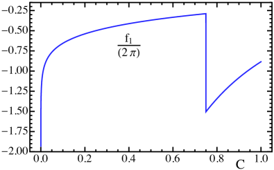
Figure 2: 𝒪(αs)𝒪subscript𝛼𝑠\mathcal{O}(\alpha_{s}) nonsingular C-parameter distribution, corresponding to Eq. (V).
Refer to caption
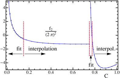
Figure 3: 𝒪(αs2)𝒪superscriptsubscript𝛼𝑠2\mathcal{O}(\alpha_{s}^{2}) nonsingular C-parameter distribution. The solid line shows our reconstruction, whereas dots with error bars correspond to the EVENT2 output with the singular terms subtracted. Our reconstruction consists of fit functions to the left of the red dashed line at C=0.15𝐶0.15C=0.15 and between the two red dashed lines at C=0.75𝐶0.75C=0.75 and C=0.8𝐶0.8C=0.8 and interpolation functions elsewhere.
Refer to caption
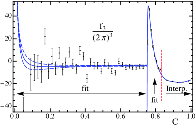
Figure 4: 𝒪(αs3)𝒪superscriptsubscript𝛼𝑠3\mathcal{O}(\alpha_{s}^{3}) nonsingular C-parameter distribution. The solid line shows our reconstruction, whereas dots with error bars correspond to the EERAD3 output with the singular terms subtracted. Our reconstruction consists of two fit functions, one for C<0.75𝐶0.75C<0.75 and another one for 0.75<C<0.8350.75𝐶0.8350.75<C<0.835, and an interpolation for C>0.835𝐶0.835C>0.835 (to the right of the red dashed vertical line).

At one loop, we can write down the exact form of the full distribution as a two-dimensional integral Ellis et al. (1980)

1σ0|dσ^dC|1loop=1subscript𝜎0superscriptd^𝜎d𝐶1loopabsent\displaystyle\frac{1}{\sigma_{0}}\bigg{|}\frac{\mathrm{d}\hat{\sigma}}{\mathrm{d}C}\bigg{|}^{\rm 1-loop}\,= (32)
αs2πCF01dx101dx2θ(x1+x21)x12+x22(1x1)(1x2)subscript𝛼𝑠2𝜋subscript𝐶𝐹superscriptsubscript01differential-dsubscript𝑥1superscriptsubscript01differential-dsubscript𝑥2𝜃subscript𝑥1subscript𝑥21superscriptsubscript𝑥12superscriptsubscript𝑥221subscript𝑥11subscript𝑥2\displaystyle\frac{\alpha_{s}}{2\pi}\,C_{F}\!\!\int_{0}^{1}\!\mathrm{d}x_{1}\!\int_{0}^{1}\!\mathrm{d}x_{2}\,\theta(x_{1}+x_{2}-1)\,\frac{x_{1}^{2}+x_{2}^{2}}{(1-x_{1})(1-x_{2})}
×δ(C6(1x1)(1x2)(x1+x21)x1x2(2x1x2)),absent𝛿𝐶61subscript𝑥11subscript𝑥2subscript𝑥1subscript𝑥21subscript𝑥1subscript𝑥22subscript𝑥1subscript𝑥2\displaystyle\times\delta\!\left(\!C-\frac{6\,(1-x_{1})(1-x_{2})(x_{1}+x_{2}-1)}{x_{1}x_{2}(2-x_{1}-x_{2})}\right),

which has support for 0<C<3/40𝐶340<C<3/4 and jumps to zero for C>3/4𝐶34C>3/4. After resolving the delta function, it becomes a one-dimensional integral that can be easily evaluated numerically. After subtracting off the one-loop singular piece discussed in Sec. IV, we obtain the result for f1subscript𝑓1f_{1} shown in Fig. 2. For C>3/4𝐶34C>3/4 the nonsingular distribution at this order is simply given by the negative of the singular, and for practical purposes one can find a parametrization for f1subscript𝑓1f_{1} for C<3/4𝐶34C<3/4, so we use

f1(C<0.75)= 2.25168+0.506802C+ 0.184585C2subscript𝑓1𝐶0.752.251680.506802𝐶0.184585superscript𝐶2\displaystyle f_{1}(C<0.75)\,=\,-\,2.25168+0.506802\,C\,+\,0.184585\,C^{2}
+ 0.121051C3+(0.8904760.544484C\displaystyle+\,0.121051\,C^{3}\,+(0.890476-0.544484\,C
 0.252937C20.0327797C3)ln(C),\displaystyle-\,0.252937\,C^{2}-0.0327797\,C^{3})\ln(C)\,,
f1(C>0.75)=43C[3+4ln(C6)].subscript𝑓1𝐶0.7543𝐶delimited-[]34𝐶6\displaystyle f_{1}(C>0.75)\,=\,\frac{4}{3C}\bigg{[}3+4\ln\bigg{(}\frac{C}{6}\bigg{)}\bigg{]}. (33)

For an average over C𝐶C, this result for f1(C)subscript𝑓1𝐶f_{1}(C) is accurate to 107superscript10710^{-7} and at worst for a particular C𝐶C is accurate at 105superscript10510^{-5}. An exact closed form in terms of elliptic functions for the integral in Eq. (32) has been found in Ref. Gardi and Magnea (2003).

The full 𝒪(αs2)𝒪superscriptsubscript𝛼𝑠2\mathcal{O}(\alpha_{s}^{2}) and 𝒪(αs3)𝒪superscriptsubscript𝛼𝑠3\mathcal{O}(\alpha_{s}^{3}) fixed-order distributions can be obtained numerically from the Fortran programs EVENT2 Catani and Seymour (1996, 1997) and EERAD3 Gehrmann-De Ridder et al. (2009); Gehrmann-De Ridder et al. (2014), respectively. At 𝒪(αs2)𝒪superscriptsubscript𝛼𝑠2\mathcal{O}(\alpha_{s}^{2}) we use log-binning EVENT2 results for C<0.2𝐶0.2C<0.2 and linear-binning (with bin size of 0.02) results for 0.2<C<0.750.2𝐶0.750.2<C<0.75. We then have additional log binning from 0.75<C<0.7750.75𝐶0.7750.75<C<0.775 (using bins in ln[C0.75]𝐶0.75\ln[C-0.75]) before returning to linear binning for C>0.775𝐶0.775C>0.775. We used runs with a total of 3×10113superscript10113\times 10^{11} events and an infrared cutoff y0=108subscript𝑦0superscript108y_{0}=10^{-8}. In the regions of linear binning, the statistical uncertainties are quite low and we can use a numerical interpolation for f2(C)subscript𝑓2𝐶f_{2}(C). For C<0.15𝐶0.15C<0.15 we use the ansatz, f2(C)=i=03ailniC+a4ClnCsubscript𝑓2𝐶superscriptsubscript𝑖03subscript𝑎𝑖superscript𝑖𝐶subscript𝑎4𝐶𝐶f_{2}(C)=\sum_{i=0}^{3}a_{i}\ln^{i}C+a_{4}\,C\ln C and fit the coefficients from EVENT2 output, including the constraint that the total fixed-order cross section gives the known 𝒪(αs2)𝒪superscriptsubscript𝛼𝑠2\mathcal{O}(\alpha_{s}^{2}) coefficient for the total cross section. The resulting values for the aisubscript𝑎𝑖a_{i} are given as functions of s2C~superscriptsubscript𝑠2~𝐶s_{2}^{\widetilde{C}}, the non-logarithmic coefficient in the partonic soft function. Details on the determination of this fit function and the determination of s2C~superscriptsubscript𝑠2~𝐶s_{2}^{\widetilde{C}} can be found below in Sec. VI. We find

s2C~= 43.2± 1.0,superscriptsubscript𝑠2~𝐶plus-or-minus43.21.0\displaystyle s_{2}^{\widetilde{C}}=-\,43.2\,\pm\,1.0\,, (34)

whose central value is used in Figs. 3, 4, 5, and 11, and whose uncertainty is included in our uncertainty analysis. For 0.75<C<0.80.75𝐶0.80.75<C<0.8 we employ another ansatz, f2(C)=i=01k=02bik(C0.75)ilnk[ 8(C0.75)/3]subscript𝑓2𝐶superscriptsubscript𝑖01superscriptsubscript𝑘02subscript𝑏𝑖𝑘superscript𝐶0.75𝑖superscript𝑘8𝐶0.753f_{2}(C)\,=\,\sum_{i=0}^{1}\sum_{k=0}^{2}b_{ik}\,(C-0.75)^{i}\ln^{k}[\,8\,(C-0.75)/3]. We use the values calculated in Ref. Catani and Webber (1997), b01=59.8728subscript𝑏0159.8728b_{01}=59.8728, b02=43.3122subscript𝑏0243.3122b_{02}=43.3122, and b12= 115.499subscript𝑏12115.499b_{12}=-\,115.499 and fit the rest of the coefficients to EVENT2 output. The final result for the two-loop nonsingular cross section coefficient then has the form

f2(C)+ϵ2lowδ2low(C)+ϵ2highδ2high(C).subscript𝑓2𝐶subscriptsuperscriptitalic-ϵlow2subscriptsuperscript𝛿low2𝐶subscriptsuperscriptitalic-ϵhigh2subscriptsuperscript𝛿high2𝐶\displaystyle f_{2}(C)\,+\,\epsilon^{\text{low}}_{2}\,\delta^{\text{low}}_{2}(C)\,+\,\epsilon^{\text{high}}_{2}\,\delta^{\text{high}}_{2}(C)\,. (35)

Here f2(C)subscript𝑓2𝐶f_{2}(C) gives the best fit in all regions, and δ2lowsuperscriptsubscript𝛿2low\delta_{2}^{\text{low}} and δ2highsuperscriptsubscript𝛿2high\delta_{2}^{\text{high}} give the 111-σ𝜎\sigma error functions for the lower fit (C<0.75𝐶0.75C<0.75) and upper fit (C>0.75𝐶0.75C>0.75), respectively. The two variables ϵ2lowsubscriptsuperscriptitalic-ϵlow2\epsilon^{\text{low}}_{2} and ϵ2highsubscriptsuperscriptitalic-ϵhigh2\epsilon^{\text{high}}_{2} are varied during our theory scans in order to account for the error in the nonsingular function. In Fig. 3, we show the EVENT2 data as dots and the best-fit nonsingular function as a solid blue line. The uncertainties are almost invisible on the scale of this plot.

In order to determine the 𝒪(αs3)𝒪superscriptsubscript𝛼𝑠3\mathcal{O}(\alpha_{s}^{3}) nonsingular cross section f3(C)subscript𝑓3𝐶f_{3}(C), we follow a similar procedure. The EERAD3 numerical output is based on an infrared cutoff y0=105subscript𝑦0superscript105y_{0}=10^{-5} and calculated with 6×1076superscript1076\times 10^{7} events for the three leading color structures and 107superscript10710^{7} events for the three subleading color structures. The results are linearly binned with a bin size of 0.02 for C<0.835𝐶0.835C<0.835 and a bin size of 0.010.010.01 for C>0.835𝐶0.835C>0.835. As the three-loop numerical results have larger uncertainties than the two-loop results, we employ a fit for all C<0.835𝐶0.835C<0.835 and use interpolation only above that value. The fit is split into two parts for C𝐶C below and above 0.750.750.75. For the lower fit, we use the ansatz f3(C)=i=15ailni(C)subscript𝑓3𝐶superscriptsubscript𝑖15subscript𝑎𝑖superscript𝑖𝐶f_{3}(C)=\sum_{i=1}^{5}a_{i}\ln^{i}(C). The results for the aisubscript𝑎𝑖a_{i} depend on the 𝒪(αs2)𝒪superscriptsubscript𝛼𝑠2\mathcal{O}(\alpha_{s}^{2}) partonic soft function coefficient s2C~superscriptsubscript𝑠2~𝐶s_{2}^{\widetilde{C}} and a combination of the three-loop coefficients in the partonic soft and jet function, s3C~+ 2j3superscriptsubscript𝑠3~𝐶2subscript𝑗3s_{3}^{\widetilde{C}}\,+\,2\,j_{3}. Due to the amount of numerical uncertainty in the EERAD3 results, it is not feasible to fit for this combination, so each of these parameters is left as a variable that is separately varied in our theory scans. Above C=0.75𝐶0.75C=0.75 we carry out a second fit, using the fit form f3(C)=i=04bilni(C0.75)subscript𝑓3𝐶superscriptsubscript𝑖04subscript𝑏𝑖superscript𝑖𝐶0.75f_{3}(C)=\sum_{i=0}^{4}b_{i}\ln^{i}(C-0.75). We use the value b4=122.718subscript𝑏4122.718b_{4}=122.718 predicted by exponentiation in Ref. Catani and Webber (1997). The rest of the b𝑏b’s depend on s2C~superscriptsubscript𝑠2~𝐶s_{2}^{\widetilde{C}}. The final result for the three-loop nonsingular cross section coefficient can once again be written in the form

f3(C)+ϵ3lowδ3low(C)+ϵ3highδ3high(C),subscript𝑓3𝐶subscriptsuperscriptitalic-ϵlow3superscriptsubscript𝛿3low𝐶subscriptsuperscriptitalic-ϵhigh3subscriptsuperscript𝛿high3𝐶\displaystyle f_{3}(C)+\epsilon^{\text{low}}_{3}\delta_{3}^{\text{low}}(C)+\epsilon^{\text{high}}_{3}\delta^{\text{high}}_{3}(C)\,, (36)

where f3(C)subscript𝑓3𝐶f_{3}(C) is the best-fit function and the δ3subscript𝛿3\delta_{3}’s give the 111-σ𝜎\sigma error function for the low (C<0.75𝐶0.75C<0.75) and high (C>0.75𝐶0.75C>0.75) fits. Exactly like for the 𝒪(αs2)𝒪superscriptsubscript𝛼𝑠2\mathcal{O}(\alpha_{s}^{2}) case, the ϵ3subscriptitalic-ϵ3\epsilon_{3}’s are varied in the final error analysis. In Fig. 4, we plot the EERAD3 data as dots, the best-fit function f3subscript𝑓3f_{3} as a solid line, and the nonsingular results with ϵ3low=ϵ3high=± 1subscriptsuperscriptitalic-ϵlow3subscriptsuperscriptitalic-ϵhigh3plus-or-minus1\epsilon^{\text{low}}_{3}=\epsilon^{\text{high}}_{3}=\pm\,1 as dashed lines. In this plot we take s2C~superscriptsubscript𝑠2~𝐶s_{2}^{\widetilde{C}} to its best-fit value and j3=s3C~=0subscript𝑗3superscriptsubscript𝑠3~𝐶0j_{3}=s_{3}^{\widetilde{C}}=0.

In the final error analysis, we vary the nonsingular parameters encoding the numerical extraction uncertainty ϵisubscriptitalic-ϵ𝑖\epsilon_{i}’s, as well as the profile parameter μnssubscript𝜇ns\mu_{\rm ns}. The uncertainties in our nonsingular fitting are obtained by taking ϵ2low,ϵ2high,ϵ3low,subscriptsuperscriptitalic-ϵlow2subscriptsuperscriptitalic-ϵhigh2subscriptsuperscriptitalic-ϵlow3\epsilon^{\rm low}_{2},\,\epsilon^{\text{high}}_{2},\,\epsilon^{\text{low}}_{3}, and ϵ3highsubscriptsuperscriptitalic-ϵhigh3\epsilon^{\text{high}}_{3} to be  11-\,1, 00, and 111 independently. The effects of ϵ2lowsubscriptsuperscriptitalic-ϵlow2\epsilon^{\text{low}}_{2}, ϵ2highsubscriptsuperscriptitalic-ϵhigh2\epsilon^{\text{high}}_{2} and ϵ3highsubscriptsuperscriptitalic-ϵhigh3\epsilon^{\text{high}}_{3} are essentially negligible in the tail region. Due to the high noise in the EERAD3 results, the variation of ϵ3highsubscriptsuperscriptitalic-ϵhigh3\epsilon^{\text{high}}_{3} is not negligible in the tail region, but because it comes in at 𝒪(αs3)𝒪superscriptsubscript𝛼𝑠3{\cal O}(\alpha_{s}^{3}), it is still small. We vary the nonsingular renormalization scale μnssubscript𝜇ns\mu_{\rm ns} in a way described in Sec. VIII.

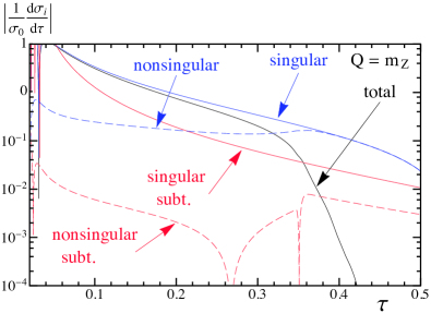
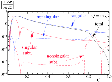
In order to have an idea about the size of the nonsingular distributions with respect to the singular terms, we quote numbers for the average value of the one-, two-, and three-loop distributions between C=0.2𝐶0.2C=0.2 and C=0.6𝐶0.6C=0.6: 5,21,76521765,21,76 (singular at one, two, and three loops);  0.4, 1, 40.414-\,0.4,-\,1,-\,4 (nonsingular at one, two, and three loops). Hence, in the region to be used for fitting αs(mZ)subscript𝛼𝑠subscript𝑚𝑍\alpha_{s}(m_{Z}), the singular distribution is 121212 (at 1-loop) to 202020 (at two and three loops) times larger than the nonsingular one and has the opposite sign. Plots comparing the singular and nonsingular cross sections for all C𝐶C values are given below in Fig. 5.

VI Determination of Two-Loop Soft Function Parameters

In this section we will expand on the procedure used to extract the 𝒪(αs2)𝒪superscriptsubscript𝛼𝑠2\mathcal{O}(\alpha_{s}^{2}) non-logarithmic coefficient in the soft function using EVENT2. For a general event shape, we can separate the partonic cross section into a singular part where the cross section involves δ(e)𝛿𝑒\delta(e) or lnk(e)/esuperscript𝑘𝑒𝑒\ln^{k}(e)/e, 333The numerical outcome of a parton-level Monte Carlo such as EVENT2 contains only the power of logs, but the complete distributions can be obtained from knowledge of the SCET soft and jet functions. and a nonsingular part with integrable functions, that diverge at most as lnk(e)superscript𝑘𝑒\ln^{k}(e). Of course, when these are added together and integrated over the whole spectrum of the event shape distribution, we get the correct fixed-order normalization:

σ^had=0emaxde(dσ^sde+dσ^nsde).subscript^𝜎hadsuperscriptsubscript0subscript𝑒maxdifferential-d𝑒dsubscript^𝜎sd𝑒dsubscript^𝜎nsd𝑒\hat{\sigma}_{\rm had}=\int_{0}^{e_{\rm max}}\!\mathrm{d}e\left(\frac{\mathrm{d}\hat{\sigma}_{\rm s}}{\mathrm{d}e}+\frac{\mathrm{d}\hat{\sigma}_{\rm ns}}{\mathrm{d}e}\right). (37)

Here emaxsubscript𝑒maxe_{\text{max}} is the maximum value for the given event shape (for C-parameter, emax=1subscript𝑒max1e_{\text{max}}=1). Using SCET, we can calculate the singular cross section at 𝒪(αs2)𝒪superscriptsubscript𝛼𝑠2\mathcal{O}(\alpha_{s}^{2}), having the form

1σ0dσ^s(2)de=Aδδ(e)+n=03Dn[lnnee]+.1subscript𝜎0dsuperscriptsubscript^𝜎s2d𝑒subscript𝐴𝛿𝛿𝑒superscriptsubscript𝑛03subscript𝐷𝑛subscriptdelimited-[]superscript𝑛𝑒𝑒\dfrac{1}{\sigma_{0}}\frac{\mathrm{d}\hat{\sigma}_{\rm s}^{(2)}}{\mathrm{d}e}=A_{\delta}\,\delta(e)+\sum_{n=0}^{3}\,D_{n}\bigg{[}\frac{\ln^{n}e}{e}\bigg{]}_{+}\,. (38)

To define dσ^s(2)/dedsuperscriptsubscript^𝜎s2d𝑒\mathrm{d}\hat{\sigma}_{\rm s}^{(2)}/\mathrm{d}e we factor out αs2/16π2superscriptsubscript𝛼𝑠216superscript𝜋2\alpha_{s}^{2}/16\pi^{2} and set μ=Q𝜇𝑄\mu=Q. The only unknown term at 𝒪(αs2)𝒪superscriptsubscript𝛼𝑠2{\cal O}(\alpha_{s}^{2}) for the C-parameter distribution is the two-loop constant s2C~superscriptsubscript𝑠2~𝐶s_{2}^{\widetilde{C}} in the soft function, which contributes to Aδsubscript𝐴𝛿A_{\delta}. The explicit result for the terms in Eq. (38) can be obtained from H(Q,μ)P(Q,QC/6,μ)𝐻𝑄𝜇𝑃𝑄𝑄𝐶6𝜇H(Q,\mu)\,P(Q,QC/6,\mu) which are given in App. A. This allows us to write the singular integral in (37) as a function of s2C~superscriptsubscript𝑠2~𝐶s_{2}^{\widetilde{C}} and known constants.

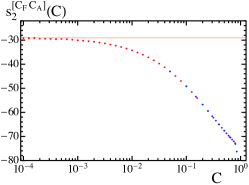
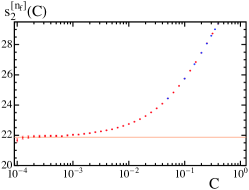
We extract the two-loop nonsingular portion of the cross section from EVENT2 data. Looking now at the specific case of C-parameter, we use both log-binning (in the small C𝐶C region, which is then described with high accuracy) and linear binning (for the rest). By default we use logarithmic binning for C<Cfit=0.2𝐶subscript𝐶fit0.2C<C_{\rm fit}=0.2, but this boundary is changed between 0.150.150.15 and 0.250.250.25 in order to estimate systematic uncertainties of our method. In the logarithmically binned region we use a fit function to extrapolate for the full behavior of the nonsingular cross section. In order to determine the coefficients of the fit function we use data between Ccutsubscript𝐶cutC_{\rm cut} and Cfitsubscript𝐶fitC_{\rm fit}. By default we take the value Ccut=104subscript𝐶cutsuperscript104C_{\rm cut}=10^{-4}, but we also explore different values between 5×1055superscript1055\times 10^{-5} and 7.625×1047.625superscript1047.625\times 10^{-4} to estimate systematic uncertainties. We employ the following functional form, motivated by the expected nonsingular logarithms

1σ0dσ^fitnsdC=i=03ailniC+a4ClnnC,1subscript𝜎0dsubscriptsuperscript^𝜎nsfitd𝐶superscriptsubscript𝑖03subscript𝑎𝑖superscript𝑖𝐶subscript𝑎4𝐶superscript𝑛𝐶\displaystyle\dfrac{1}{\sigma_{0}}\frac{\mathrm{d}\hat{\sigma}^{\rm ns}_{\rm fit}}{\mathrm{d}C}=\sum_{i=0}^{3}\,a_{i}\,\ln^{i}C+a_{4}\,C\ln^{n}C\,, (39)

taking the value n=1𝑛1n=1 as default and exploring values 0n30𝑛30\leq n\leq 3 as an additional source of systematic uncertainty.

For the region with linear binning, we can simply calculate the relevant integrals by summing over the bins. One can also sum bins that contain the shoulder region as its singular behavior is integrable. These various pieces all combine into a final formula that can be used to extract the two-loop constant piece of the soft function:

σ^had(2)=01dCdσ^s(2)dC+0CfitdCdσ^fitnsdC+Cfit1dCdσ^intnsdC.superscriptsubscript^𝜎had2superscriptsubscript01differential-d𝐶dsubscriptsuperscript^𝜎2sd𝐶superscriptsubscript0subscript𝐶fitdifferential-d𝐶dsubscriptsuperscript^𝜎nsfitd𝐶superscriptsubscriptsubscript𝐶fit1differential-d𝐶dsubscriptsuperscript^𝜎nsintd𝐶\displaystyle\hat{\sigma}_{\rm had}^{(2)}=\!\int_{0}^{1}\!\mathrm{d}C\,\frac{\mathrm{d}\hat{\sigma}^{(2)}_{\rm s}}{\mathrm{d}C}\,+\!\int_{0}^{C_{\rm fit}}\!\!\mathrm{d}C\,\frac{\mathrm{d}\hat{\sigma}^{\rm ns}_{\rm fit}}{\mathrm{d}C}\,+\!\int_{C_{\rm fit}}^{1}\!\!\mathrm{d}C\,\frac{\mathrm{d}\hat{\sigma}^{\text{ns}}_{\rm int}}{\mathrm{d}C}. (40)

Using Eq. (40) one can extract s2C~superscriptsubscript𝑠2~𝐶s_{2}^{\widetilde{C}}, which can be decomposed into its various color components as

s2C~=CF2s2[CF2]+CFCAs2[CFCA]+CFnfTFs2[nf].superscriptsubscript𝑠2~𝐶superscriptsubscript𝐶𝐹2superscriptsubscript𝑠2delimited-[]superscriptsubscript𝐶𝐹2subscript𝐶𝐹subscript𝐶𝐴superscriptsubscript𝑠2delimited-[]subscript𝐶𝐹subscript𝐶𝐴subscript𝐶𝐹subscript𝑛𝑓subscript𝑇𝐹superscriptsubscript𝑠2delimited-[]subscript𝑛𝑓\displaystyle s_{2}^{\widetilde{C}}=C_{F}^{2}\,s_{2}^{[C_{F}^{2}]}+C_{F}\,C_{A}s_{2}^{[C_{F}C_{A}]}+C_{F}\,n_{f}T_{F}s_{2}^{[n_{f}]}\,. (41)

The results of this extraction are

s2[CF2]superscriptsubscript𝑠2delimited-[]superscriptsubscript𝐶𝐹2\displaystyle s_{2}^{[C_{F}^{2}]} =  0.46±0.75,absentplus-or-minus0.460.75\displaystyle=\,-\,\,0.46\,\pm 0.75\,,
s2[CFCA]superscriptsubscript𝑠2delimited-[]subscript𝐶𝐹subscript𝐶𝐴\displaystyle s_{2}^{[C_{F}C_{A}]} = 29.08±0.13,absentplus-or-minus29.080.13\displaystyle=-\,29.08\pm 0.13\,, (42)
s2[nf]superscriptsubscript𝑠2delimited-[]subscript𝑛𝑓\displaystyle s_{2}^{[n_{f}]} = 21.87±0.03.absentplus-or-minus21.870.03\displaystyle=~{}~{}\>21.87\pm 0.03\,.

The quoted uncertainties include a statistical component coming from the fitting procedure and a systematical component coming from the parameter variations explained above, added in quadrature. Note that the value for s2[CF2]superscriptsubscript𝑠2delimited-[]superscriptsubscript𝐶𝐹2s_{2}^{[C_{F}^{2}]} is consistent with zero, as expected from exponentiation Hoang and Kluth (2008). For our analysis we will always take s2[CF2]=0superscriptsubscript𝑠2delimited-[]superscriptsubscript𝐶𝐹20s_{2}^{[C_{F}^{2}]}=0. We have cross-checked that, when a similar extraction is repeated for the case of thrust, the extracted values are consistent with those calculated analytically in Refs. Kelley et al. (2011); Monni et al. (2011). This indicates a high level of accuracy in the fitting procedure. We have also confirmed that following the alternate fit procedure of Ref. Hoang and Kluth (2008) gives compatible results, as shown in App. B.

VII Power Corrections and Renormalon-Free Scheme

The expressions for the theoretical prediction of the C-parameter distribution in the dijet region shown in Eqs. (26) and (27) incorporate that the full soft function can be written as a convolution of the partonic soft function S^Csubscript^𝑆𝐶\hat{S}_{C} and the nonperturbative shape function FCsubscript𝐹𝐶F_{C}Hoang and Stewart (2008)444Here we use the relations S^C(,μ)=S^C~(/6,μ)/6subscript^𝑆𝐶𝜇subscript^𝑆~𝐶6𝜇6\hat{S}_{C}(\ell,\mu)=\hat{S}_{\widetilde{C}}(\ell/6,\mu)/6 and FC()=FC~(/6)/6subscript𝐹𝐶subscript𝐹~𝐶66F_{C}(\ell)=F_{\widetilde{C}}(\ell/6)/6. :

SC(k,μ)=dkS^C(kk,μ)FC(k,ΔC).subscript𝑆𝐶𝑘𝜇differential-dsuperscript𝑘subscript^𝑆𝐶𝑘superscript𝑘𝜇subscript𝐹𝐶superscript𝑘subscriptΔ𝐶\displaystyle S_{C}(k,\mu)=\!\int\!\mathrm{d}k^{\prime}\,\hat{S}_{C}(k-k^{\prime},\mu)F_{C}(k^{\prime},\Delta_{C})\,. (43)

Here, the partonic soft function S^Csubscript^𝑆𝐶\hat{S}_{C} is defined in fixed order in MS¯¯MS\overline{\text{MS}}. The shape function FCsubscript𝐹𝐶F_{C} allows a smooth transition between the peak and tail regions, where different kinematic expansions are valid, and ΔCsubscriptΔ𝐶\Delta_{C} is a parameter of the shape function that represents an offset from zero momentum and that will be discussed further below. By definition, the shape function satisfies the relations FC(k,ΔC)=FC(k2ΔC)subscript𝐹𝐶𝑘subscriptΔ𝐶subscript𝐹𝐶𝑘2subscriptΔ𝐶F_{C}(k,\Delta_{C})=F_{C}(k-2\Delta_{C}) and FC(k<0)=0subscript𝐹𝐶𝑘00F_{C}(k<0)=0. In the tail region, where QC/6ΛQCDmuch-greater-than𝑄𝐶6subscriptΛQCDQC/6\gg\Lambda_{\text{QCD}}, this soft function can be expanded to give

SC(k,μ)=S^C(k)dS^C(k)dkΩ¯1C+𝒪(αsΛQCDQC,ΛQCD2Q2C2),subscript𝑆𝐶𝑘𝜇subscript^𝑆𝐶𝑘dsubscript^𝑆𝐶𝑘d𝑘superscriptsubscript¯Ω1𝐶𝒪subscript𝛼𝑠subscriptΛQCD𝑄𝐶superscriptsubscriptΛQCD2superscript𝑄2superscript𝐶2\displaystyle S_{C}(k,\mu)=\hat{S}_{C}(k)-\frac{\mathrm{d}\hat{S}_{C}(k)}{\mathrm{d}k}\,\overline{\Omega}_{1}^{C}+{\cal O}\Big{(}\frac{\alpha_{s}\Lambda_{\rm QCD}}{QC},\frac{\Lambda_{\rm QCD}^{2}}{Q^{2}C^{2}}\Big{)}, (44)

where Ω¯1Csuperscriptsubscript¯Ω1𝐶\overline{\Omega}_{1}^{C} is the leading nonperturbative power correction in MS¯¯MS\overline{\rm MS} which effectively introduces a shift of the distribution in the tail region Abbate et al. (2011). The Ω¯1Csuperscriptsubscript¯Ω1𝐶\overline{\Omega}_{1}^{C} power correction

Ω¯1C(μ)superscriptsubscript¯Ω1𝐶𝜇\displaystyle\overline{\Omega}_{1}^{C}(\mu) =1Nc0|trY¯n¯TYn(QC^)YnY¯n¯|0,absent1subscript𝑁𝑐quantum-operator-product0trsuperscriptsubscript¯𝑌¯𝑛𝑇subscript𝑌𝑛𝑄^𝐶superscriptsubscript𝑌𝑛superscriptsubscript¯𝑌¯𝑛0\displaystyle=\frac{1}{N_{c}}\big{\langle}0\big{|}{\rm tr}\>\overline{Y}_{\bar{n}}^{T}Y_{n}(Q\widehat{C})Y_{n}^{\dagger}\overline{Y}_{\bar{n}}^{*}\big{|}0\big{\rangle}\,, (45)

is related to Ω¯1τsuperscriptsubscript¯Ω1𝜏\overline{\Omega}_{1}^{\tau}, the first moment of the thrust shape function, as given in Eq. (2). In addition to the normalization difference that involves a factor of 3π/23𝜋23\pi/2, their relation is further affected by hadron-mass effects which cause an additional deviation at the 2.5% level (computed in Sec. VII.1). The dominant contributions of the 𝒪(αsΛQCD/QC)𝒪subscript𝛼𝑠subscriptΛQCD𝑄𝐶{\cal O}(\alpha_{s}\Lambda_{\rm QCD}/QC) corrections indicated in Eq. (44) are log enhanced and will be captured once we include the μ𝜇\mu-anomalous dimension for Ω1CsuperscriptsubscriptΩ1𝐶\Omega_{1}^{C} that is induced by hadron-mass effects Mateu et al. (2013). There are additional 𝒪(αsΛQCD/QC)𝒪subscript𝛼𝑠subscriptΛQCD𝑄𝐶{\cal O}(\alpha_{s}\Lambda_{\rm QCD}/QC) corrections, which we neglect, that do not induce a shift. We consider hadron-mass effects in detail in Sec. VII.1.

From Eq. (43) and the OPE of Eq. (44), we can immediately read off the relations

dkkFC(k,ΔC)=2ΔC+dkkFC(k)=Ω¯1C,differential-dsuperscript𝑘superscript𝑘subscript𝐹𝐶superscript𝑘subscriptΔ𝐶2subscriptΔ𝐶differential-dsuperscript𝑘superscript𝑘subscript𝐹𝐶superscript𝑘superscriptsubscript¯Ω1𝐶\displaystyle\!\int\!\mathrm{d}k^{\prime}k^{\prime}F_{C}(k^{\prime},\Delta_{C})=2\,\Delta_{C}+\!\int\!\mathrm{d}k^{\prime}k^{\prime}F_{C}(k^{\prime})=\overline{\Omega}_{1}^{C}\,,
dkFC(k)=1,differential-dsuperscript𝑘subscript𝐹𝐶superscript𝑘1\displaystyle\!\int\!\mathrm{d}k^{\prime}F_{C}(k^{\prime})=1\,, (46)

which state that the first moment of the shape function provides the leading power correction and that the shape function is normalized. In the peak, it is no longer sufficient to keep only the first moment, as there is no OPE when QC/6ΛQCDsimilar-to𝑄𝐶6subscriptΛQCDQC/6\sim\Lambda_{\text{QCD}} and we must keep the full dependence on the model function in Eq. (43).

The partonic soft function in MS¯¯MS\overline{\text{MS}} has an 𝒪(ΛQCD)𝒪subscriptΛQCD\mathcal{O}(\Lambda_{\rm QCD}) renormalon, an ambiguity which is related to a linear sensitivity in its perturbative series. This renormalon ambiguity is in turn inherited to the numerical values for Ω¯1Csuperscriptsubscript¯Ω1𝐶\overline{\Omega}_{1}^{C} obtained in fits to the experimental data. It is possible to avoid this renormalon issue by switching to a different scheme for Ω1CsuperscriptsubscriptΩ1𝐶\Omega_{1}^{C}, which involves subtractions in the partonic soft function that remove this type of infrared sensitivity. Following the results of Ref. Hoang and Stewart (2008), we write ΔCsubscriptΔ𝐶\Delta_{C} as

ΔCsubscriptΔ𝐶\displaystyle\Delta_{C} =3π2[Δ¯(R,μ)+δ(R,μ)].absent3𝜋2delimited-[]¯Δ𝑅𝜇𝛿𝑅𝜇\displaystyle=\frac{3\pi}{2}[\,\bar{\Delta}(R,\mu)+\delta(R,\mu)\,]\,. (47)

The term δ(R,μ)𝛿𝑅𝜇\delta(R,\mu) is a perturbative series in αs(μ)subscript𝛼𝑠𝜇\alpha_{s}(\mu) which has the same renormalon behavior as Ω¯1Csuperscriptsubscript¯Ω1𝐶\overline{\Omega}_{1}^{C}. In the factorization formula, it is grouped into the partonic soft function S^Csubscript^𝑆𝐶\hat{S}_{C} through the exponential factor involving δ(R,μ)𝛿𝑅𝜇\delta(R,\mu) shown in Eq. (29). Upon simultaneous perturbative expansion of the exponential together with S^Csubscript^𝑆𝐶\hat{S}_{C}, the 𝒪(ΛQCD)𝒪subscriptΛQCD\mathcal{O}(\Lambda_{\rm QCD}) renormalon is subtracted. The term Δ¯(R,μ)¯Δ𝑅𝜇\bar{\Delta}(R,\mu) then becomes a nonperturbative parameter which is free of the 𝒪(ΛQCD)𝒪subscriptΛQCD\mathcal{O}(\Lambda_{\rm QCD}) renormalon. Its dependence on the subtraction scale R𝑅R and on μ𝜇\mu is dictated by δ(R,μ)𝛿𝑅𝜇\delta(R,\mu) since ΔCsubscriptΔ𝐶\Delta_{C} is R𝑅R and μ𝜇\mu independent. The subtraction scale R𝑅R encodes the momentum scale associated with the removal of the linearly infrared-sensitive fluctuations. The factor 3π/23𝜋23\pi/2 is a normalization coefficient that relates the 𝒪(ΛQCD)𝒪subscriptΛQCD{\cal O}(\Lambda_{\rm QCD}) renormalon ambiguity of the C𝐶C soft function SCsubscript𝑆𝐶S_{C} to the one for the thrust soft function. Taking into account this normalization we can use for δ(R,μ)𝛿𝑅𝜇\delta(R,\mu) the scheme for the thrust soft function already defined in Ref. Abbate et al. (2011),

δ(R,μ)=R2eγEddln(ix)[lnSτpart(x,μ)]x=(iReγE)1,𝛿𝑅𝜇𝑅2superscript𝑒subscript𝛾𝐸dd𝑖𝑥subscriptdelimited-[]subscriptsuperscript𝑆part𝜏𝑥𝜇𝑥superscript𝑖𝑅superscript𝑒subscript𝛾𝐸1\!\!\!\!\delta(R,\mu)=\frac{R}{2}\,e^{\gamma_{E}}\frac{\mathrm{d}}{\mathrm{d}\ln(ix)}\big{[}\ln S^{\text{part}}_{\tau}(x,\mu)\big{]}_{x=(iRe^{\gamma_{E}})^{-1}}, (48)

where Sτpart(x,μ)subscriptsuperscript𝑆part𝜏𝑥𝜇S^{\text{part}}_{\tau}(x,\mu) is the position-space thrust partonic soft function. From this, we find that the perturbative series for the subtraction is

δ(R,μ)=ReγEi=1αsi(μ)δi(R,μ).𝛿𝑅𝜇𝑅superscript𝑒subscript𝛾𝐸superscriptsubscript𝑖1superscriptsubscript𝛼𝑠𝑖𝜇superscript𝛿𝑖𝑅𝜇\displaystyle\delta(R,\mu)=R\,e^{\gamma_{E}}\!\sum_{i=1}^{\infty}\alpha_{s}^{i}(\mu)\,\delta^{i}(R,\mu)\,. (49)

Here the δi2subscript𝛿𝑖2\delta_{i\geq 2} depend on both the adjoint Casimir CA=3subscript𝐶𝐴3C_{A}=3 and the number of light flavors in combinations that are unrelated to the QCD beta function. Using five light flavors the first three coefficients have been calculated in Ref. Hoang and Kluth (2008) as

π2δ1(R,μ)𝜋2superscript𝛿1𝑅𝜇\displaystyle\frac{\pi}{2}\,\delta^{1}(R,\mu) = 1.33333LR,absent1.33333subscript𝐿𝑅\displaystyle=-\,1.33333\,L_{R}\,,
π2δ2(R,μ)𝜋2superscript𝛿2𝑅𝜇\displaystyle\frac{\pi}{2}\,\delta^{2}(R,\mu) = 0.2454820.732981LR0.813459LR2,absent0.2454820.732981subscript𝐿𝑅0.813459superscriptsubscript𝐿𝑅2\displaystyle=-\,0.245482-0.732981\,L_{R}-0.813459\,L_{R}^{2}\,,
π2δ3(R,μ)𝜋2superscript𝛿3𝑅𝜇\displaystyle\frac{\pi}{2}\,\delta^{3}(R,\mu) = 0.8686280.977769LRabsent0.8686280.977769subscript𝐿𝑅\displaystyle=-\,0.868628\,-0.977769\,L_{R}
1.22085LR20.661715LR3,1.22085superscriptsubscript𝐿𝑅20.661715superscriptsubscript𝐿𝑅3\displaystyle\quad-1.22085\,L_{R}^{2}-0.661715\,L_{R}^{3}\,, (50)

where LR=ln(μ/R)subscript𝐿𝑅𝜇𝑅L_{R}=\ln(\mu/R). Using these δ𝛿\delta’s, we can make a scheme change on the first moment to what we call the Rgap scheme:

Ω1C(R,μ)superscriptsubscriptΩ1𝐶𝑅𝜇\displaystyle\Omega_{1}^{C}(R,\mu) =Ω¯1C(μ)3πδ(R,μ).absentsuperscriptsubscript¯Ω1𝐶𝜇3𝜋𝛿𝑅𝜇\displaystyle=\overline{\Omega}_{1}^{C}(\mu)-3\pi\,\delta(R,\mu)\,. (51)

In contrast to the MS¯¯MS\overline{\text{MS}} scheme Ω¯1C(μ)superscriptsubscript¯Ω1𝐶𝜇\overline{\Omega}_{1}^{C}(\mu), the Rgap scheme Ω1C(R,μ)superscriptsubscriptΩ1𝐶𝑅𝜇\Omega_{1}^{C}(R,\mu) is free of the ΛQCDsubscriptΛQCD\Lambda_{\rm QCD} renormalon. From Eq. (VII) it is then easy to see that the first moment of the shape function becomes

dkkFC(k3πΔ¯(R,μ))=Ω1C(R,μ).differential-d𝑘𝑘subscript𝐹𝐶𝑘3𝜋¯Δ𝑅𝜇superscriptsubscriptΩ1𝐶𝑅𝜇\int\!\mathrm{d}k\,k\,F_{C}\big{(}k-3\pi\,\overline{\Delta}(R,\mu)\big{)}=\Omega_{1}^{C}(R,\mu)\,. (52)

The factorization in Eq. (43) can now be written as

SC(k,μ)subscript𝑆𝐶𝑘𝜇\displaystyle\!\!\!S_{C}(k,\mu) =dke 3πδ(R,μ)kS^C(kk,μ)absentdifferential-dsuperscript𝑘superscript𝑒3𝜋𝛿𝑅𝜇𝑘subscript^𝑆𝐶𝑘superscript𝑘𝜇\displaystyle=\!\int\!\mathrm{d}k^{\prime}\,e^{-\,3\pi\delta(R,\mu)\frac{\partial}{\partial k}}\hat{S}_{C}(k-k^{\prime},\mu)
×FC(k3πΔ¯(R,μ)).absentsubscript𝐹𝐶superscript𝑘3𝜋¯Δ𝑅𝜇\displaystyle\times F_{C}\big{(}k^{\prime}-3\pi\,\overline{\Delta}(R,\mu)\big{)}\,. (53)

The logs in Eq. (VII) can become large when μ𝜇\mu and R𝑅R are far apart. This imposes a constraint that Rμsimilar-to𝑅𝜇R\sim\mu, which will require the subtraction scale to depend on C𝐶C in a way similar to μ𝜇\mu. On the other hand, we also must consider the power counting Ω¯CΛQCDsimilar-tosuperscript¯Ω𝐶subscriptΛQCD\overline{\Omega}^{C}\sim\Lambda_{\text{QCD}}, which leads us to desire using R1similar-to-or-equals𝑅1R\simeq 1 GeV. In order to satisfy both of these constraints in the tail region, where μQC/61similar-to𝜇𝑄𝐶6much-greater-than1\mu\sim QC/6\gg 1 GeV, we (i) employ Rμsimilar-to𝑅𝜇R\sim\mu for the subtractions in δ(R,μ)𝛿𝑅𝜇\delta(R,\mu) that are part of the Rgap partonic soft function and (ii) use the R-evolution to relate the gap parameter Δ¯(R,μ)¯Δ𝑅𝜇\bar{\Delta}(R,\mu) to the reference gap parameter Δ¯(RΔ,μΔ)¯Δsubscript𝑅Δsubscript𝜇Δ\bar{\Delta}(R_{\Delta},\mu_{\Delta}) with RΔμΔ𝒪(1GeV)similar-tosubscript𝑅Δsubscript𝜇Δsimilar-to𝒪1GeVR_{\Delta}\sim\mu_{\Delta}\sim{\cal O}(1\,\text{GeV}) where the ΛQCDsubscriptΛQCD\Lambda_{\rm QCD} counting applies Hoang et al. (2008, 2010); Hoang and Kluth (2008). The formulae for the R𝑅R-RGE and μ𝜇\mu-RGE are

RddRΔ¯(R,R)𝑅dd𝑅¯Δ𝑅𝑅\displaystyle R\frac{\mathrm{d}}{\mathrm{d}R}\bar{\Delta}(R,R) =Rn=0γnR(αs(R)4π)n+1,absent𝑅superscriptsubscript𝑛0superscriptsubscript𝛾𝑛𝑅superscriptsubscript𝛼𝑠𝑅4𝜋𝑛1\displaystyle=-\,R\sum_{n=0}^{\infty}\gamma_{n}^{R}\left(\frac{\alpha_{s}(R)}{4\pi}\right)^{\!\!n+1},
μddμΔ¯(R,μ)𝜇dd𝜇¯Δ𝑅𝜇\displaystyle\mu\frac{\mathrm{d}}{\mathrm{d}\mu}\bar{\Delta}(R,\mu) =2ReγEn=0Γncusp(αs(μ)4π)n+1,absent2𝑅superscript𝑒subscript𝛾𝐸superscriptsubscript𝑛0superscriptsubscriptΓ𝑛cuspsuperscriptsubscript𝛼𝑠𝜇4𝜋𝑛1\displaystyle=2\,R\,e^{\gamma_{E}}\sum_{n=0}^{\infty}\Gamma_{n}^{\text{cusp}}\left(\frac{\alpha_{s}(\mu)}{4\pi}\right)^{\!\!n+1}, (54)

where for five flavors the ΓncuspsuperscriptsubscriptΓ𝑛cusp\Gamma_{n}^{\text{cusp}} is given in App. A and the γRsuperscript𝛾𝑅\gamma^{R} coefficients are given by

γ0Rsuperscriptsubscript𝛾0𝑅\displaystyle\gamma_{0}^{R} =0,γ1R= 43.954260,γ2R= 606.523329.formulae-sequenceabsent0formulae-sequencesuperscriptsubscript𝛾1𝑅43.954260superscriptsubscript𝛾2𝑅606.523329\displaystyle=0,\;\gamma_{1}^{R}=-\,43.954260\,,\;\gamma_{2}^{R}=-\,606.523329\,. (55)

The solution to Eq. (VII) is given, at NkLL, by

Δ¯(R,μ)¯Δ𝑅𝜇\displaystyle\bar{\Delta}(R,\mu) =Δ¯(RΔ,μΔ)+ReγEω[Γcusp,μ,R]absent¯Δsubscript𝑅Δsubscript𝜇Δ𝑅superscript𝑒subscript𝛾𝐸𝜔superscriptΓcusp𝜇𝑅\displaystyle=\bar{\Delta}(R_{\Delta},\mu_{\Delta})+R\,e^{\gamma_{E}}\omega\,[\,\Gamma^{\text{cusp}},\mu,R\,]
+RΔeγEω[Γcusp,RΔ,μΔ]subscript𝑅Δsuperscript𝑒subscript𝛾𝐸𝜔superscriptΓcuspsubscript𝑅Δsubscript𝜇Δ\displaystyle+R_{\Delta}e^{\gamma_{E}}\omega\,[\,\Gamma^{\text{cusp}},R_{\Delta},\mu_{\Delta}\,]
+ΛQCD(k)j=0k(1)jSjeiπb^1superscriptsubscriptΛQCD𝑘superscriptsubscript𝑗0𝑘superscript1𝑗subscript𝑆𝑗superscript𝑒𝑖𝜋subscript^𝑏1\displaystyle+\Lambda_{\text{QCD}}^{(k)}\,\sum_{j=0}^{k}(-1)^{j}S_{j}e^{i\pi\hat{b}_{1}}
×[Γ(b^1j,t1)Γ(b^1j,t0)]absentdelimited-[]Γsubscript^𝑏1𝑗subscript𝑡1Γsubscript^𝑏1𝑗subscript𝑡0\displaystyle\times\big{[}\,\Gamma(-\,\hat{b}_{1}-j,t_{1})-\Gamma(-\,\hat{b}_{1}-j,t_{0})\,\big{]}
Δ¯(RΔ,μΔ)+Δdiff(RΔ,R,μΔ,μ).absent¯Δsubscript𝑅Δsubscript𝜇ΔsuperscriptΔdiffsubscript𝑅Δ𝑅subscript𝜇Δ𝜇\displaystyle\equiv\bar{\Delta}(R_{\Delta},\mu_{\Delta})+\Delta^{\rm diff}(R_{\Delta},R,\mu_{\Delta},\mu)\,. (56)

For the convenience of the reader, the definition for ω𝜔\omega is provided in Eq. (A), and the values for b^1subscript^𝑏1\hat{b}_{1} and the Sjsubscript𝑆𝑗S_{j} are given in Eq. (E). In order to satisfy the power counting criterion for R𝑅R, we specify the parameter Δ¯(RΔ,μΔ)¯Δsubscript𝑅Δsubscript𝜇Δ\bar{\Delta}(R_{\Delta},\mu_{\Delta}) at the low reference scales RΔ=μΔ=2GeVsubscript𝑅Δsubscript𝜇Δ2GeVR_{\Delta}=\mu_{\Delta}=2\,\text{GeV}. We then use Eq. (VII) to evolve this parameter up to a scale R(C)𝑅𝐶R(C), which is given in Sec. VIII and satisfies the condition R(C)μS(C)similar-to𝑅𝐶subscript𝜇𝑆𝐶R(C)\sim\mu_{S}(C) in order to avoid large logs. This R-evolution equation yields a similar equation for the running of Ω1C(R,μS)superscriptsubscriptΩ1𝐶𝑅subscript𝜇𝑆\Omega_{1}^{C}(R,\mu_{S}), which is easily found from Eqs. (47) and (51).
Refer to caption
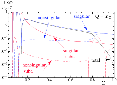
Figure 5: Singular and nonsingular components of the fixed-order C-parameter cross section, including up to 𝒪(αs3)𝒪superscriptsubscript𝛼𝑠3{\cal O}(\alpha_{s}^{3}) terms, with Ω1=0.25subscriptΩ10.25\Omega_{1}=0.25\,GeV and αs(mZ)=0.1141subscript𝛼𝑠subscript𝑚𝑍0.1141\alpha_{s}(m_{Z})=0.1141.

We also apply the Rgap scheme in the nonsingular part of the cross section by using the convolution

dke 3πδ(R,μs)QCdσ^nsdC(CkQ,μnsQ)differential-dsuperscript𝑘superscript𝑒3𝜋𝛿𝑅subscript𝜇𝑠𝑄𝐶dsubscript^𝜎nsd𝐶𝐶superscript𝑘𝑄subscript𝜇ns𝑄\displaystyle\!\!\!\int\!\mathrm{d}k^{\prime}\,e^{-\,3\pi\frac{\delta(R,\mu_{\!s})}{Q}\frac{\partial}{\partial C}}\frac{\mathrm{d}\hat{\sigma}_{\text{ns}}}{\mathrm{d}C}\Big{(}C-\frac{k^{\prime}}{Q},\frac{\mu_{\text{ns}}}{Q}\Big{)}
×FC(k3πΔ¯(R,μS)).absentsubscript𝐹𝐶superscript𝑘3𝜋¯Δ𝑅subscript𝜇𝑆\displaystyle\times F_{C}\big{(}k^{\prime}-3\pi\,\bar{\Delta}(R,\mu_{S})\big{)}\,. (57)

By employing the Rgap scheme for both the singular and nonsingular pieces, the sum correctly recombines in a smooth manner to the fixed-order result in the far-tail region.

Note that by using Eq. (47) we have defined the renormalon-free moment parameter Ω1C(R,μ)superscriptsubscriptΩ1𝐶𝑅𝜇\Omega_{1}^{C}(R,\mu) in a scheme directly related to the one used for the thrust analyses in Refs. Abbate et al. (2011, 2012). This is convenient as it allows for a direct comparison to the Ω1subscriptΩ1\Omega_{1} fit results we obtained in both these analyses. However, many other renormalon-free schemes can be devised, and all these schemes are perturbatively related to each other through their relation to the MS¯¯MS\overline{\text{MS}} scheme ΔCsubscriptΔ𝐶\Delta_{C}. As an alternative, we could have defined a renormalon-free scheme for Ω1CsuperscriptsubscriptΩ1𝐶\Omega_{1}^{C} by determining the subtraction δ𝛿\delta directly from the C~~𝐶\widetilde{C} soft function SC~subscript𝑆~𝐶S_{\widetilde{C}} using the analog to Eq. (48). For future reference we quote the results for the resulting subtraction function δC~subscript𝛿~𝐶\delta_{\widetilde{C}} in App. G.

Refer to caption
Figure 6: Singular and nonsingular components of the fixed-order thrust cross section, including up to 𝒪(αs3)𝒪superscriptsubscript𝛼𝑠3{\cal O}(\alpha_{s}^{3}) terms, with Ω1=0.25subscriptΩ10.25\Omega_{1}=0.25\,GeV and αs(mZ)=0.1141subscript𝛼𝑠subscript𝑚𝑍0.1141\alpha_{s}(m_{Z})=0.1141.

In close analogy to Ref. Abbate et al. (2011), we parametrize the shape function FCsubscript𝐹𝐶F_{C} in terms of the basis functions introduced in Ref. Ligeti et al. (2008). In this expansion the shape function has the form

FC(k,λ,{ci})=1λ[n=0Ncnfn(kλ)]2,subscript𝐹𝐶𝑘𝜆subscript𝑐𝑖1𝜆superscriptdelimited-[]superscriptsubscript𝑛0𝑁subscript𝑐𝑛subscript𝑓𝑛𝑘𝜆2F_{C}(k,\lambda,\{c_{i}\})=\frac{1}{\lambda}\left[\sum_{n=0}^{N}c_{n}f_{n}\left(\frac{k}{\lambda}\right)\right]^{2}, (58)

where the fnsubscript𝑓𝑛f_{n} are given by

fn(z)=82z3(2n+1)3e2zPn[g(z)],subscript𝑓𝑛𝑧82superscript𝑧32𝑛13superscript𝑒2𝑧subscript𝑃𝑛delimited-[]𝑔𝑧\displaystyle f_{n}(z)=8\sqrt{\frac{2z^{3}(2n+1)}{3}}e^{-2z}P_{n}[\,g(z)\,],
g(z)=23[3e4z(3+12z+24z2+32z3)]1,𝑔𝑧23delimited-[]3superscript𝑒4𝑧312𝑧24superscript𝑧232superscript𝑧31\displaystyle g(z)=\frac{2}{3}\left[3-e^{-4z}(3+12z+24z^{2}+32z^{3})\right]-1\,, (59)

and Pnsubscript𝑃𝑛P_{n} denote the Legendre polynomials. The additional parameter λ𝜆\lambda is irrelevant when N𝑁N\to\infty. For finite N𝑁N it is strongly correlated with the first moment Ω1CsuperscriptsubscriptΩ1𝐶\Omega_{1}^{C} (and with c1subscript𝑐1c_{1}). The normalization of the shape function requires that n=0Ncn2=1superscriptsubscript𝑛0𝑁superscriptsubscript𝑐𝑛21\sum_{n=0}^{N}c_{n}^{2}=1. When plotting and fitting in the tail region, where the first moment of the shape function Ω1CsuperscriptsubscriptΩ1𝐶\Omega_{1}^{C} is the only important parameter, it suffices to take c0=1subscript𝑐01c_{0}=1 and all ci>0=0subscript𝑐𝑖00c_{i>0}=0. In this case the parameter λ𝜆\lambda directly specifies our Ω1CsuperscriptsubscriptΩ1𝐶\Omega_{1}^{C} according to

Ω1C(RΔ,μΔ)=λ+3πΔ¯(RΔ,μΔ).superscriptsubscriptΩ1𝐶subscript𝑅Δsubscript𝜇Δ𝜆3𝜋¯Δsubscript𝑅Δsubscript𝜇Δ\displaystyle\Omega_{1}^{C}(R_{\Delta},\mu_{\Delta})=\lambda+3\pi\,\bar{\Delta}(R_{\Delta},\mu_{\Delta})\,. (60)

In the tail region where one fits for αs(mZ)subscript𝛼𝑠subscript𝑚𝑍\alpha_{s}(m_{Z}), there is not separate dependence on the nonperturbative parameters λ𝜆\lambda and Δ¯(RΔ,μΔ)¯Δsubscript𝑅Δsubscript𝜇Δ\bar{\Delta}(R_{\Delta},\mu_{\Delta}); they only appear together through the parameter Ω1C(RΔ,μΔ)superscriptsubscriptΩ1𝐶subscript𝑅Δsubscript𝜇Δ\Omega_{1}^{C}(R_{\Delta},\mu_{\Delta}). In the peak region, one should keep more cisubscript𝑐𝑖c_{i}’s in order to correctly parametrize the nonperturbative behavior.

In Fig. 5 we plot the absolute value of the four components of the partonic fixed-order C𝐶C distribution at 𝒪(αs3)𝒪superscriptsubscript𝛼𝑠3\mathcal{O}(\alpha_{s}^{3}) in the Rgap scheme at Q=mZ𝑄subscript𝑚𝑍Q=m_{Z}. Resummation has been turned off. The cross section components include the singular terms (solid blue), nonsingular terms (dashed blue), and separately the contributions from terms that involve the subtraction coefficients δisubscript𝛿𝑖\delta_{i}, for both singular subtractions (solid red) and nonsingular subtractions (dashed red). The sum of these four components gives the total cross section (solid black line). One can observe that the nonsingular terms are significantly smaller than the singular ones in the tail region below the shoulder, i.e. for C<0.7𝐶0.7C<0.7. Hence the tail region is completely dominated by the part of the cross section described by the SCET factorization theorem, where resummation matters most. Above the shoulder the singular and nonsingular C𝐶C results have comparable sizes. An analogous plot for the thrust cross section is shown in Fig. 6. We see that the portion of the C-parameter distribution where the logarithmic resummation in the singular terms is important, is substantially larger compared to the thrust distribution.

VII.1 Hadron Mass Effects

Following the analysis in Ref. Mateu et al. (2013), we include the effects of hadron masses by including the dependence of Ω1CsuperscriptsubscriptΩ1𝐶\Omega_{1}^{C} on the distributions of transverse velocities,

rpp2+mH2,𝑟subscript𝑝perpendicular-tosuperscriptsubscript𝑝perpendicular-to2superscriptsubscript𝑚𝐻2r\equiv\frac{p_{\perp}}{\sqrt{p_{\perp}^{2}+m_{H}^{2}}}\,, (61)

where mHsubscript𝑚𝐻m_{H} is the nonzero hadron mass and psubscript𝑝perpendicular-top_{\perp} is the transverse velocity with respect to the thrust axis. For the massless case, one has r=1𝑟1r=1. However, when the hadron masses are nonzero, r𝑟r can take any value in the range 00 to 111. The additional effects of the finite hadron masses cause non-trivial modifications in the form of the first moment of the shape function,

Ω¯1e(μ)=ce01drge(r)Ω¯1(r,μ),superscriptsubscript¯Ω1𝑒𝜇subscript𝑐𝑒superscriptsubscript01differential-d𝑟subscript𝑔𝑒𝑟subscript¯Ω1𝑟𝜇\overline{\Omega}_{1}^{e}(\mu)\,=\,c_{e}\!\int_{0}^{1}\!\mathrm{d}r\,g_{e}(r)\,\overline{\Omega}_{1}(r,\mu)\,, (62)

where e𝑒e denotes the specific event shape that we are studying, cesubscript𝑐𝑒c_{e} is an event-shape-dependent constant, ge(r)subscript𝑔𝑒𝑟g_{e}(r) is an event-shape-dependent function 555As discussed in Ref. Mateu et al. (2013), event shapes with a common gesubscript𝑔𝑒g_{e} function belong to the same universality class. This means that their leading power corrections are simply related by the cesubscript𝑐𝑒c_{e} factors. In this sense gesubscript𝑔𝑒g_{e} is universality-class dependent rather than event-shape dependent. that encodes the dependence on the hadron-mass effects and Ω¯1(r)subscript¯Ω1𝑟\overline{\Omega}_{1}(r) is a universal r𝑟r-dependent generalization of the first moment, described by a matrix element of the transverse velocity operator. Ω¯1(r,μ)subscript¯Ω1𝑟𝜇\overline{\Omega}_{1}(r,\mu) is universal for all recoil-insensitive event shapes. Note that once hadron masses are included there is no limit of the hadronic parameters that reduces to the case where hadron masses are not accounted for.

For the cases of thrust and C-parameter, we have

cCsubscript𝑐𝐶\displaystyle c_{C} =3π,absent3𝜋\displaystyle=3\pi\,, gC(r)=2r2πK(1r2),subscript𝑔𝐶𝑟2superscript𝑟2𝜋𝐾1superscript𝑟2\displaystyle g_{C}(r)=\frac{2r^{2}}{\pi}K(1-r^{2})\,, (63)
cτsubscript𝑐𝜏\displaystyle c_{\tau} =2,absent2\displaystyle=2\,, gτ(r)=1E(1r2)+r2K(1r2),subscript𝑔𝜏𝑟1𝐸1superscript𝑟2superscript𝑟2𝐾1superscript𝑟2\displaystyle g_{\tau}(r)\,=1-E(1-r^{2})+r^{2}K(1-r^{2})\,,

where E(x)𝐸𝑥E(x) and K(x)𝐾𝑥K(x) are complete elliptic integrals, whose definition can be found in Ref. Salam and Wicke (2001); Mateu et al. (2013). Notice that gC(r)subscript𝑔𝐶𝑟g_{C}(r) and gτ(r)subscript𝑔𝜏𝑟g_{\tau}(r) are within a few percent of each other over the entire r𝑟r range, so we expect the relation

2Ω¯1C(μ)=3πΩ¯1τ(μ)[1+𝒪(2.5%)],2superscriptsubscript¯Ω1𝐶𝜇3𝜋superscriptsubscript¯Ω1𝜏𝜇delimited-[]1𝒪percent2.5\displaystyle 2\,\overline{\Omega}_{1}^{C}(\mu)=3\pi\,\overline{\Omega}_{1}^{\tau}(\mu)\big{[}1+{\cal O}(2.5\%)\big{]}\,, (64)

where the 𝒪(2.5%)𝒪percent2.5{\cal O}(2.5\%) captures the breaking of universality due to the effects of hadron masses. We have determined the size of the breaking by

01dr[gC(r)gτ(r)]01dr[gC(r)+gτ(r)]/2=0.025.superscriptsubscript01differential-d𝑟delimited-[]subscript𝑔𝐶𝑟subscript𝑔𝜏𝑟superscriptsubscript01differential-d𝑟delimited-[]subscript𝑔𝐶𝑟subscript𝑔𝜏𝑟20.025\displaystyle\frac{\int_{0}^{1}\mathrm{d}r\big{[}\,g_{C}(r)-g_{\tau}(r)\big{]}}{\int_{0}^{1}\mathrm{d}r\big{[}\,g_{C}(r)+g_{\tau}(r)\big{]}/2}=0.025. (65)

All r[ 0,1]𝑟 01r\in[\,0,1] contribute roughly an equal amount to this deviation, which is therefore well captured by this integral.

As indicated in Eq. (62) the moment Ω¯1(r,μ)subscript¯Ω1𝑟𝜇\overline{\Omega}_{1}(r,\mu) in the MS¯¯MS\overline{\text{MS}} scheme is renormalization-scale dependent and at LL satisfies the RGE of the form Mateu et al. (2013)

Ω¯1(r,μ)=Ω¯1(r,μ0)[αs(μ)αs(μ0)]γ^1(r).subscript¯Ω1𝑟𝜇subscript¯Ω1𝑟subscript𝜇0superscriptdelimited-[]subscript𝛼𝑠𝜇subscript𝛼𝑠subscript𝜇0subscript^𝛾1𝑟\overline{\Omega}_{1}(r,\mu)=\overline{\Omega}_{1}(r,\mu_{0})\!\left[\frac{\alpha_{s}(\mu)}{\alpha_{s}(\mu_{0})}\right]^{\hat{\gamma}_{1}(r)}. (66)

In App. E we show how to extend this running to the Rgap scheme in order to remove the 𝒪(ΛQCD)𝒪subscriptΛQCD{\cal O}(\Lambda_{\rm QCD}) renormalon. The result in the Rgap scheme is

gC(r)Ω1C(R,μ,r)=gC(r)[αs(μ)αs(μΔ)]γ^1(r)Ω1C(RΔ,μΔ,r)subscript𝑔𝐶𝑟superscriptsubscriptΩ1𝐶𝑅𝜇𝑟subscript𝑔𝐶𝑟superscriptdelimited-[]subscript𝛼𝑠𝜇subscript𝛼𝑠subscript𝜇Δsubscript^𝛾1𝑟superscriptsubscriptΩ1𝐶subscript𝑅Δsubscript𝜇Δ𝑟\displaystyle g_{C}(r)\,\Omega_{1}^{C}(R,\mu,r)=g_{C}(r)\!\left[\frac{\alpha_{s}(\mu)}{\alpha_{s}(\mu_{\Delta})}\right]^{\hat{\gamma}_{1}(r)}\!\Omega_{1}^{C}(R_{\Delta},\mu_{\Delta},r)
+ReγE(αs(μ)αs(R))γ^1(r)ω[Γcusp,μ,R]𝑅superscript𝑒subscript𝛾𝐸superscriptsubscript𝛼𝑠𝜇subscript𝛼𝑠𝑅subscript^𝛾1𝑟𝜔superscriptΓcusp𝜇𝑅\displaystyle+R\,e^{\gamma_{E}}\!\left(\frac{\alpha_{s}(\mu)}{\alpha_{s}(R)}\right)^{\!\!\hat{\gamma}_{1}(r)}\!\omega\,[\,\Gamma^{\text{cusp}},\mu,R\,]
+RΔeγE(αs(μ)αs(RΔ))γ^1(r)ω[Γcusp,RΔ,μΔ]subscript𝑅Δsuperscript𝑒subscript𝛾𝐸superscriptsubscript𝛼𝑠𝜇subscript𝛼𝑠subscript𝑅Δsubscript^𝛾1𝑟𝜔superscriptΓcuspsubscript𝑅Δsubscript𝜇Δ\displaystyle+R_{\Delta}e^{\gamma_{E}}\!\left(\frac{\alpha_{s}(\mu)}{\alpha_{s}(R_{\Delta})}\right)^{\!\!\hat{\gamma}_{1}(r)}\!\omega\,[\,\Gamma^{\text{cusp}},R_{\Delta},\mu_{\Delta}]
+ΛQCD(k)(β0αs(μ)2π)γ^1(r)j=0kSjr(r)(1)jeiπ[b^1γ^1(r)]superscriptsubscriptΛQCD𝑘superscriptsubscript𝛽0subscript𝛼𝑠𝜇2𝜋subscript^𝛾1𝑟superscriptsubscript𝑗0𝑘subscriptsuperscript𝑆𝑟𝑗𝑟superscript1𝑗superscript𝑒𝑖𝜋delimited-[]subscript^𝑏1subscript^𝛾1𝑟\displaystyle+\Lambda_{\text{QCD}}^{(k)}\!\left(\frac{\beta_{0}\alpha_{s}(\mu)}{2\pi}\right)^{\!\!\hat{\gamma}_{1}(r)}\!\sum_{j=0}^{k}S^{r}_{j}(r)(-1)^{j}e^{i\pi[\hat{b}_{1}-\hat{\gamma}_{1}(r)]}
×[Γ(b^1+γ^1(r)j,t1)Γ(b^1+γ^1(r)j,t0)]absentdelimited-[]Γsubscript^𝑏1subscript^𝛾1𝑟𝑗subscript𝑡1Γsubscript^𝑏1subscript^𝛾1𝑟𝑗subscript𝑡0\displaystyle\ \ \times\big{[}\,\Gamma(-\,\hat{b}_{1}+\hat{\gamma}_{1}(r)-j,t_{1})-\Gamma(-\,\hat{b}_{1}+\hat{\gamma}_{1}(r)-j,t_{0})\,\big{]}
gC(r)[αs(μ)αs(μΔ)]γ^1(r)Ω1(RΔ,μΔ,r)absentsubscript𝑔𝐶𝑟superscriptdelimited-[]subscript𝛼𝑠𝜇subscript𝛼𝑠subscript𝜇Δsubscript^𝛾1𝑟subscriptΩ1subscript𝑅Δsubscript𝜇Δ𝑟\displaystyle\equiv g_{C}(r)\!\left[\frac{\alpha_{s}(\mu)}{\alpha_{s}(\mu_{\Delta})}\right]^{\hat{\gamma}_{1}(r)}\!\Omega_{1}(R_{\Delta},\mu_{\Delta},r)
+Δdiff(RΔ,R,μΔ,μ,r).superscriptΔdiffsubscript𝑅Δ𝑅subscript𝜇Δ𝜇𝑟\displaystyle\ \ +\Delta^{\rm diff}(R_{\Delta},R,\mu_{\Delta},\mu,r)\,. (67)

Here the formula is resummed to NkLL, and ΛQCD(k)superscriptsubscriptΛQCD𝑘\Lambda_{\text{QCD}}^{(k)} is the familiar NkLO perturbative expression for ΛQCDsubscriptΛQCD\Lambda_{\text{QCD}}. We always use RΔ=μΔ=2subscript𝑅Δsubscript𝜇Δ2R_{\Delta}=\mu_{\Delta}=2\,GeV to define the initial hadronic parameter. The values for b^1subscript^𝑏1\hat{b}_{1}, γ1(r)subscript𝛾1𝑟\gamma_{1}(r), t1subscript𝑡1t_{1}, t0subscript𝑡0t_{0},and the Sjsubscript𝑆𝑗S_{j} can all be found in App. E and the resummed ω𝜔\omega is given in  Eq. (A).

In order to implement this running, we pick an ansatz for the form of the moment at the low scales, RΔsubscript𝑅ΔR_{\Delta} and μΔsubscript𝜇Δ\mu_{\Delta}, given by

Ω1(RΔ,μΔ,r)subscriptΩ1subscript𝑅Δsubscript𝜇Δ𝑟\displaystyle\Omega_{1}(R_{\Delta},\mu_{\Delta},r) =[a(RΔ,μΔ)fa(r)+b(RΔ,μΔ)fb(r)]2,absentsuperscriptdelimited-[]𝑎subscript𝑅Δsubscript𝜇Δsubscript𝑓𝑎𝑟𝑏subscript𝑅Δsubscript𝜇Δsubscript𝑓𝑏𝑟2\displaystyle=\big{[}\,a(R_{\Delta},\mu_{\Delta})f_{a}(r)+b(R_{\Delta},\mu_{\Delta})f_{b}(r)\,\big{]}^{2},
fa(r)subscript𝑓𝑎𝑟\displaystyle f_{a}(r) =3.510er21r2,absent3.510superscript𝑒superscript𝑟21superscript𝑟2\displaystyle=3.510\,e^{-\frac{r^{2}}{1-r^{2}}}, (68)
fb(r)subscript𝑓𝑏𝑟\displaystyle f_{b}(r) =13.585e2r21r221.687e4r21r2.absent13.585superscript𝑒2superscript𝑟21superscript𝑟221.687superscript𝑒4superscript𝑟21superscript𝑟2\displaystyle=13.585\,e^{-\frac{2\,r^{2}}{1-r^{2}}}-21.687\,\,e^{-\frac{4\,r^{2}}{1-r^{2}}}.

The form of Ω1(RΔ,μΔ,r)subscriptΩ1subscript𝑅Δsubscript𝜇Δ𝑟\Omega_{1}(R_{\Delta},\mu_{\Delta},r) was chosen to always be positive and to smoothly go to zero at the endpoint r=1𝑟1r=1. In the Rgap scheme, Ω1subscriptΩ1\Omega_{1} can be interpreted in a Wilsonian manner as a physical hadronic average momentum parameter, and hence it is natural to impose positivity. As r1𝑟1r\to 1 we are asking about the vacuum-fluctuation-induced distribution of hadrons with large psubscript𝑝perpendicular-top_{\perp} which is anticipated to fall off rapidly. We also check other ansätze that satisfied these conditions, but choosing different positive definite functions has a minimal effect on the distribution. The functions fasubscript𝑓𝑎f_{a} and fbsubscript𝑓𝑏f_{b} were chosen to satisfy 01drgC(r)fa(r)2=01drgC(r)fb(r)2=1superscriptsubscript01differential-d𝑟subscript𝑔𝐶𝑟subscript𝑓𝑎superscript𝑟2superscriptsubscript01differential-d𝑟subscript𝑔𝐶𝑟subscript𝑓𝑏superscript𝑟21\int_{0}^{1}\mathrm{d}rg_{C}(r)f_{a}(r)^{2}=\int_{0}^{1}\mathrm{d}rg_{C}(r)f_{b}(r)^{2}=1 and 01drgC(r)fa(r)fb(r)=0superscriptsubscript01differential-d𝑟subscript𝑔𝐶𝑟subscript𝑓𝑎𝑟subscript𝑓𝑏𝑟0\int_{0}^{1}\mathrm{d}rg_{C}(r)f_{a}(r)\,f_{b}(r)=0. This allows us to write

Ω1C(RΔ,μΔ)superscriptsubscriptΩ1𝐶subscript𝑅Δsubscript𝜇Δ\displaystyle\Omega_{1}^{C}(R_{\Delta},\mu_{\Delta}) =cC01drgC(r)Ω1(RΔ,μΔ,r)absentsubscript𝑐𝐶superscriptsubscript01differential-d𝑟subscript𝑔𝐶𝑟subscriptΩ1subscript𝑅Δsubscript𝜇Δ𝑟\displaystyle=c_{C}\!\!\int_{0}^{1}\!\!\mathrm{d}r\>g_{C}(r)\>\Omega_{1}(R_{\Delta},\mu_{\Delta},r)
=3π[a(RΔ,μΔ)2+b(RΔ,μΔ)2],absent3𝜋delimited-[]𝑎superscriptsubscript𝑅Δsubscript𝜇Δ2𝑏superscriptsubscript𝑅Δsubscript𝜇Δ2\displaystyle=3\,\pi\,\big{[}\,a(R_{\Delta},\mu_{\Delta})^{2}+b(R_{\Delta},\mu_{\Delta})^{2}\,\big{]}\,, (69)

and to define an orthogonal variable,

θ(RΔ,μΔ)arctan(b(RΔ,μΔ)a(RΔ,μΔ)).𝜃subscript𝑅Δsubscript𝜇Δ𝑏subscript𝑅Δsubscript𝜇Δ𝑎subscript𝑅Δsubscript𝜇Δ\theta(R_{\Delta},\mu_{\Delta})\equiv\arctan\left(\frac{b(R_{\Delta},\mu_{\Delta})}{a(R_{\Delta},\mu_{\Delta})}\right). (70)

The parameters a𝑎a and b𝑏b can therefore be swapped for Ω1C(RΔ,μΔ)superscriptsubscriptΩ1𝐶subscript𝑅Δsubscript𝜇Δ\Omega_{1}^{C}(R_{\Delta},\mu_{\Delta}) and θ(RΔ,μΔ)𝜃subscript𝑅Δsubscript𝜇Δ\theta(R_{\Delta},\mu_{\Delta}). This θ𝜃\theta is defined as part of the model for the universal function Ω1(R,μ,r)subscriptΩ1𝑅𝜇𝑟\Omega_{1}(R,\mu,r) and so should also exhibit universality between event shapes. In Sec. IX.4 below, we will demonstrate that θ𝜃\theta has a small effect on the cross section for the C-parameter, and hence that Ω1C(RΔ,μΔ)superscriptsubscriptΩ1𝐶subscript𝑅Δsubscript𝜇Δ\Omega_{1}^{C}(R_{\Delta},\mu_{\Delta}) is the most important hadronic parameter.

VIII Profile Functions

The ingredients required for cross section predictions at various resummed perturbative orders are given in Table 1. This includes the order for the cusp and non-cusp anomalous dimensions for H𝐻H, Jτsubscript𝐽𝜏J_{\tau}, and SCsubscript𝑆𝐶S_{C}; their perturbative matching order; the beta function β[αs]𝛽delimited-[]subscript𝛼𝑠\beta[\alpha_{s}] for the running coupling: and the order for the nonsingular corrections discussed in Sec. V. It also includes the anomalous dimensions γΔsubscript𝛾Δ\gamma_{\Delta} and subtractions δ𝛿\delta discussed in this section. In our analysis we only use primed orders with the factorization theorem for the distribution. For the unprimed orders, only the formula for the cumulant cross section properly resums the logarithms, see Ref. Almeida et al. (2014), but for the reasons discussed in Ref. Abbate et al. (2011), we need to use the distribution cross section for our analysis. The primed order distribution factorization theorem properly resums the desired series of logarithms for C𝐶C, and was also used in Refs. Abbate et al. (2011, 2012) to make predictions for thrust.

The factorization formula in Eq. (29) contains three characteristic renormalization scales, the hard scale μHsubscript𝜇𝐻\mu_{H}, the jet scale μJsubscript𝜇𝐽\mu_{J}, and the soft scale μSsubscript𝜇𝑆\mu_{S}. In order to avoid large logarithms, these scales must satisfy certain constraints in the different C𝐶C regions:

1) nonperturbative: C3πΛQCDQless-than-or-similar-to1) nonperturbative: 𝐶3𝜋subscriptΛQCD𝑄\displaystyle\text{1) nonperturbative:~{}}C\lesssim 3\pi\,\frac{\Lambda_{\text{QCD}}}{Q}
μHQ,μJΛQCDQ,μSRΛQCD,formulae-sequencesimilar-tosubscript𝜇𝐻𝑄formulae-sequencesimilar-tosubscript𝜇𝐽subscriptΛQCD𝑄similar-tosubscript𝜇𝑆𝑅similar-tosubscriptΛQCD\displaystyle\qquad\mu_{H}\sim Q,\ \mu_{J}\sim\sqrt{\Lambda_{\text{QCD}}Q},\ \mu_{S}\!\sim\!R\!\sim\!\Lambda_{\text{QCD}}\,,
2) resummation: 3πΛQCDQC<0.75much-less-than2) resummation: 3𝜋subscriptΛQCD𝑄𝐶0.75\displaystyle\text{2) resummation:~{}}3\pi\,\frac{\Lambda_{\text{QCD}}}{Q}\ll C<0.75 (71)
μHQ,μJQC6,μSRQC6ΛQCD,formulae-sequencesimilar-tosubscript𝜇𝐻𝑄formulae-sequencesimilar-tosubscript𝜇𝐽𝑄𝐶6similar-tosubscript𝜇𝑆𝑅similar-to𝑄𝐶6much-greater-thansubscriptΛQCD\displaystyle\qquad\mu_{H}\sim Q,\ \mu_{J}\sim Q\sqrt{\frac{C}{6}},\ \mu_{S}\!\sim\!R\!\sim\!\frac{QC}{6}\gg\Lambda_{\rm QCD}\,,
3) fixed-order: C>0.753) fixed-order: 𝐶0.75\displaystyle\text{3) fixed-order:~{}}C>0.75
μH=μJ=μS=RQΛQCD.subscript𝜇𝐻subscript𝜇𝐽subscript𝜇𝑆𝑅similar-to𝑄much-greater-thansubscriptΛQCD\displaystyle\qquad\mu_{H}=\mu_{J}=\mu_{S}=R\sim Q\gg\Lambda_{\rm QCD}\,.

In order to meet these constraints and have a continuous factorization formula, we make each scale a smooth function of C𝐶C using profile functions.

When one looks at the physical C-parameter cross-section, it is easy to identify the peak, tail, and far-tail as distinct physical regions of the distribution. How much of the physical peak belongs to the nonperturbative vs resummation region is in general a process-dependent statement, as is the location of the transition between the resummation and fixed-order regions. For example, in bsγ𝑏𝑠𝛾b\to s\,\gamma the entire peak is in the nonperturbative region Ligeti et al. (2008), whereas for ppH+1𝑝𝑝𝐻1pp\to H+1 gluon initiated jet with pT400GeVsimilar-tosubscript𝑝𝑇400GeVp_{T}\sim 400\,{\rm GeV}, the entire peak is in the resummation region Jouttenus et al. (2013). For thrust with Q=mZ𝑄subscript𝑚𝑍Q=m_{Z} Abbate et al. (2011), and similarly here for C-parameter with Q=mZ𝑄subscript𝑚𝑍Q=m_{Z}, the transition between the nonperturbative and resummation regions occurs near the maximum of the physical peak. Note that, despite the naming, in the nonperturbative region, where the full form of the shape function is needed, resummation is always important. The tail for the thrust and C-parameter distributions is located in the resummation region, and the far-tail, which is dominated by events with three or more jets, exists in the fixed-order region.

For the renormalization scale in the hard function, we use

μH=eHQ,subscript𝜇𝐻subscript𝑒𝐻𝑄\displaystyle\mu_{H}\,=\,e_{H}\,Q\,, (72)

where eHsubscript𝑒𝐻e_{H} is a parameter that we vary from 0.5 to 2.0 in order to account for theory uncertainties.

cusp non-cusp matching β[αs]𝛽delimited-[]subscript𝛼𝑠\beta[\alpha_{s}] nonsingular γΔμ,R,rsuperscriptsubscript𝛾Δ𝜇𝑅𝑟\gamma_{\Delta}^{\mu,R,r} δ𝛿\delta
LL 1 - tree 1 - - -
NLL 2 1 tree 2 - 1 -
N2LL 3 2 1 3 1 2 1
N3LL 4padepade{}^{\text{pade}} 3 2 4 2 3 2
NLL 2 1 1 2 1 1 1
N2LL 3 2 2 3 2 2 2
N3LL 4padepade{}^{\text{pade}} 3 3 4 3 3 3
Table 1: Loop corrections required for specified orders.
Refer to caption
Figure 7: Solid lines are the central results for the profile functions for the renormalization scales μHsubscript𝜇𝐻\mu_{H}, μJ(C)subscript𝜇𝐽𝐶\mu_{J}(C), μS(C)subscript𝜇𝑆𝐶\mu_{S}(C) at Q=mZ𝑄subscript𝑚𝑍Q=m_{Z}. The bands and up-down arrow indicate the results of varying the profile parameters. The result for R(C)𝑅𝐶R(C) is identical to μS(C)subscript𝜇𝑆𝐶\mu_{S}(C) at the resolution of this figure, differing only at small C𝐶C. Above C=ts0.8𝐶subscript𝑡𝑠similar-to-or-equals0.8C=t_{s}\simeq 0.8 all the scales merge, μH=μJ=μS=Rsubscript𝜇𝐻subscript𝜇𝐽subscript𝜇𝑆𝑅\mu_{H}=\mu_{J}=\mu_{S}=R.

The profile function for the soft scale is more complicated, and we adopt the following form:

μS={ μ0 0C<t0 ζ(μ0, 0, 0,rsμH6,t0,t1,C) t0C<t1 rsμHC6 t1C<t2 ζ(0,rsμH6,μH,0,t2,ts,C) t2C<ts μH tsC<1.\!\mu_{S}=\left\{\begin{tabular}[]{p{.5\columnwidth} l}$\mu_{0}$&$0\leq C<t_{0}$\\ $\zeta(\mu_{0},\,0,\,0,\,\frac{r_{s}\,\mu_{H}}{6},\,t_{0},\,t_{1},\,C)$&$t_{0}\leq C<t_{1}$\\ $r_{s}\,\mu_{H}\frac{C}{6}$&$t_{1}\leq C<t_{2}$\\ $\zeta(0,\,\frac{r_{s}\,\mu_{H}}{6},\,\mu_{H},0,\,t_{2},\,t_{s},\,C)$&$t_{2}\leq C<t_{s}$\\ $\mu_{H}$&$t_{s}\leq C<1$\end{tabular}\right.\!. (73)

Here the 1st, 3rd, and 5th lines satisfy the three constraints in Eq. (VIII). In particular, μ0subscript𝜇0\mu_{0} controls the intercept of the soft scale at C=0𝐶0C=0. The term t0subscript𝑡0t_{0} controls the boundary of the purely nonperturbative region and the start of the transition to the resummation region, and t1subscript𝑡1t_{1} represents the end of this transition. As the border between the nonperturbative and perturbative regions is Q𝑄Q dependent, we actually use n0t0(Q/1n_{0}\equiv t_{0}(Q/1 GeV) and n1t1(Q/1n_{1}\equiv t_{1}(Q/1 GeV) as the profile parameters. In the resummation region t1<C<t2subscript𝑡1𝐶subscript𝑡2t_{1}<C<t_{2}, the parameter rssubscript𝑟𝑠r_{s} determines the linear slope with which μSsubscript𝜇𝑆\mu_{S} rises. The parameter t2subscript𝑡2t_{2} controls the border and transition between the resummation and fixed-order regions. Finally, the tssubscript𝑡𝑠t_{s} parameter sets the value of C𝐶C where the renormalization scales all join. We require both μSsubscript𝜇𝑆\mu_{S} and its first derivative to be continuous, and to this end we have defined the function ζ(a1,b1,a2,b2,t1,t2,t)𝜁subscript𝑎1subscript𝑏1subscript𝑎2subscript𝑏2subscript𝑡1subscript𝑡2𝑡\zeta(a_{1},b_{1},a_{2},b_{2},t_{1},t_{2},\,t) with t1<t2subscript𝑡1subscript𝑡2t_{1}<t_{2}, which smoothly connects two straight lines of the form l1(t)=a1+b1tsubscript𝑙1𝑡subscript𝑎1subscript𝑏1𝑡l_{1}(t)=a_{1}\,+\,b_{1}\,t for t<t1𝑡subscript𝑡1t<t_{1} and l2(t)=a2+b2tsubscript𝑙2𝑡subscript𝑎2subscript𝑏2𝑡l_{2}(t)=a_{2}\,+\,b_{2}\,t for t>t2𝑡subscript𝑡2t>t_{2} at the meeting points t1subscript𝑡1t_{1} and t2subscript𝑡2t_{2}. We find that a convenient form for ζ𝜁\zeta is a piecewise function made out of two quadratic functions patched together in a smooth way. These two second-order polynomials join at the middle point tm=(t1+t2)/2subscript𝑡𝑚subscript𝑡1subscript𝑡22t_{m}=(t_{1}+t_{2})/2:

ζ(a1,b1,a2,b2,t1,t2,t)𝜁subscript𝑎1subscript𝑏1subscript𝑎2subscript𝑏2subscript𝑡1subscript𝑡2𝑡\displaystyle\!\!\!\!\!\!\!\zeta(a_{1},b_{1},a_{2},b_{2},t_{1},t_{2},t)
={a^1+b1(tt1)+e1(tt1)2t1ttma^2+b2(tt2)+e2(tt2)2tmtt2,\displaystyle=\left\{\!\begin{tabular}[]{p{.5\columnwidth} l}$\hat{a}_{1}+b_{1}(t-t_{1})+e_{1}(t-t_{1})^{2}$&$~{}t_{1}\leq t\leq t_{m}$\\ $\hat{a}_{2}+b_{2}(t-t_{2})+e_{2}(t-t_{2})^{2}$&$~{}t_{m}\leq t\leq t_{2}$\end{tabular}\right.\!, (75)
a^1subscript^𝑎1\displaystyle\hat{a}_{1} =a1+b1t1,a^2=a2+b2t2,formulae-sequenceabsentsubscript𝑎1subscript𝑏1subscript𝑡1subscript^𝑎2subscript𝑎2subscript𝑏2subscript𝑡2\displaystyle=a_{1}+b_{1}\,t_{1}\,,\qquad\hat{a}_{2}=a_{2}+b_{2}\,t_{2}\,,
e1subscript𝑒1\displaystyle e_{1} =4(a^2a^1)(3b1+b2)(t2t1)2(t2t1)2,absent4subscript^𝑎2subscript^𝑎13subscript𝑏1subscript𝑏2subscript𝑡2subscript𝑡12superscriptsubscript𝑡2subscript𝑡12\displaystyle=\frac{4\,(\hat{a}_{2}-\hat{a}_{1})-(3\,b_{1}+b_{2})\,(t_{2}-t_{1})}{2\,(t_{2}-t_{1})^{2}}\,,
e2subscript𝑒2\displaystyle e_{2} =4(a^1a^2)+(3b2+b1)(t2t1)2(t2t1)2.absent4subscript^𝑎1subscript^𝑎23subscript𝑏2subscript𝑏1subscript𝑡2subscript𝑡12superscriptsubscript𝑡2subscript𝑡12\displaystyle=\frac{4\,(\hat{a}_{1}-\hat{a}_{2})+(3\,b_{2}+b_{1})\,(t_{2}-t_{1})}{2\,(t_{2}-t_{1})^{2}}\,. (76)

The soft scale profile in Eq. (73) was also used in Ref. Stewart et al. (2014) for jet-mass distributions in ppZ+1𝑝𝑝𝑍1pp\to Z+1-jet.

parameter  default value  range of values
μ0subscript𝜇0\mu_{0} 1.11.11.1 GeV -
R0subscript𝑅0R_{0} 0.70.70.7 GeV -
n0subscript𝑛0n_{0} 121212 101010 to 161616
n1subscript𝑛1n_{1} 252525 222222 to 282828
t2subscript𝑡2t_{2} 0.670.670.67 0.640.640.64 to 0.70.70.7
tssubscript𝑡𝑠t_{s} 0.830.830.83 0.80.80.8 to 0.860.860.86
rssubscript𝑟𝑠r_{s} 222 1.781.781.78 to 2.262.262.26
eJsubscript𝑒𝐽e_{J} 00  0.50.5-\,0.5 to 0.50.50.5
eHsubscript𝑒𝐻e_{H} 111 0.50.50.5 to 2.02.02.0
nssubscript𝑛𝑠n_{s} 00  11-\,1, 00, 111
Γ3cuspsubscriptsuperscriptΓcusp3\Gamma^{\rm cusp}_{3} 1553.061553.061553.06  1553.061553.06-\,1553.06 to + 4659.184659.18+\,4659.18
s2C~superscriptsubscript𝑠2~𝐶s_{2}^{\widetilde{C}}  43.243.2-\,43.2  44.244.2-\,44.2 to  42.242.2-\,42.2
j3subscript𝑗3j_{3} 00  30003000-\,3000 to + 30003000+\,3000
s3C~superscriptsubscript𝑠3~𝐶s_{3}^{\widetilde{C}} 00  500500-\,500 to + 500500+\,500
ϵ2lowsubscriptsuperscriptitalic-ϵlow2\epsilon^{\text{low}}_{2} 00  11-\,1, 00, 111
ϵ2highsubscriptsuperscriptitalic-ϵhigh2\epsilon^{\text{high}}_{2} 00  11-\,1, 00, 111
ϵ3lowsubscriptsuperscriptitalic-ϵlow3\epsilon^{\text{low}}_{3} 00  11-\,1, 00, 111
ϵ3highsubscriptsuperscriptitalic-ϵhigh3\epsilon^{\text{high}}_{3} 00  11-\,1, 00, 111
Table 2: C-parameter theory parameters relevant for estimating the theory uncertainty, their default values, and range of values used for the scan for theory uncertainties.
parameter  default value  range of values
μ0subscript𝜇0\mu_{0} 1.11.11.1 GeV -
R0subscript𝑅0R_{0} 0.70.70.7 GeV -
n0subscript𝑛0n_{0} 222 1.51.51.5 to 2.52.52.5
n1subscript𝑛1n_{1} 101010 8.58.58.5 to 11.511.511.5
t2subscript𝑡2t_{2} 0.250.250.25 0.2250.2250.225 to 0.2750.2750.275
tssubscript𝑡𝑠t_{s} 0.40.40.4 0.3750.3750.375 to 0.4250.4250.425
rssubscript𝑟𝑠r_{s} 222 1.771.771.77 to 2.262.262.26
eJsubscript𝑒𝐽e_{J} 00  1.51.5-\,1.5 to 1.51.51.5
eHsubscript𝑒𝐻e_{H} 111 0.50.50.5 to 2.02.02.0
nssubscript𝑛𝑠n_{s} 00  11-\,1, 00, 111
j3subscript𝑗3j_{3} 00  30003000-\,3000 to + 30003000+\,3000
s3τsuperscriptsubscript𝑠3𝜏s_{3}^{\tau} 00  500500-\,500 to + 500500+\,500
ϵ2subscriptitalic-ϵ2\epsilon_{2} 00  11-\,1, 00, 111
ϵ3subscriptitalic-ϵ3\epsilon_{3} 00  11-\,1, 00, 111
Table 3: Thrust theory parameters relevant for estimating the theory uncertainty, their default values, and range of values used for the scan for theory uncertainties.

In Ref. Abbate et al. (2011) slightly different profiles were used. For instance there was no region of constant soft scale. This can be reproduced from our new profiles by choosing t0=0subscript𝑡00t_{0}=0. Moreover, in Ref. Abbate et al. (2011) there was only one quadratic form after the linear term, and the slope was completely determined by other parameters. These new profiles have several advantages. The most obvious is a variable slope, which allows us to balance the introduction of logs and the smoothness of the profiles. Additionally, in the new set up, the parameters for different regions are more independent. For example, the n0subscript𝑛0n_{0} parameter will only affect the nonperturbative region in the new profiles, while in the old profiles, changing n0subscript𝑛0n_{0} would have an impact on the resummation region. This independence makes analyzing the different regions more transparent.

For the jet scale, we introduce a “trumpeting” factor that modifies the natural relation to the hard and soft scales in the following way:

μJ(C)={[ 1+eJ(Cts)2]μHμS(C)CtsμHC>ts.subscript𝜇𝐽𝐶casesdelimited-[]1subscript𝑒𝐽superscript𝐶subscript𝑡𝑠2subscript𝜇𝐻subscript𝜇𝑆𝐶𝐶subscript𝑡𝑠subscript𝜇𝐻𝐶subscript𝑡𝑠\!\!\!\!\!\mu_{J}(C)=\left\{\!\!\begin{array}[]{lr}\big{[}\,1+e_{J}(C-t_{s})^{2}\,\big{]}\sqrt{\mu_{H}\,\mu_{S}(C)}&C\leq t_{s}\\ \,\mu_{H}&C>t_{s}\end{array}\right.\!. (77)

The parameter eJsubscript𝑒𝐽e_{J} is varied in our theory scans.

The subtraction scale R(C)𝑅𝐶R(C) can be chosen to be the same as μS(C)subscript𝜇𝑆𝐶\mu_{S}(C) in the resummation region to avoid large logarithms in the subtractions for the soft function. In the nonperturbative region we do not want the 𝒪(αs)𝒪subscript𝛼𝑠\mathcal{O}(\alpha_{s}) subtraction piece to vanish, see Eq. (VII), so we choose the form

R(C)={R00C<t0ζ(R0, 0, 0,rsμH6,t0,t1,C)t0C<t1μS(C)t1C1.𝑅𝐶casessubscript𝑅00𝐶subscript𝑡0𝜁subscript𝑅0 0 0subscript𝑟𝑠subscript𝜇𝐻6subscript𝑡0subscript𝑡1𝐶subscript𝑡0𝐶subscript𝑡1subscript𝜇𝑆𝐶subscript𝑡1𝐶1\!\!\!\!\!R(C)=\left\{\!\!\begin{array}[]{ll}R_{0}&0\leq C<t_{0}\\ \zeta(R_{0},\,0,\,0,\,\frac{r_{s}\,\mu_{H}}{6},\,t_{0},\,t_{1},\,C)&t_{0}\leq C<t_{1}\\ \mu_{S}(C)&t_{1}\leq C\leq 1\end{array}\right.\!\!. (78)

The only free parameter in this equation, R0subscript𝑅0R_{0}, simply sets the value of R𝑅R at C=0𝐶0C=0. The requirement of continuity at t1subscript𝑡1t_{1} in both R(C)𝑅𝐶R(C) and its first derivative are again ensured by the ζ𝜁\zeta function.

In order to account for resummation effects in the nonsingular partonic cross section, which we cannot treat coherently, we vary μnssubscript𝜇ns\mu_{\rm ns}. We use three possibilities:

μns(C)={12[μH(C)+μJ(C)]ns= 1μHns= 012[ 3μH(C)μJ(C)]ns= 1.subscript𝜇ns𝐶cases12delimited-[]subscript𝜇𝐻𝐶subscript𝜇𝐽𝐶subscript𝑛𝑠1subscript𝜇𝐻subscript𝑛𝑠 012delimited-[]3subscript𝜇𝐻𝐶subscript𝜇𝐽𝐶subscript𝑛𝑠1\mu_{\rm ns}(C)=\left\{\!\begin{array}[]{ll}\frac{1}{2}\big{[}\,\mu_{H}(C)+\mu_{J}(C)\,\big{]}&~{}n_{s}\,=~{}~{}\,1\\ \mu_{H}&~{}n_{s}\,=~{}~{}\,0\\ \frac{1}{2}\big{[}\,3\,\mu_{H}(C)-\mu_{J}(C)\,\big{]}&~{}n_{s}\,=-\,1\end{array}\right.\!\!. (79)

Using these variations, as opposed to those in Ref. Abbate et al. (2011), gives more symmetric uncertainty bands for the nonsingular distribution.

The plot in Fig. 7 shows the scales for the default parameters for the case Q=mZ𝑄subscript𝑚𝑍Q=m_{Z} (thick lines). Also shown (gray dashed lines) are plots of QC/6𝑄𝐶6QC/6 and QC/6𝑄𝐶6Q\sqrt{C/6}. In the resummation region, these correspond fairly well with the profile functions, indicating that in this region our analysis will avoid large logarithms. Note that the soft and jet scales in the plot would exactly match the gray dashed lines in the region 0.25<C<0.670.25𝐶0.670.25<C<0.67 if we took rs=1subscript𝑟𝑠1r_{s}=1 as our default. For reasons discussed in Sec. IX.2 we use rs=2subscript𝑟𝑠2r_{s}=2 as our default value. We also set as default values μ0=1.1GeVsubscript𝜇01.1GeV\mu_{0}=1.1\,{\rm GeV}, R0=0.7GeVsubscript𝑅00.7GeVR_{0}=0.7\,{\rm GeV}, eH=1subscript𝑒𝐻1e_{H}=1, eJ=0subscript𝑒𝐽0e_{J}=0, and ns=0subscript𝑛𝑠0n_{s}=0. Default central values for other profile parameters for C𝐶C are listed in Table 2.

Perturbative uncertainties are obtained by varying the profile parameters. We hold μ0subscript𝜇0\mu_{0} and R0subscript𝑅0R_{0} fixed, which are the parameters relevant in the region impacted by the entire nonperturbative shape function. They influence the meaning of the nonperturbative soft function parameters in FCsubscript𝐹𝐶F_{C}. The difference of the two parameters is important for renormalon subtractions and hence should not be varied (μ0R0=0.4GeVsubscript𝜇0subscript𝑅00.4GeV\mu_{0}-R_{0}=0.4\,{\rm GeV}) to avoid changing the meaning of FCsubscript𝐹𝐶F_{C}. Varying μ0subscript𝜇0\mu_{0} and R0subscript𝑅0R_{0} keeping the difference fixed has a very small impact compared to variations from FCsubscript𝐹𝐶F_{C} parameters, as well as other profile parameters, and hence is also kept constant. We are then left with eight profile parameters to vary during the theory scan, whose central values and variation ranges used in our analysis are rs=2×1.13±1subscript𝑟𝑠2superscript1.13plus-or-minus1r_{s}=2\times 1.13^{\pm 1}, n0=12± 2subscript𝑛0plus-or-minus122n_{0}=12\,\pm\,2, n1=25± 3subscript𝑛1plus-or-minus253n_{1}=25\,\pm\,3, t2=0.67± 0.03subscript𝑡2plus-or-minus0.670.03t_{2}=0.67\,\pm\,0.03, ts=0.83± 0.03subscript𝑡𝑠plus-or-minus0.830.03t_{s}=0.83\,\pm\,0.03, eJ=0± 0.5subscript𝑒𝐽plus-or-minus00.5e_{J}=0\,\pm\,0.5, eH=2±1subscript𝑒𝐻superscript2plus-or-minus1e_{H}=2^{\pm 1}, and ns=0± 1subscript𝑛𝑠plus-or-minus01n_{s}=0\,\pm\,1. The resulting ranges are also listed in Table 2, and the effect of these variations on the scales is plotted in Fig. 7. Since we have so many events in our EVENT2 runs, the effect of ϵ2lowsuperscriptsubscriptitalic-ϵ2low\epsilon_{2}^{\rm low} is completely negligible in the theory uncertainty scan. Likewise, the effect of ϵ2highsuperscriptsubscriptitalic-ϵ2high\epsilon_{2}^{\rm high} is also tiny above the shoulder region.

Due to the advantages of the new profile functions, we have implemented them for the thrust predictions from Refs. Abbate et al. (2011) as well. For thrust we redefine rs6rssubscript𝑟𝑠6subscript𝑟𝑠r_{s}\to 6\,r_{s}, which eliminates all four appearances of the factor of 1/6 in Eqs. (73) and (78). After making this substitution, we can specify the theory parameters for thrust, which are summarized in Table 3.These choices create profiles and profile variations that are very similar to those used in Ref. Abbate et al. (2011). The only noticeable difference is the flat μSsubscript𝜇𝑆\mu_{S} in the nonperturbative region (which is relevant for a fit to the full shape function but is irrelevant for the αssubscript𝛼𝑠\alpha_{s} tail fit).

Refer to caption
Refer to caption
Refer to caption
Refer to caption
Refer to caption
Refer to caption
Refer to caption
Refer to caption
Refer to caption
Refer to caption
Refer to caption
Refer to caption
Figure 8: Theory scan for C-parameter [ panels (a) to (f) ] and Thrust [ panels (g) to (l) ] cross section uncertainties at various orders, for few center-of-mass energies Q𝑄Q and slopes rssubscript𝑟𝑠r_{s}. The theoretical predictions include log resummation and are purely perturbative. The respective upper and lower rows use rs=1subscript𝑟𝑠1r_{s}=1 and rs=2subscript𝑟𝑠2r_{s}=2, respectively. The left, center, and right columns correspond to Q=40𝑄40Q=40 GeV, 91.291.291.2 GeV, and 200200200 GeV, respectively. Here we use αs(mZ)=0.1141subscript𝛼𝑠subscript𝑚𝑍0.1141\alpha_{s}(m_{Z})=0.1141.

IX Results

In this section we present our final results for the C-parameter cross section, comparing to the thrust cross section when appropriate. We will use different levels of theoretical accuracy for these analyses. When indicating the perturbative precision, and whether or not the power correction Ω1subscriptΩ1\Omega_{1} is included and at what level of precision, we follow the notation

𝒪(αsk)𝒪superscriptsubscript𝛼𝑠𝑘\displaystyle{\cal O}(\alpha_{s}^{k}) fixed order up to 𝒪(αsk)𝒪superscriptsubscript𝛼𝑠𝑘{\cal O}(\alpha_{s}^{k})
NkLL+𝒪(αsk)superscriptN𝑘superscriptLL𝒪superscriptsubscript𝛼𝑠𝑘\displaystyle\text{N}^{k}\text{LL}^{\prime}\!+\!{\cal O}(\alpha_{s}^{k}) perturbative resummation
NkLL+𝒪(αsk)+Ω¯1superscriptN𝑘superscriptLL𝒪superscriptsubscript𝛼𝑠𝑘subscript¯Ω1\displaystyle\text{N}^{k}\text{LL}^{\prime}\!+\!{\cal O}(\alpha_{s}^{k})\!+\!{\overline{\Omega}}_{1} MS¯¯MS\overline{\rm MS} scheme for Ω1subscriptΩ1\Omega_{1}
NkLL+𝒪(αsk)+Ω1(R,μ)superscriptN𝑘superscriptLL𝒪superscriptsubscript𝛼𝑠𝑘subscriptΩ1𝑅𝜇\displaystyle\text{N}^{k}\text{LL}^{\prime}\!+\!{\cal O}(\alpha_{s}^{k})\!+\!{\Omega}_{1}(R,\mu) Rgap scheme for Ω1subscriptΩ1\Omega_{1}
NkLL+𝒪(αsk)+Ω1(R,μ,r)superscriptN𝑘superscriptLL𝒪superscriptsubscript𝛼𝑠𝑘subscriptΩ1𝑅𝜇𝑟\displaystyle\text{N}^{k}\text{LL}^{\prime}\!+\!{\cal O}(\alpha_{s}^{k})\!+\!{\Omega}_{1}(R,\mu,r) Rgap scheme with
hadron masses for Ω1.hadron masses for Ω1\displaystyle\ \text{hadron masses for $\Omega_{1}$}\,.

In the first three subsections, we discuss the determination of higher-order perturbative coefficients in the cross section, the impact of the slope parameter rssubscript𝑟𝑠r_{s}, and the order-by-order convergence and uncertainties. Since the effect of the additional running induced by the presence of hadron masses is a relatively small effect on the cross section, we leave their discussion to the final fourth subsection.

Resummation Order Calculable Gijsubscript𝐺𝑖𝑗G_{ij}’s and Bisubscript𝐵𝑖B_{i}’s
LL Gi,i+1subscript𝐺𝑖𝑖1G_{i,\,i+1}
NLL Gi,isubscript𝐺𝑖𝑖G_{i,\,i} and B1subscript𝐵1B_{1}
N2LL Gi,i1subscript𝐺𝑖𝑖1G_{i,i-1} and B2subscript𝐵2B_{2}
N3LL Gi,i2subscript𝐺𝑖𝑖2G_{i,i-2} and B3subscript𝐵3B_{3}
Table 4: By doing resummation to the given order, we can access results for the entire hierarchy of Gijsubscript𝐺𝑖𝑗G_{ij}’s listed.
Refer to caption
Refer to caption
Figure 9: C-parameter (left panel) and thrust (right panel) cross section predictions at N3LL+𝒪(αs3){}^{\prime}+{\cal O}(\alpha_{s}^{3}) + Ω1(R,μ)subscriptΩ1𝑅𝜇\Omega_{1}(R,\mu) for rs=1subscript𝑟𝑠1r_{s}=1 (blue) and rs=2subscript𝑟𝑠2r_{s}=2 (red). For these plots we use our most complete setup, with power corrections in the renormalon-free Rgap scheme. Here we use αs(mZ)=0.1141subscript𝛼𝑠subscript𝑚𝑍0.1141\alpha_{s}(m_{Z})=0.1141 and Ω1(RΔ,μΔ)=0.33GeVsubscriptΩ1subscript𝑅Δsubscript𝜇Δ0.33GeV\Omega_{1}(R_{\Delta},\mu_{\Delta})=0.33\,{\rm GeV}.

IX.1 𝐆𝐢𝐣subscript𝐆𝐢𝐣\mathbf{G_{ij}} expansion

Our N3LL resummed predictions can be used to compute various coefficients of the most singular terms in the cross section. In this determination only perturbative results are used. In order to exhibit the terms that are determined by the logarithmic resummation, one can take μ=Q𝜇𝑄\mu=Q and write the cumulant function as:

Σ0(C)=subscriptΣ0𝐶absent\displaystyle\Sigma_{0}(C)= 1σ00CdCdσdC=(1+m=1Bm[0](αs(Q)2π)m)1subscript𝜎0subscriptsuperscript𝐶0differential-dsuperscript𝐶d𝜎dsuperscript𝐶1superscriptsubscript𝑚1superscriptsubscript𝐵𝑚delimited-[]0superscriptsubscript𝛼𝑠𝑄2𝜋𝑚\displaystyle\,\dfrac{1}{\sigma_{0}}\!\int^{C}_{0}\!\!\!\mathrm{d}C^{\prime}\,\dfrac{\mathrm{d}\sigma}{\mathrm{d}C^{\prime}}=\left(\!1+\sum_{m=1}^{\infty}B_{m}^{[0]}\!\left(\dfrac{\alpha_{s}(Q)}{2\pi}\right)^{\!\!m}\right)
×exp(i=1j=1i+1Gij(αs(Q)2π)ilnj(6C)),absentsuperscriptsubscript𝑖1superscriptsubscript𝑗1𝑖1subscript𝐺𝑖𝑗superscriptsubscript𝛼𝑠𝑄2𝜋𝑖superscript𝑗6𝐶\displaystyle\times\exp\!\left(\sum_{i=1}^{\infty}\sum_{j=1}^{i+1}G_{ij}\!\left(\dfrac{\alpha_{s}(Q)}{2\pi}\right)^{\!\!i}\!\ln^{j}\!\!\left(\dfrac{6}{C}\right)\!\right)\!, (80)

where σ0subscript𝜎0\sigma_{0} is the tree-level total cross section. A different normalization with respect to the total cross section including all QCD corrections is also used in the literature and reads

Σ(C)=Σ𝐶absent\displaystyle\Sigma(C)= 1σhad0CdCdσdC=(1+m=1Bm(αs(Q)2π)m)1subscript𝜎hadsubscriptsuperscript𝐶0differential-dsuperscript𝐶d𝜎dsuperscript𝐶1superscriptsubscript𝑚1subscript𝐵𝑚superscriptsubscript𝛼𝑠𝑄2𝜋𝑚\displaystyle\,\dfrac{1}{\sigma_{\text{had}}}\!\int^{C}_{0}\!\mathrm{d}C^{\prime}\dfrac{\mathrm{d}\sigma}{\mathrm{d}C^{\prime}}=\left(\!1+\sum_{m=1}^{\infty}B_{m}\!\left(\dfrac{\alpha_{s}(Q)}{2\pi}\right)^{\!\!m}\right)
×exp(i=1j=1i+1Gij(αs(Q)2π)ilnj(6C)).absentsuperscriptsubscript𝑖1superscriptsubscript𝑗1𝑖1subscript𝐺𝑖𝑗superscriptsubscript𝛼𝑠𝑄2𝜋𝑖superscript𝑗6𝐶\displaystyle\times\exp\!\left(\sum_{i=1}^{\infty}\sum_{j=1}^{i+1}G_{ij}\!\left(\dfrac{\alpha_{s}(Q)}{2\pi}\right)^{\!\!i}\!\ln^{j}\!\!\left(\dfrac{6}{C}\right)\!\right)\!. (81)

Notice that the different normalizations do not affect the Gijsubscript𝐺𝑖𝑗G_{ij}’s and only change the non-logarithmic pieces. Our N3LLsuperscriptN3superscriptLL\text{N}^{3}\text{LL}^{\prime} result allows us to calculate the Bm[0]superscriptsubscript𝐵𝑚delimited-[]0B_{m}^{[0]}’s and Bmsubscript𝐵𝑚B_{m}’s to third order and entire hierarchies of the Gijsubscript𝐺𝑖𝑗G_{ij} coefficients as illustrated in Table 4.

The results for these coefficients through G34subscript𝐺34G_{34} are collected in App. D. Note that, due to the equivalence of the thrust and C-parameter distributions at NLL (when using C~~𝐶\widetilde{C}), we know that the Gi,i+1subscript𝐺𝑖𝑖1G_{i,\,i+1} and Gi,isubscript𝐺𝑖𝑖G_{i,\,i} series are equal for these two event shapes Catani and Webber (1998). From our higher-order resummation analysis, we find that the Gi,i1subscript𝐺𝑖𝑖1G_{i,i-1} and Gi,i2subscript𝐺𝑖𝑖2G_{i,i-2} coefficients differ for the C-parameter and thrust event shapes because the fixed-order s1C~,τsuperscriptsubscript𝑠1~𝐶𝜏s_{1}^{\widetilde{C},\tau} and s2C~,τsuperscriptsubscript𝑠2~𝐶𝜏s_{2}^{\widetilde{C},\tau} constants differ and enter into the resummed results at N2LL and N3LL respectively. The values of all the Bisubscript𝐵𝑖B_{i} coefficients are also different. (If we had instead used the unprimed counting for logarithms, NkLL, there is less precision obtained at a given order, and each index of a Bisubscript𝐵𝑖B_{i} in Table 4 would be lowered by 111.)

The Gijsubscript𝐺𝑖𝑗G_{ij} and Bmsubscript𝐵𝑚B_{m} serve to illustrate the type of terms that are included by having resummation and fixed-order terms at a given order. They are not used explicitly for the resummed analyses in the following sections, which instead exploit the full resummed factorization theorem in Eq. (29).
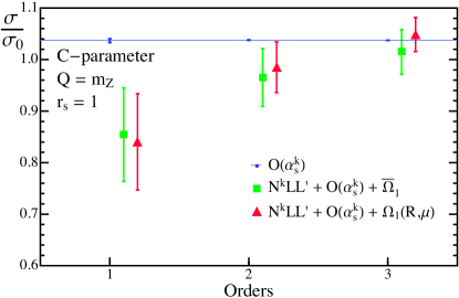
Refer to caption
Refer to caption
Refer to caption
Refer to caption
Figure 10: Total hadronic cross section obtained from integrating the resummed cross section. The top two panels show the prediction for rs=1subscript𝑟𝑠1r_{s}=1 and rs=2subscript𝑟𝑠2r_{s}=2 for C-parameter, respectively. Likewise, the bottom two panels show the thrust results. Green squares correspond to the prediction with log resummation and the power correction in the MS¯¯MS\overline{\textrm{MS}} scheme, whereas red triangles have log resummation and the power correction in the Rgap scheme. The blue points correspond to the fixed-order prediction, and the blue line shows the highest-order FO prediction.
Refer to caption
Figure 11: Components of the C-parameter cross section with resummation at N3LL+𝒪(αs3)+Ω1(R,μ){}^{\prime}+{\cal O}(\alpha_{s}^{3})+\Omega_{1}(R,\mu) with Ω1(RΔ,μΔ)=0.33subscriptΩ1subscript𝑅Δsubscript𝜇Δ0.33\Omega_{1}(R_{\Delta},\mu_{\Delta})=0.33\,GeV and αs(mZ)=0.1141subscript𝛼𝑠subscript𝑚𝑍0.1141\alpha_{s}(m_{Z})=0.1141.

IX.2 The slope 𝐫𝐬subscript𝐫𝐬\mathbf{r_{s}} for C-parameter and Thrust

In the profiles of Sec. VIII, the parameter rssubscript𝑟𝑠r_{s} was defined as the dimensionless slope of μSsubscript𝜇𝑆\mu_{S} in the resummation region. It would seem natural to pick rs=1subscript𝑟𝑠1r_{s}=1 to eliminate the powers of ln(6μS/(QC))6subscript𝜇𝑆𝑄𝐶\ln(6\,\mu_{S}/(QC)) and ln(μS/(Qτ))subscript𝜇𝑆𝑄𝜏\ln(\mu_{S}/(Q\tau)) that appear in the cross section formula for C𝐶C and τ𝜏\tau. However, having a slightly steeper rise may also yield benefits by smoothing out the profile. Using an rssubscript𝑟𝑠r_{s} that is larger than 1, such as rs=2subscript𝑟𝑠2r_{s}=2, will only shift small ln(rs)subscript𝑟𝑠\ln(r_{s}) factors between different orders of the resummed cross section. Just like other profile parameters the dependence on rssubscript𝑟𝑠r_{s} will decrease as we go to higher orders in perturbation theory, but the central value choice may improve the accuracy of lower-order predictions.

In order to determine whether rs=1subscript𝑟𝑠1r_{s}=1 or rs=2subscript𝑟𝑠2r_{s}=2 is a better choice for the slope parameter, we examine the convergence of the cross section between different orders of resummation. For this analysis we will compare the three perturbative orders N3LL+𝒪(αs3){}^{\prime}+{\cal O}(\alpha_{s}^{3}), N2LL+𝒪(αs2){}^{\prime}+{\cal O}(\alpha_{s}^{2}), and NLL+𝒪(αs){}^{\prime}+{\cal O}(\alpha_{s}). We also fix αs(mZ)=0.1141subscript𝛼𝑠subscript𝑚𝑍0.1141\alpha_{s}(m_{Z})=0.1141, which is the value favored by the QCD only thrust fits Abbate et al. (2011). [Use of larger values of αs(mZ)subscript𝛼𝑠subscript𝑚𝑍\alpha_{s}(m_{Z}) leads to the same conclusions that we draw below.] In Fig. 8 we show the perturbative C-parameter cross section (upper two rows) and thrust cross section (lower two rows) with a scan over theory parameters (without including Ω1subscriptΩ1\Omega_{1} or the shape function) for both rs=1subscript𝑟𝑠1r_{s}=1 (first respective row) and rs=2subscript𝑟𝑠2r_{s}=2 (second respective row). Additionally, we plot with different values of Q𝑄Q, using Q=40𝑄40Q=40 GeV in the first column, Q=91.2𝑄91.2Q=91.2 GeV in the second column, and Q=200𝑄200Q=200 GeV in the third column. The bands here correspond to a theory parameter scan with 500500500 random points taken from Tabs. 2 and 3. We conclude from these plots that rs=2subscript𝑟𝑠2r_{s}=2 has better convergence between different orders than rs=1subscript𝑟𝑠1r_{s}=1. For all of the values of Q𝑄Q, we can see that in the slope 1 case the N2LL band lies near the outside of the edge of the NLL band, while in the slope 2 plots, the scan for N2LL is entirely contained within the scan for NLL. A similar picture can be seen for the transition from N2LL to N3LL. This leads us to the conclusion that the resummed cross section prefers rs=2subscript𝑟𝑠2r_{s}=2 profiles which we choose as our central value for the remainder of the analysis. (In the thrust analysis of Ref. Abbate et al. (2011), the profiles did not include an independent slope parameter, but in the resummation region, their profiles are closer to taking rs=2subscript𝑟𝑠2r_{s}=2 than rs=1subscript𝑟𝑠1r_{s}=1.)

Refer to caption
Refer to caption
Refer to caption
Refer to caption
Figure 12: Theory scan for cross section uncertainties in C-parameter. The panels are (a) fixed order, (b) resummation with no nonperturbative function, (c) resummation with a nonperturbative function using the MS¯¯MS\overline{\textrm{MS}} scheme for Ω¯1Csuperscriptsubscript¯Ω1𝐶\overline{\Omega}_{1}^{C} without renormalon subtraction, and (d) resummation with a nonperturbative function using the Rgap scheme for Ω1CsuperscriptsubscriptΩ1𝐶\Omega_{1}^{C} with renormalon subtraction.

At the highest order, N3LL+𝒪(αs3){}^{\prime}+{\cal O}(\alpha_{s}^{3}), the choice of rs=1subscript𝑟𝑠1r_{s}=1 or rs=2subscript𝑟𝑠2r_{s}=2 has very little impact on the resulting cross section, both for C-parameter and thrust. Indeed, the difference between these two choices is smaller than the remaining (small) perturbative uncertainty at this order. This is illustrated in Fig. 9, which shows the complete N3LL+𝒪(αs3)+Ω1(R,μ){}^{\prime}+{\cal O}(\alpha_{s}^{3})+\Omega_{1}(R,\mu) distributions for rs=1subscript𝑟𝑠1r_{s}=1 (blue) and rs=2subscript𝑟𝑠2r_{s}=2 (red) for C-parameter in the left panel, and for thrust in the right panel. Here we use Ω1(RΔ,μΔ)=0.33GeVsubscriptΩ1subscript𝑅Δsubscript𝜇Δ0.33GeV\Omega_{1}(R_{\Delta},\mu_{\Delta})=0.33\,{\rm GeV}. Thus, the choice of rssubscript𝑟𝑠r_{s} is essentially irrelevant for our highest-order predictions, but has a bit of impact on conclusions drawn about the convergence of the lower to highest orders. Another thing that is clear from this figure is that the perturbative uncertainties for the C-parameter cross section at Q=mZ𝑄subscript𝑚𝑍Q=m_{Z}, which are on average ± 2.5%plus-or-minuspercent2.5\pm\,2.5\% in the region 0.25<C<0.650.25𝐶0.650.25<C<0.65, are a bit larger than those for thrust where we have on average ± 1.8%plus-or-minuspercent1.8\pm\,1.8\% in the region 0.1<τ<0.30.1𝜏0.30.1<\tau<0.3. This ± 1.8%plus-or-minuspercent1.8\pm\,1.8\%, obtained with the profile and variations discussed here, agrees well with the ± 1.7%plus-or-minuspercent1.7\pm\,1.7\% quoted in Ref. Abbate et al. (2011).

One can also look at the effect that the choice of rssubscript𝑟𝑠r_{s} has on the total integral over the C-parameter and thrust distributions at NkLL+𝒪(αsk)+Ω1(R,μ){}^{\prime}+{\cal O}(\alpha_{s}^{k})+\Omega_{1}(R,\mu), which should reproduce the total hadronic cross section. For C-parameter, the outcome is shown in the first row of Fig. 10, where green squares and red triangles represent resummed cross sections with power corrections in the MS¯¯MS\overline{\textrm{MS}} and Rgap schemes, respectively. In blue we display the fixed-order prediction. Comparing the predictions for rs=1subscript𝑟𝑠1r_{s}=1 (left panel) and rs=2subscript𝑟𝑠2r_{s}=2 (right panel), we observe that the former achieves a better description of the fixed-order prediction at N2LL, in agreement with observations made in Ref. Alioli et al. (2013). For the case of thrust (second row of Fig. 10), similar conclusions as for C-parameter can be drawn by observing the behavior of the total cross section. Again, at the highest order the result is independent of the choice of the slope within uncertainties for both C𝐶C and thrust. Since our desired fit to determine αs(mZ)subscript𝛼𝑠subscript𝑚𝑍\alpha_{s}(m_{Z}) and Ω1CsuperscriptsubscriptΩ1𝐶\Omega_{1}^{C} requires the best predictions for the shape of the normalized cross section, we do not use the better convergence for the normalization as a criteria for using rs=1subscript𝑟𝑠1r_{s}=1. Our results for cross section shapes are self-normalized using the central profile result.

In Fig. 11 we present a plot analogous to Fig. 5 but including resummation at N3LL+𝒪(αs3)+Ω1(R,μ){}^{\prime}+\,{\cal O}(\alpha_{s}^{3})\,+\,\Omega_{1}(R,\mu) with rs=2subscript𝑟𝑠2r_{s}=2 (a similar plot for thrust can be found in Ref. Abbate et al. (2011)). The suppression of the dashed blue nonsingular curve relative to the solid upper blue singular curve is essentially the same as observed earlier in Fig. 5. The subtraction components are a small part of the cross section in the resummation region but have an impact at the level of precision obtained in our computation. Above the shoulder region, the singular and nonsingular terms appear with opposite signs and largely cancel. This is clear from the figure where the individual singular and nonsingular lines are larger than the total cross section in this region. The same cancellation occurs for the singular subtraction and nonsingular subtraction terms. The black curve labeled total in Fig. 11 shows the central value for our full prediction. Note that the small dip in this black curve, visible at C0.75similar-to-or-equals𝐶0.75C\simeq 0.75, is what survives for the log-singular terms in the shoulder after the convolution with FCsubscript𝐹𝐶F_{C}.

IX.3 Convergence and Uncertainties: Impact of Resummation and Renormalon Subtractions

Results for the C-parameter cross sections at Q=mZ𝑄subscript𝑚𝑍Q=m_{Z} are shown at various levels of theoretical sophistication in Fig. 12. The simplest setup is the purely perturbative fixed-order 𝒪(αsk)𝒪superscriptsubscript𝛼𝑠𝑘{\cal O}(\alpha_{s}^{k}) QCD prediction (i.e. no resummation and no power corrections), shown in panel (a), which does not make use of the new perturbative results in this paper. Not unexpectedly, the most salient feature at fixed order is the lack of overlap between the 𝒪(αs)𝒪subscript𝛼𝑠\mathcal{O}(\alpha_{s}) (green), 𝒪(αs2)𝒪superscriptsubscript𝛼𝑠2\mathcal{O}(\alpha_{s}^{2}) (blue), and 𝒪(αs3)𝒪superscriptsubscript𝛼𝑠3\mathcal{O}(\alpha_{s}^{3}) (red) results. This problem is cured once the perturbative resummation is included with NkLL+𝒪(αsk){}^{\prime}+{\cal O}(\alpha_{s}^{k}) predictions shown in panel (b): the NLL (green), N2LL (blue), and N3LL (red) bands now nicely overlap. To achieve this convergence and overlap with our setup, it is important to normalize the cross section bands with the integrated norm at a given order using the default profiles. (The convergence for the normalization in Fig. 10 was slower. Further discussion of this can be found in Ref. Abbate et al. (2011).)

The panel (b) results neglect power corrections. Including them in the MS¯¯MS\overline{\textrm{MS}} scheme, NkLL+𝒪(αsk)+Ω¯1{}^{\prime}+{\cal O}(\alpha_{s}^{k})+{\overline{\Omega}}_{1}, as shown in panel (c), does not affect the convergence of the series but rather simply shifts the bands toward larger C𝐶C values. This was mentioned above in Eq. (3).
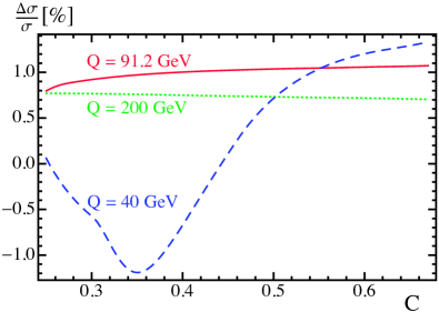
Refer to caption
Refer to caption
Figure 13: Effects of hadron masses on the differential cross section for C-parameter (left) and thrust (right). Curves correspond to the percent difference between the cross section with and without hadron-mass effects, for three center-of-mass energies: Q=91.2𝑄91.2Q=91.2 GeV (solid red), 200200200 GeV (dashed blue), and 404040 GeV (dotted green). The cross section with hadron-mass effects uses θ(RΔ,μΔ)=0𝜃subscript𝑅Δsubscript𝜇Δ0\theta(R_{\Delta},\mu_{\Delta})=0 and Ω1(RΔ,μΔ)=0.32(0.30)subscriptΩ1subscript𝑅Δsubscript𝜇Δ0.320.30\Omega_{1}(R_{\Delta},\mu_{\Delta})=0.32\,(0.30)\,GeV for C-parameter (thrust), while the cross section without hadron-mass effects has Ω1(RΔ,μΔ)=0.33subscriptΩ1subscript𝑅Δsubscript𝜇Δ0.33\Omega_{1}(R_{\Delta},\mu_{\Delta})=0.33\,GeV. We set αs(mZ)=0.1141subscript𝛼𝑠subscript𝑚𝑍0.1141\alpha_{s}(m_{Z})=0.1141.

In panel (d) we show our results, which use the Rgap scheme for the power correction, at NkLL+𝒪(αsk)+Ω1(R,μ){}^{\prime}+{\cal O}(\alpha_{s}^{k})+{\Omega}_{1}(R,\mu). In this scheme a perturbative series is subtracted from the partonic soft function to remove its 𝒪(ΛQCD)𝒪subscriptΛQCD{\cal O}(\Lambda_{\rm QCD}) renormalon. This subtraction entails a corresponding scheme change for the parameter Ω1subscriptΩ1\Omega_{1} which becomes a subtraction-scale-dependent quantity. In general the use of renormalon-free schemes stabilizes the perturbative behavior of cross sections. The main feature visible in panel (d) is the noticeable reduction of the perturbative uncertainty band at the two highest orders, with the bands still essentially contained inside lower-order ones.

We can see the improvement in convergence numerically by comparing the average percent uncertainty between different orders at Q=mZ𝑄subscript𝑚𝑍Q=m_{Z}. If we first look at the results without the renormalon subtraction, at NkLL+𝒪(αsk)+Ω¯1{}^{\prime}+{\cal O}(\alpha_{s}^{k})+{\overline{\Omega}}_{1}, we see that in the region of interest for αs(mZ)subscript𝛼𝑠subscript𝑚𝑍\alpha_{s}(m_{Z}) fits (0.25<C<0.650.25𝐶0.650.25<C<0.65) the NLL distribution has an average percent error of ± 11.7%plus-or-minuspercent11.7\pm\,11.7\%, the N2LL distribution has an average percent error of ± 7.0%plus-or-minuspercent7.0\pm\,7.0\%, and the highest-order N3LL distribution has an average percent error of only ± 4.3%plus-or-minuspercent4.3\pm\,4.3\%. Once we implement the Rgap scheme to remove the renormalon, giving NkLL+𝒪(αsk)+Ω1(R,μ){}^{\prime}+{\cal O}(\alpha_{s}^{k})+{\Omega}_{1}(R,\mu), we see that the NLL distribution has an average percent error of ± 11.8%plus-or-minuspercent11.8\pm\,11.8\%, the N2LL distribution has an average percent error of ± 4.9%plus-or-minuspercent4.9\pm\,4.9\%, and the most precise N3LL distribution has an average percent error of only ± 2.5%plus-or-minuspercent2.5\pm\,2.5\%. Although the renormalon subtractions for C-parameter induce a trend toward the lower edge of the perturbative band of the predictions at one lower order, the improved convergence of the perturbative series makes the use of these more accurate predictions desirable.
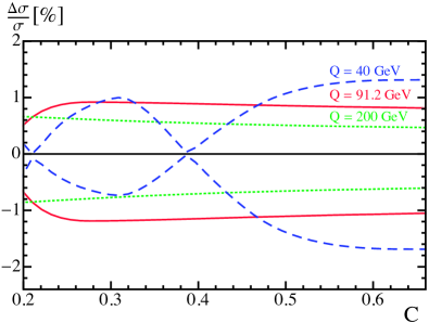
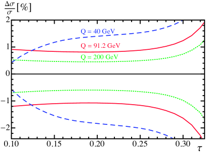
Refer to caption
Refer to caption
Figure 14: Effects of θ(RΔ,μΔ)𝜃subscript𝑅Δsubscript𝜇Δ\theta(R_{\Delta},\mu_{\Delta}) on the cross section for C-parameter (left) and thrust (right). The lines correspond to the largest variation achievable by varying θ(RΔ,μΔ)𝜃subscript𝑅Δsubscript𝜇Δ\theta(R_{\Delta},\mu_{\Delta}) in both directions (which happen for θ=0.23π𝜃0.23𝜋\theta=0.23\,\pi and θ= 0.27π𝜃0.27𝜋\theta=-\,0.27\,\pi), with respect to the cross section with θ(RΔ,μΔ)=0𝜃subscript𝑅Δsubscript𝜇Δ0\theta(R_{\Delta},\mu_{\Delta})=0. The solid (red), dashed (blue), and dotted (green) lines correspond to Q=91.2𝑄91.2Q=91.2, 200200200, and 404040 GeV, respectively. We use Ω1(RΔ,μΔ)=0.32(0.30)subscriptΩ1subscript𝑅Δsubscript𝜇Δ0.320.30\Omega_{1}(R_{\Delta},\mu_{\Delta})=0.32\,(0.30)\,GeV for C-parameter (thrust), and αs(mZ)=0.1141subscript𝛼𝑠subscript𝑚𝑍0.1141\alpha_{s}(m_{Z})=0.1141.

IX.4 Impact of Hadron Mass Effects

In this section we discuss the impact of adding hadron-mass effects, which gives the orders denoted NkLL+𝒪(αsk)+Ω1(R,μ,r){}^{\prime}+{\cal O}(\alpha_{s}^{k})+{\Omega}_{1}(R,\mu,r). Hadron masses induce an additional anomalous dimension for Ω1subscriptΩ1\Omega_{1} and an associated series of logarithms of the form ln(QC/ΛQCD)𝑄𝐶subscriptΛQCD\ln(QC/\Lambda_{\rm QCD}) that need to be resummed. They also impact the definition of Ω1subscriptΩ1\Omega_{1} and its RGE equations in the MS¯¯MS\overline{\rm MS} and Rgap schemes. Since the overall effect of hadron masses on C-parameter and thrust are rather small, they do not change the perturbative convergence discussed in the previous section. Therefore, we study these effects here making use of only the highest-order perturbative results at N3LL+𝒪(αs3){}^{\prime}+{\cal O}(\alpha_{s}^{3}).

In Fig. 13 we show the effect of hadron-mass running on the cross section. We compare differential cross sections with and without hadron masses, at the same center-of-mass energies. When the running effects from hadron masses are turned off, the value of Ω1(RΔ,μΔ)subscriptΩ1subscript𝑅Δsubscript𝜇Δ\Omega_{1}(R_{\Delta},\mu_{\Delta}) preferred by the experimental data will attempt to average away these effects by absorbing them into the value of the initial parameter. (The running of Ω1subscriptΩ1\Omega_{1} with and without hadron masses is shown below in Fig. 19.) Therefore, the specific values used in Fig. 13 are obtained by fixing αs(mZ)subscript𝛼𝑠subscript𝑚𝑍\alpha_{s}(m_{Z}) and then fitting for Ω1(RΔ,μΔ)subscriptΩ1subscript𝑅Δsubscript𝜇Δ\Omega_{1}(R_{\Delta},\mu_{\Delta}) to minimize the difference between the cross section with and without hadron masses in the tail region. As the values for αs(mZ)subscript𝛼𝑠subscript𝑚𝑍\alpha_{s}(m_{Z}) and Ω1subscriptΩ1\Omega_{1} in the case of no hadron-mass effects come from a fit to data (from Ref. Abbate et al. (2011)), choosing Ω1(RΔ,μΔ)subscriptΩ1subscript𝑅Δsubscript𝜇Δ\Omega_{1}(R_{\Delta},\mu_{\Delta}) with the outlined procedure is similar to a full fit to data and will give results that allow comparison between the two cases. With hadron masses on, we fix θ(RΔ,μΔ)=0𝜃subscript𝑅Δsubscript𝜇Δ0\theta(R_{\Delta},\mu_{\Delta})=0, so the effects observed in Fig. 13 are related to the additional log resummation for Ω1subscriptΩ1\Omega_{1}. The effect is largest at Q=40𝑄40Q=40\,GeV where it varies between a  1.25%percent1.25-\,1.25\% and + 1.25%percent1.25+\,1.25\% shift for C-parameter and between a  1.5%percent1.5-\,1.5\% and + 0.5%percent0.5+\,0.5\% shift for thrust. For Q=mZ𝑄subscript𝑚𝑍Q=m_{Z} it amounts to a 1.0%percent1.01.0\% shift for C-parameter and a shift of 0%percent00\% to 1.3%percent1.31.3\% for thrust.

With hadron masses the additional hadronic parameter θ(RΔ,μΔ)𝜃subscript𝑅Δsubscript𝜇Δ\theta(R_{\Delta},\mu_{\Delta}) encodes the fact that the extra resummation takes place in r𝑟r space, and therefore induces some dependence on the shape of the Ω1(R,μ,r)subscriptΩ1𝑅𝜇𝑟\Omega_{1}(R,\mu,r) parameter. In contrast the dominant hadronic parameter Ω1(RΔ,μΔ)subscriptΩ1subscript𝑅Δsubscript𝜇Δ\Omega_{1}(R_{\Delta},\mu_{\Delta}) is the normalization of this r𝑟r-space hadronic function. In Fig. 14 we show the effect that varying π/2<θ(RΔ,μΔ)<π/2𝜋2𝜃subscript𝑅Δsubscript𝜇Δ𝜋2-\,\pi/2<\theta(R_{\Delta},\mu_{\Delta})<\pi/2 has on the cross section for three center-of-mass energies, fixing Ω1(RΔ,μΔ)=320subscriptΩ1subscript𝑅Δsubscript𝜇Δ320\Omega_{1}(R_{\Delta},\mu_{\Delta})=320 MeV for C-parameter and 300300300 MeV for thrust. The sensitivity of ΔσΔ𝜎\Delta\sigma here is proportional to Ω1(RΔ,μΔ)subscriptΩ1subscript𝑅Δsubscript𝜇Δ\Omega_{1}(R_{\Delta},\mu_{\Delta}). In these plots we pick the value of θ𝜃\theta that gives the largest deviation from the θ=0𝜃0\theta=0 cross section (these values are listed in the figure caption). This maximum deviation is only 1.5%percent1.51.5\% for C-parameter and occurs at Q=40𝑄40Q=40 GeV at larger C𝐶C. For thrust, the largest deviation also occurs for Q=40𝑄40Q=40 GeV and for higher values of τ𝜏\tau and is 2.0%less-than-or-similar-toabsentpercent2.0\lesssim 2.0\% for τ0.3𝜏0.3\tau\leq 0.3. For Q=mZ𝑄subscript𝑚𝑍Q=m_{Z} the effect is roughly ±1.0%plus-or-minuspercent1.0\pm 1.0\% for C-parameter and around 1.0%percent1.01.0\% for thrust when τ<0.25𝜏0.25\tau<0.25, growing to 2%percent22\% by τ=0.33𝜏0.33\tau=0.33.

We conclude that the effect of hadron masses on log resummation should be included if one wishes to avoid an additional 1.5%similar-toabsentpercent1.5\sim 1.5\% uncertainty on the cross section. Furthermore, one should consider fitting θ(RΔ,μΔ)𝜃subscript𝑅Δsubscript𝜇Δ\theta(R_{\Delta},\mu_{\Delta}) as an additional parameter if one wants to avoid another 1%similar-toabsentpercent1\sim 1\% uncertainty in the cross section that it induces. (Recall that Fig. 14 shows the worst-case scenario.)

X Conclusions

We have provided a factorization formula for the C-parameter distribution in e+esuperscript𝑒superscript𝑒e^{+}e^{-} annihilation and analyzed its utility in making precision cross section predictions, extending earlier work on thrust Abbate et al. (2011). We have determined or computed the ingredients needed to achieve a summation of large logarithms at N3LL order for the singular terms in the dijet limit where C𝐶C is small, pushing beyond the classical resummed computations in Ref. Catani and Webber (1998) by two additional orders. To achieve this goal, we demonstrated that the anomalous dimensions, as well as the hard and jet functions, are identical in the C-parameter and thrust distributions to all orders in perturbation theory. We then computed the only distinct piece, the soft function, to one-loop order analytically, two-loop order numerically, and with logarithmic accuracy at three loops using its anomalous dimension. (We also present a master formula for the one-loop soft function, valid for any recoil-free dijet event shape, in App. C.) Our factorization formula also incorporates the previously known 𝒪(αs2)𝒪superscriptsubscript𝛼𝑠2{\cal O}(\alpha_{s}^{2}) and 𝒪(αs3)𝒪superscriptsubscript𝛼𝑠3{\cal O}(\alpha_{s}^{3}) perturbative QCD corrections in fixed order Gehrmann-De Ridder et al. (2007a, b, 2009); Gehrmann-De Ridder et al. (2014); Weinzierl (2008, 2009).

Using our factorization theorem and computation for the soft function, we were able to analytically predict the fixed-order log-singular terms of C-parameter up to 𝒪(αs3)𝒪superscriptsubscript𝛼𝑠3{\cal O}(\alpha_{s}^{3}). These results were used to consistently incorporate fixed-order results at the same order by subtracting them from the numerical 𝒪(αs3)𝒪superscriptsubscript𝛼𝑠3{\cal O}(\alpha_{s}^{3}) results, to obtain the nonsingular terms plotted in Figs. 2, 3, and 4 and compared to the singular cross section in Fig. 5.

The factorization formula we used incorporates a systematic description of nonperturbative power corrections using a shape function FCsubscript𝐹𝐶F_{C}, whose moments are given by quantum field theory matrix elements. This nonperturative shape function describes the dynamics of soft particle radiation at large angles. Although the shape function of thrust and C-parameter are a priori unrelated, one can show that, up to small deviations caused by hadron masses, their respective first moments are proportional to each other involving a simple calculable coefficient, as shown in Eq. (2). Tests of this universality are very important, since the first moment of the shape function constitutes the most important nonperturative power correction in the tail of the distribution, where one can write down an OPE for the event-shape distributions. The results in this paper allow for universality to be tested with data accounting for a high degree of perturbative precision and incorporating hadron-mass effects.

In order to reduce the sensitivity to an 𝒪(ΛQCD)𝒪subscriptΛQCD\mathcal{O}(\Lambda_{\rm QCD}) renormalon present in the soft function, we switched to a short-distance scheme for the leading power correction, which translates into a more stable perturbative behavior. Using universality relations, it is possible (and desirable) to use thrust gap subtractions in the C-parameter distribution, with the appropriate prefactor. Furthermore, we introduced hadron-mass running effects into this formalism, and showed how one can consistently account for Rgap and hadron-mass running simultaneously.

We have used profile functions, which are C𝐶C-dependent renormalization scales, to both properly implement the required conditions for the scales in different regions in Eq. (VIII), including the resummation of large logarithms in the nonperturbative and resummation regions, and to smoothly carry out the transition between regions. There are two significant differences for the C-parameter relative to thrust: the nonperturbative region is enlarged by a factor 3π/23𝜋23\pi/2, and the slope of μSsubscript𝜇𝑆\mu_{S} in the resummation region is reduced by a factor of 666. In Sec. IX.2 we made a numerical investigation of possible choices for the slope of the soft function in the resummation region and concluded both for thrust and C-parameter that having a slope that is twice the canonical value, rs=2subscript𝑟𝑠2r_{s}=2 rather than rs=1subscript𝑟𝑠1r_{s}=1, is advantageous to have a better order-by-order convergence. At the highest order we achieves, which is N3LL, we also observe that the choice of rs=1subscript𝑟𝑠1r_{s}=1 versus rs=2subscript𝑟𝑠2r_{s}=2 becomes irrelevant.

Our most accurate theoretical description has a very good perturbative convergence, and achieves a perturbative uncertainty of on average 2.5%percent2.52.5\% in the tail of the distribution for Q=mZ𝑄subscript𝑚𝑍Q=m_{Z}; see Fig. 12. We have also shown that the effect of hadron-mass corrections is at the <2%absentpercent2<2\% level (depending on Q𝑄Q, and differing somewhat between C-parameter and thrust); see Figs. 13 and 14. The theory developments made here are necessary for a high-precision determination of the strong coupling constant αs(mZ)subscript𝛼𝑠subscript𝑚𝑍\alpha_{s}(m_{Z}) by fits to experimental data. Moreover, by simultaneously fitting to the leading power correction Ω1subscriptΩ1\Omega_{1}, our formalism allows us to check for universality between thrust and C-parameter, exploiting the high level of perturbative precision and also accounting for hadron-mass effects. These results will be presented in a separate paper Hoang et al. (2015a).

Acknowledgements.
This work was supported by the offices of Nuclear Physics of the U.S. Department of Energy (DOE) under under Contract No. DE-SC0011090 and the European Community’s Marie-Curie Research Networks under contract PITN-GA-2010-264564 (LHCphenOnet). IS was also supported in part by the Simons Foundation Investigator Grant No. 327942. VM was supported by a Marie Curie Fellowship under Contract No. PIOF-GA-2009-251174 while part of this work was completed. This work was also supported in part by MIT MISTI global seed funds and the ESI summer program on “Jets and Quantum Fields for the LHC and Future Colliders”. VM thanks Thomas Hahn for computing support. We thank Thomas Gehrmann for providing us with numerical results from the program EERAD3.

Appendix A Formulae

In this appendix we collect all the remaining formulae used in our analysis for the case of massless quarks. Since we want to compare to experimental data, which are normalized to the total number of events, we need to calculate (1/σ)dσ/dC1𝜎d𝜎d𝐶(1/\sigma)\mathrm{d}\sigma/\mathrm{d}C, our normalized cross section. To do this we can either self-normalize our results by integrating over C𝐶C or use the fixed-order result for the total hadronic cross section, which, at three loops for massless quarks at μ=Q𝜇𝑄\mu=Q, is (see Ref. Chetyrkin et al. (1996) for further discussion)

Rhadsubscript𝑅had\displaystyle R_{\rm had}\, = 1+0.3183099αs(Q)+0.1427849αs2(Q)absent10.3183099subscript𝛼𝑠𝑄0.1427849superscriptsubscript𝛼𝑠2𝑄\displaystyle=\,1+0.3183099\,\alpha_{s}(Q)+0.1427849\,\alpha_{s}^{2}(Q)
 0.411757αs3(Q).0.411757superscriptsubscript𝛼𝑠3𝑄\displaystyle\ -\,0.411757\,\alpha_{s}^{3}(Q)\,. (82)

Throughout our analysis, we use mZ=91.187GeVsubscript𝑚𝑍91.187GeVm_{Z}=91.187\,\mathrm{GeV}, and all numerical results quoted below are for SU(3) color with nf=5subscript𝑛𝑓5n_{f}=5 active light flavors, for simplicity.

Singular Cross Section Formula

For the singular part of the differential cross section given in Eq. (29), we simplify the numerical evaluation using our freedom to take μ=μJ𝜇subscript𝜇𝐽\mu=\mu_{J}. This means UJτ(ss,μJ,μJ)=δ(ss)superscriptsubscript𝑈𝐽𝜏𝑠superscript𝑠subscript𝜇𝐽subscript𝜇𝐽𝛿𝑠superscript𝑠U_{J}^{\tau}(s-s^{\prime},\mu_{J},\mu_{J})=\delta(s-s^{\prime}), and we can write

1σ0dkdσ^sdC(CkQ)FC(k3πΔ¯(R,μS))1subscript𝜎0differential-d𝑘dsubscript^𝜎𝑠d𝐶𝐶𝑘𝑄subscript𝐹𝐶𝑘3𝜋¯Δ𝑅subscript𝜇𝑆\displaystyle\frac{1}{\sigma_{0}}\!\int\!{\rm d}k\,\frac{{\rm d}\hat{\sigma}_{s}}{{\rm d}C}\Big{(}C-\frac{k}{Q}\Big{)}F_{C}\Big{(}k-3\pi\bar{\Delta}(R,\mu_{S})\Big{)}
=Q6H(Q,μH)UH(Q,μH,μJ)absent𝑄6𝐻𝑄subscript𝜇𝐻subscript𝑈𝐻𝑄subscript𝜇𝐻subscript𝜇𝐽\displaystyle=\frac{Q}{6}H(Q,{\mu}_{H})\,U_{H}\big{(}Q,{\mu}_{H},{\mu}_{J}\big{)}\,
×dkP(Q,QC/6k/6,μJ)\displaystyle\times\int{\rm d}k\,P\big{(}Q,QC/6-k/6,{\mu}_{J}\big{)}\,
×e3πδ(R,μs)ddkFC(k3πΔ¯(R,μS)),absentsuperscript𝑒3𝜋𝛿𝑅subscript𝜇𝑠dd𝑘subscript𝐹𝐶𝑘3𝜋¯Δ𝑅subscript𝜇𝑆\displaystyle\times e^{-{3\pi\,\delta(R,\mu_{s})}\frac{{\rm d}}{{\rm d}k}}\,F_{C}\Big{(}k-3\pi\,\bar{\Delta}(R,\mu_{S})\Big{)}, (83)

Here σ0subscript𝜎0\sigma_{0} is the tree-level (Born) cross section for e+eqq¯superscript𝑒superscript𝑒𝑞¯𝑞e^{+}e^{-}\to q\bar{q}. Here we have combined the perturbative corrections from the partonic soft function, jet function, and soft evolution factor into a single function,

P(Q,k,μJ)𝑃𝑄𝑘subscript𝜇𝐽\displaystyle P(Q,k,\mu_{J}) =dsdkJτ(s,μJ)USτ(k,μJ,μS)absentdifferential-d𝑠differential-dsuperscript𝑘subscript𝐽𝜏𝑠subscript𝜇𝐽superscriptsubscript𝑈𝑆𝜏superscript𝑘subscript𝜇𝐽subscript𝜇𝑆\displaystyle=\int\!{\rm d}s\!\int\!{\rm d}k^{\prime}J_{\tau}(s,\mu_{J})\,U_{S}^{\tau}(k^{\prime},\mu_{J},\mu_{S})
×S^C~(kks/Q,μS).absentsubscript^𝑆~𝐶𝑘superscript𝑘𝑠𝑄subscript𝜇𝑆\displaystyle\times\hat{S}_{\widetilde{C}}(k-k^{\prime}-s/Q,\mu_{S})\ \,. (84)

The large logarithms of C/6𝐶6C/6 are summed up in the evolution factors UHsubscript𝑈𝐻U_{H} and USτsuperscriptsubscript𝑈𝑆𝜏U_{S}^{\tau}. We can carry out the integrals in P𝑃P exactly, and the results are enumerated below. The shape function FC(k3πΔ¯)subscript𝐹𝐶𝑘3𝜋¯ΔF_{C}(k-3\pi\,\bar{\Delta}) is discussed in Sec. VII, and we have used integration by parts in Eq. (A) to have the derivative in the exponential act on FCsubscript𝐹𝐶F_{C}, which is simpler than acting the derivative on the perturbative soft function. For our numerical calculation, we expand H𝐻H, Jτsubscript𝐽𝜏J_{\tau}, and S^C~subscript^𝑆~𝐶\hat{S}_{\widetilde{C}} order by order as a series in αs(μH)subscript𝛼𝑠subscript𝜇𝐻\alpha_{s}(\mu_{H}), αs(μJ)subscript𝛼𝑠subscript𝜇𝐽\alpha_{s}(\mu_{J}), and αs(μS)subscript𝛼𝑠subscript𝜇𝑆\alpha_{s}(\mu_{S}) respectively, with no large logs. Additionally, we expand exp( 3πδ(R,μS)d/dk)3𝜋𝛿𝑅subscript𝜇𝑆dd𝑘\exp(-\,3\pi\,\delta(R,\mu_{S}){\rm d}/{\rm d}k) [see Eq. (49)] as a series in αs(μS)subscript𝛼𝑠subscript𝜇𝑆\alpha_{s}(\mu_{S}), which must be done consistently to cancel the renormalon present in S^C~subscript^𝑆~𝐶\hat{S}_{\widetilde{C}}.

The hard function to 𝒪(αs3)𝒪superscriptsubscript𝛼𝑠3{\cal O}(\alpha_{s}^{3}) with nf=5subscript𝑛𝑓5n_{f}=5 is Matsuura and van Neerven (1988); Matsuura et al. (1989); Gehrmann et al. (2005); Moch et al. (2005); Lee et al. (2010); Baikov et al. (2009); Gehrmann et al. (2010); Abbate et al. (2011)

H(Q,μH)𝐻𝑄subscript𝜇𝐻\displaystyle H(Q,\mu_{H})
=1+αs(μH)(0.7458081.27324LQ0.848826LQ2)absent1subscript𝛼𝑠subscript𝜇𝐻0.7458081.27324subscript𝐿𝑄0.848826superscriptsubscript𝐿𝑄2\displaystyle=1+\alpha_{s}(\mu_{H})\Big{(}\!0.745808\!-\!1.27324L_{Q}\!-\!0.848826L_{Q}^{2}\Big{)}
+αs2(μH)(2.275870.0251035LQ1.06592LQ2\displaystyle+\alpha_{s}^{2}(\mu_{H})\Big{(}2.27587-0.0251035\,L_{Q}-1.06592\,L_{Q}^{2}
+0.735517LQ3+0.360253LQ4)\displaystyle+0.735517L_{Q}^{3}+0.360253L_{Q}^{4}\Big{)}
+αs3(μH)(0.00050393h3+2.78092LQ2.85654LQ2\displaystyle+\alpha_{s}^{3}(\mu_{H})\Big{(}0.00050393\,h_{3}+2.78092L_{Q}-2.85654L_{Q}^{2}
0.147051LQ3+0.865045LQ40.165638LQ50.147051superscriptsubscript𝐿𝑄30.865045superscriptsubscript𝐿𝑄40.165638superscriptsubscript𝐿𝑄5\displaystyle-0.147051L_{Q}^{3}+0.865045L_{Q}^{4}-0.165638L_{Q}^{5}
0.101931LQ6),\displaystyle-0.101931\,L_{Q}^{6}\Big{)}\,, (85)

where LQ=lnμHQsubscript𝐿𝑄subscript𝜇𝐻𝑄L_{Q}=\ln\frac{{\mu}_{H}}{Q} and h3=8998.080subscript38998.080h_{3}=8998.080 from Ref. Baikov et al. (2009).

The resummation of large logs between μHsubscript𝜇𝐻\mu_{H} and μJsubscript𝜇𝐽\mu_{J} is given by UH(Q,μH,μJ)subscript𝑈𝐻𝑄subscript𝜇𝐻subscript𝜇𝐽U_{H}(Q,{\mu}_{H},{\mu}_{J}), the solution of the RGE for the hard function, which can be written as Bauer et al. (2001b)

UH(Q,μH,μ)=e2K(ΓH,γH,μ,μH)(μH2Q2)ω(ΓH,μ,μH),subscript𝑈𝐻𝑄subscript𝜇𝐻𝜇superscript𝑒2𝐾subscriptΓ𝐻subscript𝛾𝐻𝜇subscript𝜇𝐻superscriptsuperscriptsubscript𝜇𝐻2superscript𝑄2𝜔subscriptΓ𝐻𝜇subscript𝜇𝐻\displaystyle U_{H}(Q,{\mu}_{H},{\mu})=e^{2K(\Gamma_{H},\gamma_{H},{\mu},{\mu}_{H})}\bigg{(}\frac{{\mu}_{H}^{2}}{Q^{2}}\bigg{)}^{\!\!\omega(\Gamma_{H}\!,\,{\mu},{\mu}_{H})}, (86)

where ω𝜔\omega and K𝐾K are given in Eqs. (A) and (A) below.

In momentum space, we can use the results from Ref. Ligeti et al. (2008) to calculate the convolution of the plus-functions in P𝑃P to give the form

P(Q,k,μJ)=1ξES(ξ,μJ,μS)𝑃𝑄𝑘subscript𝜇𝐽1𝜉subscript𝐸𝑆𝜉subscript𝜇𝐽subscript𝜇𝑆\displaystyle P\big{(}Q,k,{\mu}_{J}\big{)}=\frac{1}{\xi}\,E_{S}\big{(}\xi,{\mu}_{J},{\mu}_{S}\big{)}
×n,m,k,l=1m+n+1kk+1lVkmnJm[αs(μJ),ξQμJ2]SnC~[αs(μS),ξμS]\displaystyle\times\sum_{\begin{subarray}{c}n,m,k,l=-1\\ m+n+1\geq k\\ k+1\geq l\end{subarray}}^{\infty}V_{k}^{mn}\,\,J_{m}\Big{[}\alpha_{s}({\mu}_{J}),\frac{\xi\,Q}{{\mu}^{2}_{J}}\Big{]}\,S_{n}^{\widetilde{C}}\Big{[}\alpha_{s}({\mu}_{S}),\frac{\xi}{{\mu}_{S}}\Big{]}\,
×Vlk[2ω(ΓS,μJ,μS)]l2ω(ΓS,μJ,μS)(kξ).absentsuperscriptsubscript𝑉𝑙𝑘delimited-[]2𝜔subscriptΓ𝑆subscript𝜇𝐽subscript𝜇𝑆superscriptsubscript𝑙2𝜔subscriptΓ𝑆subscript𝜇𝐽subscript𝜇𝑆𝑘𝜉\displaystyle\times V_{l}^{k}\big{[}-2\,\omega(\Gamma_{S},{\mu}_{J},{\mu}_{S})\big{]}\,\mathcal{L}_{l}^{-2\omega(\Gamma_{S},{\mu}_{J},{\mu}_{S})}\Big{(}\frac{k}{\xi}\Big{)}\,. (87)

Here ξ𝜉\xi is a dummy variable that does not affect the value of the result. 666When convolved with FCsubscript𝐹𝐶F_{C} we use our freedom in choosing ξ𝜉\xi to simplify the final numerical integration, picking ξ=QC/63πΔ¯(R,μS)𝜉𝑄𝐶63𝜋¯Δ𝑅subscript𝜇𝑆\xi=QC/6-3\pi\,\bar{\Delta}(R,\mu_{S}). ES(ξ,μJ,μS)subscript𝐸𝑆𝜉subscript𝜇𝐽subscript𝜇𝑆E_{S}(\xi,\mu_{J},\mu_{S}) is given by Balzereit et al. (1998); Neubert (2005)

ES(ξ,μJ,μS)=exp[2K(ΓS,γS,μJ,μS)]subscript𝐸𝑆𝜉subscript𝜇𝐽subscript𝜇𝑆2𝐾subscriptΓ𝑆subscript𝛾𝑆subscript𝜇𝐽subscript𝜇𝑆\displaystyle E_{S}(\xi,{\mu}_{J},{\mu}_{S})=\exp\!\big{[}2K(\Gamma_{S},\gamma_{S},{\mu}_{J},{\mu}_{S})\big{]} (88)
×(ξμS)2ω(ΓS,μJ,μS)exp[2γEω(ΓS,μJ,μS)]Γ[12ω(ΓS,μJ,μS)],absentsuperscript𝜉subscript𝜇𝑆2𝜔subscriptΓ𝑆subscript𝜇𝐽subscript𝜇𝑆2subscript𝛾𝐸𝜔subscriptΓ𝑆subscript𝜇𝐽subscript𝜇𝑆Γdelimited-[]12𝜔subscriptΓ𝑆subscript𝜇𝐽subscript𝜇𝑆\displaystyle\times\Big{(}\frac{\xi}{{\mu}_{S}}\Big{)}^{-2\omega(\Gamma_{S},{\mu}_{J},{\mu}_{S})}\ \frac{\exp\!\big{[}2\gamma_{E}\,\omega(\Gamma_{S},{\mu}_{J},{\mu}_{S})\big{]}}{\Gamma\big{[}1-2\,\omega(\Gamma_{S},{\mu}_{J},{\mu}_{S})\big{]}}\,,

and encodes part of the running between μSsubscript𝜇𝑆\mu_{S} and μJsubscript𝜇𝐽\mu_{J}. The rest of the running is included in the V𝑉V coefficients and the plus-functions, lsubscript𝑙\mathcal{L}_{l}.

The Jmsubscript𝐽𝑚J_{m} and Snsubscript𝑆𝑛S_{n} in Eq. (A) are the coefficients of the momentum-space soft and jet functions, given by

Jτ(pk,μJ)subscript𝐽𝜏superscript𝑝𝑘subscript𝜇𝐽\displaystyle J_{\tau}(p^{-}k,\mu_{J}) =1pξm=1Jm[αs(μJ),pξμJ2]m(kξ),absent1superscript𝑝𝜉superscriptsubscript𝑚1subscript𝐽𝑚subscript𝛼𝑠subscript𝜇𝐽superscript𝑝𝜉superscriptsubscript𝜇𝐽2subscript𝑚𝑘𝜉\displaystyle=\frac{1}{p^{-}\xi}\sum_{m=-1}^{\infty}J_{m}\Big{[}\alpha_{s}(\mu_{J}),\frac{p^{-}\xi}{\mu_{J}^{2}}\Big{]}{\cal L}_{m}\Big{(}\frac{k}{\xi}\Big{)},
S^C~(k,μS)subscript^𝑆~𝐶𝑘subscript𝜇𝑆\displaystyle\hat{S}_{\widetilde{C}}(k,\mu_{S}) =1ξn=1SnC~[αs(μS),ξμS]n(kξ).absent1𝜉superscriptsubscript𝑛1superscriptsubscript𝑆𝑛~𝐶subscript𝛼𝑠subscript𝜇𝑆𝜉subscript𝜇𝑆subscript𝑛𝑘𝜉\displaystyle=\frac{1}{\xi}\sum_{n=-1}^{\infty}S_{n}^{\widetilde{C}}\Big{[}\alpha_{s}(\mu_{S}),\frac{\xi}{\mu_{S}}\Big{]}{\cal L}_{n}\Big{(}\frac{k}{\xi}\Big{)}. (89)

Here the C-parameter soft function coefficients are

S1C~[αs,x]superscriptsubscript𝑆1~𝐶subscript𝛼𝑠𝑥\displaystyle S_{-1}^{\widetilde{C}}[\alpha_{s},x] =S1C~(αs)+n=0SnC~(αs)lnn+1xn+1,absentsuperscriptsubscript𝑆1~𝐶subscript𝛼𝑠superscriptsubscript𝑛0superscriptsubscript𝑆𝑛~𝐶subscript𝛼𝑠superscript𝑛1𝑥𝑛1\displaystyle=S_{-1}^{\widetilde{C}}(\alpha_{s})+\sum_{n=0}^{\infty}S_{n}^{\widetilde{C}}(\alpha_{s})\frac{\ln^{n+1}x}{n+1}\,,
SnC~[αs,x]superscriptsubscript𝑆𝑛~𝐶subscript𝛼𝑠𝑥\displaystyle S_{n}^{\widetilde{C}}[\alpha_{s},x] =k=0(n+k)!n!k!Sn+kC~(αs)lnkx,absentsuperscriptsubscript𝑘0𝑛𝑘𝑛𝑘superscriptsubscript𝑆𝑛𝑘~𝐶subscript𝛼𝑠superscript𝑘𝑥\displaystyle=\sum_{k=0}^{\infty}\frac{(n+k)!}{n!\,k!}S_{n+k}^{\widetilde{C}}(\alpha_{s})\ln^{k}x\,, (90)

which for nf=5subscript𝑛𝑓5n_{f}=5 can be written as

S1C~(αs)superscriptsubscript𝑆1~𝐶subscript𝛼𝑠\displaystyle S_{-1}^{\widetilde{C}}(\alpha_{s}) =1+1.0472αs+(1.75598+0.012666s2C~)αs2absent11.0472subscript𝛼𝑠1.755980.012666superscriptsubscript𝑠2~𝐶superscriptsubscript𝛼𝑠2\displaystyle=1+1.0472\alpha_{s}+(1.75598+0.012666\,s_{2}^{\widetilde{C}})\alpha_{s}^{2}
+(2.59883+0.0132629s2C~+0.00100786s3C~)αs3,2.598830.0132629superscriptsubscript𝑠2~𝐶0.00100786superscriptsubscript𝑠3~𝐶superscriptsubscript𝛼𝑠3\displaystyle+\left(2.59883+0.0132629\,s_{2}^{\widetilde{C}}+0.00100786\,s_{3}^{\widetilde{C}}\right)\alpha_{s}^{3}\,,
S0C~(αs)superscriptsubscript𝑆0~𝐶subscript𝛼𝑠\displaystyle S_{0}^{\widetilde{C}}(\alpha_{s}) =1.22136αs2+(2.634810.0309077s2C~)αs3,absent1.22136superscriptsubscript𝛼𝑠22.634810.0309077superscriptsubscript𝑠2~𝐶superscriptsubscript𝛼𝑠3\displaystyle=1.22136\alpha_{s}^{2}+(2.63481-0.0309077\,s_{2}^{\widetilde{C}})\alpha_{s}^{3}\,,
S1C~(αs)superscriptsubscript𝑆1~𝐶subscript𝛼𝑠\displaystyle S_{1}^{\widetilde{C}}(\alpha_{s}) =1.69765αs7.45178αs2absent1.69765subscript𝛼𝑠7.45178superscriptsubscript𝛼𝑠2\displaystyle=-1.69765\,\alpha_{s}-7.45178\,\alpha_{s}^{2}
(19.1773+0.021501s2C~)αs3,19.17730.021501superscriptsubscript𝑠2~𝐶superscriptsubscript𝛼𝑠3\displaystyle-(19.1773+0.021501\,s_{2}^{\widetilde{C}})\,\alpha_{s}^{3}\,,
S2C~(αs)superscriptsubscript𝑆2~𝐶subscript𝛼𝑠\displaystyle S_{2}^{\widetilde{C}}(\alpha_{s}) =1.03573αs2+2.3245αs3,absent1.03573superscriptsubscript𝛼𝑠22.3245superscriptsubscript𝛼𝑠3\displaystyle=1.03573\,\alpha_{s}^{2}+2.3245\,\alpha_{s}^{3}\,,
S3C~(αs)superscriptsubscript𝑆3~𝐶subscript𝛼𝑠\displaystyle S_{3}^{\widetilde{C}}(\alpha_{s}) =1.44101αs2+10.299αs3,absent1.44101superscriptsubscript𝛼𝑠210.299superscriptsubscript𝛼𝑠3\displaystyle=1.44101\,\alpha_{s}^{2}+10.299\,\alpha_{s}^{3}\,,
S4C~(αs)superscriptsubscript𝑆4~𝐶subscript𝛼𝑠\displaystyle S_{4}^{\widetilde{C}}(\alpha_{s}) = 1.46525αs3,absent1.46525superscriptsubscript𝛼𝑠3\displaystyle=-\,1.46525\,\alpha_{s}^{3}\,,
S5C~(αs)superscriptsubscript𝑆5~𝐶subscript𝛼𝑠\displaystyle S_{5}^{\widetilde{C}}(\alpha_{s}) = 0.611585αs3.absent0.611585superscriptsubscript𝛼𝑠3\displaystyle=-\,0.611585\,\alpha_{s}^{3}\,. (91)

Note that s2C~superscriptsubscript𝑠2~𝐶s_{2}^{\widetilde{C}} and s3C~superscriptsubscript𝑠3~𝐶s_{3}^{\widetilde{C}} are the 𝒪(αs2,3)𝒪superscriptsubscript𝛼𝑠23{\cal O}(\alpha_{s}^{2,3}) coefficients of the non-logarithmic terms in the series expansion of the logarithm of the position space C-parameter soft function. The coefficients for the jet function are

J1[αs,x]=subscript𝐽1subscript𝛼𝑠𝑥absent\displaystyle J_{-1}[\alpha_{s},x]= J1(αs)+n=0Jn(αs)lnn+1xn+1,subscript𝐽1subscript𝛼𝑠superscriptsubscript𝑛0subscript𝐽𝑛subscript𝛼𝑠superscript𝑛1𝑥𝑛1\displaystyle J_{-1}(\alpha_{s})+\sum_{n=0}^{\infty}\,J_{n}(\alpha_{s})\,\frac{\ln^{n+1}x}{n+1}\,,
Jn[αs,x]=subscript𝐽𝑛subscript𝛼𝑠𝑥absent\displaystyle J_{n}[\alpha_{s},x]= k=0(n+k)!n!k!Jn+k(αs)lnkx,superscriptsubscript𝑘0𝑛𝑘𝑛𝑘subscript𝐽𝑛𝑘subscript𝛼𝑠superscript𝑘𝑥\displaystyle\sum_{k=0}^{\infty}\,\frac{(n+k)!}{n!\,k!}\,J_{n+k}(\alpha_{s})\,\ln^{k}x\,, (92)

and are known up to 𝒪(αs3)𝒪superscriptsubscript𝛼𝑠3{\cal O}(\alpha_{s}^{3}) except for the constant j3subscript𝑗3j_{3} term Lunghi et al. (2003); Bauer and Manohar (2004); Bosch et al. (2004); Becher and Neubert (2006); Moch et al. (2004); Becher and Schwartz (2008). With nf=5subscript𝑛𝑓5n_{f}=5 we have

J1(αs)subscript𝐽1subscript𝛼𝑠\displaystyle J_{-1}(\alpha_{s}) =10.608949αs2.26795αs2absent10.608949subscript𝛼𝑠2.26795superscriptsubscript𝛼𝑠2\displaystyle=1-0.608949\,\alpha_{s}-2.26795\,\alpha_{s}^{2}
+(2.21087+0.00100786j3)αs3,2.210870.00100786subscript𝑗3superscriptsubscript𝛼𝑠3\displaystyle\qquad+(2.21087+0.00100786\,j_{3})\,\alpha_{s}^{3}\,,
J0(αs)subscript𝐽0subscript𝛼𝑠\displaystyle J_{0}(\alpha_{s}) = 0.63662αs+3.00401αs2+4.45566αs3,absent0.63662subscript𝛼𝑠3.00401superscriptsubscript𝛼𝑠24.45566superscriptsubscript𝛼𝑠3\displaystyle=-\,0.63662\,\alpha_{s}+3.00401\,\alpha_{s}^{2}+4.45566\,\alpha_{s}^{3}\,,
J1(αs)subscript𝐽1subscript𝛼𝑠\displaystyle J_{1}(\alpha_{s}) =0.848826αs0.441765αs211.905αs3,absent0.848826subscript𝛼𝑠0.441765superscriptsubscript𝛼𝑠211.905superscriptsubscript𝛼𝑠3\displaystyle=0.848826\,\alpha_{s}-0.441765\,\alpha_{s}^{2}-11.905\,\alpha_{s}^{3}\,,
J2(αs)subscript𝐽2subscript𝛼𝑠\displaystyle J_{2}(\alpha_{s}) = 1.0695αs2+5.36297αs3,absent1.0695superscriptsubscript𝛼𝑠25.36297superscriptsubscript𝛼𝑠3\displaystyle=-\,1.0695\,\alpha_{s}^{2}+5.36297\,\alpha_{s}^{3}\,,
J3(αs)subscript𝐽3subscript𝛼𝑠\displaystyle J_{3}(\alpha_{s}) =0.360253αs2+0.169497αs3,absent0.360253superscriptsubscript𝛼𝑠20.169497superscriptsubscript𝛼𝑠3\displaystyle=0.360253\,\alpha_{s}^{2}+0.169497\,\alpha_{s}^{3}\,,
J4(αs)subscript𝐽4subscript𝛼𝑠\displaystyle J_{4}(\alpha_{s}) = 0.469837αs3,absent0.469837superscriptsubscript𝛼𝑠3\displaystyle=-\,0.469837\,\alpha_{s}^{3}\,,
J5(αs)subscript𝐽5subscript𝛼𝑠\displaystyle J_{5}(\alpha_{s}) =0.0764481αs3.absent0.0764481superscriptsubscript𝛼𝑠3\displaystyle=0.0764481\,\alpha_{s}^{3}. (93)

The plus-distributions, denoted by (x)𝑥\mathcal{L}(x), are given by

na(x)=[θ(x)lnnxx1a]+=dndana(x)[n0],superscriptsubscript𝑛𝑎𝑥subscriptdelimited-[]𝜃𝑥superscript𝑛𝑥superscript𝑥1𝑎superscriptd𝑛dsuperscript𝑎𝑛superscript𝑎𝑥delimited-[]𝑛0\mathcal{L}_{n}^{a}(x)=\biggl{[}\frac{\theta(x)\ln^{n}x}{x^{1-a}}\biggr{]}_{+}=\frac{\mathrm{d}^{n}}{\mathrm{d}a^{n}}\,\mathcal{L}^{a}(x)\,\,\,[n\geq 0]\,, (94)

1a(x)=1(x)=δ(x)superscriptsubscript1𝑎𝑥subscript1𝑥𝛿𝑥{\cal L}_{-1}^{a}(x)={\cal L}_{-1}(x)=\delta(x), and for a>1𝑎1a>-1

a(x)=[θ(x)x1a]+=limϵ0ddx[θ(xϵ)xa1a].superscript𝑎𝑥subscriptdelimited-[]𝜃𝑥superscript𝑥1𝑎subscriptitalic-ϵ0dd𝑥delimited-[]𝜃𝑥italic-ϵsuperscript𝑥𝑎1𝑎\mathcal{L}^{a}(x)=\biggl{[}\frac{\theta(x)}{x^{1-a}}\biggr{]}_{+}=\lim_{\epsilon\to 0}\,\frac{\mathrm{d}}{\mathrm{d}x}\biggl{[}\theta(x-\epsilon)\,\frac{x^{a}-1}{a}\biggr{]}\,. (95)

In Eq. (A) we also take advantage of the shorthand for the V𝑉V coefficients presented in Ref. Ligeti et al. (2008),

Vkn(a)superscriptsubscript𝑉𝑘𝑛𝑎\displaystyle V_{k}^{n}(a) ={adndbnV(a,b)a+b|b=0,k=1,a(nk)dnkdbnkV(a,b)|b=0+δkn,0kn,an+1,k=n+1,absentcasesevaluated-at𝑎superscriptd𝑛dsuperscript𝑏𝑛𝑉𝑎𝑏𝑎𝑏𝑏0𝑘1evaluated-at𝑎binomial𝑛𝑘superscriptd𝑛𝑘dsuperscript𝑏𝑛𝑘𝑉𝑎𝑏𝑏0subscript𝛿𝑘𝑛0𝑘𝑛𝑎𝑛1𝑘𝑛1\displaystyle=\begin{cases}\displaystyle a\,\frac{\mathrm{d}^{n}}{\mathrm{d}b^{n}}\,\frac{V(a,b)}{a+b}\bigg{|}_{b=0}\,,&k=-1\,,\\[10.0pt] \displaystyle a\,\binom{n}{k}\frac{\mathrm{d}^{n-k}}{\mathrm{d}b^{n-k}}\,V(a,b)\bigg{|}_{b=0}+\delta_{kn}\,,\quad&0\leq k\leq n\,,\\[10.0pt] \displaystyle\frac{a}{n+1}\,,&k=n+1\,,\end{cases} (96)

and the coefficients

Vkmnsuperscriptsubscript𝑉𝑘𝑚𝑛\displaystyle V_{k}^{mn} ={dmdamdndbnV(a,b)a+b|a=b=0,k=1,p=0mq=0nδp+q,k(mp)(nq)dmpdampdnqdbnqV(a,b)|a=b=0,0km+n,1m+1+1n+1,k=m+n+1,absentcasesevaluated-atsuperscriptd𝑚dsuperscript𝑎𝑚superscriptd𝑛dsuperscript𝑏𝑛𝑉𝑎𝑏𝑎𝑏𝑎𝑏0𝑘1evaluated-atsuperscriptsubscript𝑝0𝑚superscriptsubscript𝑞0𝑛subscript𝛿𝑝𝑞𝑘binomial𝑚𝑝binomial𝑛𝑞superscriptd𝑚𝑝dsuperscript𝑎𝑚𝑝superscriptd𝑛𝑞dsuperscript𝑏𝑛𝑞𝑉𝑎𝑏𝑎𝑏00𝑘𝑚𝑛1𝑚11𝑛1𝑘𝑚𝑛1\displaystyle=\begin{cases}\displaystyle\frac{\mathrm{d}^{m}}{\mathrm{d}a^{m}}\,\frac{\mathrm{d}^{n}}{\mathrm{d}b^{n}}\,\frac{V(a,b)}{a+b}\bigg{|}_{a=b=0}\,,&k=-1\,,\\[10.0pt] \displaystyle\sum_{p=0}^{m}\sum_{q=0}^{n}\delta_{p+q,k}\,\binom{m}{p}\binom{n}{q}\frac{\mathrm{d}^{m-p}}{\mathrm{d}a^{m-p}}\,\frac{\mathrm{d}^{n-q}}{\mathrm{d}b^{n-q}}\ V(a,b)\bigg{|}_{a=b=0}\,,\quad&0\leq k\leq m+n\,,\\[15.0pt] \displaystyle\frac{1}{m+1}+\frac{1}{n+1}\,,&k=m+n+1\,,\end{cases} (97)

for

V(a,b)=Γ(a)Γ(b)Γ(a+b)1a1b.𝑉𝑎𝑏Γ𝑎Γ𝑏Γ𝑎𝑏1𝑎1𝑏V(a,b)=\frac{\Gamma(a)\,\Gamma(b)}{\Gamma(a+b)}-\frac{1}{a}-\frac{1}{b}\,. (98)

We also need the special cases

V11(a)=1,superscriptsubscript𝑉11𝑎1\displaystyle V_{-1}^{-1}(a)=1\,, V01(a)superscriptsubscript𝑉01𝑎\displaystyle V_{0}^{-1}(a) =a,absent𝑎\displaystyle=a\,, Vk11(a)superscriptsubscript𝑉𝑘11𝑎\displaystyle V_{k\geq 1}^{-1}(a) =0,absent0\displaystyle=0\,,\quad Vk1,nsubscriptsuperscript𝑉1𝑛𝑘\displaystyle V^{-1,n}_{k} =Vkn,1=δnk.absentsubscriptsuperscript𝑉𝑛1𝑘subscript𝛿𝑛𝑘\displaystyle=V^{n,-1}_{k}=\delta_{nk}\,. (99)

Evolution factors and Anomalous Dimensions

The running between scales is encoded in just a few functions. In Eqs. (86), (A), and (88), we use

ω(Γ,μ,μ0)𝜔Γ𝜇subscript𝜇0\displaystyle\omega(\Gamma,{\mu},{\mu}_{0}) =2αs(μ0)αs(μ)dαβ(α)Γ(α)absent2superscriptsubscriptsubscript𝛼𝑠subscript𝜇0subscript𝛼𝑠𝜇d𝛼𝛽𝛼Γ𝛼\displaystyle=2\!\int_{\alpha_{s}(\mu_{0})}^{\alpha_{s}(\mu)}\frac{{\rm d}\,\alpha}{\beta(\alpha)}\,\Gamma(\alpha)
=Γ0β0{lnκ+αs(μ0)4π(Γ1Γ0β1β0)(κ1)+12αs2(μ0)(4π)2(β12β02β2β0+Γ2Γ0Γ1β1Γ0β0)(κ21)\displaystyle=-\,\frac{\Gamma_{0}}{\beta_{0}}\bigg{\{}\!\ln\kappa+\frac{\alpha_{s}(\mu_{0})}{4\pi}\Big{(}\frac{\Gamma_{1}}{\Gamma_{0}}-\frac{\beta_{1}}{\beta_{0}}\Big{)}(\kappa-1)+\frac{1}{2}\frac{\alpha_{s}^{2}(\mu_{0})}{(4\pi)^{2}}\Big{(}\frac{\beta_{1}^{2}}{\beta_{0}^{2}}-\frac{\beta_{2}}{\beta_{0}}+\frac{\Gamma_{2}}{\Gamma_{0}}-\frac{\Gamma_{1}\beta_{1}}{\Gamma_{0}\beta_{0}}\Big{)}(\kappa^{2}-1)
+13αs3(μ0)(4π)3[Γ3Γ0β3β0+Γ1Γ0(β12β02β2β0)β1β0(β12β022β2β0+Γ2Γ0)](κ31)},\displaystyle+\frac{1}{3}\frac{\alpha_{s}^{3}(\mu_{0})}{(4\pi)^{3}}\bigg{[}\frac{\Gamma_{3}}{\Gamma_{0}}-\frac{\beta_{3}}{\beta_{0}}+\frac{\Gamma_{1}}{\Gamma_{0}}\Big{(}\frac{\beta_{1}^{2}}{\beta_{0}^{2}}-\frac{\beta_{2}}{\beta_{0}}\Big{)}-\frac{\beta_{1}}{\beta_{0}}\Big{(}\frac{\beta_{1}^{2}}{\beta_{0}^{2}}-2\,\frac{\beta_{2}}{\beta_{0}}+\frac{\Gamma_{2}}{\Gamma_{0}}\Big{)}\bigg{]}(\kappa^{3}-1)\!\bigg{\}}, (100)

and

K(Γ,γ,μ,μ0)ω(γ2,μ,μ0)=2αs(μ0)αs(μ)dαβ(α)Γ(α)αs(μ0)αdαβ(α)𝐾Γ𝛾𝜇subscript𝜇0𝜔𝛾2𝜇subscript𝜇02superscriptsubscriptsubscript𝛼𝑠subscript𝜇0subscript𝛼𝑠𝜇d𝛼𝛽𝛼Γ𝛼superscriptsubscriptsubscript𝛼𝑠subscript𝜇0𝛼dsuperscript𝛼𝛽superscript𝛼\displaystyle K(\Gamma,\gamma,{\mu},{\mu}_{0})-\omega\Big{(}\frac{\gamma}{2},{\mu},{\mu}_{0}\Big{)}=2\!\int_{\alpha_{s}(\mu_{0})}^{\alpha_{s}(\mu)}\frac{{\rm d}\,\alpha}{\beta(\alpha)}\,\Gamma(\alpha)\!\int_{\alpha_{s}(\mu_{0})}^{\alpha}\frac{{\rm d}\alpha^{\prime}}{\beta(\alpha^{\prime})}
=Γ02β02{4παs(μ0)(lnκ+1κ1)+(Γ1Γ0β1β0)(κ1lnκ)β12β0ln2κ+αs(μ0)4π[(Γ1β1Γ0β0β12β02)(κ1κlnκ)\displaystyle\ =\frac{\Gamma_{0}}{2\beta_{0}^{2}}\Bigg{\{}\frac{4\pi}{\alpha_{s}(\mu_{0})}\Big{(}\ln\kappa+\frac{1}{\kappa}-1\Big{)}+\Big{(}\frac{\Gamma_{1}}{\Gamma_{0}}-\frac{\beta_{1}}{\beta_{0}}\Big{)}(\kappa-1-\ln\kappa)-\frac{\beta_{1}}{2\beta_{0}}\ln^{2}\kappa+\frac{\alpha_{s}(\mu_{0})}{4\pi}\bigg{[}\Big{(}\frac{\Gamma_{1}\beta_{1}}{\Gamma_{0}\beta_{0}}-\frac{\beta_{1}^{2}}{\beta_{0}^{2}}\Big{)}(\kappa-1-\kappa\ln\kappa)
B2lnκ+(Γ2Γ0Γ1β1Γ0β0+B2)(κ21)2+(Γ2Γ0Γ1β1Γ0β0)(1κ)]+αs2(μ0)(4π)2[[(Γ1Γ0β1β0)B2+B32](κ21)2\displaystyle\ \ -B_{2}\ln\kappa+\Big{(}\frac{\Gamma_{2}}{\Gamma_{0}}-\frac{\Gamma_{1}\beta_{1}}{\Gamma_{0}\beta_{0}}+B_{2}\Big{)}\frac{(\kappa^{2}\!-\!1)}{2}+\Big{(}\frac{\Gamma_{2}}{\Gamma_{0}}-\frac{\Gamma_{1}\beta_{1}}{\Gamma_{0}\beta_{0}}\Big{)}(1\!-\!\kappa)\bigg{]}+\frac{\alpha_{s}^{2}(\mu_{0})}{(4\pi)^{2}}\bigg{[}\Big{[}\Big{(}\frac{\Gamma_{1}}{\Gamma_{0}}-\frac{\beta_{1}}{\beta_{0}}\Big{)}B_{2}+\frac{B_{3}}{2}\Big{]}\frac{(\kappa^{2}\!-\!1)}{2}
+(Γ3Γ0Γ2β1Γ0β0+B2Γ1Γ0+B3)(κ313κ212)β12β0(Γ2Γ0Γ1β1Γ0β0+B2)(κ2lnκκ212)B32lnκsubscriptΓ3subscriptΓ0subscriptΓ2subscript𝛽1subscriptΓ0subscript𝛽0subscript𝐵2subscriptΓ1subscriptΓ0subscript𝐵3superscript𝜅313superscript𝜅212subscript𝛽12subscript𝛽0subscriptΓ2subscriptΓ0subscriptΓ1subscript𝛽1subscriptΓ0subscript𝛽0subscript𝐵2superscript𝜅2𝜅superscript𝜅212subscript𝐵32𝜅\displaystyle\ \ +\Big{(}\frac{\Gamma_{3}}{\Gamma_{0}}-\frac{\Gamma_{2}\beta_{1}}{\Gamma_{0}\beta_{0}}+\frac{B_{2}\Gamma_{1}}{\Gamma_{0}}+B_{3}\Big{)}\Big{(}\frac{\kappa^{3}-1}{3}-\frac{\kappa^{2}-1}{2}\Big{)}-\frac{\beta_{1}}{2\beta_{0}}\Big{(}\frac{\Gamma_{2}}{\Gamma_{0}}-\frac{\Gamma_{1}\beta_{1}}{\Gamma_{0}\beta_{0}}+B_{2}\Big{)}\Big{(}\kappa^{2}\ln\kappa-\frac{\kappa^{2}-1}{2}\Big{)}-\frac{B_{3}}{2}\ln\kappa
B2(Γ1Γ0β1β0)(κ1)]},\displaystyle\ \ -B_{2}\Big{(}\frac{\Gamma_{1}}{\Gamma_{0}}-\frac{\beta_{1}}{\beta_{0}}\Big{)}(\kappa-1)\bigg{]}\Bigg{\}}, (101)

where here κ=αs(μ)/αs(μ0)𝜅subscript𝛼𝑠𝜇subscript𝛼𝑠subscript𝜇0\kappa=\alpha_{s}(\mu)/\alpha_{s}(\mu_{0}) requires the known 4-loop running couplings, and we have defined B2β12/β02β2/β0subscript𝐵2superscriptsubscript𝛽12superscriptsubscript𝛽02subscript𝛽2subscript𝛽0B_{2}\equiv\beta_{1}^{2}/\beta_{0}^{2}-\beta_{2}/\beta_{0} and B3β13/β03+2β1β2/β02β3/β0subscript𝐵3superscriptsubscript𝛽13superscriptsubscript𝛽032subscript𝛽1subscript𝛽2superscriptsubscript𝛽02subscript𝛽3subscript𝛽0B_{3}\equiv-\beta_{1}^{3}/\beta_{0}^{3}+2\beta_{1}\beta_{2}/\beta_{0}^{2}-\beta_{3}/\beta_{0}.

Refer to caption
Refer to caption
Refer to caption
Figure 15: Comparison of the fixed-order analytic SCET prediction for the 𝒪(αs2)𝒪superscriptsubscript𝛼𝑠2\mathcal{O}(\alpha_{s}^{2}) piece with the parton level Monte Carlo EVENT2. The decomposition in the three color structures CF2superscriptsubscript𝐶𝐹2C_{F}^{2}, CFCAsubscript𝐶𝐹subscript𝐶𝐴C_{F}C_{A}, and CFnfTfsubscript𝐶𝐹subscript𝑛𝑓subscript𝑇𝑓C_{F}n_{f}T_{f} is shown in panels (a), (b), and (c), respectively. The factor αs2/(2π)2superscriptsubscript𝛼𝑠2superscript2𝜋2\alpha_{s}^{2}/(2\pi)^{2} has been divided out. We use a log binning in the horizontal axis to emphasize the dijet region.

These results are expressed in terms of the coefficients of series expansions of the QCD β𝛽\beta function β[αs]𝛽delimited-[]subscript𝛼𝑠\beta[\alpha_{s}], Γ[αs]Γdelimited-[]subscript𝛼𝑠\Gamma[\alpha_{s}] (which is given by a constant of proportionality times the QCD cusp anomalous dimension) and of a non-cusp anomalous dimension γ[αs]𝛾delimited-[]subscript𝛼𝑠\gamma[\alpha_{s}]. These expansion coefficients are defined by the equations

β(αs)= 2αsn=0βn(αs4π)n+1,𝛽subscript𝛼𝑠2subscript𝛼𝑠superscriptsubscript𝑛0subscript𝛽𝑛superscriptsubscript𝛼𝑠4𝜋𝑛1\displaystyle\beta(\alpha_{s})=-\,2\,\alpha_{s}\,\sum_{n=0}^{\infty}\beta_{n}\Big{(}\frac{\alpha_{s}}{4\pi}\Big{)}^{\!\!n+1}\!\!,\; (102)
Γ(αs)=n=0Γn(αs4π)n+1,γ(αs)=n=0γn(αs4π)n+1.formulae-sequenceΓsubscript𝛼𝑠superscriptsubscript𝑛0subscriptΓ𝑛superscriptsubscript𝛼𝑠4𝜋𝑛1𝛾subscript𝛼𝑠superscriptsubscript𝑛0subscript𝛾𝑛superscriptsubscript𝛼𝑠4𝜋𝑛1\displaystyle\Gamma(\alpha_{s})=\sum_{n=0}^{\infty}\Gamma_{n}\Big{(}\frac{\alpha_{s}}{4\pi}\Big{)}^{\!\!n+1}\!\!,\;\gamma(\alpha_{s})=\sum_{n=0}^{\infty}\gamma_{n}\Big{(}\frac{\alpha_{s}}{4\pi}\Big{)}^{\!\!n+1}\!\!.

For nf=5subscript𝑛𝑓5n_{f}=5, the relevant coefficients are Tarasov et al. (1980); Larin and Vermaseren (1993); van Ritbergen et al. (1997); Korchemsky and Radyushkin (1987); Moch et al. (2004); Czakon (2005)

β0subscript𝛽0\displaystyle\beta_{0} =23/3,β1=116/3,β2=180.907,formulae-sequenceabsent233formulae-sequencesubscript𝛽11163subscript𝛽2180.907\displaystyle=23/3\,,\quad\beta_{1}=116/3\,,\quad\beta_{2}=180.907, (103)
β3subscript𝛽3\displaystyle\beta_{3} =4826.16,absent4826.16\displaystyle=4826.16,
Γ0cuspsubscriptsuperscriptΓcusp0\displaystyle\Gamma^{\rm{cusp}}_{0} =16/3,Γ1cusp=36.8436,Γ2cusp=239.208.formulae-sequenceabsent163formulae-sequencesubscriptsuperscriptΓcusp136.8436subscriptsuperscriptΓcusp2239.208\displaystyle=16/3,\quad\Gamma^{\rm{cusp}}_{1}=36.8436,\quad\Gamma^{\rm{cusp}}_{2}=239.208\,.

As was mentioned in the text, we use a Padé approximation for the unknown four-loop cusp anomalous dimension, assigning a large uncertainty to this estimate:

Γ3cusp=(1±2)(Γ2cusp)2Γ1cusp.\displaystyle\Gamma_{3}^{\rm cusp}=(1\pm 2)\frac{(\Gamma_{2}^{\rm cusp}){}^{2}}{\Gamma_{1}^{\rm cusp}}. (104)

For the hard, jet, and soft functions, the anomalous dimensions are the same as in the thrust case and are given by van Neerven (1986); Matsuura et al. (1989); Catani et al. (1993); Vogt (2001); Moch et al. (2004); Neubert (2005); Moch et al. (2005); Idilbi et al. (2006); Becher et al. (2007)

ΓnHsubscriptsuperscriptΓ𝐻𝑛\displaystyle\Gamma^{H}_{n} =Γncusp,absentsubscriptsuperscriptΓcusp𝑛\displaystyle=-\,\Gamma^{\rm{cusp}}_{n},\quad ΓnJsubscriptsuperscriptΓ𝐽𝑛\displaystyle\Gamma^{J}_{n} =2Γncusp,absent2subscriptsuperscriptΓcusp𝑛\displaystyle=2\,\Gamma^{\rm{cusp}}_{n},\quad ΓnSsubscriptsuperscriptΓ𝑆𝑛\displaystyle\Gamma^{S}_{n} =Γncusp,absentsubscriptsuperscriptΓcusp𝑛\displaystyle=-\,\Gamma^{\rm{cusp}}_{n},
γ0Hsubscriptsuperscript𝛾𝐻0\displaystyle\gamma^{H}_{0} = 8,absent8\displaystyle=-\,8,\quad γ1Hsubscriptsuperscript𝛾𝐻1\displaystyle\gamma^{H}_{1} =1.14194,absent1.14194\displaystyle=1.14194,\quad γ2Hsubscriptsuperscript𝛾𝐻2\displaystyle\gamma^{H}_{2} = 249.388,absent249.388\displaystyle=-\,249.388,
γ0Jsubscriptsuperscript𝛾𝐽0\displaystyle\gamma^{J}_{0} =8,absent8\displaystyle=8,\quad γ1Jsubscriptsuperscript𝛾𝐽1\displaystyle\gamma^{J}_{1} = 77.3527,absent77.3527\displaystyle=-\,77.3527,\quad γ2Jsubscriptsuperscript𝛾𝐽2\displaystyle\gamma^{J}_{2} = 409.631,absent409.631\displaystyle=-\,409.631,
γnSsubscriptsuperscript𝛾𝑆𝑛\displaystyle\gamma^{S}_{n} =γnHγnJ.absentsubscriptsuperscript𝛾𝐻𝑛subscriptsuperscript𝛾𝐽𝑛\displaystyle=-\,\gamma^{H}_{n}-\gamma^{J}_{n}. (105)

For the 4-loop running of the strong coupling constant, we use a form that agrees very well numerically with the solution to the beta function. For nf=5subscript𝑛𝑓5n_{f}=5, the value of the coupling is given by

1αs(μ)1subscript𝛼𝑠𝜇\displaystyle\frac{1}{\alpha_{s}(\mu)} =Xαs(mZ)+0.401347248lnXabsent𝑋subscript𝛼𝑠subscript𝑚𝑍0.401347248𝑋\displaystyle=\frac{X}{\alpha_{s}(m_{Z})}+0.401347248\,\ln X (106)
+αs(mZ)X[0.01165228(1X)+0.16107961lnX]subscript𝛼𝑠subscript𝑚𝑍𝑋delimited-[]0.011652281𝑋0.16107961𝑋\displaystyle+\frac{\alpha_{s}(m_{Z})}{X}\big{[}0.01165228\,(1-X)+0.16107961\,{\ln X}\big{]}
+αs2(mZ)X2[0.1586117(X21)+0.0599722(X\displaystyle+\frac{\alpha_{s}^{2}(m_{Z})}{X^{2}}\big{[}0.1586117\,(X^{2}-1)+0.0599722\,(X
+lnXX2)+0.0323244{(1X)2ln2X}],\displaystyle+\ln X-X^{2})+0.0323244\,\{(1-X)^{2}-\ln^{2}X\}\big{]},

where we have used the values from Eq. (103) for the βisubscript𝛽𝑖\beta_{i} and X=1+αs(mZ)ln(μ/mZ)β0/(2π)𝑋1subscript𝛼𝑠subscript𝑚𝑍𝜇subscript𝑚𝑍subscript𝛽02𝜋X=1+\alpha_{s}(m_{Z})\ln(\mu/m_{Z})\beta_{0}/(2\pi).

For the singular cross section, we have implemented the formulas described in this appendix into a Mathematica Wolfram Research (2014) code. Additionally, we have created an independent Fortran gfo (2014) code based on a Fourier space implementation (the nonsingular distributions have also been implemented into the two codes independently). These two codes agree with each other at 106superscript10610^{-6} or better.

Appendix B Comparison to Parton Level Monte Carlos

A useful way to validate our results is to compare the SCET prediction with fixed scales μH=μJ=μS=Qsubscript𝜇𝐻subscript𝜇𝐽subscript𝜇𝑆𝑄\mu_{H}=\mu_{J}=\mu_{S}=Q to the fixed-order prediction, for small values of C𝐶C. This also constitutes an important test on the accuracy of parton level Monte Carlos such as EVENT2 and EERAD3.

At 𝒪(αs2)𝒪superscriptsubscript𝛼𝑠2\mathcal{O}(\alpha_{s}^{2}) we compare our runs to the EVENT2 parton level Monte Carlo, splitting the output in the various color structures. We used logarithmically-binned EVENT2 distributions across the entire spectrum for this comparison. Details on the run parameters (number of events and cutoff parameter) have been given in Sec. V. Additionally, Fig. 15 clearly shows that for all color structures the agreement is excellent all the way to C105similar-to𝐶superscript105C\sim 10^{-5}. The very large number of events used in our runs (3×10113superscript10113\times 10^{11}) makes the error bars here essentially invisible. Also note that the cross section shoulder at C=0.75𝐶0.75C=0.75 is all in the largest C𝐶C bin and hence not visible in these plots.
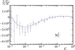
Refer to caption
Refer to caption
Refer to caption
Refer to caption
Refer to caption
Refer to caption
Figure 16: Comparison of the fixed-order analytic SCET prediction for the 𝒪(αs3)𝒪superscriptsubscript𝛼𝑠3\mathcal{O}(\alpha_{s}^{3}) piece with the parton level Monte Carlo EERAD3. The decomposition in the three color structures NC2superscriptsubscript𝑁𝐶2N_{C}^{2}, 111, and NC2superscriptsubscript𝑁𝐶2N_{C}^{-2} are shown in panels (a), (b), and (c), of the first row, respectively, and NCnfsubscript𝑁𝐶subscript𝑛𝑓N_{C}\,n_{f}, nf/NCsubscript𝑛𝑓subscript𝑁𝐶n_{f}/N_{C} and nf2superscriptsubscript𝑛𝑓2n_{f}^{2} are shown in panels (d), (e) and (f), respectively, on the second row. The factor αs3/(2π)3superscriptsubscript𝛼𝑠3superscript2𝜋3\alpha_{s}^{3}/(2\pi)^{3} has been divided out. We use a log binning in the horizontal axis to emphasize the dijet region.
Refer to caption
Refer to caption
Figure 17: Comparison of the determination of the soft function non-logarithmic constants at 𝒪(αs2)𝒪superscriptsubscript𝛼𝑠2{\cal O}(\alpha_{s}^{2}) as explained in Sec. VI (shown as horizontal lines), with a determination employing the method used in Ref. Hoang and Kluth (2008) (plateau at 104C103less-than-or-similar-tosuperscript104𝐶less-than-or-similar-tosuperscript10310^{-4}\lesssim C\lesssim 10^{-3}). The function s2C~(C)superscriptsubscript𝑠2~𝐶𝐶s_{2}^{\widetilde{C}}(C) is defined in Eq. (107). The CFCAsubscript𝐶𝐹subscript𝐶𝐴C_{F}C_{A} and CFnfTfsubscript𝐶𝐹subscript𝑛𝑓subscript𝑇𝑓C_{F}n_{f}T_{f} color structures are shown in left and right panels, respectively. The logarithmic horizontal axis emphasizes the C0𝐶0C\to 0 extrapolation. Error bars are included and the blue and red points correspond to data from a different binning.

At 𝒪(αs3)𝒪superscriptsubscript𝛼𝑠3\mathcal{O}(\alpha_{s}^{3}) we compare to the EERAD3 parton level Monte Carlo output, again splitting the results in the various color structures. Once again we use logarithmically binned distributions for this exercise. The results are shown in Fig. 16. The comparison looks very good for the numerically most relevant color structures (which also have the biggest uncertainties) and quite good for other structures. Slight deviations are observed in some cases for C<103𝐶superscript103C<10^{-3}, presumably indicating systematic uncertainties due the numerical infrared cutoff. The dominant color structures do not have this problem and have larger uncertainties, so one can still use the distribution even for C104similar-to𝐶superscript104C\sim 10^{-4} as long as all color structures are summed up.

In Fig. 17 we compare our numerical determination of s2C~superscriptsubscript𝑠2~𝐶s_{2}^{\widetilde{C}}, that was described above in Sec. VI, to the alternate method used in Ref. Hoang and Kluth (2008) and show that both procedures yield very similar results. The result from Sec. VI is shown as an orange line (whose width is its uncertainty). The method of Ref. Hoang and Kluth (2008) gives the points. In Ref. Hoang and Kluth (2008) s2τsuperscriptsubscript𝑠2𝜏s_{2}^{\tau} is computed from a relation very similar to Eq. (40), written in the following form for C-parameter:

s2C~superscriptsubscript𝑠2~𝐶\displaystyle s_{2}^{\widetilde{C}} =1σ0{σhad(2)Σs(2)(1)|s2C~=0\displaystyle=\dfrac{1}{\sigma_{0}}\bigg{\{}\sigma_{\rm had}^{(2)}-\Sigma_{\rm s}^{(2)}(1)\Big{|}_{s_{2}^{\widetilde{C}}=0} (107)
limC0[Σns(2)(1)Σns(2)(C)]}limC0s2C~(C),\displaystyle-\lim_{C\to 0}\Big{[}\Sigma_{\rm ns}^{(2)}(1)-\Sigma_{\rm ns}^{(2)}(C)\Big{]}\bigg{\}}\equiv\lim_{C\to 0}s_{2}^{\widetilde{C}}(C)\,,

where we have implicitly defined the function s2C~(C)superscriptsubscript𝑠2~𝐶𝐶s_{2}^{\widetilde{C}}(C), and used

Σs,ns(2)(C)superscriptsubscriptΣsns2𝐶\displaystyle\Sigma_{\rm s,ns}^{(2)}(C) =0CdCdσs,ns(2)dC.absentsuperscriptsubscript0𝐶differential-d𝐶dsuperscriptsubscript𝜎sns2d𝐶\displaystyle=\int_{0}^{C}\mathrm{d}C\,\dfrac{\mathrm{d}\sigma_{\rm s,ns}^{(2)}}{\mathrm{d}C}\,. (108)

Eq. (107) can be broken down into various color factors. The limit in Eq. (107) has to be taken numerically from the output of EVENT2. This is best achieved if events are distributed in logarithmic bins, such that the C0𝐶0C\to 0 region is enhanced, as can be seen in Fig. 17. The limit can be identified as the value at which the log-binned distribution reaches a plateau, which in the case of C-parameter happens for 104C103less-than-or-similar-tosuperscript104𝐶less-than-or-similar-tosuperscript10310^{-4}\lesssim C\lesssim 10^{-3}. Figure 17 shows that our determination of s2C~superscriptsubscript𝑠2~𝐶s_{2}^{\widetilde{C}} as described in Sec. VI, represented by an orange line, agrees with the plateau for the two nontrivial color structures.

Appendix C Computation of 1-loop Soft Function

In this section we present a general computation of the 1-loop soft function for any event shape e𝑒e which can be expressed in the dijet limit as

e=1Qipife(yi),𝑒1𝑄subscript𝑖superscriptsubscript𝑝𝑖perpendicular-tosubscript𝑓𝑒subscript𝑦𝑖\displaystyle e=\frac{1}{Q}\sum_{i}p_{i}^{\perp}f_{e}(y_{i})\,, (109)

where the sum is over all particles in the final state, pisubscript𝑝𝑖p_{i} is the magnitude of the transverse momentum and yisubscript𝑦𝑖y_{i} is the rapidity of the particle, both measured with respect to the thrust axis. 777For perturbative computations partons are taken as massless and hence rapidity y𝑦y and pseudorapidity η𝜂\eta coincide. For thrust one has fτ(y)=exp(|y|)subscript𝑓𝜏𝑦𝑦f_{\tau}(y)=\exp(-|y|), for angularities one has fτa(y)=exp[(1a)|y|]subscript𝑓superscript𝜏𝑎𝑦1𝑎𝑦f_{\tau^{a}}(y)=\exp[-(1-a)|y|\,], and for C-parameter one has fC(y)=3/coshysubscript𝑓𝐶𝑦3𝑦f_{C}(y)=3/\cosh y and fC~(y)=1/(2coshy)subscript𝑓~𝐶𝑦12𝑦f_{\widetilde{C}}(y)=1/(2\cosh y).

Refer to caption
Figure 18: Diagrams contributing to the soft function at one loop.

One needs to compute the four diagrams in Fig. 18 in order to determine the soft function. The two diagrams on the bottom are scaleless and vanish in dimensional regularization. They actually convert the IR divergences in the two diagrams on the top into UV divergences. We take the space-time number of dimensions to be d=42ϵ𝑑42italic-ϵd=4-2\epsilon. A direct computation in momentum space gives

Se1loop()=4gs2CFd32ϵp(2π)32ϵ2|p|δ[pTfe(y)]p+p.subscriptsuperscript𝑆1loop𝑒4superscriptsubscript𝑔𝑠2subscript𝐶𝐹superscriptd32italic-ϵ𝑝superscript2𝜋32italic-ϵ2𝑝𝛿delimited-[]subscript𝑝𝑇subscript𝑓𝑒𝑦superscript𝑝superscript𝑝\displaystyle\!\!\!S^{\rm 1-loop}_{e}(\ell)=4\,g_{s}^{2}C_{F}\!\!\int\!\frac{\mathrm{d}^{3-2\epsilon}\vec{p}}{(2\pi)^{3-2\epsilon}2|\vec{p}\,|}\frac{\delta[\ell-p_{T}f_{e}(y)]}{p^{+}p^{-}}\,. (110)

After integrating the angular variables, it is convenient to make a change of variables from p±superscript𝑝plus-or-minusp^{\pm} to (pTsubscript𝑝𝑇p_{T}, y𝑦y):

d32ϵp(2π)32ϵ2|p|=2(4π)2ϵpT12ϵΓ(1ϵ)dpTdy.superscriptd32italic-ϵ𝑝superscript2𝜋32italic-ϵ2𝑝2superscript4𝜋2italic-ϵsuperscriptsubscript𝑝𝑇12italic-ϵΓ1italic-ϵdsubscript𝑝𝑇d𝑦\displaystyle\frac{\mathrm{d}^{3-2\epsilon}{\vec{p}}}{(2\pi)^{3-2\epsilon}2|\vec{p}\,|}=\frac{2}{(4\pi)^{2-\epsilon}}\frac{p_{T}^{1-2\epsilon}}{\Gamma(1-\epsilon)}\,\mathrm{d}p_{T}\mathrm{d}y\,. (111)

Using Eq. (111) in Eq. (110) and imposing the on-shell condition p+p=pT2superscript𝑝superscript𝑝superscriptsubscript𝑝𝑇2p^{+}p^{-}=p_{T}^{2}, where p2=pz2+pT2superscript𝑝2superscriptsubscript𝑝𝑧2superscriptsubscript𝑝𝑇2\vec{p\,}^{2}=p_{z}^{2}+p_{T}^{2}, we obtain

Se1loop()superscriptsubscript𝑆𝑒1loop\displaystyle S_{e}^{\rm 1-loop}(\ell) (112)
=2αs(μ)CFeϵγEμπΓ(1ϵ)dpTdy(pTμ)12ϵδ[pTfe(y)]absent2subscript𝛼𝑠𝜇subscript𝐶𝐹superscript𝑒italic-ϵsubscript𝛾𝐸𝜇𝜋Γ1italic-ϵdifferential-dsubscript𝑝𝑇differential-d𝑦superscriptsubscript𝑝𝑇𝜇12italic-ϵ𝛿delimited-[]subscript𝑝𝑇subscript𝑓𝑒𝑦\displaystyle=\frac{2\,\alpha_{s}(\mu)C_{F}e^{\epsilon\gamma_{E}}}{\mu\,\pi\,\Gamma(1-\epsilon)}\!\int\!\mathrm{d}p_{T}\,\mathrm{d}y\,\Big{(}\frac{p_{T}}{\mu}\Big{)}^{-1-2\epsilon}\delta[\ell-p_{T}f_{e}(y)]
=2αs(μ)CFeϵγEμπΓ(1ϵ)(μ)12ϵIe(ϵ),absent2subscript𝛼𝑠𝜇subscript𝐶𝐹superscript𝑒italic-ϵsubscript𝛾𝐸𝜇𝜋Γ1italic-ϵsuperscript𝜇12italic-ϵsubscript𝐼𝑒italic-ϵ\displaystyle=\frac{2\,\alpha_{s}(\mu)C_{F}e^{\epsilon\gamma_{E}}}{\mu\,\pi\,\Gamma(1-\epsilon)}\Big{(}\frac{\ell}{\mu}\Big{)}^{-1-2\epsilon}\,I_{e}(\epsilon)\,,

where we have defined

Ie(ϵ)=dy[fe(y)]2ϵ.subscript𝐼𝑒italic-ϵsuperscriptsubscriptdifferential-d𝑦superscriptdelimited-[]subscript𝑓𝑒𝑦2italic-ϵ\displaystyle I_{e}(\epsilon)=\int_{-\infty}^{\infty}\!\mathrm{d}y\,[\,f_{e}(y)\,]^{2\epsilon}\,. (113)

Similarly in Fourier space, one gets

S~e1loop(x)=2αsCFπΓ(2ϵ)Γ(1ϵ)(ixμ)2ϵeϵγEIe(ϵ).superscriptsubscript~𝑆𝑒1loop𝑥2subscript𝛼𝑠subscript𝐶𝐹𝜋Γ2italic-ϵΓ1italic-ϵsuperscript𝑖𝑥𝜇2italic-ϵsuperscript𝑒italic-ϵsubscript𝛾𝐸subscript𝐼𝑒italic-ϵ\displaystyle\!\!\!\tilde{S}_{e}^{\rm 1-loop}(x)=\frac{2\,\alpha_{s}C_{F}}{\pi}\frac{\Gamma(-2\epsilon)}{\,\Gamma(1-\epsilon)}(i\,x\,\mu)^{2\epsilon}e^{\epsilon\gamma_{E}}\,I_{e}(\epsilon)\,. (114)

For thrust and angularities, one trivially obtains

Iτ(ϵ)=1ϵ,Iτa(ϵ)=11a1ϵ.formulae-sequencesubscript𝐼𝜏italic-ϵ1italic-ϵsubscript𝐼superscript𝜏𝑎italic-ϵ11𝑎1italic-ϵ\displaystyle I_{\tau}(\epsilon)=\frac{1}{\epsilon}\,,\qquad I_{\tau^{a}}(\epsilon)=\frac{1}{1-a}\frac{1}{\epsilon}\,. (115)

For C-parameter it is convenient to perform a change of variables,

y=12ln(1+x1x),coshy=11x2,formulae-sequence𝑦121𝑥1𝑥𝑦11superscript𝑥2\displaystyle y=\frac{1}{2}\ln\!\Big{(}\frac{1+x}{1-x}\Big{)}\,,\quad\cosh y=\frac{1}{\sqrt{1-x^{2}}}\,, (116)

obtaining for the integral:

IC~(ϵ)subscript𝐼~𝐶italic-ϵ\displaystyle I_{\widetilde{C}}(\epsilon) =212ϵ01dx(1x2)1+ϵ=12Γ(ϵ)2Γ(2ϵ).absentsuperscript212italic-ϵsuperscriptsubscript01differential-d𝑥superscript1superscript𝑥21italic-ϵ12Γsuperscriptitalic-ϵ2Γ2italic-ϵ\displaystyle=2^{1-2\epsilon}\!\int_{0}^{1}\!\mathrm{d}x\,(1-x^{2})^{-1+\epsilon}=\frac{1}{2}\frac{\Gamma(\epsilon)^{2}}{\Gamma(2\epsilon)}\,. (117)

Expanding in ϵ0italic-ϵ0\epsilon\to 0 and upon renormalization in MS¯¯MS{\overline{\rm MS}}, we find for the position space soft function

S~C~1loopsubscriptsuperscript~𝑆1loop~𝐶\displaystyle\tilde{S}^{\rm 1-loop}_{\widetilde{C}} =αs(μ)4πCF[π23+8ln2(ixμeγE)],absentsubscript𝛼𝑠𝜇4𝜋subscript𝐶𝐹delimited-[]superscript𝜋238superscript2𝑖𝑥𝜇superscript𝑒subscript𝛾𝐸\displaystyle=-\frac{\alpha_{s}(\mu)}{4\pi}\,C_{F}\Big{[}\frac{\pi^{2}}{3}+8\ln^{2}(ix\mu e^{\gamma_{E}})\Big{]}\,, (118)
S~τa1loopsubscriptsuperscript~𝑆1loopsuperscript𝜏𝑎\displaystyle\tilde{S}^{\rm 1-loop}_{\tau^{a}} =11aαs(μ)4πCF[π2+8ln2(ixμeγE)].absent11𝑎subscript𝛼𝑠𝜇4𝜋subscript𝐶𝐹delimited-[]superscript𝜋28superscript2𝑖𝑥𝜇superscript𝑒subscript𝛾𝐸\displaystyle=-\frac{1}{1-a}\frac{\alpha_{s}(\mu)}{4\pi}\,C_{F}\Big{[}\pi^{2}+8\ln^{2}(ix\mu e^{\gamma_{E}})\Big{]}\,.

Writing the logarithm of the soft function in Fourier space evaluated at the point x=iexp(γE)/μ𝑥𝑖subscript𝛾𝐸𝜇x=-\,i\exp(-\,\gamma_{E})/\mu in a generic form as

lnS~e=2n=1(αs(μ)4π)nsne.subscript~𝑆𝑒2superscriptsubscript𝑛1superscriptsubscript𝛼𝑠𝜇4𝜋𝑛superscriptsubscript𝑠𝑛𝑒\displaystyle\ln{\widetilde{S}_{e}}=2\sum_{n=1}^{\infty}\Big{(}\frac{\alpha_{s}(\mu)}{4\pi}\Big{)}^{n}s_{n}^{e}\,. (119)

we obtain

s1C~=π26CF,s1τa=11aπ22CF.formulae-sequencesuperscriptsubscript𝑠1~𝐶superscript𝜋26subscript𝐶𝐹superscriptsubscript𝑠1subscript𝜏𝑎11𝑎superscript𝜋22subscript𝐶𝐹\displaystyle s_{1}^{\widetilde{C}}=-\,\frac{\pi^{2}}{6}\,C_{F}\,,\qquad s_{1}^{\tau_{a}}=-\,\frac{1}{1-a}\frac{\pi^{2}}{2}\,C_{F}\,. (120)

Fourier transforming the result, one obtains the renormalized momentum space soft function:

SC~1loopsubscriptsuperscript𝑆1loop~𝐶\displaystyle S^{\rm 1-loop}_{\widetilde{C}} =αs(μ)4πCF(π2δ()16μ[ln(/μ)/μ]+),absentsubscript𝛼𝑠𝜇4𝜋subscript𝐶𝐹superscript𝜋2𝛿16𝜇subscriptdelimited-[]𝜇𝜇\displaystyle=\frac{\alpha_{s}(\mu)}{4\pi}\,C_{F}\bigg{(}\!\pi^{2}\,\delta(\ell)-\frac{16}{\mu}\bigg{[}\frac{\ln(\ell/\mu)}{\ell/\mu}\bigg{]}_{+}\bigg{)}\,, (121)
Sτa1loopsubscriptsuperscript𝑆1loopsubscript𝜏𝑎\displaystyle S^{\rm 1-loop}_{\tau_{a}} =11aαs(μ)4πCF(π23δ()16μ[ln(/μ)/μ]+).absent11𝑎subscript𝛼𝑠𝜇4𝜋subscript𝐶𝐹superscript𝜋23𝛿16𝜇subscriptdelimited-[]𝜇𝜇\displaystyle=\frac{1}{1-a}\frac{\alpha_{s}(\mu)}{4\pi}\,C_{F}\bigg{(}\!\frac{\pi^{2}}{3}\,\delta(\ell)-\frac{16}{\mu}\bigg{[}\frac{\ln(\ell/\mu)}{\ell/\mu}\bigg{]}_{+}\bigg{)}\,.

Appendix D 𝐁𝐢,𝐆𝐢𝐣subscript𝐁𝐢subscript𝐆𝐢𝐣\mathbf{B_{i},G_{ij}} coefficients

The resummed cross section at N3LL can be used to compute various fixed-order coefficients, as in Eqs. (IX.1) and (IX.1). The results for coefficients up to 𝒪(αs3)𝒪superscriptsubscript𝛼𝑠3{\cal O}(\alpha_{s}^{3}) in perturbation theory are summarized here.

The Bisubscript𝐵𝑖B_{i} coefficients read

B1[0]superscriptsubscript𝐵1delimited-[]0\displaystyle B_{1}^{[0]} =CF(2π231),absentsubscript𝐶𝐹2superscript𝜋231\displaystyle=C_{F}\!\left(\dfrac{2\pi^{2}}{3}-1\right), (122)
B2[0]superscriptsubscript𝐵2delimited-[]0\displaystyle B_{2}^{[0]} =CF2( 6ζ3+117π224+11π436)absentsuperscriptsubscript𝐶𝐹26subscript𝜁3117superscript𝜋22411superscript𝜋436\displaystyle=C_{F}^{2}\!\left(-\,6\,\zeta_{3}+1-\frac{17\pi^{2}}{24}+\frac{11\pi^{4}}{36}\right)
+CACF(s2[CFCA]4+283ζ31873π4360+85π224+493324)subscript𝐶𝐴subscript𝐶𝐹superscriptsubscript𝑠2delimited-[]subscript𝐶𝐹subscript𝐶𝐴4283subscript𝜁31873superscript𝜋436085superscript𝜋224493324\displaystyle+C_{A}C_{F}\!\left(\frac{s_{2}^{[C_{F}C_{A}]}}{4}+\frac{283\zeta_{3}}{18}-\frac{73\pi^{4}}{360}+\frac{85\pi^{2}}{24}+\frac{493}{324}\right)
+CFnfTF(s2[nf]422ζ397π26+781),subscript𝐶𝐹subscript𝑛𝑓subscript𝑇𝐹superscriptsubscript𝑠2delimited-[]subscript𝑛𝑓422subscript𝜁397superscript𝜋26781\displaystyle+C_{F}n_{f}T_{F}\!\left(\frac{s_{2}^{[n_{f}]}}{4}-\frac{22\zeta_{3}}{9}-\frac{7\pi^{2}}{6}+\frac{7}{81}\right),
B3[0]superscriptsubscript𝐵3delimited-[]0\displaystyle B_{3}^{[0]} =CA2CF(620179ζ3194441π2ζ32284ζ329217ζ518\displaystyle=C_{A}^{2}C_{F}\!\left(\frac{620179\zeta_{3}}{1944}-\frac{41\pi^{2}\zeta_{3}}{2}-\frac{284\zeta_{3}^{2}}{9}-\frac{217\zeta_{5}}{18}\right.
51082685209952+1294933π2349923641π47776+4471π6102060)\displaystyle\left.-\,\frac{51082685}{209952}+\frac{1294933\pi^{2}}{34992}-\frac{3641\pi^{4}}{7776}+\frac{4471\pi^{6}}{102060}\right)
+CACF2(5π2s2[CFCA]24s2[CFCA]42273ζ59+2ζ323\displaystyle+C_{A}C_{F}^{2}\!\left(\frac{5\pi^{2}s_{2}^{[C_{F}C_{A}]}}{24}-\frac{s_{2}^{[C_{F}C_{A}]}}{4}-\frac{2273\zeta_{5}}{9}+\frac{2\zeta_{3}^{2}}{3}\right.
+248π2ζ3989ζ32714887π668040+23093π419440+172585π23888248superscript𝜋2subscript𝜁3989subscript𝜁32714887superscript𝜋66804023093superscript𝜋419440172585superscript𝜋23888\displaystyle\left.+\,\frac{248\pi^{2}\zeta_{3}}{9}-\frac{89\zeta_{3}}{27}-\frac{14887\pi^{6}}{68040}+\frac{23093\pi^{4}}{19440}+\frac{172585\pi^{2}}{3888}\right.
1850391296)+CACFnfTF(352ζ33+13π2ζ332ζ53\displaystyle\left.-\,\frac{185039}{1296}\right)+C_{A}C_{F}n_{f}T_{F}\!\left(-\frac{352\zeta_{3}}{3}+\frac{13\pi^{2}\zeta_{3}}{3}-\frac{2\zeta_{5}}{3}\right.
+170017113122103903π24374+227π44860)+CF3( 167ζ3\displaystyle\left.+\,\frac{1700171}{13122}-\frac{103903\pi^{2}}{4374}+\frac{227\pi^{4}}{4860}\right)+C_{F}^{3}\bigg{(}-\,167\,\zeta_{3}
+38π2ζ334ζ323+22ζ5467996+139π218109π44038superscript𝜋2subscript𝜁334superscriptsubscript𝜁32322subscript𝜁5467996139superscript𝜋218109superscript𝜋440\displaystyle\left.+\,\frac{38\pi^{2}\zeta_{3}}{3}-\frac{4\zeta_{3}^{2}}{3}+22\zeta_{5}-\frac{4679}{96}+\frac{139\pi^{2}}{18}-\frac{109\pi^{4}}{40}\right.
+42757π6136080)+CF2nfTF(5π2s2[nf]24s2[nf]4+368ζ59\displaystyle\left.+\,\frac{42757\pi^{6}}{136080}\right)+C_{F}^{2}n_{f}T_{F}\!\left(\frac{5\pi^{2}s_{2}^{[n_{f}]}}{24}-\frac{s_{2}^{[n_{f}]}}{4}+\frac{368\zeta_{5}}{9}\right.
94π2ζ39+4324ζ381497π4243035503π21944+112073972)\displaystyle\left.-\,\frac{94\pi^{2}\zeta_{3}}{9}+\frac{4324\zeta_{3}}{81}-\frac{497\pi^{4}}{2430}-\frac{35503\pi^{2}}{1944}+\frac{112073}{972}\right)
+CFnf2TF2(808ζ324319093113122+257π281+52π41215)subscript𝐶𝐹superscriptsubscript𝑛𝑓2superscriptsubscript𝑇𝐹2808subscript𝜁324319093113122257superscript𝜋28152superscript𝜋41215\displaystyle+C_{F}n_{f}^{2}T_{F}^{2}\!\left(\frac{808\zeta_{3}}{243}-\frac{190931}{13122}+\frac{257\pi^{2}}{81}+\frac{52\pi^{4}}{1215}\right)
+j34+s3C~8,subscript𝑗34superscriptsubscript𝑠3~𝐶8\displaystyle+\,\frac{j_{3}}{4}+\frac{s_{3}^{\widetilde{C}}}{8},
B1subscript𝐵1\displaystyle B_{1} =CF(2π2352),absentsubscript𝐶𝐹2superscript𝜋2352\displaystyle=C_{F}\left(\frac{2\pi^{2}}{3}-\frac{5}{2}\right), (123)
B2subscript𝐵2\displaystyle B_{2} =CF2( 6ζ3+41841π224+11π436)absentsuperscriptsubscript𝐶𝐹26subscript𝜁341841superscript𝜋22411superscript𝜋436\displaystyle=C_{F}^{2}\!\left(-\,6\,\zeta_{3}+\frac{41}{8}-\frac{41\pi^{2}}{24}+\frac{11\pi^{4}}{36}\right)
+CACF(s2[CFCA]4+481ζ31873π4360+85π2248977648)subscript𝐶𝐴subscript𝐶𝐹superscriptsubscript𝑠2delimited-[]subscript𝐶𝐹subscript𝐶𝐴4481subscript𝜁31873superscript𝜋436085superscript𝜋2248977648\displaystyle+C_{A}C_{F}\!\left(\frac{s_{2}^{[C_{F}C_{A}]}}{4}+\frac{481\zeta_{3}}{18}-\frac{73\pi^{4}}{360}+\frac{85\pi^{2}}{24}-\frac{8977}{648}\right)
+CFnfTF(s2[nf]458ζ397π26+905162),subscript𝐶𝐹subscript𝑛𝑓subscript𝑇𝐹superscriptsubscript𝑠2delimited-[]subscript𝑛𝑓458subscript𝜁397superscript𝜋26905162\displaystyle+C_{F}n_{f}T_{F}\!\left(\frac{s_{2}^{[n_{f}]}}{4}-\frac{58\zeta_{3}}{9}-\frac{7\pi^{2}}{6}+\frac{905}{162}\right),
B3subscript𝐵3\displaystyle B_{3} =CA2CF(915775ζ3194441π2ζ32284ζ329+113ζ518\displaystyle=C_{A}^{2}C_{F}\!\left(\frac{915775\zeta_{3}}{1944}-\frac{41\pi^{2}\zeta_{3}}{2}-\frac{284\zeta_{3}^{2}}{9}+\frac{113\zeta_{5}}{18}\right.
95038955209952+1353739π2349923641π47776+4471π6102060)\displaystyle\left.-\,\frac{95038955}{209952}+\frac{1353739\pi^{2}}{34992}-\frac{3641\pi^{4}}{7776}+\frac{4471\pi^{6}}{102060}\right)
+CACF2(5π2s2[CFCA]245s2[CFCA]83263ζ59+2ζ323\displaystyle+C_{A}C_{F}^{2}\!\left(\frac{5\pi^{2}s_{2}^{[C_{F}C_{A}]}}{24}-\frac{5s_{2}^{[C_{F}C_{A}]}}{8}-\frac{3263\zeta_{5}}{9}+\frac{2\zeta_{3}^{2}}{3}\right.
+314π2ζ39+67ζ310814887π668040+14503π49720+56039π21944314superscript𝜋2subscript𝜁3967subscript𝜁310814887superscript𝜋66804014503superscript𝜋4972056039superscript𝜋21944\displaystyle\left.+\,\frac{314\pi^{2}\zeta_{3}}{9}+\frac{67\zeta_{3}}{108}-\frac{14887\pi^{6}}{68040}+\frac{14503\pi^{4}}{9720}+\frac{56039\pi^{2}}{1944}\right.
877191296)+CACFnfTF(1952ζ39+13π2ζ3322ζ53\displaystyle\left.-\,\frac{87719}{1296}\right)+C_{A}C_{F}n_{f}T_{F}\!\left(-\,\frac{1952\zeta_{3}}{9}+\frac{13\pi^{2}\zeta_{3}}{3}-\frac{22\zeta_{5}}{3}\right.
+358585113122109249π24374+227π44860)+CF3( 158ζ3\displaystyle\left.+\,\frac{3585851}{13122}-\frac{109249\pi^{2}}{4374}+\frac{227\pi^{4}}{4860}\right)+C_{F}^{3}\bigg{(}-\,158\,\zeta_{3}
+38π2ζ334ζ323+22ζ5509396+1517π2144191π46038superscript𝜋2subscript𝜁334superscriptsubscript𝜁32322subscript𝜁55093961517superscript𝜋2144191superscript𝜋460\displaystyle\left.+\,\frac{38\pi^{2}\zeta_{3}}{3}-\frac{4\zeta_{3}^{2}}{3}+22\,\zeta_{5}-\frac{5093}{96}+\frac{1517\pi^{2}}{144}-\frac{191\pi^{4}}{60}\right.
+42757π6136080)+CF2nfTF(5π2s2[nf]245s2[nf]8+728ζ59\displaystyle\left.+\,\frac{42757\pi^{6}}{136080}\right)+C_{F}^{2}n_{f}T_{F}\!\left(\frac{5\pi^{2}s_{2}^{[n_{f}]}}{24}-\frac{5s_{2}^{[n_{f}]}}{8}+\frac{728\zeta_{5}}{9}\right.
118π2ζ39+2839ζ381497π4243024973π21944+1881731944)\displaystyle\left.-\,\frac{118\pi^{2}\zeta_{3}}{9}+\frac{2839\zeta_{3}}{81}-\frac{497\pi^{4}}{2430}-\frac{24973\pi^{2}}{1944}+\frac{188173}{1944}\right)
+CFnf2TF2(4912ζ324348447513122+275π281+52π41215)subscript𝐶𝐹superscriptsubscript𝑛𝑓2superscriptsubscript𝑇𝐹24912subscript𝜁324348447513122275superscript𝜋28152superscript𝜋41215\displaystyle+C_{F}n_{f}^{2}T_{F}^{2}\!\left(\frac{4912\zeta_{3}}{243}-\frac{484475}{13122}+\frac{275\pi^{2}}{81}+\frac{52\pi^{4}}{1215}\right)
+j34+s3C~8.subscript𝑗34superscriptsubscript𝑠3~𝐶8\displaystyle+\,\frac{j_{3}}{4}+\frac{s_{3}^{\widetilde{C}}}{8}.

The results for the first few Gijsubscript𝐺𝑖𝑗G_{ij} coefficients read

G12=subscript𝐺12absent\displaystyle G_{12}= 2CF,G11=3CF,2subscript𝐶𝐹subscript𝐺113subscript𝐶𝐹\displaystyle-2\,C_{F},\>\>\>\>G_{11}=3\,C_{F}, (124)
G23=subscript𝐺23absent\displaystyle G_{23}= CF(4nfTF311CA3),subscript𝐶𝐹4subscript𝑛𝑓subscript𝑇𝐹311subscript𝐶𝐴3\displaystyle\,C_{F}\!\left(\frac{4n_{f}T_{F}}{3}-\frac{11C_{A}}{3}\right),
G22=subscript𝐺22absent\displaystyle G_{22}= CF[CA(π2316936)43π2CF+11nfTF9],subscript𝐶𝐹delimited-[]subscript𝐶𝐴superscript𝜋231693643superscript𝜋2subscript𝐶𝐹11subscript𝑛𝑓subscript𝑇𝐹9\displaystyle C_{F}\!\left[C_{A}\!\left(\frac{\pi^{2}}{3}-\frac{169}{36}\right)-\frac{4}{3}\pi^{2}C_{F}+\frac{11n_{f}T_{F}}{9}\right],
G21=subscript𝐺21absent\displaystyle G_{21}= CF[CA( 6ζ3+574+11π29)\displaystyle\,C_{F}\!\left[C_{A}\!\left(-\,6\,\zeta_{3}+\frac{57}{4}+\frac{11\pi^{2}}{9}\right)\right.
+CF( 4ζ3+34+π2)+nfTF( 54π29)],\displaystyle\left.+\,C_{F}\!\left(-\,4\,\zeta_{3}+\frac{3}{4}+\pi^{2}\right)+n_{f}T_{F}\!\left(-\,5-\frac{4\pi^{2}}{9}\right)\right],
G34=subscript𝐺34absent\displaystyle G_{34}= CF(847CA2108+15427CAnfTF2827nf2TF2),subscript𝐶𝐹847superscriptsubscript𝐶𝐴210815427subscript𝐶𝐴subscript𝑛𝑓subscript𝑇𝐹2827superscriptsubscript𝑛𝑓2superscriptsubscript𝑇𝐹2\displaystyle\,C_{F}\!\left(-\,\frac{847C_{A}^{2}}{108}+\frac{154}{27}C_{A}n_{f}T_{F}-\frac{28}{27}n_{f}^{2}T_{F}^{2}\right),
G33=subscript𝐺33absent\displaystyle G_{33}= CF[CA2(11π293197108)22π23CACF\displaystyle\,C_{F}\!\left[C_{A}^{2}\!\left(\frac{11\pi^{2}}{9}-\frac{3197}{108}\right)-\frac{22\pi^{2}}{3}C_{A}C_{F}\right.
+CAnfTF(512274π29)+64CF2ζ33subscript𝐶𝐴subscript𝑛𝑓subscript𝑇𝐹512274superscript𝜋2964superscriptsubscript𝐶𝐹2subscript𝜁33\displaystyle+C_{A}n_{f}T_{F}\!\left(\frac{512}{27}-\frac{4\pi^{2}}{9}\right)+\frac{64C_{F}^{2}\zeta_{3}}{3}
+CFnfTF(2+8π23)6827nf2TF2],\displaystyle\left.+\,C_{F}n_{f}T_{F}\!\left(2+\frac{8\pi^{2}}{3}\right)-\frac{68}{27}n_{f}^{2}T_{F}^{2}\right],
G32=subscript𝐺32absent\displaystyle G_{32}= CF[CA2(11ζ311323648+497π25411π490)\displaystyle\,C_{F}\!\left[C_{A}^{2}\!\left(11\,\zeta_{3}-\frac{11323}{648}+\frac{497\pi^{2}}{54}-\frac{11\pi^{4}}{90}\right)\right.
+CACF( 110ζ3+11870π227+4π49)subscript𝐶𝐴subscript𝐶𝐹110subscript𝜁311870superscript𝜋2274superscript𝜋49\displaystyle+C_{A}C_{F}\!\left(-\,110\,\zeta_{3}+\frac{11}{8}-\frac{70\pi^{2}}{27}+\frac{4\pi^{4}}{9}\right)
+CAnfTF(4ζ3+673162152π227)subscript𝐶𝐴subscript𝑛𝑓subscript𝑇𝐹4subscript𝜁3673162152superscript𝜋227\displaystyle+C_{A}n_{f}T_{F}\!\left(4\,\zeta_{3}+\frac{673}{162}-\frac{152\pi^{2}}{27}\right)
+CF2(8π44548ζ3)+CFnfTF(32ζ3+436+8π227)superscriptsubscript𝐶𝐹28superscript𝜋44548subscript𝜁3subscript𝐶𝐹subscript𝑛𝑓subscript𝑇𝐹32subscript𝜁34368superscript𝜋227\displaystyle+C_{F}^{2}\!\left(\frac{8\pi^{4}}{45}-48\zeta_{3}\right)+C_{F}n_{f}T_{F}\!\left(32\,\zeta_{3}+\frac{43}{6}+\frac{8\pi^{2}}{27}\right)
+nf2TF2(7081+8π29)],\displaystyle\left.+\,n_{f}^{2}T_{F}^{2}\!\left(\frac{70}{81}+\frac{8\pi^{2}}{9}\right)\right],
G31=subscript𝐺31absent\displaystyle G_{31}= CA2CF(11s2[CFCA]6+10ζ5361ζ327541π4540+892π281\displaystyle\,C_{A}^{2}C_{F}\!\left(\frac{11s_{2}^{[C_{F}C_{A}]}}{6}+10\,\zeta_{5}-\frac{361\zeta_{3}}{27}-\frac{541\pi^{4}}{540}+\frac{892\pi^{2}}{81}\right.
+77099486)+CACF2(452ζ39+2π2ζ3+30ζ5+232\displaystyle\left.+\,\frac{77099}{486}\right)+C_{A}C_{F}^{2}\!\left(\frac{452\zeta_{3}}{9}+2\pi^{2}\zeta_{3}+30\,\zeta_{5}+\frac{23}{2}\right.
+161π27249π4135)+CACFnfTF(2s2[CFCA]3\displaystyle\left.+\,\frac{161\pi^{2}}{72}-\frac{49\pi^{4}}{135}\right)+C_{A}C_{F}n_{f}T_{F}\!\left(-\,\frac{2s_{2}^{[C_{F}C_{A}]}}{3}\right.
+11s2[nf]6608ζ327+10π427520π28124844243)\displaystyle\left.+\,\frac{11s_{2}^{[n_{f}]}}{6}-\frac{608\zeta_{3}}{27}+\frac{10\pi^{4}}{27}-\frac{520\pi^{2}}{81}-\frac{24844}{243}\right)
+CF3(53ζ344π2ζ33+132ζ5+298+5π248π415)superscriptsubscript𝐶𝐹353subscript𝜁344superscript𝜋2subscript𝜁33132subscript𝜁52985superscript𝜋248superscript𝜋415\displaystyle+C_{F}^{3}\!\left(53\,\zeta_{3}-\frac{44\pi^{2}\zeta_{3}}{3}+132\zeta_{5}+\frac{29}{8}+\frac{5\pi^{2}}{4}-\frac{8\pi^{4}}{15}\right)
+CF2nfTF(208ζ3977431π218+8π4135)superscriptsubscript𝐶𝐹2subscript𝑛𝑓subscript𝑇𝐹208subscript𝜁3977431superscript𝜋2188superscript𝜋4135\displaystyle+C_{F}^{2}n_{f}T_{F}\!\left(-\,\frac{208\zeta_{3}}{9}-\frac{77}{4}-\frac{31\pi^{2}}{18}+\frac{8\pi^{4}}{135}\right)
+CFnf2TF2(2s2[nf]3+176ζ327+64π281+3598243).subscript𝐶𝐹superscriptsubscript𝑛𝑓2superscriptsubscript𝑇𝐹22superscriptsubscript𝑠2delimited-[]subscript𝑛𝑓3176subscript𝜁32764superscript𝜋2813598243\displaystyle+C_{F}n_{f}^{2}T_{F}^{2}\!\left(\!-\,\frac{2s_{2}^{[n_{f}]}}{3}+\frac{176\zeta_{3}}{27}+\frac{64\pi^{2}}{81}+\frac{3598}{243}\right).

Note that the entire infinite series of Gijsubscript𝐺𝑖𝑗G_{ij} coefficients listed in Table 4 is determined by our resummation results.

Appendix E R-evolution with and without Hadron Mass Effects

The result for R-evolution in the case of no hadron masses is given in Eq. (VII). The resummed ω𝜔\omega appearing in this equation was given in App. A. The remaining coefficients and variables that appear in this equation are

S0subscript𝑆0\displaystyle S_{0} =γ0R2β0,S1=γ1R(2β0)2(b^1+b^2)γ0R2β0,formulae-sequenceabsentsuperscriptsubscript𝛾0𝑅2subscript𝛽0subscript𝑆1superscriptsubscript𝛾1𝑅superscript2subscript𝛽02subscript^𝑏1subscript^𝑏2superscriptsubscript𝛾0𝑅2subscript𝛽0\displaystyle=\frac{\gamma_{0}^{R}}{2\beta_{0}}\,,\,\,S_{1}=\frac{\gamma_{1}^{R}}{(2\beta_{0})^{2}}-(\hat{b}_{1}+\hat{b}_{2})\frac{\gamma_{0}^{R}}{2\beta_{0}}\,,
S2subscript𝑆2\displaystyle S_{2} =γ2R(2β0)3(b^1+b^2)γ1R(2β0)2,absentsuperscriptsubscript𝛾2𝑅superscript2subscript𝛽03subscript^𝑏1subscript^𝑏2superscriptsubscript𝛾1𝑅superscript2subscript𝛽02\displaystyle=\frac{\gamma_{2}^{R}}{(2\beta_{0})^{3}}-(\hat{b}_{1}+\hat{b}_{2})\frac{\gamma_{1}^{R}}{(2\beta_{0})^{2}}\,,
b^1subscript^𝑏1\displaystyle\hat{b}_{1} =β12β02,b^2=β12β0β24β04,formulae-sequenceabsentsubscript𝛽12superscriptsubscript𝛽02subscript^𝑏2superscriptsubscript𝛽12subscript𝛽0subscript𝛽24superscriptsubscript𝛽04\displaystyle=\frac{\beta_{1}}{2\beta_{0}^{2}}\,,\;\;\hat{b}_{2}=\frac{\beta_{1}^{2}-\beta_{0}\beta_{2}}{4\beta_{0}^{4}}\,, (125)
b^3subscript^𝑏3\displaystyle\hat{b}_{3} =β132β0β1β2+β02β38β06,absentsuperscriptsubscript𝛽132subscript𝛽0subscript𝛽1subscript𝛽2superscriptsubscript𝛽02subscript𝛽38superscriptsubscript𝛽06\displaystyle=\frac{\beta_{1}^{3}-2\beta_{0}\beta_{1}\beta_{2}+\beta_{0}^{2}\beta_{3}}{8\beta_{0}^{6}}\,,
t1subscript𝑡1\displaystyle t_{1} =2πβ0αs(R),t0=2πβ0αs(RΔ).formulae-sequenceabsent2𝜋subscript𝛽0subscript𝛼𝑠𝑅subscript𝑡02𝜋subscript𝛽0subscript𝛼𝑠subscript𝑅Δ\displaystyle=-\,\frac{2\pi}{\beta_{0}\alpha_{s}(R)},\,t_{0}=-\,\frac{2\pi}{\beta_{0}\alpha_{s}(R_{\Delta})}\,.
Refer to caption
Figure 19: Running of the short-distance power correction Ω1h(R,R,h)superscriptsubscriptΩ1𝑅𝑅\Omega_{1}^{h}(R,R,h) with respect to the reference value Ω1h(RΔ,RΔ,1)superscriptsubscriptΩ1subscript𝑅Δsubscript𝑅Δ1\Omega_{1}^{h}(R_{\Delta},R_{\Delta},1). The scale R𝑅R is set to the default profile, and the scheme parameter hh is set to the function displayed in Eq. (141). Red , blue, and green correspond to center-of-mass energies of 91.291.291.2, 404040, and 200200200 GeV, respectively. The solid lines do not include hadron-mass effects, whereas the dashed ones do.

The impact of R-evolution on the value of the hadronic parameter Ω1(R,R)subscriptΩ1𝑅𝑅\Omega_{1}(R,R) is shown in Fig. 19 (with and without hadron-mass effects). Here we have set μ=R𝜇𝑅\mu=R and used the default profile function for R(C)𝑅𝐶R(C). We actually plot the hybrid scheme Ω1h(R,R,h)superscriptsubscriptΩ1𝑅𝑅\Omega_{1}^{h}(R,R,h) which accounts for a reasonable treatment of threshold effects at the shoulder C=0.75𝐶0.75C=0.75 and which is discussed in detail below in App. F. The effect of using the hybrid scheme rather than the Rgap scheme is quite small in the region of this figure but does cause the bending over of the curves that is visible at C=0.6𝐶0.6C=0.6. Above the shoulder the hybrid scheme uses the MS¯¯MS\overline{\textrm{MS}} power correction, which has a flat behavior.

When we introduce hadron-mass effects, it is necessary to extent these results to account for the value of r𝑟r, the transverse velocity. Due to the running in Eq. (66), the scheme change result in Eq. (51) now becomes

gC(r)Ω1C(R,μ,r)subscript𝑔𝐶𝑟superscriptsubscriptΩ1𝐶𝑅𝜇𝑟\displaystyle g_{C}(r)\,\Omega_{1}^{C}(R,\mu,r) =gC(r)Ω¯1(μ,r)δ(R,μ,r),absentsubscript𝑔𝐶𝑟subscript¯Ω1𝜇𝑟𝛿𝑅𝜇𝑟\displaystyle=g_{C}(r)\,\overline{\Omega}_{1}(\mu,r)-\delta(R,\mu,r)\,, (126)

where there is additional μ𝜇\mu dependence from the hadron-mass induced running. Our scheme for δ𝛿\delta now becomes

δ(R,μ,r)𝛿𝑅𝜇𝑟\displaystyle\delta(R,\mu,r) =[αs(μ)αs(R)]γ^1(r)δ(R,μ),absentsuperscriptdelimited-[]subscript𝛼𝑠𝜇subscript𝛼𝑠𝑅subscript^𝛾1𝑟𝛿𝑅𝜇\displaystyle=\left[\frac{\alpha_{s}(\mu)}{\alpha_{s}(R)}\right]^{\hat{\gamma}_{1}(r)}\!\delta(R,\mu)\,, (127)

and the r𝑟r dependence is encoded in the known one-loop anomalous dimension Mateu et al. (2013)

γ^1(r)subscript^𝛾1𝑟\displaystyle\hat{\gamma}_{1}(r) =2CAβ0ln(1r2).absent2subscript𝐶𝐴subscript𝛽01superscript𝑟2\displaystyle=\frac{2\,C_{\!A}}{\beta_{0}}\ln(1-r^{2})\,. (128)

With this r𝑟r-dependent scheme change, we can once again derive the equations that govern the R𝑅R evolution and μ𝜇\mu running for Ω1CsuperscriptsubscriptΩ1𝐶\Omega_{1}^{C}, which following Ref. Hoang et al. (2015c) become

RddR{[gC(r)Ω1C(R,μ,r)(αs(μ))γ^1(r)]μ=R}𝑅dd𝑅subscriptdelimited-[]subscript𝑔𝐶𝑟superscriptsubscriptΩ1𝐶𝑅𝜇𝑟superscriptsubscript𝛼𝑠𝜇subscript^𝛾1𝑟𝜇𝑅\displaystyle R\frac{\mathrm{d}}{\mathrm{d}R}\Big{\{}\Big{[}g_{C}(r)\,\Omega_{1}^{C}(R,\mu,r)\big{(}\alpha_{s}(\mu)\big{)}^{-\hat{\gamma}_{1}(r)}\Big{]}_{\mu=R}\Big{\}} (129)
=R(αs(R))γ^1(r)n=0γnRr(r)(αs(R)4π)n+1,absent𝑅superscriptsubscript𝛼𝑠𝑅subscript^𝛾1𝑟superscriptsubscript𝑛0superscriptsubscript𝛾𝑛𝑅𝑟𝑟superscriptsubscript𝛼𝑠𝑅4𝜋𝑛1\displaystyle\quad=-\,R\,\big{(}\alpha_{s}(R)\big{)}^{-\hat{\gamma}_{1}(r)}\sum_{n=0}^{\infty}\gamma_{n}^{R\,r}(r)\left(\frac{\alpha_{s}(R)}{4\pi}\right)^{\!\!n+1}\,,
μddμ{gC(r)Ω1C(R,μ,r)(αs(μ))γ^1(r)}𝜇dd𝜇subscript𝑔𝐶𝑟superscriptsubscriptΩ1𝐶𝑅𝜇𝑟superscriptsubscript𝛼𝑠𝜇subscript^𝛾1𝑟\displaystyle\mu\frac{\mathrm{d}}{\mathrm{d}\mu}\Big{\{}g_{C}(r)\,\Omega_{1}^{C}(R,\mu,r)\big{(}\alpha_{s}(\mu)\big{)}^{-\hat{\gamma}_{1}(r)}\Big{\}}
=2ReγE(αs(R))γ^1(r)n=0Γncusp(αs(μ)4π)n+1,absent2𝑅superscript𝑒subscript𝛾𝐸superscriptsubscript𝛼𝑠𝑅subscript^𝛾1𝑟superscriptsubscript𝑛0superscriptsubscriptΓ𝑛cuspsuperscriptsubscript𝛼𝑠𝜇4𝜋𝑛1\displaystyle\quad=2\,R\,e^{\gamma_{E}}\big{(}\alpha_{s}(R)\big{)}^{-\hat{\gamma}_{1}(r)}\sum_{n=0}^{\infty}\Gamma_{n}^{\text{cusp}}\left(\frac{\alpha_{s}(\mu)}{4\pi}\right)^{\!\!n+1},

for

γ0Rr(r)superscriptsubscript𝛾0𝑅𝑟𝑟\displaystyle\gamma_{0}^{R\,r}(r) =γ0R,γ1Rr(r)=γ1R+2β0γ^1(r)γ0R,formulae-sequenceabsentsuperscriptsubscript𝛾0𝑅superscriptsubscript𝛾1𝑅𝑟𝑟superscriptsubscript𝛾1𝑅2subscript𝛽0subscript^𝛾1𝑟superscriptsubscript𝛾0𝑅\displaystyle=\gamma_{0}^{R},\qquad\gamma_{1}^{R\,r}(r)=\gamma_{1}^{R}+2\beta_{0}\hat{\gamma}_{1}(r)\gamma_{0}^{R}\,,
γ2Rr(r)superscriptsubscript𝛾2𝑅𝑟𝑟\displaystyle\gamma_{2}^{R\,r}(r) =γ2R+2β0γ^1(r)(γ1R+2β0γ0R).absentsuperscriptsubscript𝛾2𝑅2subscript𝛽0subscript^𝛾1𝑟superscriptsubscript𝛾1𝑅2subscript𝛽0superscriptsubscript𝛾0𝑅\displaystyle=\gamma_{2}^{R}+2\beta_{0}\hat{\gamma}_{1}(r)(\gamma_{1}^{R}+2\beta_{0}\gamma_{0}^{R})\,. (130)

Solving this set of equations gives Eq. (VII.1), with the Sirsuperscriptsubscript𝑆𝑖𝑟S_{i}^{r} given by

S0r(r)subscriptsuperscript𝑆𝑟0𝑟\displaystyle S^{r}_{0}(r) =S0,S1r(r)=S1+γ^1(r)γ0R2β0,formulae-sequenceabsentsubscript𝑆0subscriptsuperscript𝑆𝑟1𝑟subscript𝑆1subscript^𝛾1𝑟superscriptsubscript𝛾0𝑅2subscript𝛽0\displaystyle=S_{0}\,,\qquad S^{r}_{1}(r)=S_{1}+\frac{\hat{\gamma}_{1}(r)\gamma_{0}^{R}}{2\beta_{0}}\,, (131)
S2r(r)subscriptsuperscript𝑆𝑟2𝑟\displaystyle S^{r}_{2}(r) =S2+(γ1R+2β0γ0R)absentsubscript𝑆2superscriptsubscript𝛾1𝑅2subscript𝛽0superscriptsubscript𝛾0𝑅\displaystyle=S_{2}+(\gamma_{1}^{R}+2\beta_{0}\gamma_{0}^{R})
×[(1+b^1)b^2+b^22+b^32]γ^1(r)(2β0)2.absentdelimited-[]1subscript^𝑏1subscript^𝑏2superscriptsubscript^𝑏22subscript^𝑏32subscript^𝛾1𝑟superscript2subscript𝛽02\displaystyle\ \ \times\bigg{[}(1+\hat{b}_{1})\,\hat{b}_{2}+\frac{\hat{b}_{2}^{2}+\hat{b}_{3}}{2}\bigg{]}\frac{\hat{\gamma}_{1}(r)}{(2\beta_{0})^{2}}\,.

Values for the γiRsuperscriptsubscript𝛾𝑖𝑅\gamma_{i}^{R} anomalous dimensions were given above in Eq. (55).

Appendix F Gap Scheme in the Fixed-Order Region

In the fixed-order (or far-tail) region, there is no longer a hierarchy between the hard, jet, and soft scales, and one sets them equal to reproduce the fixed-order QCD predictions exactly. This is done through our profiles. In this region the singular and non-singular terms are of similar size, and hence the factorization of the cross section in a hard factor and a convolution of jet and soft functions is no longer relevant. The issue is further complicated by the analytic structure of the shoulder region, which is located in the fixed-order region and contains the integrable singularity at C=0.75𝐶0.75C=0.75 which has its own logarithmic series (see Fig. 5 and the accompanying discussion there). Thus, in the far-tail region C0.75greater-than-or-equivalent-to𝐶0.75C\gtrsim 0.75, the structure of nonperturbative corrections is likely to differ from that of the shape function FCsubscript𝐹𝐶F_{C} and thus is unknown at this time. Nevertheless, we do expect a smearing by a function whose width is ΛQCDsimilar-toabsentsubscriptΛQCD\sim\Lambda_{\rm QCD}, and hence our smearing by FCsubscript𝐹𝐶F_{C} is simply a proxy for a more detailed analysis in this region. Since fits for αssubscript𝛼𝑠\alpha_{s} can be carried out with C<0.75𝐶0.75C<0.75, the treatment of this region, and the discussion below, are not relevant for predicting the shape in the fit region. The region C0.75𝐶0.75C\geq 0.75 does contribute when computing the total cross section from our resummed result, and this motivates us to use a cross section formula that still obtains realistic results in this region.

Due to the shoulder at C=0.75𝐶0.75C=0.75, the use of the infrared subtractions δ𝛿\delta in this region can cause an unphysical behavior of the cross section. The reason for this is that these subtractions yield derivatives acting on the partonic cross section. In the shoulder region with the singular discontinuity starting at 𝒪(αs2)𝒪superscriptsubscript𝛼𝑠2\mathcal{O}(\alpha_{s}^{2}), these derivatives can cause an artificially enhanced singular behavior if the subtraction is not carefully defined in this region. If this is not done, the convolution with the shape function FCsubscript𝐹𝐶F_{C} may be insufficient to achieve a smooth cross section near C0.75similar-to-or-equals𝐶0.75C\simeq 0.75. In Ref. Catani and Webber (1998) it was shown that the singularities at C=0.75𝐶0.75C=0.75 can be cured by including soft gluon resummation which makes the cross section smooth. However, this treatment does not resolve the question of the proper field theoretic nonperturbative function for this region, nor any accompanying infrared subtractions due to renormalons.

To deal with the region C0.75greater-than-or-equivalent-to𝐶0.75C\gtrsim 0.75 we take an alternative approach, which is to implement a smooth transition between the Rgap scheme in the dijet region to MS¯¯MS\overline{\textrm{MS}} in the fixed-order region. This avoids any subtractions at C=0.75𝐶0.75C=0.75. To that end we define a new scheme that depends on a continuous parameter hh which takes values between 00 and 111 and that smoothly switches off the gap subtractions when we get near C=0.75𝐶0.75C=0.75. We start by rewriting Eq. (47) as

ΔCsubscriptΔ𝐶\displaystyle\Delta_{C} =3π2[Δ¯h(R,μ,h)+hδ(R,μ)].absent3𝜋2delimited-[]superscript¯Δ𝑅𝜇𝛿𝑅𝜇\displaystyle=\frac{3\pi}{2}[\,\bar{\Delta}^{h}(R,\mu,h)+h\,\delta(R,\mu)\,]\,. (132)

This defines a hybrid short-distance scheme for Ω1subscriptΩ1\Omega_{1} which we call Ω1hsuperscriptsubscriptΩ1\Omega_{1}^{h},

Ω1h(R,μ,h)superscriptsubscriptΩ1𝑅𝜇\displaystyle\Omega_{1}^{h}(R,\mu,h) =Ω¯1C3πhδ(R,μ),absentsuperscriptsubscript¯Ω1𝐶3𝜋𝛿𝑅𝜇\displaystyle=\overline{\Omega}_{1}^{C}-3\pi\,h\,\delta(R,\mu)\,, (133)

which becomes the MS¯¯MS\overline{\textrm{MS}} scheme for h=00h=0 and the Rgap scheme for h=11h=1. One can easily derive RGE equations in μ𝜇\mu and R𝑅R, for Δ¯hsuperscript¯Δ\bar{\Delta}^{h}, which we write in the convenient form 888The right-hand sides of the running equations for the power correction Ω1h(R,μS,h)superscriptsubscriptΩ1𝑅subscript𝜇𝑆\Omega_{1}^{h}(R,\mu_{S},h) are simply 3π3𝜋3\pi times the right-hand sides of Eqs. (134) and (135).

RddRΔ¯h(R,R,h)𝑅dd𝑅superscript¯Δ𝑅𝑅\displaystyle R\frac{\mathrm{d}}{\mathrm{d}R}\bar{\Delta}^{h}(R,R,h) =hRγR[αs(R)],absent𝑅superscript𝛾𝑅delimited-[]subscript𝛼𝑠𝑅\displaystyle=-\,h\,R\,\gamma^{R}[\alpha_{s}(R)]\,, (134)
μddμΔ¯h(R,μ,h)𝜇dd𝜇superscript¯Δ𝑅𝜇\displaystyle\mu\frac{\mathrm{d}}{\mathrm{d}\mu}\bar{\Delta}^{h}(R,\mu,h) =2RheγEΓcusp[αs(μ)],absent2𝑅superscript𝑒subscript𝛾𝐸subscriptΓcuspdelimited-[]subscript𝛼𝑠𝜇\displaystyle=2\,R\,h\,e^{\gamma_{E}}\Gamma_{\rm cusp}[\alpha_{s}(\mu)]\,,

and a relation to switch from different hh schemes:

Δ¯h(R,μ,h1)Δ¯h(R,μ,h2)=(h2h1)δ(R,μ).superscript¯Δ𝑅𝜇subscript1superscript¯Δ𝑅𝜇subscript2subscript2subscript1𝛿𝑅𝜇\displaystyle\bar{\Delta}^{h}(R,\mu,h_{1})-\bar{\Delta}^{h}(R,\mu,h_{2})=(h_{2}-h_{1})\,\delta(R,\mu)\,. (135)

The solution to these three equations is rather simple,

Δ¯h(R,μ,h)superscript¯Δ𝑅𝜇\displaystyle\bar{\Delta}^{h}(R,\mu,h) =Δ¯h(RΔ,μΔ,hΔ)(hhΔ)δ(R,μ)absentsuperscript¯Δsubscript𝑅Δsubscript𝜇ΔsubscriptΔsubscriptΔ𝛿𝑅𝜇\displaystyle=\bar{\Delta}^{h}(R_{\Delta},\mu_{\Delta},h_{\Delta})-(h-h_{\Delta})\delta(R,\mu)
+hΔΔdiff(RΔ,R,μΔ,μ),subscriptΔsuperscriptΔdiffsubscript𝑅Δ𝑅subscript𝜇Δ𝜇\displaystyle+h_{\Delta}\,\Delta^{\rm diff}(R_{\Delta},R,\mu_{\Delta},\mu)\,, (136)

where ΔdiffsuperscriptΔdiff\Delta^{\rm diff} has been defined in Eq. (VII). We choose to evolve first in R𝑅R and μ𝜇\mu in the hΔsubscriptΔh_{\Delta} scheme, where above the peak region [see Eq. (78)] there is only a single evolution since μS(C)=R(C)subscript𝜇𝑆𝐶𝑅𝐶\mu_{S}(C)=R(C). Close to the shoulder region C0.75similar-to𝐶0.75C\sim 0.75, we then smoothly transform from the hΔsubscriptΔh_{\Delta} scheme to the hh scheme. This implements the transition from the Rgap scheme with 𝒪(ΛQCD)𝒪subscriptΛQCD{\cal O}(\Lambda_{\rm QCD}) renormalon subtraction to the MS¯¯MS\overline{\textrm{MS}} scheme where this renormalon is not subtracted. The procedure entails a residual dependence on R𝑅R in the region C0.75greater-than-or-equivalent-to𝐶0.75C\gtrsim 0.75 even once h=00h=0, which comes from the fact that we are transforming from Rgap to MS¯¯MS\overline{\textrm{MS}} at the scale R>RΔ𝑅subscript𝑅ΔR>R_{\Delta}. This residual dependence leads to a somewhat smaller effect of the 𝒪(ΛQCD)𝒪subscriptΛQCD{\cal O}(\Lambda_{\rm QCD}) renormalon even though one employs Ω¯1subscript¯Ω1\overline{\Omega}_{1} in this region.

In the hybrid scheme described above, the first moment of the shape function reads

dkkFC(k)=Ω1h(RΔ,μΔ,hΔ) 3πΔ¯h(RΔ,μΔ,hΔ).differential-d𝑘𝑘subscript𝐹𝐶𝑘superscriptsubscriptΩ1subscript𝑅Δsubscript𝜇ΔsubscriptΔ3𝜋superscript¯Δsubscript𝑅Δsubscript𝜇ΔsubscriptΔ\!\!\int\!\!\mathrm{d}k\,k\,F_{C}(k)=\Omega_{1}^{h}(R_{\Delta},\mu_{\Delta},h_{\Delta})\,-\,3\pi\,\bar{\Delta}^{h}(R_{\Delta},\mu_{\Delta},h_{\Delta})\,. (137)

For the practical implementation, we choose hΔ=1subscriptΔ1h_{\Delta}=1 and thus identify Δh(RΔ,μΔ,1)=Δ(RΔ,μΔ)superscriptΔsubscript𝑅Δsubscript𝜇Δ1Δsubscript𝑅Δsubscript𝜇Δ\Delta^{h}(R_{\Delta},\mu_{\Delta},1)=\Delta(R_{\Delta},\mu_{\Delta}) as well as Ω1h(RΔ,μΔ,1)=Ω1(RΔ,μΔ)superscriptsubscriptΩ1subscript𝑅Δsubscript𝜇Δ1subscriptΩ1subscript𝑅Δsubscript𝜇Δ\Omega_{1}^{h}(R_{\Delta},\mu_{\Delta},1)=\Omega_{1}(R_{\Delta},\mu_{\Delta}). In the numerical codes, this amounts to inserting a factor hh in front of each δ𝛿\delta and substituting each Δ¯(R,μ)¯Δ𝑅𝜇\bar{\Delta}(R,\mu) of Eq. (VII) appearing in any of the equations shown in the main text by Δ¯h(R,μ,h)superscript¯Δ𝑅𝜇\bar{\Delta}^{h}(R,\mu,h) of Eq. (F). Note again that all of the changes induced by the use of the hybrid scheme rather than the Rgap scheme only influence the shape of the C-parameter cross section for C0.75greater-than-or-equivalent-to𝐶0.75C\gtrsim 0.75.

Refer to caption
Refer to caption
Refer to caption
Figure 20: Convolution S=S^F𝑆tensor-product^𝑆𝐹S=\hat{S}\otimes F combining the perturbative and nonperturbative C-parameter soft functions in the MS¯¯MS\overline{\rm MS} scheme (left), Rgap with C-parameter subtractions (center), and Rgap with thrust subtractions (right). The results at 1-, 2- and 3-loops are shown in green, blue, and red, respectively, whereas the tree level result is depicted as a gray dotted line. We use μ=1𝜇1\mu=1\,GeV, R=0.8𝑅0.8R=0.8\,GeV, αs(mZ)=0.1141subscript𝛼𝑠subscript𝑚𝑍0.1141\alpha_{s}(m_{Z})=0.1141, and a fixed generic shape function whose first moment is Ω1=0.33subscriptΩ10.33\Omega_{1}=0.33\, GeV.

One can also easily extend the hybrid scheme to account for hadron-mass effects by defining

gC(r)Ω1C,h(R,μ,h,r)subscript𝑔𝐶𝑟superscriptsubscriptΩ1𝐶𝑅𝜇𝑟\displaystyle g_{C}(r)\,\Omega_{1}^{C,h}(R,\mu,h,r) =gC(r)Ω¯1C(μ,r)hδ(R,μ,r),absentsubscript𝑔𝐶𝑟superscriptsubscript¯Ω1𝐶𝜇𝑟𝛿𝑅𝜇𝑟\displaystyle=g_{C}(r)\,\overline{\Omega}_{1}^{C}(\mu,r)-h\,\delta(R,\mu,r)\,, (138)

and the evolution and scheme-transformation equations simply read

RddR{[gC(r)(αs(μ))γ^1(r)Ω1C,h(R,μ,h,r)]μ=R}𝑅dd𝑅subscriptdelimited-[]subscript𝑔𝐶𝑟superscriptsubscript𝛼𝑠𝜇subscript^𝛾1𝑟superscriptsubscriptΩ1𝐶𝑅𝜇𝑟𝜇𝑅\displaystyle R\frac{\mathrm{d}}{\mathrm{d}R}\Big{\{}\Big{[}g_{C}(r)\big{(}\alpha_{s}(\mu)\big{)}^{-\hat{\gamma}_{1}(r)}\Omega_{1}^{C,h}(R,\mu,h,r)\Big{]}_{\mu=R}\Big{\}} (139)
=hR(αs(R))γ^1(r)γrR[αs(R),r],absent𝑅superscriptsubscript𝛼𝑠𝑅subscript^𝛾1𝑟superscriptsubscript𝛾𝑟𝑅subscript𝛼𝑠𝑅𝑟\displaystyle=-\,h\,R\big{(}\alpha_{s}(R)\big{)}^{-\hat{\gamma}_{1}(r)}\gamma_{r}^{R}[\alpha_{s}(R),r]\,,
μddμ{gC(r)(αs(μ))γ^1(r)Ω1C,h(R,μ,h,r)}𝜇dd𝜇subscript𝑔𝐶𝑟superscriptsubscript𝛼𝑠𝜇subscript^𝛾1𝑟superscriptsubscriptΩ1𝐶𝑅𝜇𝑟\displaystyle\mu\frac{\mathrm{d}}{\mathrm{d}\mu}\Big{\{}g_{C}(r)\big{(}\alpha_{s}(\mu)\big{)}^{-\hat{\gamma}_{1}(r)}\Omega_{1}^{C,h}(R,\mu,h,r)\Big{\}}
=2hReγE(αs(R))γ^1(r)Γcusp[αs(μ)],absent2𝑅superscript𝑒subscript𝛾𝐸superscriptsubscript𝛼𝑠𝑅subscript^𝛾1𝑟subscriptΓcuspdelimited-[]subscript𝛼𝑠𝜇\displaystyle=2\,h\,R\,e^{\gamma_{E}}\big{(}\alpha_{s}(R)\big{)}^{-\hat{\gamma}_{1}(r)}\Gamma_{\rm cusp}[\alpha_{s}(\mu)]\,,
gC(r)[Ω1C,h(R,μ,h1,r)Ω1C,h(R,μ,h2,r)]subscript𝑔𝐶𝑟delimited-[]superscriptsubscriptΩ1𝐶𝑅𝜇subscript1𝑟superscriptsubscriptΩ1𝐶𝑅𝜇subscript2𝑟\displaystyle g_{C}(r)\big{[}\,\Omega_{1}^{C,h}(R,\mu,h_{1},r)-\Omega_{1}^{C,h}(R,\mu,h_{2},r)\big{]}
=(h2h1)δ(R,μ,r).absentsubscript2subscript1𝛿𝑅𝜇𝑟\displaystyle=(h_{2}-h_{1})\,\delta(R,\mu,r)\,.

The solution to these equations is again simple:

gC(r)Ω1C,h(R,μ,h,r)=subscript𝑔𝐶𝑟superscriptsubscriptΩ1𝐶𝑅𝜇𝑟absent\displaystyle g_{C}(r)\,\Omega_{1}^{C,h}(R,\mu,h,r)= (140)
gC(r)[αs(μ)αs(μΔ)]γ^1(r)Ω1C,h(RΔ,μΔ,hΔ,r)subscript𝑔𝐶𝑟superscriptdelimited-[]subscript𝛼𝑠𝜇subscript𝛼𝑠subscript𝜇Δsubscript^𝛾1𝑟superscriptsubscriptΩ1𝐶subscript𝑅Δsubscript𝜇ΔsubscriptΔ𝑟\displaystyle g_{C}(r)\!\left[\frac{\alpha_{s}(\mu)}{\alpha_{s}(\mu_{\Delta})}\right]^{\hat{\gamma}_{1}(r)}\!\Omega_{1}^{C,h}(R_{\Delta},\mu_{\Delta},h_{\Delta},r)
(hΔh)δ(RΔ,μΔ,r)+hΔΔdiff(RΔ,R,μΔ,μ,r).subscriptΔ𝛿subscript𝑅Δsubscript𝜇Δ𝑟subscriptΔsuperscriptΔdiffsubscript𝑅Δ𝑅subscript𝜇Δ𝜇𝑟\displaystyle\!\!\!-(h_{\Delta}-h)\,\delta(R_{\Delta},\mu_{\Delta},r)+h_{\Delta}\,\Delta^{\rm diff}(R_{\Delta},R,\mu_{\Delta},\mu,r)\,.

For phenomenological analyses that consider C0.75greater-than-or-equivalent-to𝐶0.75C\gtrsim 0.75 or integrate over C𝐶C to compute a normalization, we must specify h=h(C)𝐶h=h(C). It must be a function of C𝐶C which smoothly interpolates between the values 111 and 00 as one transitions from the resummation to the fixed-order region near C0.75similar-to𝐶0.75C\sim 0.75. To achieve this we use the following simple form:

h(C)𝐶\displaystyle h(C) =121πarctan[η(CC0)],absent121𝜋𝜂𝐶subscript𝐶0\displaystyle=\frac{1}{2}-\frac{1}{\pi}\arctan\,[\,\eta\,(C-C_{0})\,]\,, (141)
C0subscript𝐶0\displaystyle C_{0} =0.7,η=30.formulae-sequenceabsent0.7𝜂30\displaystyle=0.7\,,\;\eta=30\,.

Appendix G Rgap Scheme based on the C-Parameter Soft Function

As an alternative to the Rgap scheme subtraction function used in this work and defined in Eq. (48), one may employ the analog relation based on the C-parameter partonic soft function:

δC~(R,μ)=ReγEddln(ix)[lnSC~part(x,μ)]x=(iReγE)1.subscript𝛿~𝐶𝑅𝜇𝑅superscript𝑒subscript𝛾𝐸dd𝑖𝑥subscriptdelimited-[]subscriptsuperscript𝑆part~𝐶𝑥𝜇𝑥superscript𝑖𝑅superscript𝑒subscript𝛾𝐸1\delta_{\widetilde{C}}(R,\mu)=R\,e^{\gamma_{E}}\frac{\mathrm{d}}{\mathrm{d}\ln(ix)}\big{[}\ln S^{\text{part}}_{\widetilde{C}}(x,\mu)\big{]}_{x=(iRe^{\gamma_{E}})^{-1}}. (142)

In this scheme the analogue of Eq. (VII) reads

SC(k,μ)subscript𝑆𝐶𝑘𝜇\displaystyle\!\!\!S_{C}(k,\mu) =dke 6δC~kS^C(kk,μ)FC(k6Δ¯C~),absentdifferential-dsuperscript𝑘superscript𝑒6subscript𝛿~𝐶𝑘subscript^𝑆𝐶𝑘superscript𝑘𝜇subscript𝐹𝐶superscript𝑘6subscript¯Δ~𝐶\displaystyle=\!\!\int\!\mathrm{d}k^{\prime}\,e^{-\,6\,\delta_{\widetilde{C}}\frac{\partial}{\partial k}}\hat{S}_{C}(k-k^{\prime},\mu)F_{C}(k^{\prime}-6\bar{\Delta}_{\widetilde{C}})\,, (143)

with

ΔC~subscriptΔ~𝐶\displaystyle\Delta_{\widetilde{C}} =Δ¯C~(R,μ)+δC~(R,μ).absentsubscript¯Δ~𝐶𝑅𝜇subscript𝛿~𝐶𝑅𝜇\displaystyle=\,\bar{\Delta}_{\widetilde{C}}(R,\mu)+\delta_{\widetilde{C}}(R,\mu)\,\,. (144)

Here the subtraction function δC~subscript𝛿~𝐶\delta_{\widetilde{C}} can be written as

δC~(R,μ)=ReγEi=1αsi(μ)δC~i(R,μ),subscript𝛿~𝐶𝑅𝜇𝑅superscript𝑒subscript𝛾𝐸superscriptsubscript𝑖1superscriptsubscript𝛼𝑠𝑖𝜇subscriptsuperscript𝛿𝑖~𝐶𝑅𝜇\displaystyle\delta_{\widetilde{C}}(R,\mu)=R\,e^{\gamma_{E}}\sum_{i=1}^{\infty}\alpha_{s}^{i}(\mu)\,\delta^{i}_{\widetilde{C}}(R,\mu)\,, (145)

where the coefficients for five light flavors read

δC~1(R,μ)superscriptsubscript𝛿~𝐶1𝑅𝜇\displaystyle\delta_{\widetilde{C}}^{1}(R,\mu) = 1.69765LR,absent1.69765subscript𝐿𝑅\displaystyle=-\,1.69765\,L_{R}\,,
δC~2(R,μ)superscriptsubscript𝛿~𝐶2𝑅𝜇\displaystyle\delta_{\widetilde{C}}^{2}(R,\mu) =0.5392950.933259LR1.03573LR2,absent0.5392950.933259subscript𝐿𝑅1.03573superscriptsubscript𝐿𝑅2\displaystyle=0.539295-0.933259\,L_{R}-1.03573\,L_{R}^{2}\,,
δC~3(R,μ)superscriptsubscript𝛿~𝐶3𝑅𝜇\displaystyle\delta_{\widetilde{C}}^{3}(R,\mu) =0.493255+0.0309077s2C~+0.833905LRabsent0.4932550.0309077superscriptsubscript𝑠2~𝐶0.833905subscript𝐿𝑅\displaystyle=0.493255+0.0309077\,s_{2}^{\widetilde{C}}+0.833905\,L_{R}
 1.55444LR20.842522LR3,1.55444superscriptsubscript𝐿𝑅20.842522superscriptsubscript𝐿𝑅3\displaystyle\quad-\,1.55444\,L_{R}^{2}-0.842522\,L_{R}^{3}\,, (146)

for LR=ln(μ/R)subscript𝐿𝑅𝜇𝑅L_{R}=\ln(\mu/R).

Figure 20 shows the effect of the renormalon subtractions on the soft function SC(k,μ)subscript𝑆𝐶𝑘𝜇S_{C}(k,\mu) from Eqs. (VII) and (143) [we will refer to using Eq. (VII) as thrust subtractions and to using Eq. (143) as C-parameter subtractions], which are compared with the result in the MS¯¯MS\overline{\rm MS} scheme with any subtractions. The key thing to consider is the stability of the soft function when higher orders in perturbation theory are included, illustrated by the green, blue, and red curves at 1-, 2-, and 3-loop orders. In the leftmost panel of Fig. 20, we show the C-parameter soft function in the MS¯¯MS\overline{\rm MS} scheme. Here the presence of the ΛQCDsubscriptΛQCD\Lambda_{\rm QCD} renormalon is apparent from the shifting of the soft function to the right as we increase the perturbative order. The MS¯¯MS\overline{\rm MS} result also exhibits a large negative dip at small momentum, which makes predictions for the cross section at small C𝐶C inaccurate in this scheme. With either the C-parameter subtractions (middle panel) or the thrust subtractions (rightmost panel), one achieves significantly better convergence for the soft function and alleviates most of the negative dip. Making an even closer comparison of the C-parameter and thrust subtraction results, it becomes evident that the thrust subtractions exhibit better convergence near the peak (comparing the difference between the blue and red lines in the two panels) and also more completely remove the negative dip at small momenta. (Similar conclusions hold for the thrust soft function, where again thrust subtractions are preferred.) This improvement for the thrust subtractions can be traced back to the fact that the sign of the non-logarithmic 2-loop term in the C-parameter subtractions in Eq. (G) is positive, which is opposite to the sign of the renormalon. In the resummation region, R(τ)=μS(τ)𝑅𝜏subscript𝜇𝑆𝜏R(\tau)=\mu_{S}(\tau), so LR0subscript𝐿𝑅0L_{R}\to 0, and numerically the subtraction goes in the opposite direction to the renormalon in this scheme at 2-loops. This term has an impact even when the logarithmic terms are active in the small C𝐶C nonperturbative region, which we can see by taking R=R0𝑅subscript𝑅0R=R_{0} and μS=μ0subscript𝜇𝑆subscript𝜇0\mu_{S}=\mu_{0}. For the thrust subtractions, this gives π/2{δ1,δ2,δ3}={ 0.603, 0.743, 1.621}𝜋2superscript𝛿1superscript𝛿2superscript𝛿30.6030.7431.621\pi/2\{\delta^{1},\delta^{2},\delta^{3}\}=\{-\,0.603,-\,0.743,-\,1.621\}, whereas for the C-parameter subtractions, we have {δC~1,δC~2,δC~3}={ 0.767, 0.094, 0.861}superscriptsubscript𝛿~𝐶1superscriptsubscript𝛿~𝐶2superscriptsubscript𝛿~𝐶30.7670.0940.861\{\delta_{\widetilde{C}}^{1},\delta_{\widetilde{C}}^{2},\delta_{\widetilde{C}}^{3}\}=\{-\,0.767,-\,0.094,-\,0.861\}. The small value for this 2-loop C-parameter subtraction coefficient is due to the positive constant term.

References