Stationary discrete solitons in circuit QED

Abstract

We demonstrate that stationary localized solutions (discrete solitons) exist in a one dimensional Bose-Hubbard lattices with gain and loss in the semiclassical regime. Stationary solutions, by definition, are robust and do not demand for state preparation. Losses, unavoidable in experiments, are not a drawback, but a necessary ingredient for these modes to exist. The semiclassical calculations are complemented with their classical limit and dynamics based on a Gutzwiller Ansatz. We argue that circuit QED architectures are ideal platforms for realizing the physics developed here. Finally, within the input-output formalism, we explain how to experimentally access the different phases, including the solitons, of the chain.

I Introduction

Realizations of quantum nonlinear media as ultracold atoms in optical latticesMorsch and Oberthaler (2006), ion-traps Blatt and Roos (2012) or superconducting circuits Naether et al. (2014); Raftery et al. (2014) are interesting candidates for future quantum information processors. Apart from this challenging goal, they are also testbeds to explore new many body states of matter both in the classical and quantum regime Houck et al. (2012). Among others, solitons - localized and form preserving solutions - are a paradigmatic example of collective nonlinear solutions. In the so-called classical limit for the Bose-Hubbard (BH) model, the operators are replaced by their c-number average, obtaining the well known discrete nonlinear Schrödinger equation (DNLS) Kevrekidis (2009). Stable exact and numerical localized solutions, discrete solitons, exist in different dimensions and topologies Flach and Gorbach (2008); Lederer and Stegeman (2008); Kartashov et al. (2011); Naether et al. (2013).

Quantum solitons have been hypothesized to exist in the BH model with and without dissipation. Theoretical predictions based on different approaches, Gutzwiller- Krutitsky et al. (2010) , truncated Wigner-approximations Martin and Ruostekoski (2010), Gaussian expansions Witthaut et al. (2011) as well as density matrix renormalization group techniques Mishmash et al. (2009) have found slowly decaying localized solutions. Therefore, none of those were stable solutions for the dynamics. Thus, quantum fluctuations seem to kill these topological solutions. Experimental realizations in the quantum realm are few. Bose-Einstein condensates confirmed the temporal existence of bright Burger et al. (1999) and dark Strecker et al. (2002) localized modesFrantzeskakis (2010). For ions in optical traps, a proposal for the observation of solitons Landa et al. (2010) was shortly after followed by the experimental observation Mielenz et al. (2013).

Things may change if dissipation and gain coexist. In the classical limit yielding the dissipative driven DNLS (DD-DNLS) equation, localized solutions have been reported Peschel et al. (2004); Prilepsky et al. (2012). Furthermore, the DD-DNLS exhibits ”spontaneous walking” solitons Egorov and Lederer (2013); using nonlinear gain and dissipation, exact travelling discrete solitons exist as stable dynamical attractors Johansson et al. (2014). Therefore, an open question remains in the literature. What about quantum solitons in nonlinear media with loss and gain? In our opinion, the combination of many body physics, dissipation and driving is interesting. It provides new phases to explore with non thermal but equilibrated states, as already demonstrated in the dissipative driven BH (DD-BH) model Jin et al. (2013, 2014). Besides, it establishes a links with man made realizations of lattice systems where dissipation can be an issue Houck et al. (2012). In the present context these novel phases could provide solitons.

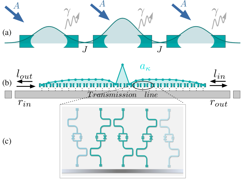
Figure 1: (Color online) (a) Scheme of the driven and dissipative cavity array and (b) input-output measurement using the interaction of the coupled cavity array with an soliton and a transmission line. (c) Sketch of the circuit proposal; curved lines represent superconducting resonators interrupted by a JJ (squares with cross and a capacitor.)

In this work, we will discuss the existence of stationary solitons within the DD-BH. Stationary solitons have an important advantage over exact solutions of conservative equations. Stationary solutions, if stable, are obtained via the dissipative dynamics no matter of the initial state (belonging to the basins of attraction). Therefore their preparation is easier and more robust.

Along this work, we first argue that for the DD-BH model quantum solitons have no anti-continuous limit, i.e, the uncoupled lattice system has a unique stationary solution Drummond and Walls (1980); Le Boité et al. (2013); Boité et al. (2014). This is important, since the single site DD-DNLS for the same parameter regime can have different fixed points in their irreversible dynamics. This is a qualitative difference and should alert to take some care in the utilization of the DD-DNLS for finding solitons. To fix this problem, we include quantum fluctuations up to second order. In doing so, we recover the uniqueness in the stationary single-site solution. Moreover, solitons exists within this (we call it) semiclassical approximation. We discuss their stability and range of existence. We also describe other types of phases appearing when the soliton solution is unstable or absent. We complement our study with a Gutzwiller-Ansatz showing that localization is more persistent within the Gutzwiller in the range where solitons exist within the semiclassical limit. Finally, we discuss a physical realization for the DD-BH based on a circuit-QED architecture Leib et al. (2012). The physical support for our model is complemented with a proposal for a measurement scheme based on an input-output theory, to access the different phases using (already demonstrated) experimental capabilities.

The rest of the paper is organized as follows. The next section II presents the model including dissipation and gain. Besides, we briefly describe the different theoretical approaches used: a second order (in the quantum fluctuations) expansion (SOE) and the Gutzwiller-Ansatz. We finish the section with a possible implementation in circuit QED architectures. In Sect. III we show our numerical results in both approximation schemes and we compare them against the classical DD-DNLS. We present in Sect. IV the input-output formalism for measuring the different phases and conclude with some discussion in. V.

II Model and its (approximate) solutions

The Bose Hubbard (BH) model with driving reads ($\hbar=1$) :

$$H=\sum_{n}\delta\omega a_{n}^{\dagger}a_{n}+\frac{U}{2}a_{n}^{\dagger 2}a_{n}^{2}-J(a_{n+1}^{\dagger}a_{n}+{\rm h.c.})+A(a_{n}^{\dagger}+a_{n})\;.$$ (1)

It marks a minimal model for interacting bosons in a lattice. The model (in the rotating frame of the drive) is characterized via $\delta\omega$ (the detuning of the bare resonator frequency $\omega_{0}$ from the pump frequency $\omega_{d}$, $\delta\omega=|\omega_{0}-\omega_{d}|$), $A$ (the driving amplitude for this coherent external driving), $U$ (the onsite repulsion) and $J$ (the strength of the hopping among sites). Phenomenologically, single-particle-losses can be casted in a Gorini-Kossakowski-Sudarshan-Lindblad master equation Rivas and Huelga (2011)

$$d_{t}\varrho=-i[H,\varrho]+\gamma\sum_{n}a_{n}\varrho a_{n}^{\dagger}-\frac{1}{2}\left\{a_{n}^{\dagger}a_{n},\varrho\right\}$$ (2)

with $\gamma^{-1}$ the time scale for the losses and $\{A,B\}=AB+BA$ the anticonmutator. A pictorial and physical realization based on circuit QED is shown in fig. 1. Without loss and driving, the BH is a cornerstone in many body physics. The generalized BH, Eqs. (1) and (2) mark, then, a paradigmatic model for the study of collective phenomena with driving and dissipation. The dynamical equations for the averages $\langle a_{n}^{\dagger}...a_{m}\rangle\equiv{\rm Tr}(a_{n}^{\dagger}...a_{m}\varrho)$ are given by,

$$i\frac{{\rm d}\langle a_{n}\rangle}{{\rm d}t}=\; (\delta\omega-i\frac{\gamma}{2})\langle a_{n}\rangle+A-J(\langle a_{n+1}\rangle+\langle a_{n-1}\rangle)$$ (3a)

$$+U(2\langle a^{\dagger}_{n}a_{n}\rangle\langle a_{n}\rangle+\langle a_{n}^{2}\rangle\langle a_{n}^{\dagger}\rangle-2\langle a_{n}\rangle^{2}\langle a_{n}^{\dagger}\rangle)$$

$$i\frac{{\rm d}\langle a_{l}^{\dagger}a_{n}\rangle}{{\rm d}t}= -i\gamma\langle a_{l}^{\dagger}a_{n}\rangle+A(\langle a^{\dagger}_{l}\rangle-\langle a_{n}\rangle)+J(\langle a_{l-1}^{\dagger}a_{n}\rangle+\langle a_{l+1}^{\dagger}a_{n}\rangle-\langle a_{l}^{\dagger}a_{n-1}\rangle-\langle a_{l}^{\dagger}a_{n+1}\rangle)$$ (3b)

$$+U(\langle a_{l}^{\dagger}a_{n}^{\dagger}a_{n}a_{n}\rangle-\langle a_{l}^{\dagger}a_{l}^{\dagger}a_{l}a_{n}\rangle)$$

$$i\frac{{\rm d}\langle a_{l}a_{n}\rangle}{{\rm d}t}=\; (2\delta\omega-i\gamma)\langle a_{l}a_{n}\rangle+A(\langle a_{l}\rangle+\langle a_{n}\rangle)-J(\langle a_{l-1}a_{n}\rangle+\langle a_{l+1}a_{n}\rangle+\langle a_{l}a_{n-1}\rangle+\langle a_{l}a_{n+1}\rangle)$$ (3c)

$$+U(\langle a_{l}^{\dagger}a_{l}a_{l}a_{n}\rangle+\langle a_{n}^{\dagger}a_{n}a_{n}a_{l}\rangle+\delta_{n,l}\langle a_{n}a_{n}\rangle)$$

$$\vdots$$

The dots above indicate that, due to the interaction term $Ua_{n}^{\dagger 2}a_{n}^{2}$, an endless hierarchy of equations for the $n$-point correlators $\langle a_{n}^{\dagger}...a_{m}\rangle$ is obtained. Therefore, the set needs to be cut at some order.

II.1 Zeroth order: The DNLS equation

The simplest approximation is the so-called classical limit, consisting in replacing operators by their averages: $\langle a_{n}^{\dagger 2}a_{n}\rangle\to|\varphi_{n}|^{2}\varphi_{n}$, with $\varphi_{n}=\langle a_{n}\rangle$. The approximation can be understood as the zeroth order cumulant expansion in the quantum fluctuations. In doing so, the equation for the first moments (3a) forms already a closed set. The resulting equations are the celebrated DNLS equations, in this case, with driving and dissipation:

$$id_{t}\varphi_{n}=\delta\omega\varphi_{n}+U|\varphi_{n}|^{2}\varphi_{n}-J(\varphi_{n+1}+\varphi_{n-1})+A-\frac{i\gamma}{2}\varphi_{n}\,.$$ (4)

For this set of equations Peschel et al. (2004); Egorov and Lederer (2013), apart from dark soliton and kinks, there also exist bright solitons for a defocusing nonlinearity $U=-1$, on which we will focus along this work. The main question that we tackle is, if the solutions found in the DNLS survive the inclusion of quantum fluctuations.

II.2 Second order expansion

Let us consider now equations (3) up to second order of correlations. In doing so, we rewrite

$$\hat{a}_{n}=\hat{a}_{n}-\langle a_{n}\rangle+\langle a_{n}\rangle=:\delta\hat{a}_{n}+\langle a_{n}\rangle\,.$$ (5)

Neglecting terms with $\mathcal{O}(\delta\hat{a}^{3})\simeq 0$, any $n$-correlator can be written in terms of $2$-point correlators:

$$\langle A_{1}A_{2}A_{3}A_{4}\rangle =\sum_{\begin{subarray}{c}j<k\\ l<m\end{subarray}}\langle A_{j}A_{k}\rangle\langle A_{l}\rangle\langle A_{m}\rangle$$

$$-5\langle A_{1}\rangle\langle A_{2}\rangle\langle A_{3}\rangle\langle A_{4}\rangle\;.$$

Above $j\neq k\neq l\neq m$ and $A_{j}$ can be any annihilation $a_{n}$ (creation $a_{n}^{\dagger}$) operator. Consequently, equations (3a), (3b) and (3c) form a closed set which stands for a second order expansion (SOE). Its numerical solution provides us the results in the subsection III.2. It is worth emphasizing that, instead of the SOE, Gaussian expansions as the Hartree-Fock-Bogoliubov (HFB) or higher order terms might also be considered Tikhonenkov et al. (2007); Witthaut et al. (2011); Quijandría et al. (2014). However, in the parameter regime explored, our SOE approaches better the exact result for the single site case Drummond and Walls (1980).

II.3 Gutzwiller Ansatz

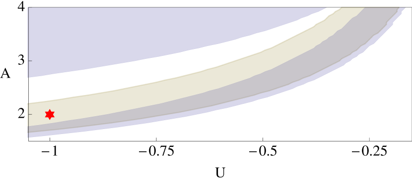
Figure 2: (Color online) Number of single-site solutions vs. $U$ and $A$ for the DNLS and SOE approximation. As explained in the text, forbidden parameter regimes have more than one solution and are shown for DNLS (light gray) and SOE (dark gray). The red star denotes the parameters used along the letter.

To consider higher on-site correlations, we will compare the results of SOE with the time evolution of a density matrix using a Gutzwiller Ansatz Krutitsky et al. (2010); Quijandría et al. (2014) (which assumes a factorized form for the density matrix):

$$\varrho=\prod\limits_{n=1}^{N}\bigotimes\varrho_{n}\,,$$ (7)

with site-dependent density matrices $\rho_{n}$. Using that ${\rm tr}(\varrho_{n})=1$ (${\rm tr}(\partial_{t}\varrho_{n})=0$), we obtain the quantum nonlinear master equation set:

$$\partial_{t}\varrho_{n}=-i\Bigg{[} \delta\omega\,a_{n}^{\dagger}a_{n}+A(a_{n}^{\dagger}+a_{n})+\frac{U}{2}a_{n}^{\dagger 2}a_{n}^{2}$$

$$-J\Bigg{(}\big{(}\langle a_{n+1}^{\dagger}\rangle+\langle a_{n-1}^{\dagger}\rangle)a_{n}+{\rm h.c.}\Bigg{)},\rho_{n}\Bigg{]}$$

$$+\gamma a_{n}\rho_{n}a_{n}^{\dagger}-\frac{1}{2}\left\{a_{n}^{\dagger}a_{n},\rho_{n}\right\}$$ (8)

II.4 Circuit-QED implementation

Though several systems may be modeled by means of a BH model with losses and external driving as in Eqs. (1) and (2), we fix our attention on circuit QED architectures Jin et al. (2013). The latter seem to be an ideal platform to study many body physics Houck et al. (2012). In this subsection we argue that the fundamental blocks for simulating (1) have been already experimentally demonstrated.

The first ingredient is having nonlinear resonators. For that, we think about recent experiments where coplanar waveguide resonators are interrupted by a Josephson Junction (JJ) [Cf. Fig. 1c]. The JJ provides the nonlinearity through the term $E_{J}\cos(2\pi/\Phi_{0}\delta\phi)$ in the effective action. Here $E_{J}$ is the Josephson energy, $\Phi_{0}$ the flux quanta and $\delta\phi$ the jump in the flux at both sides of the junction Zueco et al. (2012); Bourassa et al. (2012). In Ref. Ong et al., 2011, the authors measured nonlinear resonators that can be modeled within the Hamiltonian (after expansion of the cosine):

$$H=\omega_{0}a^{\dagger}a+\frac{U}{2}(a^{\dagger})^{2}a^{2}+\frac{U^{\prime}}{2}(a^{\dagger})^{3}a^{3}+\dots$$ (9)

with $\omega_{0}\cong 6{\rm GHz}$ and $U\cong-700\rm{KHz}$. Therefore, by choosing pumps with driving frequencies detuned from the $\omega_{0}$ on the $\rm KHz-MHz$ regime different $U/\delta\omega$ in (1) can be simulated. Finally, higher order terms can be safely discarded, $U^{\prime}/U\cong 10^{-3}$. An intercavity coupling as in (1):

$$H=J(a^{\dagger}_{n}a_{n+1}+{\rm h.c.})$$ (10)

has been already measured in a wide range of values for $J$, even reaching values of $J/\omega_{0}\cong 0.2$ Haeberlein et al. (2013). Moreover, a tunable coupling $J$ has been measured Baust et al. (2014). Highly reproducibility in the resonator bare frequencies, a necessary ingredient for building many body arrays, has been also achieved Underwood et al. (2012).

Finally, a measurement scheme is mandatory. Here, we rely on the field tomography techniques developed in the circuit QED community Menzel et al. (2010); Bozyigit et al. (2010); Eichler et al. (2011). As explained in section IV, measuring field-field correlators is sufficient for accessing the different phases of (1), including the solitonic solutions. A possible architecture is depicted in figure 1 c). Inspired on Ref. Leib et al., 2012 we envision a one-dimensional array of nonlinear cavities: superconducting resonators interrupted by a JJ. The design is such, that the coupling can be tuned by locally approaching the resonators Haeberlein et al. (2013). The measurement can be accomplished by an auxiliar transmission line that couples the array and where an input field is impinged and the ouput is measured as we will explain in sec. IV. Therefore, the simulation and measurement may be possible within the technological state of the art.

III Results

We summarize here our numerical findings. We first review the classical DNLS limit. Then, we report on our quantum results, both for the SOE and Gutzwiller-Ansatz.

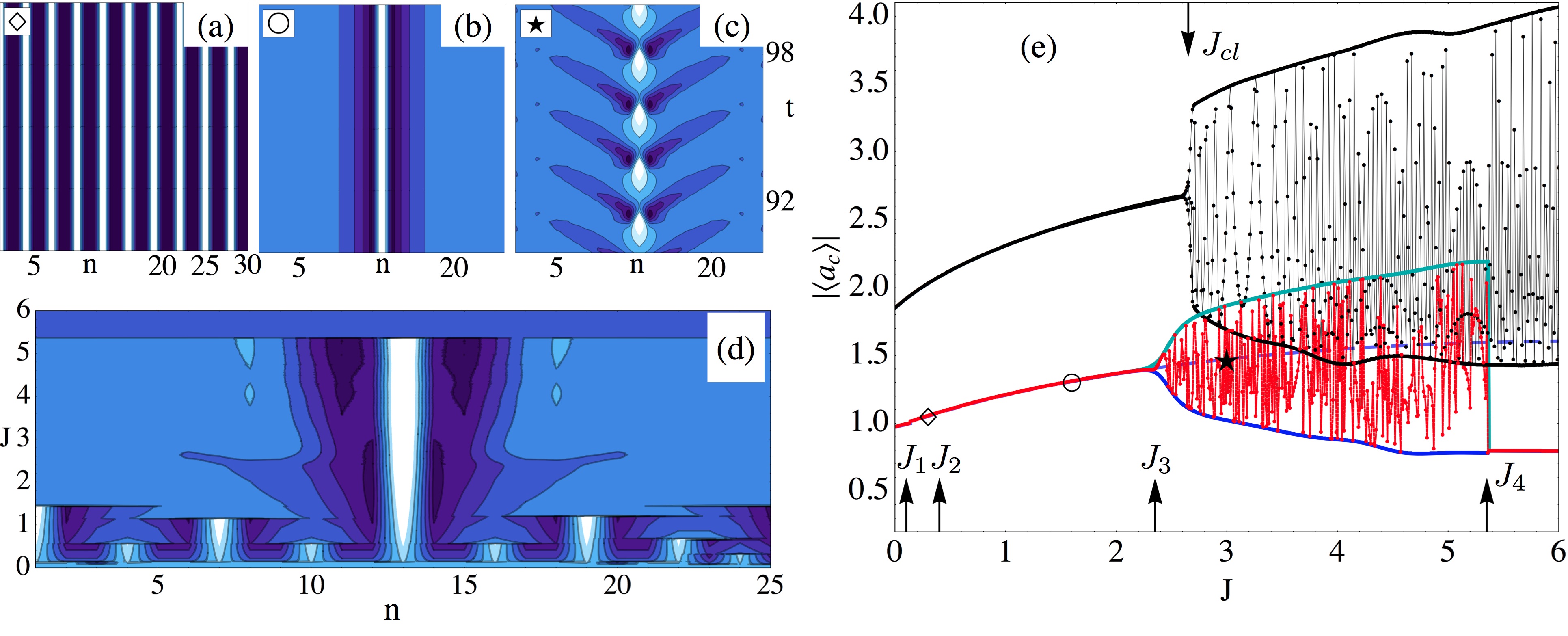
Figure 3: (Color online) Lont-time dynamics of $\langle a_{n}\rangle$ vs. $n$ and $t$ under SOE, showing ripples for $J=0.3$ (a), a stable soliton for $J=1.6$ (b) and the oscillatory localized mode for $J=3$ (c). In (d) SOE steady state of (3) vs. sites $n$ and $J$, in the oscillatory regime $0.5\left(|\langle a_{n}(t_{min})\rangle|+|\langle a_{n}(t_{max})\rangle|\right)$. (e) Amplitude of the center site for DNLS (black), SOE Max(green), SOE Min (blue) and SOE fixed integration time (red) and dashed blue line: unstable localized stationary mode.

III.1 DNLS: solitons with anti-continuous limit

When considering the DNLS one common procedure for finding localized modes is as follows. Imagine that two stable solutions exist for the single site case, say $\varphi$ and $\varphi^{\prime}$. Then, at zero hopping ($J=0$), the solution $\varphi_{m}=\varphi^{\prime}$, $\varphi_{n}=\varphi$ $\forall n\neq m$ is a stable localized solution. This example corresponds to a soliton with a localized amplitude at one site ($m$). This (trivial) soliton can be used as starting point to find solutions by turning on the hopping, $J\neq 0$. In the nonlinear jargon, the zero hopping case is named as anti-continuous limit and MacKay and Aubry (1994); Flach and Gorbach (2008); Kevrekidis (2009) a variety of numerical continuation techniques from zero to non-zero hopping have been used as, for example, the Newton-Raphson method. This procedure is not restricted to conservative settings, but also works very well in the driven dissipative classical models mentioned before. So was used in Peschel et al. (2004); Egorov and Lederer (2013) to characterize the localized modes for the DD-DNLS. The results of this numerical continuation for the DD-DNLS (4) will be compared to SOE in the following.

III.2 SOE: Localization without anti-continous limit

In the quantum regime, the continuation from the zero hopping (anti-continuous limit) can not be used. The reason is, that the single site of (1) and (2) has a unique solution Drummond and Walls (1980). Therefore, if quantum solitons exists they do not have an anti-continuous limit. Without the possibility of finding solitons by continuation, an educated guess is to try the search within the parameter regime where they exist in the classical DNLS limit Peschel et al. (2004); Egorov and Lederer (2013). As anticipated, through this work we use the approximate treatment SOE. Therefore, for consistency, we must check that SOE has a unique solution in the single site case. In figure 2 we delimit this consistency region. Dark-gray areas denote multivalued SOE solutions of (3) and therefore forbidden regions. For comparison we also draw (in light-gray) the forbidden space for the DD-DNLS. The red star marks a point with a unique solution for the SOE but with proven solutions in the DNLS. It seems a good point to start with. The concrete parameters are $U=-1$ $A=\gamma=2$ and -for a better comparison with the DNLS Peschel et al. (2004); Egorov and Lederer (2013)- detuning of $\delta\omega=3+2J$. The only free parameter remaining is the coupling $J$. Those parameters are used along the text.

In general, steady-state solutions can be obtained by simply integrating the dynamics for (3) up to sufficiently long times such that a stationary dynamics is reached. By construction, only stable solutions are found. Besides, there is no necessity of fine-tuned state preparation. Finally, this method provides not only steady-state solutions, but also time-periodic modes. Another possibility, which also finds unstable modes, is using the corresponding algebraic set of equations for $d_{t}\langle\dots\rangle=0$ with e.g. a Newton-Raphson scheme. Unfortunately, this method has no guarantee to converge and could be used successfully only for specific parameters (see the unstable soliton mentioned below). We use the long-time dynamics for all stable modes presented here.

Examples of different solutions assuming periodic boundary conditions are plotted in fig. 3. In figure 3a the dynamics for a stationary ripple mode is depicted. In Fig. 3b) and c) examples for the time evolution of stationary and periodic localized modes are plotted respectively. To visualize the physical mechanism yielding these solutions we choose to plot the mean amplitudes $0.5\left(|\langle a_{n}(t_{min})\rangle|+|\langle a_{n}(t_{max})\rangle|\right)$ vs. sites $n$ and $J$ in Fig. 3d. This averaging is recommendable to better illustrate the localized character of the oscillatory mode, in all other regions of steady-state modes it does not change the picture. The figure shows that, for vanishing and small $J$, the homogeneous mode is the only stable solution. It becomes unstable at $J_{1}\simeq 0.1$, a symmetry-breaking bifurcation not present in the DNLS limit. For small, but finite $J>0.1$ the ripple modes with one site having a higher amplitude than its two neighbors dominate the dynamics. For the spatial periodicity of these modes there is a certain dependency on the number of sites, as can be seen in fig. 3(d) with $n=25$ leading to a defect in the right bottom corner, whereas for $n=30$ in fig. 3 (b) no such defect can be found. As the coupling increases, repeated bifurcations into modes with different periodicity can be observed as the extension of the maxima grows and less peaks can be accommodated within the lattice. Finally, this leads to only one central localized mode in fig. 3(d) at $J_{2}$ appearing dynamically as the steady state. Increasing $J$, the stationary soliton starts to oscillate at $J_{3}$ and finally relaxes to the homogeneous mode for $J_{4}\gtrsim 5.38$. Thus, the SOE does exhibits a train of symmetry breaking bifurcations towards more and more localization, a behavior not found in the DD-DNLS.

We have seen that the classical DNLS is a particular limit of the quantum model in which the quantum fluctuations are neglected. If the quantum corrections were negligible, both the SOE and the DNLS would produce similar results. As shown in Fig. 3(e) this is not the case. There we plot the dependence of the center site amplitude $|\langle a_{c}(t_{evol})\rangle|$ on $J$ after the dynamics settled into a steady-state or periodic state of SOE ((3) (red) within the evolution time $t_{evol}=100$. Please note, that all possible phases are shown in 3(e) and the value of $|\langle a_{c}\rangle|$ does not necessarily indicate that there is a difference to neighbouring sites. The arrows point to the bifurcation points $J_{i}$. When the dynamics is determined by the periodic mode we also show the maximum and minimum of $|\langle a_{c}(t)\rangle|$ in green and blue. The algebraic stationary and unstable localized mode is shown with a blue dashed line. For comparison we show the results of the classical limit (4) in black, also exhibiting a periodic mode, but for higher $J$. The classical amplitude is nearly twice as high as the SOE value, but the main difference is in the classes of solutions found. Whereas the soliton mode is stable in the classical DNLS limit from $J=0$ up to the appearance of the periodic solution at $J_{cl}$, for the SOE limit there is no anti-continuous limit. At $J_{1}$ the ripples appear and persist for $J_{1}<J<J_{2}$. The bifurcation into the periodic solution is located at $J_{3}<J_{cl}$; as well as the high-coupling homogenous mode at $J_{4}$. The symbols in the SOE families denote the examples shown in 3(a)-(c).

III.3 Gutzwiller Ansatz

We complement the SOE with the dynamics within the Gutzwiller Ansatz (7). As initial conditions, we use the homogeneous steady state for the corresponding value of $J$ at all sites but the center, where we assume a coherent state with higher $\langle n_{c}(t=0)\rangle\simeq 8.8$. The Fock-space per lattice site $\rho_{i}$ is truncated to a maximum of $15$ excitations in a lattice of $15$ sites. Within this parameter space, we were able to find a region at $J\simeq 2$, where the initially localized distribution survives much longer. Even though we can compare the SOE and the Gutzwiller Ansatz only qualitatively, this corresponds to the regime of stable soliton modes in the SOE limit. In fig. 4(a) we show the time evolution of $\Delta n_{c,1}(t)=\langle n_{c}(t)\rangle-\langle n_{1}(t)\rangle$ vs. $t$ and $J$, which gives indications about the survival time of localization. Whereas for small $J$ the value of $\Delta n_{c,1}(t)$ decays very fast, the relaxation to the homogeneous state for $J\simeq 2$ is much slower. The values of $\langle n_{i}\rangle$ in the whole array for $J=3.5$ and $J=2$ are plotted in fig. 4 (b) & (c), respectively. Fig. 4(c) shows, that the initial value decays abruptly to $n_{c}\simeq 3$, from that point on the decay becomes very slow. This indicate the existence of a weakly unstable localized mode. For the example shown in fig. 4(b), the initial decay is equally fast, furthermore some oscillations can be observed, which is a reminiscence to the existence of the periodic mode in the SOE limit for these parameter values. Additionally, hints of these oscillations can be seen in $\Delta n_{c,1}$ for $J\simeq 3.5$ . We could not find any indications of an ripples modes, since it presents higher-order inter-site correlations neglected within the Gutzwiller-Ansatz, as we will show in the following section.

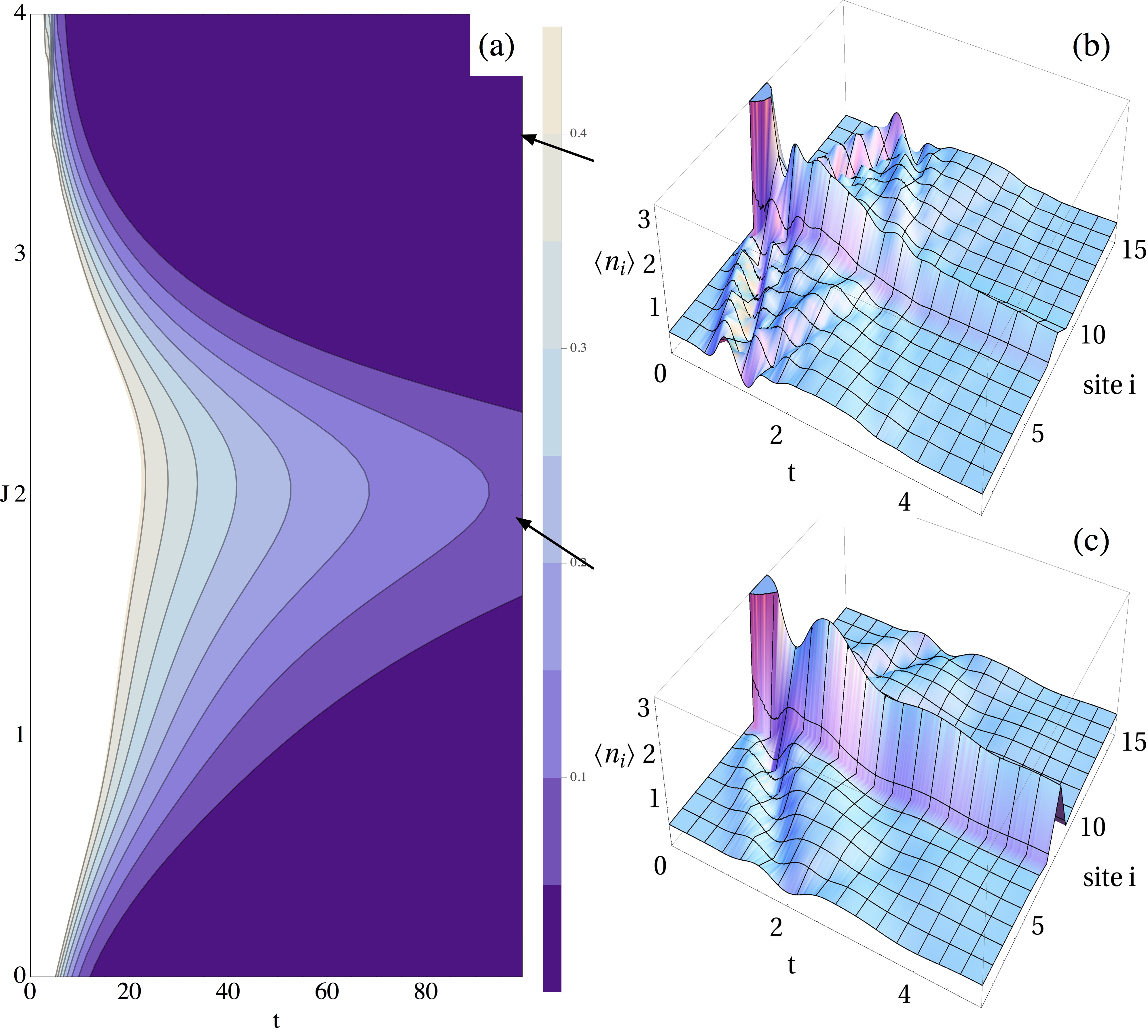
Figure 4: (Color online) Gutzwiller-Ansatz (8): (a) $\langle n_{c}(t)\rangle-\langle n_{1}(t)\rangle$. Left: ${\langle n_{i}(t)\rangle}$ for $J=2$ (b) and $J=3.5$ (c)

IV In-Out mechanism

It still remains the question of how to extract the information stored in our discrete array of cavities. In order to do this, we will follow the input-output formalism Gardiner and Collett (1985). The basic idea here is to make our dissipative system interact with the electromagnetic field (EM), in the form of a transmission line (TL) [Cf. figure 1 b) and c)]. The EM field can be decomposed into two contributions: the input, or the radiation impinging onto the system, and the output, the sum of a reflected plus a radiated component [See Fig.1(b)]. The latter is determined by the system and its interaction with the TL. Therefore, measuring the output (and comparing it with the input) we can infer information on the system dynamics.

We will briefly sketch the main steps to derive the input-output relations. Details on the calculations can be found in Appendix A (see also the Supplementary Material of Ref. Quijandría et al. (2013)). The system we want to acquire information from is an open system described by the Hamiltonian (1) and the master equation (2). Let us denote this open system: the BH model + dissipation and driving as $H_{open}$. The open system $H_{open}$ is coupled to a transmission line as depicted in figure 1 c). The total Hamiltonian, including the TL and the interaction of our system with it, reads $H=H_{\rm open}+H_{\rm TL}+H_{\rm int}$. The TL interacts directly with the cavities and it can be viewed as a one dimensional EM field. In second quantization, the EM field can be described as a collection of harmonic oscillators. As it is depicted in fig. 1 b), we should consider carefully the direction of propagation of excitations in the TL. For this task we will introduce the EM field operators: $l(p)$ ($l^{\dagger}(p)$) which destroys (creates) a photon with momentum $p$ propagating to the left and $r(p)$ ($r^{\dagger}(p)$) which destroys (creates) a photon with momentum $p$ propagating to the right. In terms of these and for a linear dispersion relation ($\omega_{p}=v|p|$), the Hamiltonian of the EM field in the TL reads

$$H_{\rm TL}=v\left(\int_{0}^{\infty}{\rm d}p\,vp\,r^{\dagger}(p)r(p)-\int_{-\infty}^{0}{\rm d}p\,vp\,l^{\dagger}(p)l(p)\right)$$ (11)

with $v$ the speed of light in the TL. Finally, the interaction $H_{\rm int}$ considers the most general type of coupling in a solid-state device. It consists of an inductive part (flux interaction) and a capacitive contribution (charge interaction). The interactions are weak and point-like, happening at the position of every cavity, yielding

$$H_{\rm int} \sim\frac{ig}{\sqrt{2\pi N}}\sum_{k}\left(\int_{+k}\frac{{\rm d}p}{\sqrt{\omega_{p}}}\,N\left(r^{\dagger}(p)a_{k}(t)-{\rm h.c.}\right)\right.$$

$$+\left.\int_{-k}\frac{{\rm d}p}{\sqrt{\omega_{p}}}\,N\left(l^{\dagger}(p)a_{k}(t)-{\rm h.c.}\right)\right)$$ (12)

where we have introduced a plane wave expansion for the cavity operators

$$a_{n}(t)=\frac{1}{\sqrt{N}}\sum_{k}{\rm e}^{ikx_{n}/d}a_{k}(t)$$ (13)

$d$ being the lattice spacing of our cavity array with $N$ sites. We are now able to solve the Heisenberg equations for the left and right operators. The idea is to relate the contributions of all momenta before the interaction (from an initial time $t_{0}\rightarrow-\infty$) and after the interaction (up to a time $t_{1}\rightarrow\infty$). As it is shown in appendix A, for every cavity momentum $k$ we only have significant contributions from those momenta $p$ in a narrow region around the former. For the right operators, we call this momentum interval $+k$ and for the left ones $-k$ [cf. eq. (30)]. Taking this into account, we introduce the (right) input operator

$$r^{+k}_{\rm in}(t)=\frac{1}{\sqrt{2\pi}}\int_{+k}{\rm d}p\,{\rm e}^{-ivp(t-t_{0})}r_{0}(p)$$ (14)

for times $t>t_{0}$ ($r_{0}$ denotes the $r$ operator at $t=t_{0}$) and the (right) output operator

$$r^{+k}_{\rm out}(t)=\frac{1}{\sqrt{2\pi}}\int_{+k}{\rm d}p\,{\rm e}^{-ivp(t-t_{1})}r_{1}(p)$$ (15)

for times $t<t_{1}$ ($r_{1}$ denotes the $r$ operator at $t=t_{1}$). And similarly for the $l$ operators. Thus, the Heisenberg equations lead to the following input-output relations

$$r^{+k}_{\rm out}(t)=r^{+k}_{\rm in}(t)+\frac{1}{d}\sqrt{\frac{\Gamma v}{Nk}}{\rm e}^{-ikvt/d}a_{k}$$ (16)

$$l^{-k}_{\rm out}(t)=l^{-k}_{\rm in}(t)+\frac{1}{d}\sqrt{\frac{\Gamma v}{Nk}}{\rm e}^{+ikvt/d}a_{k}$$ (17)

with $\Gamma$ a constant characterizing the strength of the TL-nonlinear cavity coupling, and $a_{k}$ defined as

$$a_{k}=\frac{1}{\sqrt{2\pi}}\int{\rm d}t^{\prime}\,{\rm e}^{ikvt^{\prime}/d}a_{k}(t^{\prime})$$ (18)

In the presence of the TL the equations of motion for the $a_{k}(t)$ operators differ from those obtained from (2). The TL plays now the role of a second environment for the system described by (1). However, under the same approximations which led to (2) (Markov approximation), we immediately see that the role of the TL is to renormalize the decay rates $\gamma$. Namely, to add a contribution proportional to $g^{2}$ to them. In addition, the input field will renormalize the driving field amplitude (with strength of order $g$).

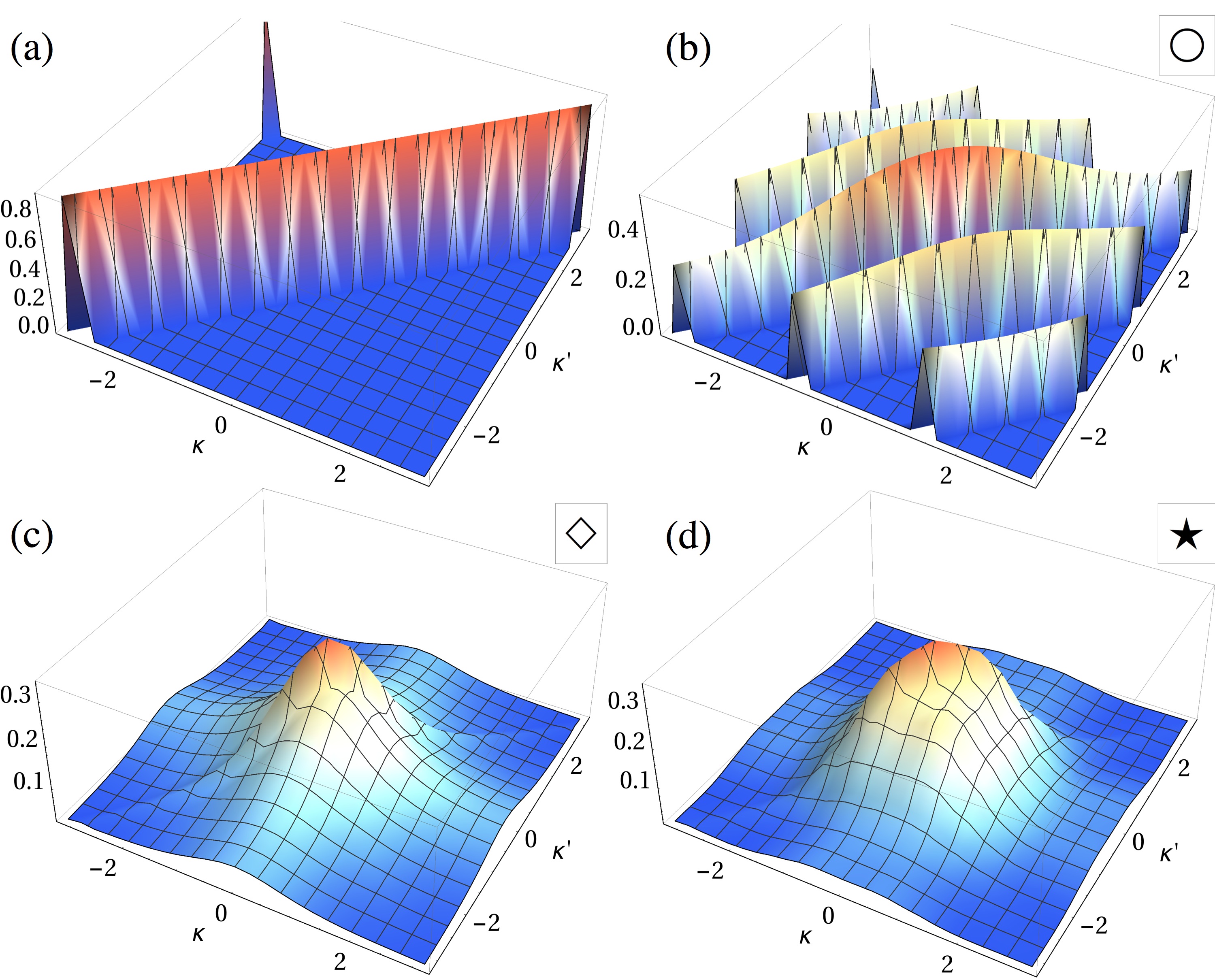
Figure 5: (Color online) Connected correlator $f\left(a_{k},a_{k^{\prime}}^{\dagger}\right)$ (20) for $J=0,(0.3,2,3)$ (a)-(d). For (b)-(d), the symbols correspond to the parameter values and solutions shown in fig. 3(a)-(c).

Within relations (16) and (17) we can map output field-field correlations to cavity modes correlations. For example, using relation (16) $\langle r_{\rm out}^{+k\dagger}(t_{1})r_{\rm out}^{+k}(t_{2})\rangle$ gives us information on the system two-point correlator $\langle a_{k}^{\dagger}a_{k^{\prime}}\rangle$ provided that we only impinge a signal from the left

$$\langle r_{\rm out}^{+k\dagger}(t_{1})r_{\rm out}(t_{2})\rangle=\frac{1}{d^{2}}\left(\frac{\Gamma v}{N\sqrt{kk^{\prime}}}\right){\rm e}^{iv(kt_{1}-k^{\prime}t_{2})/d}\langle a_{k}^{\dagger}a_{k^{\prime}}\rangle$$ (19)

Similar relations hold for other two-point correlations.

Therefore, two time correlations in the output field map to the system two point correlations in momentum space. The first are experimentally accessible, the latter as we will show now provide sufficient information for distinguishing the different phases described throughout this work. We introduce the connected correlator,

$$f(a,b)=\langle ab\rangle-\langle a\rangle\langle b\rangle\,.$$ (20)

It is worth emphasizing that the above is identically zero in the classical limit. In fig. 5 we plot $f\left(a_{k},a_{k^{\prime}}^{\dagger}\right)$ for different stationary SOE solutions. The homogeneous solution ($J=0$) is shown 5 a). The ripples ($J=0.3$) are drawn in 5 b) with the same parameters as in fig. 3 a). Localized solutions, static and oscillatory are given in 5 c) and d) respectively. Their real space counterparts are given in 3 b) and c). The momentum space for each phase are clearly distinguishable from each other and show, that the input-output mechanism presents a perfect measurement scheme to prove the existence and stability of localized modes.

V Discussion

The phases for the Bose-Hubbard model with gain and loss have been investigated within a semi-classical approach. It has been argued that, in the zero hopping case, the unique solution is the homogeneous one. A translational-invariant broken symmetry solution (ripples) appears when the hopping term reaches some critical value. Increasing the hopping, the extension of the ripples grows and their periodicity decreases in a second bifurcation. Eventually, the discrete periodicity disappears and only one maximum remains, the stable localized mode. Passing from static to periodic (in time), this mode finally becomes unstable at higher $J$, transiting to a homogenous solution.

Those successive symmetry-breaking transitions (from homogenous, to discrete periodic, to localized static and periodic modes, and back to homogenous) mark novel phases without counterpart in the Hamiltonian limit (zero dissipation, zero gain) of the Bose-Hubbard where the well known Mott-superfluid transition has been largely described. Apart from the interest in finding novel matter phases in the many body phase diagram, artificial systems with driving and dissipation present also a natural way of observing localization.

Our calculations rely on a semiclassical approximation. We have complemented them with a Gutzwiller Ansatz where the on-site dynamics is expected to be more accurate but inter-site correlations are poorly described. Nevertheless, the regions where solitons exists in the semiclassical regime present long lived localized solutions within the Gutzwiller-Ansatz. Therefore, we expect that the semiclassical phases have some traces in the full, not yet explored, quantum dynamics.

The richness of phases presented here may be a motivation for future works considering the full quantum aspects of the model. In this line, our proposal within circuit QED presents a quantum simulator for going beyond the theory presented here.

Appendix A Input-output theory

Here we derive the input-output relations for the dissipative driven Bose Hubbard model coupled to a transmission line (TL). The total Hamiltonian reads:

$$H=H_{\rm open}+H_{\rm TL}+H_{\rm int}$$ (21)

where $H_{\rm open}$ accounts for the open system: BH model + driving + environment. For simplicity, we will refer to the latter as our system. $H_{\rm TL}$ describes the EM field propagating through the TL. In momentum space it is given by

$$H_{TL}=v\left(\int_{0}^{\infty}{\rm d}p\,vp\,r^{\dagger}(p)r(p)-\int_{-\infty}^{0}{\rm d}p\,vp\,l^{\dagger}(p)l(p)\right)$$ (22)

where we are assuming a linear dispersion relation $\omega_{p}=v|p|$. Our cQED proposal involves impinging a signal into the system and gathering information about it by means of the reflected and transmitted components of the former. For this task, it results helpful to decompose the EM field operators in: $l^{\dagger}(p)$ ($l(p)$) which creates (annihilates) an excitation with momentum $p$ propagating to the left with velocity $v$ (the speed of light in the TL) and similarly, $r^{\dagger}(p)$ ($r(p)$) which creates (annihilates) an excitation with momentum $p$ propagating to the right with velocity $v$. Finally, $H_{\rm int}$ is the interaction Hamiltonian

$$H_{\rm int}=i\sum_{n}\int{\rm d}x\,g_{n}(x)\hat{A}(x)(a_{n}-a_{n}^{\dagger})$$ (23)

Here we are considering a generic coupling between a system operator and the EM potential $\hat{A}(x)$

$$\hat{A}(x) = v\left(\int_{-\infty}^{0}{\rm d}p\sqrt{\frac{1}{2\pi\omega_{p}}}l(p){\rm e}^{ipx}\right.$$ (24)

$$+ \left.\int_{0}^{+\infty}{\rm d}p\sqrt{\frac{1}{2\pi\omega_{p}}}r(p){\rm e}^{ipx}+{\rm h.c.}\right)$$

In Quijandría et al. (2013) following the lumped circuit element description of a TL, we decomposed the interaction into capacitive and inductive contributions. The latter are encoded in the coupling function $g_{n}(x)$. We now introduce a plane wave expansion for the cavity operators $a_{n}$

$$a_{n}(t)=\frac{1}{\sqrt{N}}\sum_{k}{\rm e}^{ikx_{n}/d}a_{k}(t)$$ (25)

where $d$ is the lattice spacing of our cavity array with $N$ sites. Assuming a rotating wave approximation (RWA) regime we can rewrite (23) as

$$H_{\rm int} =\frac{iv}{\sqrt{2\pi N}}\sum_{k,n}$$

$$\times\left[\int_{-\infty}^{0}\frac{{\rm d}p}{\sqrt{\omega_{p}}}\,\int_{-\infty}^{+\infty}{\rm d}x\,g_{n}(x){\rm e}^{-i\left(px-\frac{kx_{n}}{d}\right)}l^{\dagger}(p)a_{k}\right.$$

$$+\left.\int_{0}^{+\infty}\frac{{\rm d}p}{\sqrt{\omega_{p}}}\,\int_{-\infty}^{+\infty}{\rm d}x\,g_{n}(x){\rm e}^{-i\left(px-\frac{kx_{n}}{d}\right)}r^{\dagger}(p)a_{k}\right.$$

$$-\left.{\rm h.c.}\right.\Big{]}$$ (26)

The TL only couples to the system at the position of the cavities, therefore, $g_{n}(x)=g\delta(x-x_{n})$ and we have

$$H_{\rm int} =\frac{ivg}{\sqrt{2\pi N}}\sum_{k}\left(\int_{-\infty}^{0}\frac{{\rm d}p}{\sqrt{\omega_{p}}}\,\sum_{n}\left(l^{\dagger}(p)a_{k}{\rm e}^{-i\left(\frac{\omega_{p}}{v}+\frac{k}{d}\right)x_{n}}\right)\right.$$

$$+\left.\int_{0}^{+\infty}\frac{{\rm d}p}{\sqrt{\omega_{p}}}\,\sum_{n}\left(r^{\dagger}(p)a_{k}{\rm e}^{-i\left(\frac{\omega_{p}}{v}-\frac{k}{d}\right)x_{n}}\right)-{\rm h.c.}\right)$$ (27)

where we have replaced $p$ in the exponentials for $\pm\omega_{p}/v$.

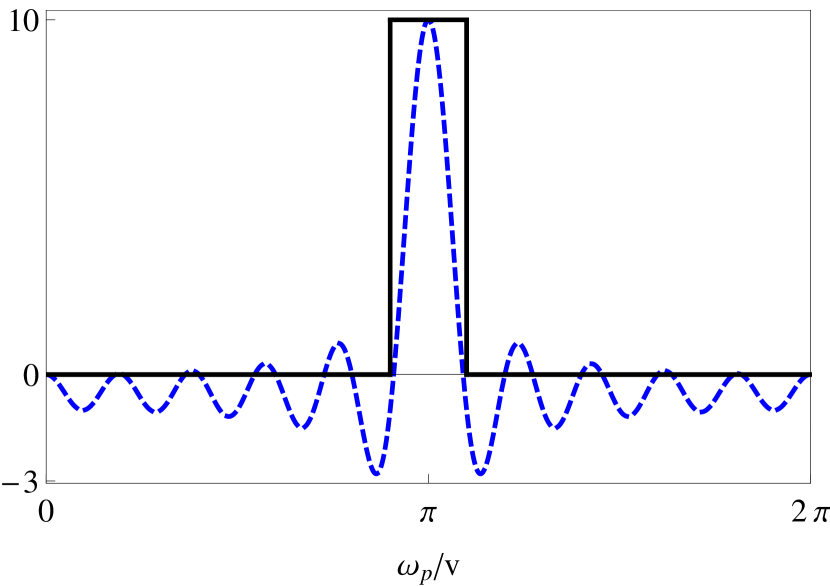
Figure 6: (Color online) Sum (28) (dashed) as a function of $\omega/d$ for $N=10$, and $k/d=\pi$. Rectangle approximation of (28) (full line). This considers that the function is different from zero only in the region between its first two-zeros (symmetric around $k/d$) and that the height is constant and equal to $N$.

We can approximate the sum

$$\sum_{n}{\rm e}^{-i(\omega_{p}/v-k/d)x_{n}}$$ (28)

by a rectangle of height $N$ and width $2\delta=2\pi/N$ centered at $k$ (being zero elsewhere) (see Fig. 6). Similarly, $\sum_{n}{\rm e}^{i(\omega_{p}/v+k/d)x_{n}}$ will be replaced by a rectangle centered in $-k$. Therefore, we can rewrite (A) as

$$H_{\rm int}\sim\frac{ivg}{\sqrt{2\pi N}}\left(\int_{+k}\frac{{\rm d}p}{\sqrt{\omega_{p}}}\,N\left(r^{\dagger}(p)a_{k}-{\rm h.c.}\right)\right.$$

$$\left.+\int_{-k}\frac{{\rm d}p}{\sqrt{\omega_{p}}}\,N\left(l^{\dagger}(p)a_{k}-{\rm h.c.}\right)\right),$$ (29)

where the integration intervals, following our previous approximation, are

$$\pm k\equiv\left[(\pm k-\delta)/d,(\pm k+\delta)/d\right].$$ (30)

We are now able to write the Heisenberg equation of motion for the EM field operators. Following (21), (22) and (A) they are

$$\dot{r}(p)=-ivp\,r(p)+vg\sqrt{\frac{N}{2\pi\omega_{p}}}a_{k}(t)$$ (31)

$$\dot{l}(p)=+ivp\,l(p)+vg\sqrt{\frac{N}{2\pi\omega_{p}}}a_{k}(t)$$ (32)

Here we have included the explicit time dependence of the momentum cavity operators $a_{k}$. Integrating (31) from $t_{0}$ to $t$ ($t_{0}<t$) yields

$$r(p,t) = {\rm e}^{-ivp(t-t_{0})}r_{0}(p)$$ (33)

$$+ vg\sqrt{\frac{N}{2\pi\omega_{p}}}\int_{t_{0}}^{t}dt^{\prime}e^{-ivp(t-t^{\prime})}a_{k}(t^{\prime})$$

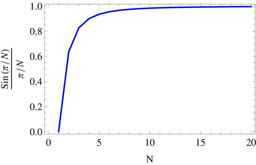
Figure 7: (Color online) $\frac{\sin(y\pi/N)}{y\pi/N}$ as a function of the number $N$ of lattice sites. For $y\sim 1$ the limit $\lim_{z\rightarrow 0}\sin(z)/z=1$ is very well approximated with a few number of sites ($N\sim 10$).

where $r_{0}$ denotes the $r$ operator at time $t=t_{0}$. Notice that the former equations include a continuous momentum $p$ and a discrete one $k$. Recall from our approximation to the sum (28) that for any given $k$ only the momenta $p$ in a very narrow region of width $\delta$ (centered in $k$) contribute to our expressions. We now integrate (33) over this momentum interval ($+k$ for the right operators)

$$\int{\rm d}p\,r(p,t) =\sqrt{2\pi}r^{+k}_{in}(t)$$

$$+g\sqrt{\frac{Nv}{2\pi k}}\int_{t_{0}}^{t}dt^{\prime}\left(\frac{2}{v(t-t^{\prime})}e^{-ikv(t-t^{\prime})/d}\right.$$

$$\times\left.\sin\left(\frac{\delta v(t-t^{\prime})}{d}\right)a_{k}(t^{\prime})\right)$$ (34)

with the input operator $r^{+k}_{\rm in}$ defined as (following Gardiner and Collett (1985))

$$r^{+k}_{\rm in}(t)=\frac{1}{\sqrt{2\pi}}\int_{(k-\delta)/d}^{(k+\delta)/d}{\rm d}p\,{\rm e}^{-ivp(t-t_{0})}r_{0}(p)$$ (35)

We have included the super index $+k$ to stress that this operator sums the momentum contributions in a narrow band around $k$ (positive for the right operators). The input operator takes into account the free evolution of all right-propagating EM field modes before the interaction with the system. Therefore, it acts as a driving field in the equations of motion of the cavity operators. In the continuum limit ($\delta\rightarrow 0$) and for $t_{0}\rightarrow-\infty$, (A) yields

$$\int{\rm d}p\,r(p,t) =\sqrt{2\pi}\left(r^{+k}_{in}(t)+\frac{g}{d}\sqrt{\frac{\pi v}{2Nk}}{\rm e}^{-ikvt/d}a_{k}\right)$$ (36)

as $\delta\rightarrow 0$, we make use of the following limit: $\lim_{z\rightarrow 0}\sin(z)/z=1$ for $z=\delta v(t-t^{\prime})/d$. This holds reasonably well for $N\gtrsim 10$ as it is shown in Fig. 7. In addition, we have introduced

$$a_{k}=\frac{1}{\sqrt{2\pi}}\int_{-\infty}^{+\infty}{\rm d}t^{\prime}{\rm e}^{ikvt^{\prime}/d}a_{k}(t^{\prime})$$ (37)

In a similar way, we can integrate (31) from $t$ to $t_{1}$ ($t<t_{1}$) and define a corresponding output operator.

$$r^{+k}_{\rm out}(t)=\frac{1}{\sqrt{2\pi}}\int_{+k}{\rm d}p\,{\rm e}^{-ivp(t-t_{1})}r_{1}(p)$$ (38)

We will find that the input and output operators are related by

$$r^{+k}_{\rm out}(t)=r^{+k}_{\rm in}(t)+\frac{1}{d}\sqrt{\frac{\Gamma v}{Nk}}{\rm e}^{-ikvt/d}a_{k}$$ (39)

while for the left operators we find

$$l^{-k}_{\rm out}(t)=l^{-k}_{\rm in}(t)+\frac{1}{d}\sqrt{\frac{\Gamma v}{Nk}}{\rm e}^{+ikvt/d}a_{k}$$ (40)

where we have chosen conveniently $g=\sqrt{\Gamma/2\pi}$.

References

- Morsch and Oberthaler (2006) O. Morsch and M. Oberthaler, Rev. Mod. Phys. 78, 179 (2006).
- Blatt and Roos (2012) R. Blatt and C. F. Roos, Nature Phys. 8, 277 (2012).
- Naether et al. (2014) U. Naether, J. J. García-Ripoll, J. J. Mazo, and D. Zueco, Phys. Rev. Lett. 112, 074101 (2014).
- Raftery et al. (2014) J. Raftery, D. Sadri, S. Schmidt, H. Türeci, and a. a. Houck, Phys. Rev. X 4, 031043 (2014).
- Houck et al. (2012) A. A. Houck, H. E. Türeci, and J. Koch, Nature Phys. 8, 292 (2012).
- Kevrekidis (2009) P. Kevrekidis, Springer Tracts in Modern Physics (Springer Berlin Heidelberg, 2009).
- Flach and Gorbach (2008) S. Flach and A. Gorbach, Phys. Rep. 467, 1 (2008).
- Lederer and Stegeman (2008) F. Lederer and G. Stegeman, Phys. Rep. 463, 1 (2008).
- Kartashov et al. (2011) Y. Kartashov, B. Malomed, and L. Torner, Rev. Mod. Phys. 83, 247 (2011).
- Naether et al. (2013) U. Naether, A. J. Martínez, D. Guzmán-Silva, M. I. Molina, and R. A. Vicencio, Phys. Rev. E 87, 062914 (2013), arXiv:/arxiv.org/abs/1212.2936 .
- Krutitsky et al. (2010) K. V. Krutitsky, J. Larson, and M. Lewenstein, Phys. Rev. A 82, 033618 (2010).
- Martin and Ruostekoski (2010) A. D. Martin and J. Ruostekoski, Phys. Rev. Lett. 104, 194102 (2010).
- Witthaut et al. (2011) D. Witthaut, F. Trimborn, H. Hennig, G. Kordas, T. Geisel, and S. Wimberger, Phys. Rev. A 83, 063608 (2011).
- Mishmash et al. (2009) R. Mishmash, I. Danshita, C. Clark, and L. Carr, Phys. Rev. A 80, 053612 (2009).
- Burger et al. (1999) S. Burger, K. Bongs, S. Dettmer, W. Ertmer, and K. Sengstock, Phys. Rev. Lett. 83, 5198 (1999).
- Strecker et al. (2002) K. E. Strecker, G. B. Partridge, A. G. Truscott, and R. G. Hulet, Nature 417, 150 (2002).
- Frantzeskakis (2010) D. J. Frantzeskakis, Jour. Phys. A: Math. 43, 213001 (2010).
- Landa et al. (2010) H. Landa, S. Marcovitch, a. Retzker, M. B. Plenio, and B. Reznik, Phys. Rev. Lett. 104, 043004 (2010).
- Mielenz et al. (2013) M. Mielenz, J. Brox, S. Kahra, G. Leschhorn, M. Albert, T. Schaetz, H. Landa, and B. Reznik, Phys. Rev. Lett. 110, 133004 (2013).
- Peschel et al. (2004) U. Peschel, O. Egorov, and F. Lederer, Opt. Lett. 29, 1909 (2004).
- Prilepsky et al. (2012) J. E. Prilepsky, A. V. Yulin, M. Johansson, and S. a. Derevyanko, Opt. Lett. 37, 4600 (2012).
- Egorov and Lederer (2013) O. A. Egorov and F. Lederer, Opt. Lett. 38, 1010 (2013).
- Johansson et al. (2014) M. Johansson, J. Prilepsky, and S. Derevyanko, Phys. Rev. E , 1 (2014), arXiv:arXiv:1312.7818v2 .
- Jin et al. (2013) J. Jin, D. Rossini, R. Fazio, M. Leib, and M. Hartmann, Phys. Rev. Lett. 110, 163605 (2013).
- Jin et al. (2014) J. Jin, D. Rossini, M. Leib, M. J. Hartmann, and R. Fazio, arXiv preprint , 11 (2014), arXiv:1404.6063 .
- Drummond and Walls (1980) P. Drummond and D. Walls, Jour. Phys. A: Math. 13, 725 (1980).
- Le Boité et al. (2013) A. Le Boité, G. Orso, and C. Ciuti, Phys. Rev. Lett. 110, 233601 (2013), arXiv:arXiv:1212.5444v1 .
- Boité et al. (2014) A. L. Boité, G. Orso, and C. Ciuti, arXiv preprint arXiv:1408.1330 , 1 (2014), arXiv:arXiv:1408.1330v1 .
- Leib et al. (2012) M. Leib, F. Deppe, a. Marx, R. Gross, and M. J. Hartmann, New Jour. Phys. 14, 075024 (2012).
- Rivas and Huelga (2011) A. Rivas and S. F. Huelga, Open Quantum Systems. An Introduction, SpringerBriefs in Physics (Springer Berlin Heidelberg, 2011) p. 100, arXiv:1104.5242v2 .
- Tikhonenkov et al. (2007) I. Tikhonenkov, J. Anglin, and a. Vardi, Phys. Rev. A 75, 013613 (2007).
- Quijandría et al. (2014) F. Quijandría, U. Naether, D. Porras, J. J. García-Ripoll, and D. Zueco, arXiv preprint , 9 (2014), arXiv:1409.0361 .
- Zueco et al. (2012) D. Zueco, J. J. Mazo, E. Solano, and J. J. García-Ripoll, Phys. Rev. B 86 (2012), 10.1103/PhysRevB.86.024503.
- Bourassa et al. (2012) J. Bourassa, F. Beaudoin, J. M. Gambetta, and A. Blais, Phys. Rev. A 86, 013814 (2012), arXiv:arXiv:1204.2237v2 .
- Ong et al. (2011) F. R. Ong, M. Boissonneault, F. Mallet, A. Palacios-Laloy, A. Dewes, a. C. Doherty, A. Blais, P. Bertet, D. Vion, and D. Esteve, Phys. Rev. Lett. 106, 167002 (2011).
- Haeberlein et al. (2013) M. Haeberlein, D. Zueco, P. Assum, T. Weiß l, E. Hoffmann, B. Peropadre, J. García-Ripoll, E. Solano, F. Deppe, A. Marx, and R. Gross, arXiv preprint , 8 (2013), arXiv:1302.0729 .
- Baust et al. (2014) A. Baust, E. Hoffmann, M. Haeberlein, M. J. Schwarz, P. Eder, E. P. Menzel, K. Fedorov, J. Goetz, F. Wulschner, E. Xie, L. Zhong, F. Quijandria, B. Peropadre, D. Zueco, J.-J. Garcia Ripoll, E. Solano, F. Deppe, A. Marx, and R. Gross, arXiv e-prints (2014), arXiv:1405.1969 .
- Underwood et al. (2012) D. Underwood, W. Shanks, J. Koch, and A. Houck, Phys. Rev. A 86 (2012), 10.1103/PhysRevA.86.023837.
- Menzel et al. (2010) E. P. Menzel, F. Deppe, M. Mariantoni, M. A. Araque Caballero, A. Baust, T. Niemczyk, E. Hoffmann, A. Marx, E. Solano, and R. Gross, Phys. Rev. Lett. 105, 100401 (2010).
- Bozyigit et al. (2010) D. Bozyigit, C. Lang, L. Steffen, J. M. Fink, C. Eichler, M. Baur, R. Bianchetti, P. J. Leek, S. Filipp, M. P. da Silva, A. Blais, and A. Wallraff, Nature Phys. 7, 154 (2010).
- Eichler et al. (2011) C. Eichler, D. Bozyigit, C. Lang, L. Steffen, J. Fink, and A. Wallraff, Phys. Rev. Lett. 106, 220503 (2011).
- MacKay and Aubry (1994) R. S. MacKay and S. Aubry, Nonlinearity 7, 1623 (1994).
- Note (1) We check that the condition is fulfilled for the steady-state. For time-periodic solutions we use the corresponding condition for the comparison of two consecutive distributions with maximal center site amplitude.
- Gardiner and Collett (1985) C. Gardiner and M. Collett, Phys. Rev. A 31, 3761 (1985).
- Quijandría et al. (2013) F. Quijandría, D. Porras, J. J. García-Ripoll, and D. Zueco, Phys. Rev. Lett. 111, 73602 (2013).