Hydraulic effects in a radiative atmosphere with ionization

Abstract

Context. In a paper of 1978, Eugene Parker postulated the need for hydraulic downward motion to explain magnetic flux concentrations at the solar surface. A similar process has recently also been seen in simplified (e.g., isothermal) models of flux concentrations from the negative effective magnetic pressure instability.

Aims. We study the effects of partial ionization near the radiative surface on the formation of such magnetic flux concentrations.

Methods. We first obtain one-dimensional (1D) equilibrium solutions using either a Kramers-like opacity or the ${\rm H}^{-}$ opacity. The resulting atmospheres are then used as initial conditions in two-dimensional (2D) models where flows are driven by an imposed gradient force resembling a localized negative pressure in the form of a blob. To isolate the effects of partial ionization and radiation, we ignore turbulence and convection.

Results. In 1D models, due to partial ionization, an unstable stratification forms always near the surface. We show that the extrema in the specific entropy profiles correspond to the extrema in degree of ionization. In the 2D models without partial ionization, strong flux concentrations form just above the height where the blob is placed. Interestingly, in models with partial ionization, such flux concentrations form always at the surface much above the blob. This is due to the corresponding negative gradient in specific entropy. Owing to the absence of turbulence, the downflows reach transonic speeds. With ${\rm H}^{-}$ opacity, flux concentrations are weaker due to the stably stratified deeper parts.

Conclusions. We demonstrate that, together with density stratification, the imposed source of negative pressure drives the formation of flux concentrations. We find that the inclusion of partial ionization affects entropy profiles dramatically causing the strong flux concentrations to form closer to the surface. We speculate that turbulence effects are needed to limit the strength of flux concentrations and homogenize the specific entropy to a more nearly marginal stratification.

1 Introduction

In a series of a papers, Parker (1974, 1976, 1978) introduced the idea of hydraulic flux concentrations at the solar surface. Here the hydraulic device is formed by magnetic flux tubes of varying size and pumping is accomplished by turbulence. In these papers, he envisaged turbulent pumping (analogous to a water jet vacuum pump) as the relevant driver, but other alternatives such as the negative effective magnetic pressure instability (NEMPI), first studied by Kleeorin et al. (1989, 1996), are possible and have also been discussed (Brandenburg et al., 2014).

The flux concentrations of Parker are thought to be just around $100\,{\rm km}$ in diameter. Such tubes can be concentrated further through what is known as convective collapse (Parker, 1978; Spruit, 1979). Although these tubes are only about $100\,{\rm km}$, they might be relevant for sunspots which can be more than a hundred times thicker. Indeed, in the cluster model of sunspots an assembly of many such smaller tubes are thought to constitute a full sunspot. Even today, it is still unclear whether sunspots are monolithic or clustered (see review by Rempel & Schlichenmaier, 2011). Nevertheless, the possibility of downward flows inside sunspots (as seen in Parker’s models of hydraulic magnetic flux concentrations) may be a more universal feature which has also been identified as the driving mechanism in producing magnetic flux concentrations by NEMPI (Brandenburg et al., 2014) and has recently also been seen at the late stages of flux emergence (Rempel & Cheung, 2014).

In most of the work that invokes NEMPI, an isothermal equation of state is used. This allows these effects to be studied in isolation from the downdrafts that occur in convection. However, it is important to assess the effects of thermodynamics and radiation, which might either support or hinder tube formation and amplification.

The goal of the present paper is to investigate how downward flows produce flux concentrations in a partially ionized atmosphere with full radiative transfer. We model the effects of an additional negative pressure by imposing an irrotational forcing function corresponding to a localized gradient force of the form $-\mbox{\boldmath$\nabla$}{}\phi$ on the right-hand side of the momentum equation, where $\phi$ is a localized Gaussian profile function that emulates the effects of negative effective magnetic pressure in a controllable way. By imposing a vertical magnetic field, we force the resulting flow to be preferentially along magnetic field lines. If $\phi$ is chosen to be negative, it corresponds to a negative extra pressure. Horizontal pressure balance then leads to a localized gas pressure and density increase and consequently to a downflow owing to the weight of this density enhancement. The return flow closes in the upper parts of this structure. The resulting flow convergence drives magnetic field lines together and thus forms the magnetic flux concentration envisaged by Parker (1974, 1976, 1978). These flux concentrations are also similar to those seen in studies of NEMPI with a vertical magnetic field (Brandenburg et al., 2013, 2014).

We construct hydrostatic equilibrium solutions using a method similar to that of Barekat & Brandenburg (2014), hereafter BB14. They fixed the temperature at the bottom boundary, which then also fixes the source function for the radiation field. For the opacity we assume here either a generalized Kramers opacity with exponents that result in a nearly adiabatic stratification in the deep fully ionized layers. Alternatively, we use an ${\rm H}^{-}$ opacity that is estimated from the number density of ${\rm H}^{-}$ ions using the Saha equation with a corresponding ionization potential (Kippenhahn & Weigert, 1990). For the purpose of our investigation, it is sufficient to restrict ourselves to the ionization of hydrogen. This approach was also used by Heinemann et al. (2007) in simulations of the fine structure of sunspots.

A general problem in all approaches to time-dependent models of stellar atmospheres is the large gap between acoustic and thermal timescales. Their ratio is of the order of the ratio of the energy flux to $\rho c_{\rm s}^{3}$, where $\rho$ is the density and $c_{\rm s}$ is the sound speed. For the Sun, this ratio is less than $10^{-10}$ in the deeper parts of the convection zone (Brandenburg et al., 2005). This problem has been identified long ago (Chan & Sofia, 1986, 1989) and can be addressed using models that are initially in equilibrium (Nordlund et al., 2009). Another possibility is to consider modified models with a larger flux such that it becomes possible to simulate for a full Kelvin–Helmholtz timescale (Käpylä et al., 2013). This is also the approach taken here and it allows us to construct models whose initial state is very far away from the final one, as is the case with an initially isothermal model.

2 The model

2.1 Governing equations

We adopt the hydromagnetic equations for logarithmic density $\ln\rho$, velocity $\bm{u}$, specific entropy $s$, and magnetic vector potential $A$, in the form

$${{\rm D}{}\ln\rho\over{\rm D}{}t} = -\mbox{\boldmath$\nabla$}{}\cdot\bm{u},$$ (1)

$$\rho{{\rm D}{}\bm{u}\over{\rm D}{}t} = -\mbox{\boldmath$\nabla$}{}(p+\phi)+\rho\mbox{\boldmath$g$}{}+\mbox{\boldmath$J$}{}\times\bm{B}+\mbox{\boldmath$\nabla$}{}\cdot(2\rho\nu\mbox{\boldmath${\sf S}$}{}),$$ (2)

$$\rho T{{\rm D}{}s\over{\rm D}{}t} = -\mbox{\boldmath$\nabla$}{}\cdot\mbox{\boldmath$F$}{}_{\rm rad}+2\rho\nu\mbox{\boldmath${\sf S}$}{}^{2}+\eta\mu_{\rm M}\mbox{\boldmath$J$}{}^{2},$$ (3)

$${\partial\mbox{\boldmath$A$}{}\over\partial t} = \bm{u}\times\bm{B}+\eta\nabla^{2}\mbox{\boldmath$A$}{},$$ (4)

where ${\rm D}{}/{\rm D}{}t=\partial/{\partial t}+\mbox{\boldmath$\nabla$}{}\cdot\bm{u}$, $p$ is the gas pressure, $\mbox{\boldmath$g$}{}=(0,0,-g)$ is the gravitational acceleration, $\nu$ is the viscosity, ${\sf S}_{ij}={\textstyle{1\over 2}}(u_{i,j}+u_{j,i})-{\textstyle{1\over 3}}\delta_{ij}\mbox{\boldmath$\nabla$}{}\cdot\bm{u}$ is the traceless rate-of-strain tensor and $\mbox{\boldmath${\sf S}$}{}^{2}={\sf S}_{ij}{\sf S}_{ji}$ contributes to the (positive definite) viscous heating rate, $\bm{B}=\bm{B}_{0}+\mbox{\boldmath$\nabla$}{}\times\mbox{\boldmath$A$}{}$ is the magnetic field with $\bm{B}_{0}=\hat{\mbox{\boldmath$z$}}{}B_{0}$ representing an imposed vertical magnetic field, $\mbox{\boldmath$J$}{}=\mbox{\boldmath$\nabla$}{}\times\bm{B}/\mu_{\rm M}$ is the current density, $\mu_{\rm M}$ is the magnetic vacuum permeability (not to be confused with the mean molecular weight $\mu$, defined below), $\eta$ is the magnetic diffusivity, and $\mbox{\boldmath$F$}{}_{\rm rad}$ is the radiative flux. For the equation of state, we assume a perfect gas with $p=({\cal R}/\mu)T\rho$, where ${\cal R}=k_{\rm B}/m_{\rm u}$ is the universal gas constant in terms of the Boltzmann constant $k_{\rm B}$ and the atomic mass unit $m_{\rm u}$, $T$ is the temperature, and the dimensionless mean molecular weight is given by

$$\mu(\rho,T)=(1+4x_{\rm He})/(1+y_{\rm H}+x_{\rm He}),$$ (5)

where $y_{\rm H}(\rho,T)$ is the ionization fraction of hydrogen and $x_{\rm He}$ is the fractional number of neutral helium, which is related to the mass fraction of neutral helium $Y$ through $4x_{\rm He}=Y/(1-Y)$. In the following, we use the abbreviation $\mu_{0}=1+4x_{\rm He}=(1-Y)^{-1}=X^{-1}$, where $X$ is the mass fraction of hydrogen (ignoring metals). In relating various thermodynamic quantities to each other, we introduce $\alpha=(\partial\ln\rho/\partial\ln p)_{T}$, which is a known function of $y_{\rm H}$, as well as $\delta=(\partial\ln\rho/\partial\ln T)_{p}$ and the ratio $\gamma=c_{p}/c_{v}$ of specific heats at constant volume and pressure, $c_{v}=(\partial e/\partial T)_{v}$ and $c_{p}=(\partial e/\partial T)_{p}$, respectively, which are known functions of both $y_{\rm H}$ and $T$; see Kippenhahn & Weigert (1990), Stix (2002), and Appendix A. When $y_{\rm H}$ is either $0$ or $1$, we have $\alpha=\delta=1$ and $c_{v}=(3/2)\,{\cal R}/\mu$ with $e=c_{v}T$. In general, however, we have $e=(3/2)\,{\cal R}T/\mu+e_{\rm H}$, where $e_{\rm H}=y_{\rm H}{\cal R}T_{\rm H}/\mu_{0}$ is the specific energy that is used (released) for ionization (recombination) and $T_{\rm H}=\chi_{\rm H}/k_{\rm B}$ is the ionization temperature. Using $\chi_{\rm H}=13.6\,{\rm eV}$ for the ionization energy of hydrogen, we have $T_{\rm H}\approx 1.58\times 10^{5}\,{\rm K}$.

Instead of solving Eq. (3) for $s$, it is convenient to solve directly for $T$ using the relation (Kippenhahn & Weigert, 1990)

$$\rho T{{\rm D}{}s\over{\rm D}{}t}=\rho{{\rm D}{}e\over{\rm D}{}t}+p\mbox{\boldmath$\nabla$}{}\cdot\bm{u}=\rho c_{v}T\left({{\rm D}{}\ln T\over{\rm D}{}t}+{\gamma-1\over\delta}\mbox{\boldmath$\nabla$}{}\cdot\bm{u}\right).\quad$$ (6)

The pressure gradient is computed as

$${1\over\rho}\mbox{\boldmath$\nabla$}{}p={c_{\rm s}^{2}\over\gamma}(\mbox{\boldmath$\nabla$}{}\ln\rho+\delta\mbox{\boldmath$\nabla$}{}\ln T),$$ (7)

where $c_{\rm s}$ is the adiabatic sound speed with $c_{\rm s}^{2}=\gamma p/\rho\alpha$. This approach allows us to find the ionization fraction of hydrogen from the Saha equation as

$${y_{\rm H}^{2}\over 1-y_{\rm H}}={\rho_{\rm e}\over\rho}\left({T_{\rm H}\over T}\right)^{-3/2}\exp\left(-{T_{\rm H}\over T}\right),$$ (8)

where $\rho_{\rm e}=\mu_{0}m_{\rm u}(m_{\rm e}\chi_{\rm H}/2\pi\hbar^{2})^{3/2}$ is the electron density.

To compute $\mbox{\boldmath$\nabla$}{}\cdot\mbox{\boldmath$F$}{}_{\rm rad}$, we adopt the gray approximation, ignore scattering, and assume that the source function $S$ is given by the frequency-integrated Planck function, so $S=(\sigma_{\rm SB}/\pi)T^{4}$, where $\sigma_{\rm SB}$ is the Stefan–Boltzmann constant. The negative divergence of the radiative flux is then given by

$$-\mbox{\boldmath$\nabla$}{}\cdot\mbox{\boldmath$F$}{}_{\rm rad}=\kappa\rho\oint_{4\pi}(I-S)\,{\rm d}{}\Omega,$$ (9)

where $\kappa$ is the opacity per unit mass (assumed independent of frequency) and $I(\bm{x},t,\hat{\mbox{\boldmath$n$}}{})$ is the frequency-integrated specific intensity in the direction $\hat{\mbox{\boldmath$n$}}{}$. We obtain $I$ by solving the radiative transfer equation,

$$\hat{\mbox{\boldmath$n$}}{}\cdot\mbox{\boldmath$\nabla$}{}I=-\kappa\rho\,(I-S),$$ (10)

along a set of rays in different directions $\hat{\mbox{\boldmath$n$}}{}$ using the method of long characteristics. For the opacity, we assume either a Kramers-like opacity $\kappa=\kappa_{0}\rho^{a}T^{b}$ with adjustable coefficients $\kappa_{0}$, $a$, and $b$, or a rescaled ${\rm H}^{-}$ opacity. In the former case, following BB14, it is convenient to express $\kappa$ in the form $\kappa=\tilde{\kappa_{0}}(\rho/\rho_{0})^{a}({T/T_{0}})^{b}$, where $\tilde{\kappa_{0}}$ is a rescaled opacity and is related to $\kappa_{0}$ by $\tilde{\kappa}_{0}=\kappa_{0}\rho_{0}^{a}T_{0}^{b}$. With this choice, the units of $\tilde{\kappa_{0}}$ are independent of $a$ and $b$, and always $\,{\rm Mm}^{-1}\,{\rm cm}^{3}\,{\rm g}^{-1}$ (=$10^{-8}\,{\rm cm}^{2}\,{\rm g}^{-1}$). In the latter case we use for the ${\rm H}^{-}$ opacity the expression (Kippenhahn & Weigert, 1990)

$$\kappa=\kappa_{0}y_{\rm H}(1-y_{\rm H}){\rho\over\rho_{e^{-}}}\!\left({T_{{\rm H}^{-}}\over T}\right)^{3/2}\!\!\exp\left({T_{{\rm H}^{-}}\over T}\right),$$ (11)

where $\kappa_{0}=\sigma_{{\rm H}^{-}}/4\mu_{0}m_{\rm u}$ is a coefficient, $\sigma_{{\rm H}^{-}}=4\times 10^{-17}\,{\rm cm}^{2}$ is the cross section of ${\rm H}^{-}$ (Mihalas, 1978), $x_{Z}=10^{-4}$ is the fraction of metals, $T_{{\rm H}^{-}}=\chi_{{\rm H}^{-}}/k_{\rm B}$ and $\chi_{{\rm H}^{-}}=0.754\,{\rm eV}$ are the ionization temperature and energy of ${\rm H}^{-}$, and $\rho_{e^{-}}=\mu_{0}m_{\rm u}(m_{\rm e}\chi_{{\rm H}^{-}}/2\pi\hbar^{2})^{3/2}$ is the relevant electron density.

An important quantity in a radiative equilibrium model is the radiative conductivity $K=16\sigma_{\rm SB}T^{3}/3\kappa\rho$. According to the results of BB14, $K$ is nearly constant in the optically thick part. This implies that $\rho\propto T^{n}$ with $n=(3-b)/(1+a)$ being effectively a polytropic index of the model provided $n>-1$.

For large values of $T$, the exponential terms in Eqs. (8) and (11) become unity, and only the terms $1-y_{H}\propto\rho/T^{3/2}$ from Eq. (8) and an explicit $\rho/T^{3/2}$ term in Eq. (11) remain. Therefore, $\kappa\propto\rho^{2}T^{-3}$, i.e., $a=2$ and $b=-3$, resulting in a stable stratification with polytropic index $n=(3+3)/(1+2)=2$.

To identify the location of the radiating surface in the model, we compute the optical depth as

$$\tau(x,z,t)=\int_{z}^{L_{z}}(\kappa\rho)(x,z^{\prime},t)\;{\rm d}{}z^{\prime}.$$ (12)

The $\tau=1$ contour corresponds then to the surface from where most of the radiation escapes all the way to infinity. For the forcing function, we assume

$$\phi=\phi_{0}e^{-[x^{2}+(z-z_{0})^{2}]/2R^{2}},$$ (13)

where $\phi_{0}$ is the amplitude with a negative value and $R$ the radius of the blob-like structure.

2.2 Boundary conditions

We consider a two-dimensional (2D) Cartesian slab of size $L_{x}\times L_{z}$ with $-L_{x}/2<x<L_{x}/2$, $0\leq z\leq L_{z}$. We assume the domain to be periodic in the $x$ direction and bounded by stress-free conditions in the $z$ direction, so the velocity obeys

$$\partial u_{x}/\partial z=\partial u_{y}/\partial z=u_{z}=0\quad\mbox{on $\;z=0$, $L_{z}$}.$$ (14)

For the magnetic field we adopt the vertical field condition,

$$\partial A_{x}/\partial z=\partial A_{y}/\partial z=A_{z}=0\quad\mbox{on $\;z=0$, $L_{z}$}.$$ (15)

We assume zero incoming intensity at the top, and compute the incoming intensity at the bottom from a quadratic Taylor expansion of the source function, which implies that the diffusion approximation is obeyed; see Appendix A of Heinemann et al. (2006) for details. To ensure steady conditions, we fix temperature at the bottom,

$$T=T_{0}\quad\mbox{on $z=0$},$$ (16)

while the temperature at the top is allowed to evolve freely. There is no boundary condition on the density, but since no mass is flowing in or out, the volume-averaged density is automatically constant (see Appendix C of BB14). Since most of the mass resides near the bottom, the density there will not change drastically and will be close to its initial value at the bottom.

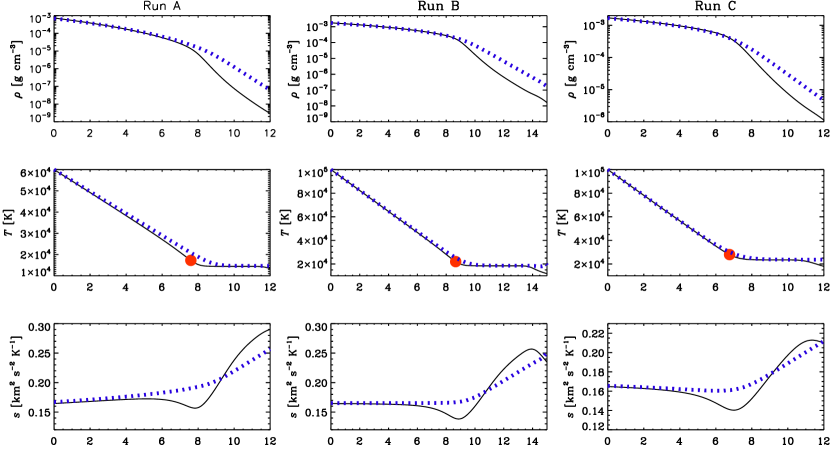
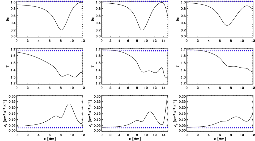
Figure 1: Comparison of $\rho$, $T$, $s$, $y_{\rm H}$, $\gamma$ and $c_{p}$ along each row, top to bottom, from models with (solid) and without (dotted, blue) hydrogen ionization for Runs A, B and C along each column, left to right, and $\tilde{\kappa}_{0}=10^{5}\,{\rm Mm}^{-1}\,{\rm cm}^{3}\,{\rm g}^{-1}$. In the plots of $T(z)$, the closed circles (red) indicate $\tau=1$.

We use for all simulations the Pencil Code, which solves the hydrodynamic differential equations with a high-order finite-difference scheme. The radiation and ionization modules were implemented by Heinemann et al. (2006). All our calculations are carried out either on a one-dimensional (1D) mesh with $576$ points in the $z$ direction or on a 2D mesh with $1152\times 576$ points in the $x$ and $z$ directions.

2.3 Parameters and initial conditions

To avoid very large or very small numbers, we measure length in $\,{\rm Mm}$, speed in $\,{\rm km}\,{\rm s}^{-1}$, density in $\,{\rm g}\,{\rm cm}^{-3}$, and temperature in $\,{\rm K}$. Time is then measured in kiloseconds ($\,{\rm ks}$). We adopt the solar surface value for the gravitational acceleration, which is then $g=274\,{\rm km}^{2}\,{\rm s}^{-2}\,{\rm Mm}^{-1}=2.74\times 10^{4}\,{\rm cm}\,{\rm s}^{-2}$. In most models we use $(a,b)=(1,0)$ and $\tilde{\kappa}_{0}=10^{5}\,{\rm Mm}^{-1}\,{\rm cm}^{3}\,{\rm g}^{-1}$, which yields a top temperature of about $10,000\,{\rm K}$ (BB14). We also present results using the ${\rm H}^{-}$ opacity. In both cases, the opacities are lowered by 5 to 6 orders of magnitude relative to their realistic values to allow thermal relaxation to occur within a few thousand sound travel times. As discussed in BB14, this also leads to a larger flux and therefore a larger effective temperature. For the ${\rm H}^{-}$ opacity, we have applied a scaling factor of $10^{-6}$ in Eq. (11). In all the models we use $\nu=\eta=10^{-3}\,{\rm Mm}\,{\rm km}\,{\rm s}^{-1}$, corresponding to $10^{10}\,{\rm cm}^{2}\,{\rm s}^{-1}$. For the radius of the blob we take $R=1\,{\rm Mm}$ and for the magnetic field we take $B_{0}=1\,{\rm kG}$.

Table 1: Summary of 1D runs leading to equilibrium solutions. For the opacity we either give the values $(a,b)$ for Kramers opacity or we indicate ${\rm H}^{-}$. All runs are carried out on 576 mesh points. $n$ is the polytropic index, $T_{0}$ and $\rho_{0}$ are the initial bottom temperature and density given in $\,{\rm K}$ and $\,{\rm g}\,{\rm cm}^{-3}$, respectively, and $z_{\tau=1}$ is the height where $\tau=1$. Runs A, B and C were carried out with and without ionization.

Run opacity $n$ $T_{0}$ $\rho_{0}$ $z_{\tau=1}$ A $(1,-7/2)$ 3.25 $6\times 10^{4}$ $5\times 10^{-4}$ 7.6 B (1,0) 1.5 $1\times 10^{5}$ $1\times 10^{-3}$ 8.6 C (1,1) 1 $1\times 10^{5}$ $2\times 10^{-3}$ 6.8 D ${\rm H}^{-}$ — $6\times 10^{4}$ $5\times 10^{-4}$ 7.5 E ${\rm H}^{-}$ — $1\times 10^{5}$ $2\times 10^{-3}$ 13.8

Table 2: Summary of 2D models discussed in this paper. For the opacity we either give the values $(a,b)$ for Kramers opacity or we indicate ${\rm H}^{-}$. $\phi_{0}$ and $p(z_{0})$ are given in units of $\,{\rm g}\,{\rm cm}^{-3}\,{\rm km}^{2}\,{\rm s}^{-2}$, while $\max|u_{z}|$ is given in $\,{\rm km}\,{\rm s}^{-1}$.

Run opacity $z_{0}$ $-\phi_{0}$ $p(z_{0})$ $\max|u_{z}|$ F3 (1,0) 3 $3\times 10^{-3}$ 1.00 1.1 K3a (1,0) 3 $3\times 10^{-3}$ 0.94 45 K3b (1,0) 3 $3\times 10^{-4}$ 0.98 40 H3 ${\rm H}^{-}$ 3 $7\times 10^{-4}$ 0.06 22 H10 ${\rm H}^{-}$ 10 $3\times 10^{-2}$ 0.07 15

3 Results

Figure 2: Comparison of models with $\rho_{0}=0.002\,{\rm g}\,{\rm cm}^{-3}$ (solid), $0.005\,{\rm g}\,{\rm cm}^{-3}$ (dashed), and $0.01\,{\rm g}\,{\rm cm}^{-3}$ (dotted lines). Here $(a,b)$ is $(1,0)$, corresponding to $n=1.5$.

First we run 1D simulations with $\phi_{0}=0$ and isothermal initial conditions using Kramers opacity and ${\rm H}^{-}$ opacity. A summary of these runs is listed in Table LABEL:T1summary. We use the resulting equilibrium solutions from the 1D runs as initial conditions for the 2D runs with $\phi_{0}\neq 0$. The summary of 2D runs is listed in Table LABEL:T2summary.

3.1 Kramers opacity

As listed in Table LABEL:T1summary, for Kramers opacity we use three pairs of $(a,b)$, $(1,-3.5)$, $(1,0)$, and $(1,1)$ in Runs A, B, and C, respectively. In the absence of ionization, the resulting equilibrium solutions have an optically thick part that is nearly polytropically stratified, i.e., $\rho\propto T^{n}$, where $n=(3-b)/(1+a)=$3.25, 1.5 and 1, respectively are the polytropic indices (BB14) for Runs A, B and C. In the outer, optically thin part, the temperature in all cases is nearly constant and approximately equal to the effective temperature. For $\gamma=5/3$, a polytropic index of $3/2$ corresponds to an adiabatic stratification. The pressure scale height, $H_{\rm p}={\cal R}T/\mu g$, in the case of $n=1.5$ is about $3\,{\rm Mm}$ in the upper parts of the model and increases to about $7\,{\rm Mm}$ at the bottom. In the 2D runs, for the Kramers opacity, we have used only $(a,b)$ of $(1,0)$, corresponding to $n=1.5$.

In Table LABEL:T1summary we also list the height $z_{\tau=1}$ of the photosphere, where $\tau=1$. For our models with Kramers opacity, the value of $z_{\tau=1}$ is around $8\,{\rm Mm}$, but comparing the models with $T_{0}=10^{5}\,{\rm K}$ and $\rho_{0}=0.002\,{\rm g}\,{\rm cm}^{-3}$ using either Kramers or ${\rm H}^{-}$ opacity (Runs C or E, respectively), we find that $z_{\tau=1}$ doubles from about $7\,{\rm Mm}$ to $14\,{\rm Mm}$, which is the reason we will choose a shallower domain for our 2D experiment.

3.1.1 Vertical equilibrium profiles

In Fig. 1 we compare vertical profiles of various thermodynamic parameters in 1D models with (in solid black) and without (in dotted blue) partial ionization with $\phi_{0}=0$. Both models have in common that the temperature decreases approximately linearly with increasing $z$ and then reaches a constant at a height where $\tau=1$ (in the one with ionization); this height is nearly the same in both cases. By requiring thermostatic equilibrium, Eq. (3) yields $\mbox{\boldmath$\nabla$}{}\cdot\mbox{\boldmath$F$}{}_{\rm rad}=0$, and in the absence of ionization, it is seen that the solutions for the temperature profiles are linearly decreasing for $\tau\gg 1$ and nearly constant for $\tau\ll 1$ (BB14). The inclusion of ionization does not seem to affect the solutions for temperature profiles much. It can be seen that the polytropic density-temperature relation, $\rho\sim T^{n}$, nearly follows in the optically thick part ($\tau>1$) across all atmospheres with different polytropic indices. This is because in the optically thick part, the degree of ionization, $y_{\rm H}$ remains nearly constant.

In the optically thin part, the models with ionization have lower densities compared to the models without ionization, thus increasing the density contrast. The specific entropy in the optically thick part is stratified according to the respective polytropic indices (stable when $n=3.25$, marginal when $n=1.5$, and unstable when $n=1$; cf. BB14).

Interestingly with ionization, all the entropy profiles in Runs A, B, and C behave in a similar fashion near and above the height where $\tau=1$. Near $\tau=1$, there is a narrow layer where the vertical entropy gradient is negative, corresponding to Schwarzschild-unstable stratification and the possibility of convection. (We confirmed this and will comment on it in the discussion.) It can be seen from Fig. 1, that on comparing the specific entropy profiles with the $y_{\rm H}$ profiles, the extrema in the entropy profiles coincide with the ones in the corresponding $y_{\rm H}$ profiles. This correspondence in the extrema between the two quantities, specific entropy and degree of ionization can be shown mathematically. We show in detail in Appendix B that, using the equation of state, the first law of thermodynamics, and the Saha ionization equation, for the case of $\tau\gg 1$,

$${\rm d}{}s={\rm d}{}y_{\rm H}{{\cal R}\over\mu_{0}}\left[{1\over A_{v}}{(n-3/2)\over(n+3/2)}-B_{v}\right],$$ (17)

where $A_{v}$ and $B_{v}$ are coefficients that are defined in Eq. (20) of Appendix A. In the case of $\tau\ll 1$, we have

$${\rm d}{}s={\rm d}{}y_{\rm H}{{\cal R}\over\mu_{0}}\left[{1\over A_{v}}-B_{v}\right].$$ (18)

From Eqs. (17) and (18), we find that the change in specific entropy is directly proportional to the change in degree of ionization and when ${\rm d}{}y_{\rm H}=0$, then ${\rm d}{}s=0$. Thus, the extrema in $s$ directly correspond to extrema in $y_{\rm H}$. The hydrogen ionization fraction $y_{\rm H}$, reaches a minimum of about 0.2 (in Runs A and B) and about 0.4 (Run C) near the surface, but then increases again. This is because of a low density and the exponential decrease in the upper isothermal layer, leading to larger values of $y_{\rm H}$ even when $T$ is small. In the Sun, the surface temperatures are of course smaller still, and therefore $y_{\rm H}\approx 0$ can then be reached. While the specific heats increase outward by a factor of about 5 to 10, their ratio, $\gamma$, decreases below the critical value of 5/3.

In Fig. 2 we compare models with three values of $\rho_{0}$. We recall that $\rho_{0}$ is the bottom value of the density of the initially isothermal model. Since temperature $T_{0}$ is fixed at the bottom, the pressure scale height remains unchanged, but since the stratification evolves to a nearly adiabatic one, the density scale height becomes larger than the pressure scale height, so density drops more slowly and the bottom density becomes smaller by about 2/3; a corresponding expression for this is given by Eq. (C.5) in BB14. Note that models with larger values of $\rho_{0}$ result in lower surface temperatures and lower degrees of ionization near the surface. However, for a given number of mesh points the height of the computational domain has to be reduced for larger values of $\rho_{0}$, because the density drops now much faster to small values. This is just a numerical constraint that can be alleviated by using more mesh points.

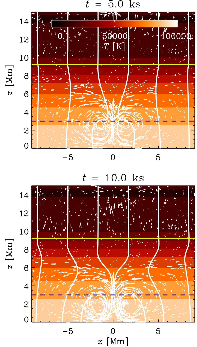
Figure 3: Snapshots of Run F3 (fixed ionization, $y_{\rm H}=1$) showing temperature (color coded), magnetic field lines, and velocity vectors at two times before and after the flux concentration develops. The solid yellow line at $z\approx 9\,{\rm Mm}$ indicates the $\tau=1$ surface while the dashed blue line indicates the height $z_{0}$ where suction operates.

3.1.2 Two-dimensional models

Next, we consider 2D models with $\phi_{0}\neq 0$. The 1D vertical equilibrium solutions form the initial condition here along $z$ for all $x$. We consider first the case $\phi_{0}=-3\times 10^{-3}\,{\rm g}\,{\rm cm}^{-3}\,{\rm km}^{2}\,{\rm s}^{-2}$ using $z_{0}=3\,{\rm Mm}$ for the height of the blob. In Fig. 3 we show the result for Run F3 (fixed ionization, $y_{\rm H}=1$) at $t=5\,{\rm ks}$ and $10\,{\rm ks}$, while in Fig. 4 we show the result for Run K3a with partial ionization effects included at $t=1.6\,{\rm ks}$ and $2\,{\rm ks}$.

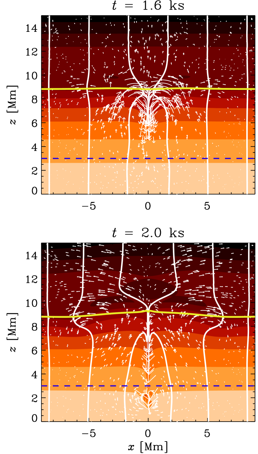
Figure 4: Same as Fig. 3, but for variable partial ionization for Run K3a at two times just before and after the flux concentration develops.

In both the cases (runs F3 and K3a in Figs. 3 and 4), we see the effects of downward suction. We also see how the magnetic field lines are being pushed together at a place above the blob where the return flow tries to replenish the gas in the evacuated upper parts. In the case of partial ionization (Run K3a in Fig. 4), the upper parts have a strongly negative specific entropy gradient leading to an effect that is most pronounced at a height considerably above the height of the blob. Thus, as compared to the case without partial ionization (Run F3), the inclusion of partial ionization (Run K3a) causes the flux concentrations to form at the $\tau=1$ surface. In the Run K3a at the later time, however, when the magnetic structure has collapsed almost entirely, the converging inflow has stopped and there are now indications of an outflow.

Figure 5: Temperature versus optical depth and height at different times through $x=0$ (solid lines and a dotted line for the last time) and $x=L_{x}/2$ (dashed lines) for Run K3a at times $1.6$–$1.9\,{\rm ks}$.

Figure 6: Temperature and vertical magnetic field strength versus $x$ at different times ($1.4$–$2\,{\rm ks}$) through $z=8\,{\rm Mm}$ for Run K3a.

Figure 7: Vertical velocity versus height at different times ($1.6$–$1.9\,{\rm ks}$) for Run K3a.

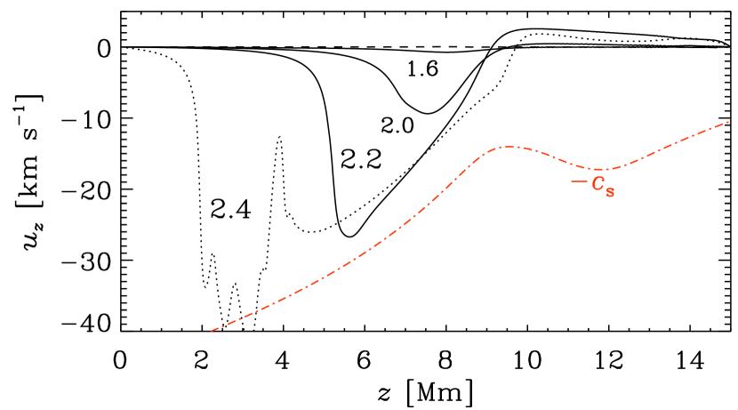
Figure 8: Similar to Fig. 7, but for Run K3b with 10 times weaker suction. The red dash-dotted lines shows the profile of sound speed.

Figure 9: Degree of ionization and ratio or specific heats versus height, from Run K3a.

It is remarkable that at all times, the $\tau=1$ surface is approximately flat, so there is no Wilson depression in our models. To examine whether this is an artifact of the rather small values of opacity in our models, which results in comparatively larger radiative flux and radiative diffusivity, and therefore horizontal temperature equilibration, we ran a similar model, using however only vertical rays in the solution of Eq. (10). However, the results were virtually identical, suggesting that the absence of Wilson depression is not connected with the enhanced luminosity of our models that is used to reduce the Kelvin–Helmholtz timescale.

In Fig. 5 we show for Run K3a vertical temperature profiles though $x=0$ (i.e., through the structure) and $x=L_{x}/2$ (away from it) as functions of $\tau$ and $z$. At $x=0$, we clearly see that for $\tau\gg 1$, the temperature drops progressively below the value at $x=L_{x}/2$. At $z=z_{0}$, the temperature is below $50,000\,{\rm K}$ at $x=0$, while at $x=L_{x}/2$ we have $80,000\,{\rm K}$. Note also that for $\tau<1$, the temperature is slightly enhanced at $x=0$ compared to $x=L_{x}/2$. This is expected, because here the vertical gradient of specific entropy is positive, corresponding to stable stratification, so any downward motion would lead to enhanced entropy and temperature at that position.

In Fig. 6 we show the corresponding temperature and magnetic field profiles through a horizontal cut at $z=8\,{\rm Mm}$, which is just beneath the surface. Note that the temperature is reduced at the location of the structure, but there is also an overall increase in the broader surroundings of the structure, which we associate with the return flow from deeper down. The magnetic field enhancement reaches values of the order of about $50\,{\rm kG}$ (an amplification by a factor of 50) in a narrow spike. These structures are confined by the strong converging return flow.

The downward speed can become comparable with the local sound speed; see Figs. 7 and 8, where we compare two cases with different forcing amplitudes. Nevertheless, in both cases the speeds are similar. This implies that the vertical motion is essentially in free fall. To verify this, we note that the speed of a body freely falling over a distance $\Delta z$ is $v_{\rm ff}=\sqrt{2g\Delta z}$. Using $\Delta z=5\,{\rm Mm}$, we find $v_{\rm ff}\approx 50\,{\rm km}\,{\rm s}^{-1}$, which is comparable with the speeds seen in Figs. 7 and 8. As expected from earlier polytropic convection models with ionization (Rast & Toomre, 1993), the downflow advects less ionized material of lower $\gamma$ and larger $c_{\rm p}$ downward; see Figs. 9 and 10. Then again from time evolution plots of $s$ and $y_{\rm H}$ shown in Figs. 9 and 10, we find a correspondence between the profiles of specific entropy and $y_{\rm H}$, as expected according to Eqs. (17) and (18). Not surprisingly, the suction-induced downflow leads to values of $s$ that, at larger depths inside the structure, agree with the photospheric values higher up. However, temporal changes in $\gamma$ are not as dramatic as the changes with height. Inside the structure, the specific entropy has photospheric values also deeper down, and $s$ is nearly constant (about $0.14\,{\rm km}^{2}\,{\rm s}^{-2}\,{\rm K}^{-1}$) in the range $3\,{\rm Mm}\leq z\leq 9\,{\rm Mm}$ at $t=1.9\,{\rm ks}$.

Figure 10: Specific entropy and specific heat at constant pressure versus height, from Run K3a.

3.2 ${\rm H}^{-}$ opacity

Finally, we compare with models using the ${\rm H}^{-}$ opacity. Again, we use here the implementation of Heinemann et al. (2006, 2007), which was found to yield reasonable agreement with realistic opacities.

3.2.1 One-dimensional equilibrium models

In Fig. 11, we give 1D equilibrium solutions as functions of depth focusing on the top $5\,{\rm Mm}$ (Run D has a height of $9\,{\rm Mm}$, where we have chosen $T_{0}=6\times 10^{4}\,{\rm K}$). The zero on the abscissa coincides with the $\tau=1$ surface and depth $d=z(\tau=1)-z$. We find a stably stratified lower part with an unstable part just beneath the $\tau=1$ surface. The temperature decreases linearly from the bottom, where $K$ is seen to be constant, indicating the regime where the diffusion approximation applies, similar to the other runs with Kramers opacity. However, close to the $\tau=1$ surface there is a short jump (decrease) in the temperature by a factor of $\sim 2$, unlike the runs with Kramers opacity, where the temperature profile simply turns from linearly decreasing to a constant value. The temperature profile eventually settles to a constant for $z>z(\tau=1)$ or $d<0$. This jump in the temperature profile resembles the profile in Fig. 1 and Fig. 14 in Stein & Nordlund (1998), where again the jump is by a factor $\sim 2$ in temperature. It is attributed to the extreme temperature sensitivity of the ${\rm H}^{-}$ opacity.

Figure 11: Profiles of $T$, $s$, $\rho$, $y_{\rm H}$, $\kappa$, and $K$ for Run D, with ${\rm H}^{-}$ opacity. The abscissa gives the depth $d=z(\tau=1)-z$ in $\,{\rm Mm}$.

For comparison, we include Run E, for which we have chosen $T_{0}=10^{5}\,{\rm K}$ and a height of $20\,{\rm Mm}$. The value of $z_{\tau=1}$ is then nearly $14\,{\rm Mm}$. Now, however, there is an extended deeper layer which is stably stratified.

3.2.2 Two-dimensional models

In the 2D model with ${\rm H}^{-}$ opacity, we chose $\phi_{0}=-3\times 10^{-3}\,{\rm g}\,{\rm cm}^{-3}\,{\rm km}^{2}\,{\rm s}^{-2}$ with $z_{0}=3\,{\rm Mm}$ for the height of the blob. In Fig. 12, we see that the flux concentrations form much above the blob location, close to the $\tau=1$ surface. This is again mainly due to the negative gradient in entropy just below $\tau=1$ surface as seen in Fig. 11. Furthermore, there is a very narrow dip in the $\tau=1$ surface in the lower panel of Fig. 12 at $t=1.1\,{\rm ks}$, but is flanked by two peaks, which is due to the return flows.

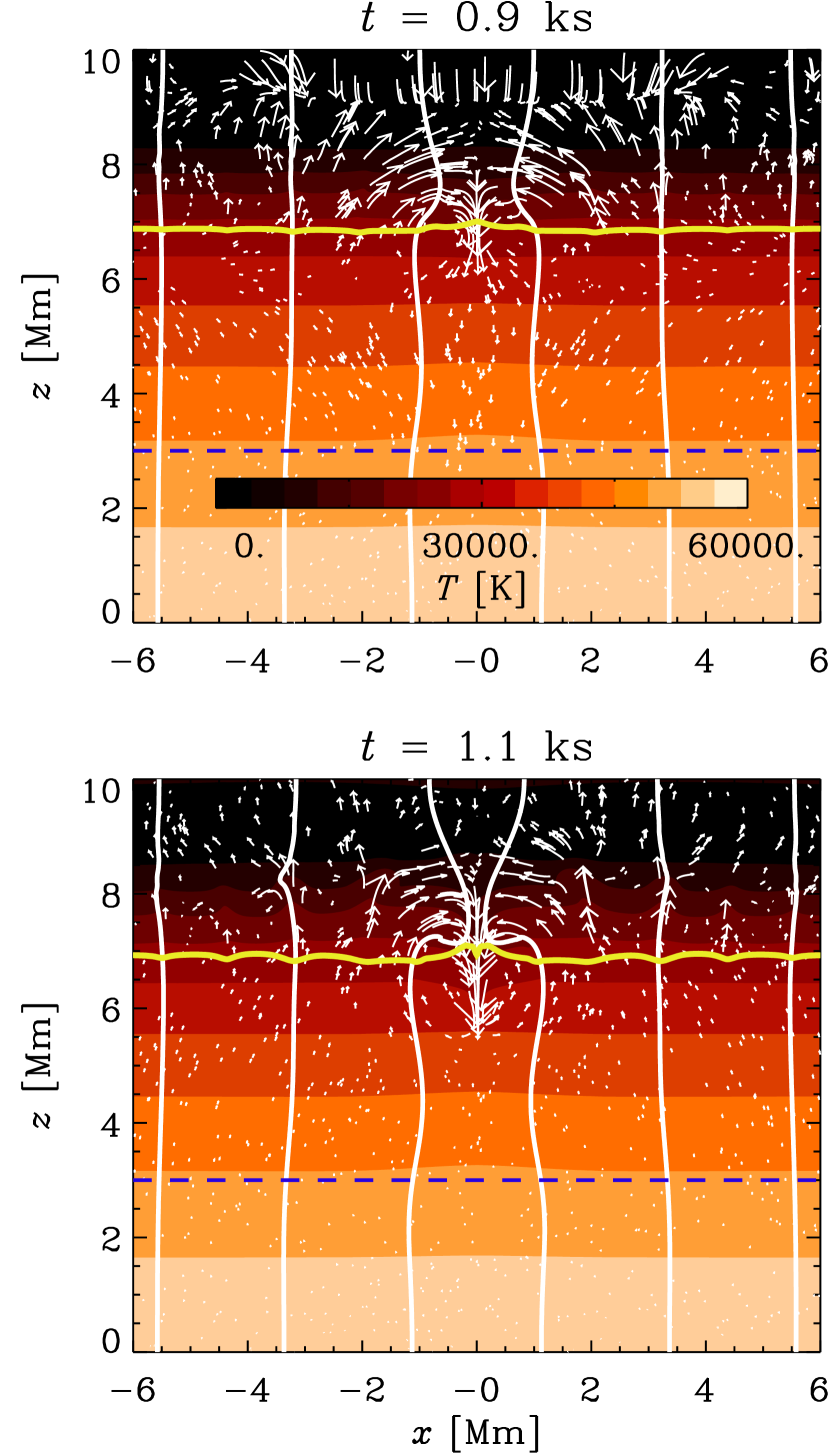
Figure 12: Same as Fig. 4, but for Run H3 using the ${\rm H}^{-}$ opacity with a scaling coefficient of $10^{-6}$.

Owing to the stable stratification of the lower part, the resulting speeds are much lower than those in runs K3a and K3b. As a consequence, the cooling in the temperature profile due to the downflow of low entropy material, shown in Fig. 13, is decreased. Compared to the case of Kramers opacity in Fig. 5, most of the cooling here takes place to much lesser extent in depth. This is further limited because the stratification soon becomes unstable towards larger values of $z$.

Figure 13: Same as Fig. 5, but for Run H3 using the ${\rm H}^{-}$ opacity with a scaling coefficient of $10^{-6}$. Note the increase in temperature at $z\approx 8\,{\rm Mm}$.

Comparing with the deeper model, where $T_{0}=10^{5}\,{\rm K}$ (Run H10, whose equilibrium model was Run E), significant downflows can only be obtained when we place the blob higher up ($z_{0}=10\,{\rm Mm}$) and increase the forcing ($\phi_{0}=-3\times 10^{-2}\,{\rm g}\,{\rm cm}^{-3}\,{\rm km}^{2}\,{\rm s}^{-2}$). This is because of the more extended stably stratified deeper layer. The maximum downflow speed is only $15\,{\rm km}\,{\rm s}^{-1}$.

4 Conclusions

The inclusion of partial ionization along with radiative transfer forms an important step towards bridging the gap between idealized models of magnetic flux concentrations and more realistic ones. In this work, we have studied the effects of partial ionization firstly in 1D hydrostatic models of the atmosphere in thermal equilibrium and then in 2D hydraulic models of flux concentrations. In the radiative transfer module, we have used either Kramers opacity or ${\rm H}^{-}$ opacity.

Comparison of the final 1D equilibrium atmospheres with and without partial ionization shows that, while the solutions do not differ much in the optically thick part, they are significantly different in the range $1<\tau<100$, especially with respect to the specific entropy and density profiles. An interesting feature is the narrow layer with a negative gradient in specific entropy close to the $\tau=1$ surface, which is persistent across different atmospheres with either Kramers opacity (for any polytropic index; shown for $n$= 3.25, 1.5 and 1) or the ${\rm H}^{-}$ opacity. This minimum in the $s$ profile is directly connected to the minimum in $y_{\rm H}$ profile. In fact from Eqs. (17) and (18), it is clear that the extrema in $s$ correspond to the extrema in $y_{\rm H}$. This unstable layer near $\tau=1$ is important since, in the 2D models, it causes the flux concentrations to form right at the surface.

In 1D models with ${\rm H}^{-}$ opacity, the $\tau<1$ part is stably stratified as expected and here also a narrow unstable layer is seen close to surface. Due to the extreme sensitivity of the ${\rm H}^{-}$ opacity to temperature, there is a distinctive jump (by a factor $\sim 2$) in the temperature profile after a prolonged decrease.

In order to study the effect of partial ionization on hydraulic flux concentrations, the model we used employed an artificially imposed source of negative pressure in the momentum equation. This work has demonstrated that such a forcing function can lead to a dramatic downflow that is channeled along vertical magnetic field lines. A corresponding return flow is produced that converges in the upper parts and draws vertical magnetic field lines together, which leads to significant magnetic field amplification. This strong amplification is connected with the high-speed descent of gas. It is much faster than what is expected based on the artificially applied pumping and it is in fact virtually independent of it. Weaker forcing only leads to a delay in what later always tends to develop into nearly free fall. We do not expect such rapid descent speeds to occur in the Sun, because there the gas is turbulent and will behave effectively in a much more viscous and also more irregular fashion, where downdrafts break up and change direction before they can reach significant speeds.

In the case of ${\rm H}^{-}$ opacity, the flux concentrations are weaker because the deeper parts are stably stratified. Here again, the turbulence would have mixed the gas even before triggering downflows, so the background stratification would be more nearly adiabatic to begin with. This can be seen clearly from realistic solar simulations of Stein & Nordlund (1998); see their Fig. 13.

In models without partial ionization, flux concentrations form just above the height where the forcing function is placed, whereas in models including partial ionization, such flux concentrations form at the surface (where $\tau=1$). Here the specific entropy is unstably stratified and tends to drop by a significant amount. Under the influence of downward suction, this could still lead to significant descent speeds with a corresponding return flow as a result of mass conservation. The return flow, instead of closing near the height where the forcing function is placed, closes at the surface, from where the gas had earlier been pulled down.

It is surprising that the temperature reduction inside the downdrafts is rather modest and to some extent compensated for by the supply of hotter material from the converging return flow. Thus, the magnetic structure is in our case largely confined by dynamic rather than gas pressure. Therefore the changes in the thermodynamic properties across the flux tube are only moderate. As a consequence, the $\tau=1$ surface remains nearly flat.

In view of applications to sunspots, it would be important to consider the effects of turbulent convection and its suppression by the magnetic field. Such effects have been used in the models of Kitchatinov & Mazur (2000) that could explain the self-amplification of magnetic flux by a mechanism somewhat reminiscent of the negative effective magnetic pressure instability. In our model, convection would of course develop automatically if we only let the simulation run long enough, because the stratification is already Schwarzschild unstable. The degree to which the resulting convection contributes to the vertical energy transport should increase with increasing opacity, but with the rescaled opacities in our models it will be less than in the Sun.

Our findings also relate to the question of what drives convection in the outer layers of the Sun. Solving just the radiative equilibrium equations for the solar envelope would result in a stable stratification, because the standard Kramers opacity with $a=1$ and $b=-7/2$, corresponding to a stable polytrope with $n=3.25$. Yet, those layers are unstable mainly because of the continuous rain of low entropy material from the top. Clearly, a more detailed investigation of this within the framework of the present model would be needed, but this is well outside the scope of the present paper. Based on the results obtained in the present work, we can say that the effects of partial ionization and resulting stratification are of crucial importance for the production of strong magnetic flux amplifications just near the visible surface.

Appendix A Thermodynamic functions

For completeness, we list here the relevant thermodynamic functions as implemented by Tobias Heinemann into the Pencil Code. We have

$$c_{p}=\left({5\over 2}+A_{p}B_{p}^{2}\right){{\cal R}\over\mu},\quad c_{v}=\left({3\over 2}+A_{v}B_{v}^{2}\right){{\cal R}\over\mu},$$ (19)

as well as $\alpha=A_{p}/A_{v}$ and $\delta=1+A_{p}B_{p}$, where

$$\begin{array}[]{ll}A_{p}={\displaystyle{y_{\rm H}(1-y_{\rm H})\over(2-y_{\rm H})x_{\rm He}+2}},&B_{p}={\displaystyle{5\over 2}+{\chi_{\rm H}\over k_{\rm B}T}},\\ \\ A_{v}={\displaystyle{y_{\rm H}(1-y_{\rm H})\over(2-y_{\rm H})(1+y_{\rm H}+x_{\rm He})}},&B_{v}={\displaystyle{3\over 2}+{\chi_{\rm H}\over k_{\rm B}T}}.\end{array}$$ (20)

Appendix B Effect of partial ionization on entropy profile

On differentiating the equation of state, $p={\cal R}T\rho/\mu$, we have,

$${{\rm d}{}p}=\frac{{\cal R}T}{\mu}{{\rm d}{}\rho}+\frac{\rho{\cal R}}{\mu}{{\rm d}{}T}-\frac{\rho{\cal R}T}{\mu^{2}}{{\rm d}{}\mu}.$$ (21)

Then we express $d\mu$ in terms of $dy_{\rm H}$ using Eq. (5),

$${{\rm d}{}p}=\frac{\rho{\cal R}T}{\mu_{0}}\left[\left({{\rm d}{}\ln\rho}+{{\rm d}{}\ln T}\right)(1+y_{\rm H}+x_{\rm He})+{{\rm d}{}y_{\rm H}}\right].$$ (22)

We substitute Eq. (22) into the equation for first law of thermodynamics, $T{\rm d}{}s={\rm d}{}e+p{\rm d}{}v$, where $v=\rho^{-1}$ is specific volume,

$${{\rm d}{}s}= \frac{1}{T}\left[{{\rm d}{}e}+{{\rm d}{}(pv)}-\frac{1}{\rho}{{\rm d}{}p}\right]$$ (23)

$$= \left(\frac{3{\cal R}}{2\mu_{0}}{{\rm d}{}\ln T}-\frac{{\cal R}}{\mu_{0}}{{\rm d}{}\ln\rho}\right)(1+y_{\rm H}+x_{\rm He})$$ (24)

$$-\frac{{\cal R}}{\mu_{0}}{{\rm d}{}y_{\rm H}}\left[\frac{3}{2}+\frac{\chi_{\rm H}}{k_{B}T}\right],$$

where we have used $e=(3/2)\,{\cal{\cal R}}T/\mu+e_{\rm H}$. Next, differentiate the Saha equation of ionization, $y_{\rm H}^{2}/(1-y_{\rm H})=R$, where

$$R=({\rho_{\rm e}/\rho})\left({T_{\rm H}/T}\right)^{-3/2}\exp\left(-{T_{\rm H}/T}\right),$$ (25)

we have,

$${2y_{\rm H}\over(1-y_{\rm H})}{{\rm d}{}y_{\rm H}}+{y_{\rm H}^{2}\over(1-y_{\rm H})^{2}}{{\rm d}{}y_{\rm H}}={\rm d}{}R$$ (26)

and

$${\rm d}{}R={\rho_{\rm e}/\rho}\left({T_{\rm H}/T}\right)^{-3/2}\exp\left(-{T_{\rm H}/T}\right)\times$$ (27)

$$\left[-{{\rm d}{}\ln\rho}-\frac{3}{2}{{\rm d}{}\ln T}+\frac{\chi_{\rm H}}{k_{B}T}{{\rm d}{}\ln T}\right].$$

After substituting Eq. (27) into Eq. (26), we obtain a relation between ${\rm d}{}y_{\rm H}$, ${\rm d}{}\ln T$ and ${\rm d}{}\ln\rho$,

$${(2-y_{\rm H})\over y_{\rm H}(1-y_{\rm H})}{{\rm d}{}y_{\rm H}}=\left[-{{\rm d}{}\ln\rho}-\left(\frac{3}{2}-\frac{\chi_{\rm H}}{k_{B}T}\right){{\rm d}{}\ln T}\right].$$ (28)

Based on the behaviour of temperature profile we can have two cases, the optically thick $\tau\gg 1$ and the optically thin $\tau\ll 1$. In the case of $\tau\gg 1$, $\rho\propto T^{n}$ and hence, ${\rm d}{}\ln\rho=n\,{\rm d}{}\ln T$. We use this relation in Eq. (28), and have,

$${{\rm d}{}\ln T}=-{1\over(n+1.5)}{(2-y_{\rm H})\over y_{\rm H}(1-y_{\rm H})}{\rm d}{}y_{\rm H}$$ (29)

In the optically thick part, T is large, thus $T_{H}(dT/T^{2})$ is small and can be neglected in Eq. (28). Again we use the relation ${\rm d}{}\ln\rho=n\,{\rm d}{}\ln T$ in Eq. (24) to eliminate ${\rm d}{}\ln\rho$ and finally substitute Eq. (29) into Eq. (24), to obtain,

$${\rm d}{}s={\rm d}{}y_{\rm H}{{\cal R}\over\mu_{0}}\left[{(n-1.5)\over(n+1.5)}{(2-y_{\rm H})(1+y_{\rm H}+x_{\rm He})\over y_{\rm H}(1-y_{\rm H})}\right.$$

$$\left.-{3\over 2}-{\chi_{\rm H}\over k_{B}T}\right].$$ (30)

In the case of $\tau\ll 1$, we use the fact that ${\rm d}{}\ln T=0$ as $T$ is nearly constant here and then obtain,

$${\rm d}{}s={\rm d}{}y_{\rm H}{{\cal R}\over\mu_{0}}\left[{(2-y_{\rm H})(1+y_{\rm H}+x_{\rm He})\over y_{\rm H}(1-y_{\rm H})}-{3\over 2}-{\chi_{\rm H}\over k_{B}T}\right]$$ (31)

Both Eqs. (30) and (31) can be written in the following form using expressions in Eq. (20),

$${\rm d}{}s={\rm d}{}y_{\rm H}{{\cal R}\over\mu_{0}}\left[{1\over A_{v}}{(n-3/2)\over(n+3/2)}-B_{v}\right],$$ (32)

$${\rm d}{}s={\rm d}{}y_{\rm H}{{\cal R}\over\mu_{0}}\left[{1\over A_{v}}-B_{v}\right].$$ (33)

From Eq. (32) and Eq. (33), its clear that the extrema in entropy profile correspond to the extrema in $y_{\rm H}$.

References

- Barekat & Brandenburg (2014) Barekat, A., & Brandenburg, A. 2014, A&A, 571, A68
- Brandenburg et al. (2005) Brandenburg, A., Chan, K. L., Nordlund, Å., & Stein, R. F. 2005, Astron. Nachr., 326, 681
- Brandenburg et al. (2014) Brandenburg, A., Gressel, O., Jabbari, S., Kleeorin, N., & Rogachevskii, I. 2014, A&A, 562, A53
- Brandenburg et al. (2013) Brandenburg, A., Kleeorin, N., & Rogachevskii, I. 2013, ApJ, 776, L23
- Chan & Sofia (1986) Chan, K. L., & Sofia, S. 1986, ApJ, 307, 222
- Chan & Sofia (1989) Chan, K. L., & Sofia, S. 1989, ApJ, 336, 1022
- Heinemann et al. (2006) Heinemann, T., Dobler, W., Nordlund, Å., & Brandenburg, A. 2006, A&A, 448, 731
- Heinemann et al. (2007) Heinemann, T., Nordlund, Å., Scharmer, G. B., & Spruit, H. C. 2007, ApJ, 669, 1390
- Käpylä et al. (2013) Käpylä, P. J., Mantere, M. J., Cole, E., Warnecke, J., & Brandenburg, A. 2013, ApJ, 778, 41
- Kippenhahn & Weigert (1990) Kippenhahn, R., & Weigert, A. 1990, Stellar structure and evolution (Springer: Berlin)
- Kitchatinov & Mazur (2000) Kitchatinov, L. L., & Mazur, M. V. 2000, Solar Phys., 191, 325
- Kleeorin et al. (1989) Kleeorin, N. I., Rogachevskii, I. V., & Ruzmaikin, A. A. 1989, Pis. Astron. Zh., 15, 639
- Kleeorin et al. (1996) Kleeorin, N., Mond, M., & Rogachevskii, I. 1996, A&A, 307, 293
- Mihalas (1978) Mihalas, D. 1978, Stellar Atmospheres (W. H. Freeman: San Francisco)
- Nordlund et al. (2009) Nordlund, Å, Stein, R. F., & Asplund, M. 2009, Liv. Rev. Sol. Phys., 6, 2
- Parker (1974) Parker, E. N. 1974, ApJ, 189, 563
- Parker (1976) Parker, E. N. 1976, ApJ, 210, 816
- Parker (1978) Parker, E. N. 1978, ApJ, 221, 368
- Rast & Toomre (1993) Rast, M. P., & Toomre, J. 1993, ApJ, 419, 224
- Rempel & Cheung (2014) Rempel, M., & Cheung, M. C. M. 2014, ApJ, 785, 90
- Rempel & Schlichenmaier (2011) Rempel, M., & Schlichenmaier, R. 2011, Living Rev. Solar Phys., 8, 3
- Spruit (1979) Spruit, H. C. 1979, Solar Phys., 61, 363
- Stein & Nordlund (1998) Stein, R. F., & Nordlund, Å. 1998, ApJ, 499, 914
- Stix (2002) Stix, M. 2002, The Sun: An introduction (Springer-Verlag, Berlin)