Stochastic hybrid systems in equilibrium: moment closure, finite-time blowup, and exact solutions

Abstract

We present a variety of results analyzing the behavior of a class of stochastic processes — referred to as Stochastic Hybrid Systems (SHSs) — in or near equilibrium, and determine general conditions on when the moments of the process will, or will not, be well-behaved. We also study the potential for finite-time blowups for these processes, and exhibit a set of random recurrence relations that govern the behavior for long times. In addition, we present a connection between these recurrence relations and some classical expressions in number theory.

1 Introduction

1.1 Background and motivation

In this paper, we consider a class of stochastic processes referred to as Stochastic Hybrid Systems (SHSs), and present results about their behavior in or near equilibrium.

One motivation for considering SHSs is if we want to model a system represented by a state that continuously evolves in time (e.g. according to an ODE or an SDE), with the additional complication that the variable, or even the state space itself, can undergo rapid changes. To consider one specific example, consider an engineered system where the state of the system is given by a vector $x(t)\in\mathbb{R}^{d}$ when the system is in “normal” operation, but when the system is in an “impaired” state, only the first $d^{\prime}<d$ variables of the state are able to evolve, and the remainder stay fixed. Moreover, assume that the switching between normal and impaired operation happens randomly, but in a manner that depends on the state $x$.

The study of SHSs has a long history, going back at least to [1]; the main theoretical foundations of the field were laid out in the book [2]. There is a large literature devoted to the understanding the stability analysis of such systems [3, 4, 5] (this stability is typically understood in a moment or almost-sure sense) and more recent work aimed at developing methods to explicitly compute or estimate observables of such systems [6, 7, 8]. Additionally, metastability and large deviations in SHSs were studied in [9] using path-integral methods. SHSs represent a powerful formalism that has been applied to many fields, including: networked control systems [10], power systems [11], system reliability theory [12], and chemical reaction dynamics [13]. A recent review of the state of the art of such systems, that also contains an extensive history, bibliography, and list of applications of SHSs, is the comprehensive review [14].

The state space of an SHS is comprised of a discrete state and a continuous state; the pair formed by these is what we refer to as the combined state of the SHS. One can think of a SHS as a family of stochastic differential equations (SDEs) for the continuous state that are indexed by the discrete state. The discrete state changes stochastically, and we think of this as switching between SDEs. Additionally, each discrete-state transition is associated with a reset map that defines how the pre-transition discrete and continuous states map into the post-transition discrete and continuous states, so that the continuous variable can be “reset” when the discrete state changes. We denote the discrete state space by $\mathcal{{Q}}$, and assume that the continuous state space is $\mathbb{R}^{d}$. Then choose $\left|{\mathcal{{Q}}}\right|$ different SDEs, indexed by $q\in\mathcal{{Q}}$, so that when the discrete state is $q$, $X_{t}$ evolves according to

$$dX_{t}=b_{q}(X_{t})\,dt+\sigma_{q}(X_{t})\,dW_{t}.$$

Then, we assume that there are a family of rate functions $\lambda_{q,q^{\prime}}(x)$ and reset functions $\psi_{q,q^{\prime}}(x)$ such that if the discrete state is $q$, the probability of a jump to state $q^{\prime}$ in the next $\Delta t$ is $\lambda_{q,q^{\prime}}(X_{t})\,\Delta t+o(\Delta t)$, and, if such a jump occurs, the map $\psi_{q,q^{\prime}}$ is applied to the continuous state at the time of jump. [This process can be described more precisely in a “non-asymptotic” formalism, and we do this in Section 2.1.] From this, it follows that there is a continuous-time process, $Q_{t}$, that evolves according to some law, and the full system we are studying is

$$dX_{t}=b_{Q_{t}}(X_{t})\,dt+\sigma_{Q_{t}}(X_{t})\,dW_{t}.$$

It is not hard to show that the process defined in this way is strong Markov [2, §25]. To fully characterize the SHS, we need to compute the expectation of some large class of functions evaluated on its state space. For the purposes of this paper, we want to understand the process in equilibrium, or on the way to equilibrium, i.e., the statistics of the process after it has evolved for a long time. The existence [2, 15] and smoothness [16] of the invariant measure of these processes has been established, and in one sense, the goal of this paper is to explicitly compute as much about this measure as we can, and we approach this by studying the moments of the process, i.e. the expectation of polynomial functions of the process in equilibrium.

Using the infinitesimal generator of the process, following [8, 12], we can write down a set of differential equations for the moments of this process — we refer to this set of equations as the moment flow equations. These equations are a priori infinite-dimensional, and as we show below, in a wide variety of circumstances they are “inherently infinite-dimensional,” by which we mean that: (i) there is no projection of the dynamics onto a finite-dimensional subspace, and (ii) any approximate projection into a finite-dimensional subspace behaves poorly in a sense to be made precise below. This inherent infinite-dimensionality is typically called a moment closure problem in a variety of physical and mathematical contexts, in the sense that one cannot “close” the moment flow equations in a finite way. Examples of moment closure problems and various approaches to handle them span a wide range, including applications in: chemical kinetics [17], dynamic graphs [18, 19, 20], physics [21], population dynamics/epidemiology [22, 23, 24, 25], and nonlinear PDE [26, 27]. Our approach is related to and inspired by the Lyapunov moment stability theory that has been well-developed for diffusions, especially those with small noise, over the past few decades [28, 29, 30, 31].

We mention that a moment closure problem for SHSs was solved nicely in [7, 8] and related works, but in contrast the problem there was to find a moment closure approximation that was valid for a finite time interval. Since we are interested in equilibrium or near-equilibrium statistics of the problem, we want to study the problem on the infinite time interval.

1.2 Overview of the results of this paper

In this paper, we assume that the dynamics on the continuous state are deterministic, i.e., all of the SDEs are assumed to be ODEs, but there is still randomness in how the discrete states switch amongst each other. [These types of systems are also called “randomly switched systems” in the literature [3], but are a subclass of the SHS formalism so it makes sense to have a unifying name.] The fact that the continuous evolution does not have a diffusion term makes the analysis both easier and harder a priori in the sense that the determinism allows for some simplification in certain recurrence relations, but without diffusions, the generator is only hypoelliptic, and thus the existence of, and convergence to, invariant measures for the process is more difficult to establish. We discuss all of these issues below.

In this work, we want to understand the scenario where the two parts of the system (the ODE and the reset) have competing effects. For example, if the ODE and the reset both send all orbits to zero, then their mixture does as well, and, conversely, if they send all orbits to infinity, then the mixture does as well. What is more interesting is the case in which the ODE and the resets have opposite effects, and we consider one such case here: the ODE sends orbits to infinity, but the resets send orbits toward zero.

We give a few prototypical examples of such systems, and discuss the results of this paper that apply to each. In each of these cases, we present a model the continuous variable of which is defined on the positive real line; this can be thought of as the fundamental model of interest, or the radial component of a system in higher dimension (see Section 2.4 for a discussion about dynamics of higher-dimensional systems).

Example 1. Let $\alpha,\beta>0$ and $\gamma\in[0,1]$ and define the ODE, jump rate, and reset as

$$\dot{x}=f(x)=\alpha x,\quad\lambda(x)=\beta x,\quad x\mapsto\gamma x.$$ (1)

The theory presented in Section 3 implies that the SHS in (1) converges to an invariant distribution with all finite moments of all orders, and this fact is independent of the values of $\alpha,\beta,\gamma$ (although of course the moments themselves depend on these parameters).

Example 2. Next, consider the system

$$\dot{x}=f(x)=\alpha x^{2},\quad\lambda(x)=\beta x,\quad x\mapsto\gamma x.$$ (2)

The theory of Section 5 tells us that, depending on the value of $\gamma$, this process can have multiple behaviors: if $\gamma>e^{-\alpha/\beta}$, then all solutions of (2) blow up in finite time, if $1-\alpha/\beta<\gamma<e^{-\alpha/\beta}$, then solutions go to zero with high probability, but enough of them escape to infinite fast enough that the moments of the solution blow up in finite time, but if $\gamma<1-\alpha/\beta$, then the solution converges to zero in every sense. (See Theorem 5.4 for the specific statements.)

Example 3. Finally, consider the system

$$\dot{x}=f(x)=\alpha x^{3},\quad\lambda(x)=\beta x,\quad x\mapsto\gamma x.$$ (3)

Theorem 5.3 tells us that all solutions of this system blowup with probability one, and this fact is independent of the parameters $\alpha,\beta,\gamma$.

Remark 1.1.

The theory in Sections 3 and 5 generalizes the statements in Examples 1 – 3 to arbitrary polynomials. The critical difference between the three cases are the relative degrees, and in some cases the leading-order coefficients, of $f$ and $\lambda$. Additionally, although the two latter cases both exhibit finite-time blowup, they are of a much different character. In the quadratic case, the system blows up in finite time even though there are infinitely many jumps, and as such, exhibit a quality very much like that of an explosive Markov chain. In the cubic case, the blowup is more like that seen in nonlinear ODEs: the system goes off to infinity in finite time and there are only a finite number of jumps.

In Examples 1 – 3, there was a single discrete state and all jumps mapped the state back to itself. We also analyze the moments of the SHS with multiple discrete states in Section 4. We show that the behavior can be characterized similarly to that of one state in many situations, but we also exhibit new types of behavior here. For example, we show that in many cases, the system can exhibit marginal moment stability, by which we mean that in equilibrium, the system can have some moments finite, and others that are infinite; thus the equilibrium distribution has fat tails. In this case, we show numerically that the equilibrium distributions have power law behavior.

We also show that the moment flow equations have a very strange property. These equations are an infinite-dimensional linear system that supports a fixed point that corresponds to the moments of the invariant measure. We show that any finite-dimensional truncation of this system has only unstable fixed points, and, moreover, as the size of truncation grows, the system has larger positive eigenvalues. This motivates the result that the infinite-dimensional system is ill-posed in “the PDE sense” in a manner analogous to a time-reversed heat equation. However, we then show that the minimal amount of convexity given by Jensen’s Inequality is enough to make this system well-posed and well-behaved, and in particular it then becomes faithful to the stochastic process. This seems to be a strange example of a system that is ill-behaved on a linear space becoming well-behaved when restricted to a nonlinear submanifold of that same space.

1.3 Organization of manuscript

The main results and structure of this paper are as follows. In Section 2, we give a formal definition of the SHS that we study, and define the moment flow. Next, we identify a broad class of assumptions for SHSs under which the moment equations are well-defined and accurate on the infinite-time interval, but we also show that there is a surprising subtlety that arises in the consideration of same; these results are contained in Sections 3 and 4. Next, in Section 5, we study the SHS where moment closure fails, and in fact the SHS undergoes finite-time blowups, i.e., the process becomes infinite in expectation, or almost surely, at a finite time. Finally, in Section 6, we write down a few exact recurrence relations for SHSs and show that we can use these, at least in some cases, to compute arbitrarily good approximations.

2 Problem formulation

In this section, we provide the formal definition of the SHS, and define its generator. Then, we use the generator together with Dynkin’s formula to develop a set of differential equations that describe the dynamics of the moments of the SHS. Finally, we provide a description of the SHS using radial components, which allows us to introduce a simplified model of the SHS; analyzing this model is essentially the focus of the remainder of the paper.

2.1 Definition of SHS

Consider a countable set $\mathcal{{Q}}$ of discrete states and a family of phase spaces $P_{q}$, one for each discrete state. We assume that we have defined a family of (random) dynamical systems $D=(D_{q})$, with $D_{q}$ defined on phase space $P_{q}$. The main notion driving SHS is that we want to consider a stochastic process that: (i) in each small timestep $dt$, the system can jump from state $q$ to state $q^{\prime}$ with probability $\lambda_{q^{\prime}}(q,x)\,dt$; and (ii) if it does not jump, it stays in state $q$ and evolves under the dynamics given by $D_{q}$.

As such, we are combining the standard models of a dynamical system on a state space with the notion of a discrete-state Markov process; the system jumps amongst a countable family of states as it would be a Markov chain, and whenever it is in a particular state, it evolves according to the dynamics attached to that state space. Solving the model is complicated by the fact that we allow the jump rates to depend on the state, so that we cannot (for example) determine the jump times and then solve for the continuous flows; they are intimately connected.

For the purposes of this paper, we will assume that the dynamical systems on each phase space are ordinary differential equations (ODEs), but there is no significant obstruction to generalizing the individual flows to SDEs or even general random dynamical systems [5]. We now give the precise definition of a SHS.

Definition 2.1.

A stochastic hybrid system (SHS) is a quintuple $(\mathcal{{Q}},\mathcal{{P}},\Lambda,\Psi,F)$ where

• $\mathcal{{Q}}$ is a countable set of discrete states;

• $\mathcal{{P}}=(P_{q})_{q\in\mathcal{{Q}}}$ are a collection of manifolds, where $P_{q}$ is called the $q$th continuous state space;

• $\Lambda(q,x)=(\lambda_{q^{\prime}}(q,x))_{q^{\prime}\in\mathcal{{Q}}}$ is a collection of rate functions; the domain of $\Lambda$ is $\{(q,x):x\in P_{q},q\in\mathcal{{Q}}\}$ with the property that $\Lambda(q,x)\geq 0$ on its domain. We interpret $\lambda_{q^{\prime}}(q,x)$ as the rate of jumping to discrete state $q^{\prime}$ when the state is currently $(q,x)$.

• $\Psi(q,x)=(\psi_{q^{\prime}}(q,x))_{q^{\prime}\in\mathcal{{Q}}}$ is a collection of reset maps; the domain of $\Psi$ is the same as $\Lambda$, and we assume that $\psi_{q^{\prime}}(q,x)\in P_{q^{\prime}}$. We interpret $\psi_{q^{\prime}}(q,x)$ as the new value of the continuous state immediately after making a $q\mapsto q^{\prime}$ transition.

• $f(q,x)$ is a collection of vector fields, each defined on $P_{q}$, i.e., $f(q,\cdot)\colon P_{q}\to\mathcal{{T}}P_{q}$, where $\mathcal{{T}}P_{q}$ denotes the tangent space to $P_{q}$.

We will denote the flow map generated by $f(q,\cdot)$ by $\varphi^{t}(q,\cdot)$, i.e.,

$$\varphi^{0}(q,x)=x,\quad\varphi^{s}(q,\varphi^{t}(q,x))=\varphi^{s+t}(q,x),\quad\mbox{and }\frac{d}{dt}\varphi^{t}(q,x)=f(q,\varphi^{t}(q,x)).$$

The continuous state space is the disjoint union $\coprod_{q\in\mathcal{{Q}}}P_{q}$ and we call $x\in\coprod_{q\in\mathcal{{Q}}}P_{q}$ a continuous state. When all of the $P_{q}$ are the same, we abuse notation and consider one copy of $P_{q}$ to be the entire continuous state space.

We define the state of the process as the pair $(Q_{t},X_{t})$, and describe its evolution as follows. Let us first assume that $(Q_{t},X_{t})$ is known a.s. for some $t>0$. Let $S^{(q)},q\in\mathcal{{Q}}$ be iid exponential random variables with parameter 1, i.e., $\mathbb{P}(S^{(q)}>z)=e^{-z}$ for all $z\geq 0$, that are also independent of $\{(Q_{s},X_{s}):s\leq t\}$. Define stopping times $T^{(q)},q\in\mathcal{{Q}}$ and $T$ as follows:

$$\int_{t}^{T^{(q)}}\lambda_{q}(Q_{t},\varphi^{s-t}(Q_{t},X_{t}))\,ds=S^{(q)},\quad T=\inf_{q\in\mathcal{{Q}}}T^{(q)}.$$ (4)

Specifically, the $T^{(q)}$ are the times at which each of the transitions to state $q$ would fire, and we take the first one to do so and ignore the others. The time $T$ will be the time of the next jump. We prescribe that the discrete state remains unchanged until the next jump, and the continuous state flows according to the appropriate ODE, i.e.

$$Q_{s}=Q_{t},\quad X_{s}=\varphi^{s-t}(Q_{t},X_{t}),\mbox{ for all }s\in[t,T).$$ (5)

Finally, we apply the appropriate reset map:

$$Q_{T}=\arg\inf_{q\in\mathcal{{Q}}}T_{q},\quad X_{T}=\psi_{Q_{T}}(Q_{t},X_{T-}),$$ (6)

where here and below we define

$$X_{T-}=\lim_{t\nearrow T}X_{t}.$$

Now that we know $(Q_{T},X_{T})$, we can define the process recursively. More specifically, let us define $T_{0}=0$ and assume $(Q_{0},X_{0})$ is known. Then, denote by $T_{1}$ the time returned by the algorithm above, and we have defined $X_{t}$ for $t\in[0,T_{1}]$. For any $n\in\mathbb{N}$, if we know $T_{n}$ and $(Q_{T_{n}},X_{T_{n}})$, then choose $S_{n+1}^{(q)}$ iid exponential, and define $T_{n+1}$ by

$$\int_{t}^{T_{n+1}^{(q)}}\lambda_{q}(Q_{t},\varphi^{s-t}(Q_{t},X_{t}))\,ds=S_{n+1}^{(q)},\quad T_{n+1}=\inf_{q\in\mathcal{{Q}}}T_{n+1}^{(q)}.$$ (7)

Then define $Q_{t},X_{t}$ for $t\in[T_{n},T_{n+1}]$ as in (5, 6).

We also use the convention throughout of minimality: if $T_{\infty}:=\lim_{n\to\infty}T_{n}<\infty$, then we say the process explodes or blows up at time $T_{\infty}$, and set $X_{t}=\infty$ for all $t>T_{\infty}$. Similarly, or if there is a $T^{*}$ with $\lim_{t\nearrow T^{*}}X_{t}=\infty$, then we say the process explodes or blows up at time $T_{*}$, and set $X_{t}=\infty$ for all $t>T_{*}$.

We will also write $(X_{t},Q_{t})=\mathsf{SHS}(\mathcal{{Q}},\mathcal{{P}},\Lambda,\Psi,\varphi)$ to mean that $(X_{t},Q_{t})$ is a realization of the stochastic process constructed using the procedure above.

This definition is complicated and we want to connect the formal definition of the process to an intuitive notion of what it should do.

First, note that it is clear from (5) that between jumps, the continuous state evolves according to the appropriate ODE, and the discrete state remains unchanged. Moreover, from (6) we see that if the system jumps, and it jumps from state $q$ to state $q^{\prime}$, then $Q_{T}$ is updated to the value $q^{\prime}$, and the continuous state is updated by applying the map $\psi_{q^{\prime}}(q,X_{T-})$.

It is also clear from the definition that the process is cadlag (i.e., is right-continuous and has left-limits at every jump, and continuous otherwise). Moreover, the process is stationary, since the ODEs and the rate functions do not depend explicitly on time.

Finally, we intuitively want that, given the current state $(Q_{t},X_{t})$, the probability of a jump occurring in $[t,t+\Delta t)$ should be the sum of all of the current jump rates, i.e., $\sum_{q}\lambda_{q}(Q_{t},X_{t})\Delta t$, and the probability of jumping to state $q^{\prime}$ is equal to the relative proportion of $\lambda_{q^{\prime}}(Q_{t},X_{t})$ to this total rate(qv. Proposition 2.3 below).

Example 2.2.

Before we state and prove Proposition 2.3, let us first consider the special case that many readers will be familiar with, namely, the case where $\lambda_{q^{\prime}}(q,x)$ does not depend on $x$ at all and can be written $\lambda_{q^{\prime}}(q)$. Then the jumps are given by a continuous-time Markov chain (CTMC), and the $\left|{\mathcal{{Q}}}\right|^{2}$ numbers $\lambda_{q^{\prime}}(q)$ are then the transition rates $q\mapsto{q^{\prime}}$. Start at $t=0$, and we obtain

$$\int_{0}^{T^{(q)}}\lambda_{q}(Q_{0})\,ds=S^{(q)},\mbox{ or, }T^{(q)}=S^{(q)}/\lambda_{q}(Q_{0}).$$

It is straightforward to see that the distribution of $T^{(q)}$ is then an exponential random variable of rate $\lambda_{q}(Q_{0})$, i.e.

$$\mathbb{P}(T^{(q)}>t)=e^{-\lambda_{q}(Q_{0})t}.$$

Moreover, if each $T^{(q)}$ is exponential with rate $\lambda_{q}(Q_{0})$, and $T=\inf_{q}T^{(q)}$, then $T$ is exponential of rate $\sum_{q}\lambda_{q}(Q_{0})$ (see, e.g. [32, Theorem 2.3.3]). Finally, $\mathbb{P}(\arg\inf_{q}T_{q}=k)=\lambda_{k}(Q_{0})/\sum_{q}\lambda_{q}(Q_{0})$, and this is independent of $T$. In words, the rate of jumping to state $q$ is the constant rate $\lambda_{q}(Q_{0})$, the total rate of any jump occurring is the sum of the individual rates of each jump occurring, and the probability of any given jump occurring is equal to its proportion to the sum of all the rates.

The only way in which the current framework is more complicated than a standard CTMC is that the transition rates change in time, and they change in such a way as to make them a function of the continuous state.

Proposition 2.3.

We consider the SHS in Definition 2.1 Start the SHS in state $(Q_{0},X_{0})$, and define $T$ as the time of the first jump. Then for $t<T$, the discrete state $Q_{0}$ does not change, and $X_{t}$ evolves according to the ODE, so $X_{t}=\varphi^{t}(Q_{0},X_{0})$. Then

$$\mathbb{P}(T\leq t+\Delta t|T>t) =\Delta t\cdot\sum_{q}\lambda_{q}(Q_{0},X_{t})=\Delta t\cdot\sum_{q}\lambda_{q}(Q_{0},\varphi^{t}(Q_{0},X_{0})),$$

$$\mathbb{P}(Q_{t+\Delta t}=q) =\frac{\lambda_{q}(Q_{0},X_{t})}{\sum_{q^{\prime}}\lambda_{q^{\prime}}(Q_{0},X_{t})}.$$

Proof.

First note that $T>t$ iff $T^{(q)}>t$ for all $q$, and $T\leq t+\Delta t$ iff $T^{(q)}\leq t+\Delta t$ for some $q$. Next, we see that

$$T^{(q)}>t \Leftrightarrow\int_{0}^{t}\lambda_{q}(Q_{0},X_{s})\,ds<S^{(q)},$$

$$T^{(q)}\leq t+\Delta t \Leftrightarrow\int_{0}^{t+\Delta t}\lambda_{q}(Q_{0},X_{s})\,ds\geq S^{(q)},$$

and so

$$\mathbb{P}(T^{(q)}\leq t+\Delta t|T^{(q)}>t) =\mathbb{P}\left(S^{(q)}\leq\int_{0}^{t+\Delta t}\lambda_{q}(Q_{0},X_{s})\,ds\Bigg{|}S^{(q)}>\int_{0}^{t}\lambda_{q}(Q_{0},X_{s})\,ds\right)$$

$$=\mathbb{P}\left(S^{(q)}\leq\int_{0}^{t+\Delta t}\lambda_{q}(Q_{0},X_{s})\,ds-\int_{0}^{t}\lambda_{q}(Q_{0},X_{s})\,ds\right),$$

by the memorylessness property of exponential random variables. But note that for $\Delta t\ll 1$,

$$\int_{0}^{t+\Delta t}\lambda_{q}(Q_{0},X_{s})\,ds-\int_{0}^{t}\lambda_{q}(Q_{0},X_{s})\,ds=\Delta t\cdot\lambda_{q}(Q_{0},X_{t})+o(\Delta t),$$

and

$$\mathbb{P}(S^{(q)}\leq\Delta t\cdot\lambda_{q}(Q_{0},X_{t})+o(\Delta t))=1-\exp(-\Delta t\cdot\lambda_{q}(Q_{0},X_{t})+o(\Delta t))=\Delta t\cdot\lambda_{q}(Q_{0},X_{t})+o(\Delta t).$$

In short, the probability that a jump to $q$ occurs in the next $\Delta t$ is $\Delta t\cdot\lambda_{q}(Q_{0},X_{t})$ when $\Delta t$ is sufficiently small, so the probability that some jump occurs is clearly the sum of these (up to $o(\Delta t)$), and the relative probability of it being $T_{q}$ is the relative proportion of the $q$th rate with respect to the others. ∎

Remark 2.4.

Although the definition is given recursively for simplicity, it is not hard to see that we can choose all of the randomness of this process “up front”, i.e., we can choose streams of iid exponentials $S_{n}^{(q)}$ for $n\in\mathbb{N},q\in\mathcal{{Q}}$ at the beginning, then use these streams to determine the $n$th jump time $T_{n}$ (note that we are discarding all of the $S_{n}^{(q^{\prime})}$ that are not used in this step). This allows us to define a map from any probability space $\Omega$ rich enough to contain the streams $S_{n}^{(q^{\prime})}$ to $\mathcal{{D}}([0,\infty),\mathcal{{Q}}\times\mathcal{{P}})$, the set of cadlag paths defined on $\mathcal{{Q}}\times\mathcal{P}$. This induces a measure on the set of all paths, and, in particular, allows us to measure the probability of any event that can be determined by observing the paths. When we talk about probabilities of events below, we are implicitly assuming that this correspondence has been made. Moreover, this will even allow us to compare paths of two (or more) different SHS that are generated by different functions; as long as we have a correspondence from $\omega\in\Omega$ to the exponential streams $S_{n}^{(q)}(\omega)$, the paths are completely determined by (4). We will use this formalism throughout the remainder of the paper without further comment, and in general drop the dependence on $\omega$.

2.2 Infinitesimal generator

We follow the standard definition of the infinitesimal generator and derive the generator of the process here. Let $h\colon\mathcal{{Q}}\times\mathcal{{P}}\to\mathbb{R}$ be bounded and differentiable, and define the following linear operator $\mathcal{{L}}$:

$$\mathcal{{L}}h(q,x):=\lim_{\epsilon\searrow 0}\frac{\mathbb{E}[h(Q_{t+\epsilon},X_{t+\epsilon})|Q_{t}=q,X_{t}=x]-h(q,x)}{\epsilon}.$$ (8)

From this, we can directly obtain Dynkin’s formula:

$$\frac{d}{dt}\mathbb{E}[h(Q_{t},X_{t})]=\mathbb{E}[\mathcal{{L}}h(Q_{t},X_{t})],$$ (9)

or, said another way, the operator

$$\mathcal{{M}}h(Q_{t},X_{t})=h(Q_{0},X_{0})+\int_{0}^{t}\mathcal{{L}}h(Q_{s},X_{s})\,ds$$ (10)

is a martingale. This allows us to extend the definition of the domain of $\mathcal{{L}}$ through the martingale equation, and it is not hard to show that under weak assumptions on $\Lambda$, $\Psi$, and $f$, the domain of $\mathcal{{L}}$ contains all polynomials [2]. In particular, we can compute directly that

$$\mathcal{{L}}h(q,x)=f(q,x)\cdot\nabla_{x}h(q,x)+\sum_{q^{\prime}\in\mathcal{{Q}}}\lambda_{q^{\prime}}(q,x)\left(h(q^{\prime},\psi_{q^{\prime}}(q,x))-h(q,x)\right).$$ (11)

To give a formal derivation of (11), we compute

$$\mathbb{E}[h(Q_{t+\epsilon},X_{t+\epsilon})-h(Q_{t},X_{t})|Q_{t}=q,X_{t}=x]$$

$$\quad=\mathbb{E}[h(Q_{t+\epsilon},X_{t+\epsilon})-h(Q_{t},X_{t})|Q_{t}=q,X_{t}=x,\mbox{ no jump}]\mathbb{P}(\mbox{no jump})$$

$$\quad\quad+\sum_{q^{\prime}\in\mathcal{{Q}}}\mathbb{E}[h(Q_{t+\epsilon},X_{t+\epsilon})-h(Q_{t},X_{t})|Q_{t}=q,X_{t}=x,\mbox{ jump to $q^{\prime}$}]\mathbb{P}(\mbox{ jump to $q^{\prime}$})$$

$$=(h(q,x+\epsilon f(q,x))-h(q,x))\left(1-O(\epsilon)\right)+\sum_{q^{\prime}\in\mathcal{{Q}}}(h(q^{\prime},\psi_{q^{\prime}}(q,x))-h(q,x))(\epsilon\lambda_{q^{\prime}}(q,x))+O(\epsilon^{2})$$

$$=\epsilon(f(q,x)\cdot\nabla_{x}h(q,x)+\sum_{q^{\prime}\in\mathcal{{Q}}}\lambda_{q^{\prime}}(q,x)\left(h(q^{\prime},\psi_{q^{\prime}}(q,x))-h(q,x)\right))+O(\epsilon^{2}),$$

and from this and the definition of $\mathcal{{L}}$ we have established (11) formally. We have not been careful to specify the domain of $\mathcal{{L}}$, but it is clear from this argument that this derivation is valid for all $h\in C^{1}\cap L^{\infty}$. As is shown in [2], we can then extend the domain of the generator using (10) to encompass all polynomials and indicator functions. Strictly speaking, this means that the new generator is an extension of the previous one, and we will use this without further comment in the sequel.

2.3 Moment equations

A quick perusal of (11) makes it clear that if we assume that $f(q,\cdot)$, $\lambda_{q^{\prime}}(q,\cdot)$, $\psi_{q^{\prime}}(q,\cdot)$ are polynomials in $x$, then the right-hand side sends polynomials to polynomials. More precisely, if $h(q,x)$ is any function that is polynomial in $x$, then $\mathcal{{L}}h(q,x)$ is also polynomial in $x$. In particular, we denote $h^{(m)}_{q^{\prime}}(q,x)=x^{m}\delta_{q,q^{\prime}}$, and we see that $\mathcal{{L}}h^{(m)}_{q}$ is a polynomial in $x$, so that Dynkin’s formula becomes an (infinite-dimensional) linear ODE on the set $\{h^{(m)}_{q}\}_{m\in\mathbb{N}^{d},q\in\mathcal{{Q}}}$. However, the first challenge that we obtain is clear: if the degree of any $f(q,\cdot)$ is greater than one, or the degree of any of the $\lambda_{q^{\prime}}(q,\cdot)$ or $\psi_{q^{\prime}}(q,\cdot)$ are positive, then we see that the degrees of the terms on the right-hand side of the equation are higher than those on the left, and we are thus led to the problem of moment closure. On the other hand, we still have a linear system, even if it is infinite-dimensional. Thus, we might hope to make sense of this flow by writing down a semigroup on a reasonable function space. In fact, we show in Section 3.2 that this is in general not possible.

2.4 Radial components

Consider the case where $\mathcal{P}_{q}=\mathbb{R}^{d}$ for all $q$, and we can abuse notation slightly and identify $\mathbb{R}^{d}$ as the continuous state space. Consider the ODE

$$\frac{d}{dt}X_{t}=f(Q_{t},X_{t})$$

for $X_{t}\in\mathbb{R}^{d}$. Write $X_{t}=R_{t}U_{t}$, for $R_{t}\in[0,\infty)$ and $U_{t}\in S^{d-1}$. Since $R_{t}^{2}=\sum_{k=1}^{d}X_{t,k}^{2}$, we see that

$$2R_{t}\frac{d}{dt}R_{t}=\sum_{k=1}^{d}2X_{t,k}\frac{d}{dt}X_{t,k}=\sum_{k=1}^{d}2X_{t,k}f_{k}(Q_{t},X_{t}),$$

or

$$\frac{d}{dt}R_{t}=\frac{\sum_{k=1}^{d}2X_{t,k}f_{k}(Q_{t},X_{t})}{\sum_{k=1}^{d}X_{t,k}^{2}}=:\rho(Q_{t},X_{t}).$$

In general, this depends on both $R_{t}$ and $U_{t}$ through $X_{t}$, and we cannot project the dynamics onto $R_{t}$. However, if we assume that $\rho(q,x)$, $\lambda_{q^{\prime}}(q,x)$, and $\psi_{q^{\prime}}(q,x)$ are independent of the angular component of $x$, then we can consider a purely radial model for the dynamics and consider an SHS whose continuous state space is the positive real axis.

More generally, consider the following: consider the system $\mathsf{SHS}(\mathcal{{Q}},\mathcal{{\mathbb{R}}}^{d},\Lambda,\Psi,f)$, where we assume $\psi_{q^{\prime}}(q,x)=\gamma_{q,q^{\prime}}x$, and define

$$\overline{\rho}(q,r)=\sup_{\left|{x}\right|=r}\rho(q,x),\quad\underline{\rho}(q,r)=\inf_{\left|{x}\right|=r}\rho(q,x),$$

$$\overline{\lambda}_{q^{\prime}}(q,r)=\sup_{\left|{x}\right|=r}\lambda_{q^{\prime}}(q,x),\quad\underline{\lambda}_{q^{\prime}}(q,r)=\inf_{\left|{x}\right|=r}\lambda_{q^{\prime}}(q,x),$$

and further assume that the system $\mathsf{SHS}(\mathcal{{Q}},\mathcal{{\mathbb{R}}}^{d},\Lambda,\Psi,f)$ is ergodic on sets of constant radius, then we can use the monotonicity results of Lemma 5.8 to show, for example, that if the one-dimensional system $\mathsf{SHS}(\mathcal{{Q}},\mathbb{R}^{+},\overline{\Lambda},\Psi,\underline{\rho})$ has finite-time blowups w.p. 1, then so does the system $\mathsf{SHS}(\mathcal{{Q}},\mathcal{{\mathbb{R}}}^{d},\Lambda,\Psi,f)$, and similarly for the converse statement: any moments of $\mathsf{SHS}(\mathcal{{Q}},\mathbb{R}^{+},\underline{\Lambda},\Psi,\overline{\rho})$ that are finite are also finite for $\mathsf{SHS}(\mathcal{{Q}},\mathcal{{\mathbb{R}}}^{d},\Lambda,\Psi,f)$. The remainder of this paper can be thought of as concentrating on the case of radial flows described above, and we will assume throughout the remainder that our state space is $\mathbb{R}^{+}$.

3 Moment Closure and Convexity — One state

One of the main results of this paper is that under certain conditions on the growth of the functions $f,\lambda$ as $x\to\infty$, the moment equations are well-behaved and useful. We will first present the simpler case where there is one state, i.e., $\left|{\mathcal{{Q}}}\right|=1$; there is one reset map $\psi$; and the state space $\mathcal{{P}}$ is one-dimensional, and is, in fact, the positive reals. Due to this simplification, we now say that $X_{t}=\mathsf{SHS}(\lambda,\psi,f)$, where again we have the flow map $\varphi$:

$$\frac{d}{dt}\varphi^{t}(x)=f(\varphi^{t}(x)),\quad\varphi^{0}(x)=x.$$

We want to consider the case where the ODE is unstable at the origin, so $f(0)=0$, $f^{\prime}(0)>0$, and to balance this we want the reset map to move towards the origin, so that $\psi(x)\leq x$. Since $\psi$ will be a polynomial, we need to choose $\psi(x)=\gamma x$ with $\gamma\in[0,1]$. We also assume that $f(x),\lambda(x)$ are polynomials of degrees ${{\mathsf{deg}}(f)},{{\mathsf{deg}}(\lambda)}$ respectively.

In words, we are assuming that the rate is positive for positive $x$, and that the ODE given by $f$ has a repelling fixed point at the origin. We allow for $f$ to be superlinear, so that it could lead to finite-time blowup on its own. One natural objective is to determine what properties of $\lambda$ will ensure no finite-time blowups.

3.1 Moment flow equations

The generator for $X_{t}=\mathsf{SHS}(\lambda,\gamma x,f)$ is

$$\mathcal{{L}}h(x)=f(x)\frac{dh}{dx}(x)+\lambda(x)(h(\gamma x)-h(x)).$$

The test functions that we are interested in are $h^{(m)}(x):=x^{m}$, and we want to study the motion of the moments $\mu_{m}:=\mathbb{E}[X_{t}^{m}]=\mathbb{E}[h^{(m)}(X_{t})]$. Plugging this in, we obtain

$$\mathcal{{L}}h^{(m)}(x)=f(x)\frac{m}{x}h^{(m)}(x)+\lambda(x)(\gamma^{m}-1)h^{(m)}(x).$$

Since $f(0)=0$, $f(x)/x$ is a linear combination of terms of nonnegative degree, so the first term is a polynomial with all powers at least $m$. If we write

$$f(x)=\sum_{\ell=1}^{{{\mathsf{deg}}(f)}}\alpha_{\ell}x^{\ell},\quad\lambda(x)=\sum_{\ell=1}^{{{\mathsf{deg}}(\lambda)}}\beta_{\ell}x^{\ell},$$

then, by taking expectations, we have the moment flow equations:

$$\frac{d}{dt}\mu_{m}=\sum_{\ell=m}^{m+{{\mathsf{deg}}(\lambda)}}C_{m,\ell}\mu_{\ell},$$ (12)

where

$$\begin{split}C_{m,m}&=m\alpha_{1},\quad C_{m,m+{{\mathsf{deg}}(\lambda)}}=\beta_{{{\mathsf{deg}}(\lambda)}}(\gamma^{m}-1),\\ C_{m,\ell}&=m\alpha_{\ell+1}+\beta_{\ell}(\gamma^{m}-1).\end{split}$$ (13)

It is not hard to see that $C_{m,m+{{\mathsf{deg}}(\lambda)}}<0$ for all $m>0$, and $C_{m,\ell}>0$ for $m\leq\ell<m+{{\mathsf{deg}}(\lambda)}-1$ and $m$ sufficiently large (in fact, $C_{m,\ell}\to\infty$ linearly in $m$ for any fixed $\ell$). Recall that since we assume $f^{\prime}(0)>0$, this means that $\alpha_{1}>0$. Under these assumptions, we can state the theorem:

Theorem 3.1.

If ${{\mathsf{deg}}(f)}\leq{{\mathsf{deg}}(\lambda)}$, then the moment flow equations have a globally attracting fixed point. The set of fixed points for (12) form a ${{\mathsf{deg}}(\lambda)}$-dimensional linear manifold parameterized by an infinite family of linear equations, and thus we cannot find this fixed point simply by using the algebraic relations of (12).

We delay the proof of the theorem until later, but first we present a paradox that makes the result a bit surprising.

3.2 A Paradox of Posedness

Using the results of [15], it follows that there exists a unique invariant measure to which the system converges at an exponential rate. Choose $h(x)=x$, then $\mathcal{{L}}h(x)$ is a polynomial whose leading coefficient is negative. Thus, there is a $b$ with $\mathcal{{L}}h\leq-h+b\mathbf{1}_{\mathcal{{S}}}$, where $\mathcal{{S}}$ is a compact subset of the positive reals, and thus we have a unique invariant measure to which we converge exponentially quickly [15, Theorem 14.0.1].

This suggests that the moment flow equations (12) should be well-behaved and tend to an equilibrium solution in some limit. However the moment flow equations sui generis are ill-posed in a very precise sense:

Definition 3.2 (Ill-posed).

Given a state space $X$ and a flow map $\varphi\colon X\times\mathbb{R}\to X$, we say that the flow is ill-posed if, for any $x_{0}\in X$, any $t>0$, and any $\epsilon>0$, there is a $y\in X$ with $\left|{x_{0}-y}\right|<\epsilon$ and $\left|{\varphi(t,x_{0})-\varphi(t,y)}\right|>1$. We will slightly abuse notation and say an ODE is ill-posed if its flow map is ill-posed.

Then we have the following:

Proposition 3.3 (Ill-posedness).

The linear system (12) does not generate a strongly continuous semigroup on any $\ell^{p}$ space (or, in fact, on any subspace of $\mathbb{R}^{\infty}$ that contains vectors of finite support). Specifically, the ODE is ill-posed in the sense of Definition 3.2 on any of these spaces.

Proof.

Noting that the system is upper-triangular, and that the diagonal elements increase without bound, it is not hard to see that the spectrum of this matrix should be unbounded. To be more specific: if we consider any $M\times M$ truncation of this matrix, it has eigenvalues $C_{m,m}$ with $m=1,\dots M$. It also has a basis of eigenvectors, which we will call $v_{1},\dots,v_{M}$. These eigenvectors embed into $\mathbb{R}^{\infty}$ in the obvious way and are thus eigenvalues of the matrix $A$. Let $V$ be any linear space containing all of the $v_{k}$ (NB: any $\ell^{p}$ space, with $1\leq p\leq\infty$ would be appropriate). Then with $A$ considered as a linear operator from $V$ to itself, $C_{m,m}\in\mathrm{Spec}(A)$. Recall from above that $C_{m,m}\to\infty$ linearly fast in $m$. By the Hille–Yosida Theorem [33, §142,143], this flow posed on $V$ does not generate a strongly continuous semigroup. ∎

Remark 3.4.

In particular, we have shown that every finite-dimensional truncation of the moment flow equations is linearly unstable, and in fact the instability worsens with the order of the truncation.

3.3 Convexity to the rescue

The above certainly seems paradoxical. One method from stochastic processes tells us that the behavior of a system is well-behaved as $t\to\infty$ (in fact, has a globally attracting fixed point), yet, on the other hand, a method from linear analysis tells us the system is quite ill-behaved (being ill-posed on finite time domains).

However, the linear system (12) does not contain all of the information given by the problem. This flow is given by the flow of moments of a stochastic process. In this light, the vectors $v_{k}$ from the proof above are “illegal” perturbations, because there can be no random variable, supported on the positive reals, whose moments are given any $v_{k}$ as defined in the proof of Proposition 3.3. In fact, there can be no random variable whose moments are given by a vector with entries that go to zero, or even has bounded entries. This is due to Jensen’s Inequality [34]:

Theorem 3.5 (Jensen’s Inequality).

If $g(\cdot)$ is any convex function and $X$ a real-valued random variable, then

$$g\left(\mathbb{E}[X]\right)\leq\mathbb{E}[g(X)],$$ (14)

with equality only if $X$ is “deterministic”, i.e., the distribution for $X$ is an atom. In particular, since $g(x)=x^{p}$ is convex on $[0,\infty)$ for any $p>0$, if $X\geq 0$, then

$$\mu_{q}^{p/q}=\left(\mathbb{E}[X^{q}]\right)^{p/q}\leq\mathbb{E}[X^{p}]=\mu_{p},$$

or, equivalently,

$$\mu_{p}\geq\mu_{q}^{p/q}\mbox{ for all }p\geq q.$$ (15)

In particular, this means that the moments are not actually independent coordinates in some vector space, and we are not allowed arbitrary perturbations of a fixed point. For example, reconsidering (12, 13), we see that the largest moment has a negative coefficient, and from Jensen this grows superlinearly with respect to $\mu_{m}$. This will be enough to prove stability:

Lemma 3.6.

If we assume the equations (12), and, further, that $\mu_{m}$ are the moments of a random variable, then as long as

$$\mu_{m}>\left(\frac{{{\mathsf{deg}}(\lambda)}C_{m,\ell}}{|C_{m,m+{{\mathsf{deg}}(\lambda)}}|}\right)^{m/(m-\ell+{{\mathsf{deg}}(\lambda)})}$$ (16)

for each $C_{m,\ell}$ that is positive, then the right-hand side of (12) is negative, and thus $\mu_{m}$ is decreasing. Since $C_{m,m+{{\mathsf{deg}}(\lambda)}}<0$, we have that $\ell\in\{m,\dots,m+{{\mathsf{deg}}(\lambda)}-1\}$, so the denominator in the exponent in (16) is always positive. Since this puts a finite number of constraints on $\mu_{m}$, this means that $\mu_{m}$ is inflowing on a compact subset of $\mathbb{R}^{+}$ and thus has bounded trajectories.

Proof.

First recall that $C_{m,m+{{\mathsf{deg}}(\lambda)}}<0$. Choose an $\ell$ such that $C_{m,\ell}>0$ (if none such exist, then we are done.) If

$$\mu_{m}>\left(\frac{{{\mathsf{deg}}(\lambda)}C_{m,\ell}}{|C_{m,m+{{\mathsf{deg}}(\lambda)}}|}\right)^{m/(m-\ell+{{\mathsf{deg}}(\lambda)})},$$

then

$$\mu_{m}^{\frac{m-\ell+{{\mathsf{deg}}(\lambda)}}{m}}>\frac{{{\mathsf{deg}}(\lambda)}C_{m,\ell}}{|C_{m,m+{{\mathsf{deg}}(\lambda)}}|}.$$

Since

$$\mu_{\ell}\geq\mu_{m}^{\ell/m},$$

this means

$$C_{m,\ell}-\frac{|C_{m,m+{{\mathsf{deg}}(\lambda)}}|}{{{\mathsf{deg}}(\lambda)}}\mu_{\ell}^{(m+{{\mathsf{deg}}(\lambda)}-\ell)/\ell} <0$$

$$C_{m,\ell}\mu_{\ell}-\frac{|C_{m,m+{{\mathsf{deg}}(\lambda)}}|}{{{\mathsf{deg}}(\lambda)}}\mu_{\ell}^{(m+{{\mathsf{deg}}(\lambda)})/\ell} <0.$$

By Jensen again, this implies that

$$C_{m,\ell}\mu_{\ell}-\frac{|C_{m,m+{{\mathsf{deg}}(\lambda)}}|}{{{\mathsf{deg}}(\lambda)}}\mu_{m+{{\mathsf{deg}}(\lambda)}}<0.$$

(If $C_{m,\ell}<0$, then the previous inequality is satisfied trivially.) From this we have

$$\sum_{\ell=m}^{m+{{\mathsf{deg}}(\lambda)}-1}C_{m,\ell}\mu_{\ell}<\sum_{\ell=m}^{m+{{\mathsf{deg}}(\lambda)}-1}\frac{|C_{m,m+{{\mathsf{deg}}(\lambda)}}|}{{{\mathsf{deg}}(\lambda)}}\mu_{m+{{\mathsf{deg}}(\lambda)}}=|C_{m,m+{{\mathsf{deg}}(\lambda)}}|\mu_{m+{{\mathsf{deg}}(\lambda)}},$$

and so

$$\sum_{\ell=m}^{m+{{\mathsf{deg}}(\lambda)}-1}C_{m,\ell}\mu_{\ell}+C_{m,m+{{\mathsf{deg}}(\lambda)}}\mu_{m+{{\mathsf{deg}}(\lambda)}}<0.$$

∎

Now, we are ready to provide a formal proof to the result in Theorem 3.1.

Proof of Theorem 3.1.

By Lemma 3.6, the solution of (12) has bounded trajectories. In particular, choosing

$$M_{m}=\max_{m\leq\ell\leq m+{{\mathsf{deg}}(\lambda)}-1}\left(\frac{{{\mathsf{deg}}(\lambda)}C_{m,\ell}}{|C_{m,m+{{{\mathsf{deg}}(\lambda)}}}|}\right)^{m/(m-\ell+{{\mathsf{deg}}(\lambda)})},$$

we have $\mu_{m}(t)\leq M_{m}$ for $t$ sufficiently large.

We also note that the steady-state solution of this system satisfies the (infinite) family of linear equations

$$\sum_{\ell=m}^{m+{{\mathsf{deg}}(\lambda)}}C_{m,\ell}\mu_{\ell}=0,$$

or

$$\mu_{m+{{\mathsf{deg}}(\lambda)}}=-\frac{1}{C_{m,m+{{\mathsf{deg}}(\lambda)}}}\sum_{\ell=m}^{m+{{\mathsf{deg}}(\lambda)}-1}C_{m,\ell}\mu_{\ell}.$$

For $m$ sufficiently large, all of the coefficients on the right-hand side of the equation are positive.

Then. this linear system has exactly ${{\mathsf{deg}}(\lambda)}$ degrees of freedom. Choose $m^{\star}$ so that $C_{m,\ell}>0$ for $\ell=m,\dots,m+{{\mathsf{deg}}(\lambda)}-1$. Then, if $\mu_{m^{\star}},\dots,\mu_{m^{\star}+{{\mathsf{deg}}(\lambda)}}$ are given, then the $1$st equation gives a unique solution for $\mu_{m^{\star}+{{\mathsf{deg}}(\lambda)}+1}$, and then the second equation would give a unique solution for $\mu_{m^{\star}+{{\mathsf{deg}}(\lambda)}+2}$, and so on. ∎

So, to summarize: we write down the moment flow equations from Dynkin’s formula, giving us an infinite-dimensional linear system. We then note that if this system is considered as a linear system with no further structural information, then the linear system is ill-posed in any reasonable function space, even though the stochastic process converges to a unique invariant measure. However, if we add on the minimal constraint that these variables are the moments of a stochastic process, then this is exactly what we need to make the equations well-posed and to converge to a reasonable limit. Yet again, on the other hand, these equations are always degenerate in the sense that there is a ${{\mathsf{deg}}(\lambda)}$-dimensional linear manifold of fixed points.

3.4 Case study I: one state + linear

In this section, we go through all of the above computations for the simplest possible case: the ODE, the reset map, and the jump rate are all linear. More specifically, we consider the system where the flow is $dx/dt=\alpha x$, the jump rate is $\beta x$, and the reset map is $x\mapsto\gamma x$. Here we assume that $\alpha,\beta>0$ and $\gamma\in[0,1]$ (the two extreme cases of $\gamma\in\{0,1\}$ are easy to solve explicitly).

The generator for this process is given by

$$\mathcal{{L}}h(x)=\alpha x\frac{dh}{dx}+\beta x\Big{(}h(\gamma x)-h(x)\Big{)}.$$ (17)

Again defining the $k$th moment of $X_{t}$ by $\mu_{k}(t):=\mathbb{E}[X^{k}_{t}]=\mathbb{E}[h^{(m)}(X_{t})]$, we obtain

$$\dot{\mu}_{m}(t)=\alpha m\mu_{m}+\beta(\gamma^{m}-1)\mu_{m+1}.$$ (18)

If we consider this system simply as a linear system, then we run into the same problems of ill-posedness as before; the diagonal elements of the matrix are $\alpha,2\alpha,\dots,N\alpha,\dots$ which go to infinity along the positive real axis.

As before, we have Jensen coming to the rescue, and we can deduce that if, for any $k$,

$$\mu_{k}>\left(\frac{\alpha k}{\beta(1-\gamma^{k})}\right)^{k},$$ (19)

then $d\mu_{k}/dt<0$. Considering the fixed point of (18) gives us that, if we define

$$\widetilde{\mu}_{k}=\mathbb{E}[X_{\infty}^{k}],$$

then $\widetilde{\mu}_{k}$ are constant in time, and are solutions to (18), so that we have

$$\widetilde{\mu}_{k+1}=\frac{\alpha k}{\beta(1-\gamma^{k})}\widetilde{\mu}_{k},$$ (20)

and from (19) we have the bound that

$$\widetilde{\mu}_{k}\leq\left(\frac{\alpha k}{\beta(1-\gamma^{k})}\right)^{k}.$$ (21)

From this, we obtain a recursive relationship for all of the moments; as long as we know $\widetilde{\mu}_{1}$, then we know $\widetilde{\mu}_{k}$ for all $k$. As it stands, $\widetilde{\mu}_{1}$ is free, subject to the bound (21) of being less than $\alpha/(\beta(1-\gamma))$.

We might seek to get more bounds, since (21) comes from considering only the relation between $\widetilde{\mu}_{m}$ and $\widetilde{\mu}_{m+1}$. Let us define

$$c_{k}=\frac{\alpha k}{\beta(1-\gamma^{k})},\quad c_{a,b}=\prod_{\ell=a}^{b-1}c_{\ell}.$$

Iterating (20) gives $\widetilde{\mu}_{k+j}=c_{k,k+j}\widetilde{\mu}_{k}$, and using Jensen’s inequality again, this gives

$$\widetilde{\mu}_{k}^{(k+j)/k}\leq c_{k,k+j}\widetilde{\mu}_{k}\mbox{, \ \ or,\ \ }\widetilde{\mu}_{k}^{j/k}\leq c_{k,k+j}.$$

Since $\widetilde{\mu}_{1}\leq\widetilde{\mu}_{k}^{1/k}$, this gives

$$\widetilde{\mu}_{1}\leq c_{k,k+j}^{1/j}.$$

However, it is not hard to see that this last quantity is just the geometric mean of $c_{k},c_{k+1},\dots,c_{k+j-1}$. Thus we see that all of this work has given us no useful information: since the $c_{k}$ are increasing in $k$:

$$\frac{d}{dk}c_{k}(\gamma)=\frac{1+\gamma^{k}(k\ln\gamma-1)}{(1-\gamma^{k})^{2}},$$

this means that all of these geometric means are worse upper bounds than $c_{1}$.

It turns out that we can get one more bit of information from the generator, namely: choose $h(x)=\ln(x)$:

$$\mathcal{{L}}h(x)=\alpha x\frac{1}{x}+\beta x(\ln(\gamma x)-\ln(x))=\alpha+(\beta\ln\gamma)x.$$

If our system is in equilibrium, then $\mathbb{E}[h(X_{t})]$ is constant in time, so we have

$$0=\alpha+\beta\ln\gamma\mathbb{E}[X_{\infty}],\quad\mathbb{E}[X_{\infty}]=\frac{-\alpha}{\beta\ln\gamma}=\frac{\alpha}{\beta\ln(1/\gamma)}.$$

3.5 Maximum entropy formulation

We know that the invariant distribution needs to satisfy the infinitely many conditions on its moments that

$$\sum_{\ell=m}^{m+{{\mathsf{deg}}(\lambda)}}C_{m,\ell}\widetilde{\mu}_{\ell}=0,$$

but that, generically, this gives rise to a ${{\mathsf{deg}}(\lambda)}$-dimensional linear manifold of fixed points for the moment flow.

Another way of writing this is that if we define the polynomials

$$f_{m}(x)=\sum_{\ell=m}^{m+{{\mathsf{deg}}(\lambda)}}C_{m,\ell}x^{\ell},$$

then we have

$$\mathbb{E}[f_{k}(X_{\infty})]=0,~{}~{}\forall k.$$ (22)

This leads to a natural conjecture: if we define $Z$ as the random variable that has the maximum entropy subject to satisfying $\mathbb{E}[f_{m}(Z)]=0$ for all $m$, then the law of $Z$ should be the same as that of $X_{\infty}$. More precisely, if we define the entropy of a probability distribution by

$$H(\pi)=-\int_{0}^{\infty}\pi(x)\ln\pi(x)\,dx,$$

define $\mathcal{{P}}_{*}$ as the set of all probability distributions that satisfy (22), and define

$$\pi_{*}=\sup_{\pi\in\mathcal{{P}}_{*}}H(\pi),$$

then the probability distribution of $X_{\infty}$ should be $\pi_{*}$. In [35], we present a method for efficient computation of the maximum entropy distribution, and show that the maximum entropy distribution is the invariant distribution for a wide variety of test cases.

3.6 Numerical results

In Figure 1, we plot the results of a Monte Carlo simulation of a one-state system as described above, where we choose

$$f(x)=x^{2},\quad\lambda(x)=2x^{2},\quad\gamma=1/2.$$

We simulated $10^{3}$ realizations of the process, and ran each one until $10^{4}$ numerical steps occurred. The method we used was a hybrid Gillespie–1st order Euler method: we choose and fix a $\Delta t_{\mathsf{max}}\ll 1$. Given $X_{t}$, we have $\lambda(X_{t})$, and we determine the time of the next jump as $dt=-\log(U)/\lambda(X_{t})$, where $U$ is a uniform $[0,1]$ random variable. If $dt<\Delta t_{\mathsf{max}}$, then we integrate the ODE using the 1st-order Euler method for time $dt$ (i.e., we set $X_{t+dt}=X_{t}+dt\cdot f(X_{t})$), then multiply by $\gamma$. If $dt\geq\Delta t_{\mathsf{max}}$, then we integrate the ODE for time $\Delta t_{\mathsf{max}}$ and do not jump. It is clear that in the limit as $\Delta t_{\mathsf{max}}\to 0$, this converges in every sense to the stochastic process, and it is also not hard to see that this is equivalent to computing the trajectory and next jump using formulas (4) and (5) by discretizing the integral in (4) using timesteps of $\Delta t_{\mathsf{max}}$.

In Figures 1a and  1b we plot one realization of the process, in linear and in log coordinates. To the eye, $\log(X_{t})$ looks almost like an Ornstein–Uhlenbeck process, and this is borne out by the distribution in Figure 1, where we see that the invariant distribution of $X_{t}$ is very close to log-normal, at least to the eye. To check this, we plot a QQ-plot of $\log(X_{t})$ versus a normal distribution with the same mean and variance, and we see that the distribution is not quite log-normal — the fact that this plot is concave down means that this distribution is a little “tighter” than a normal distribution. Thus the distribution of $\log(X_{t})$ looks like a Gaussian up to two or three standard deviations, but has smaller tails. In any case, to verify that this is not just due to sampling error, one can plug the general log-normal into the formal adjoint $\mathcal{{L}}^{*}$ derived from (8), and see by hand that log-normals are not in the nullspace.

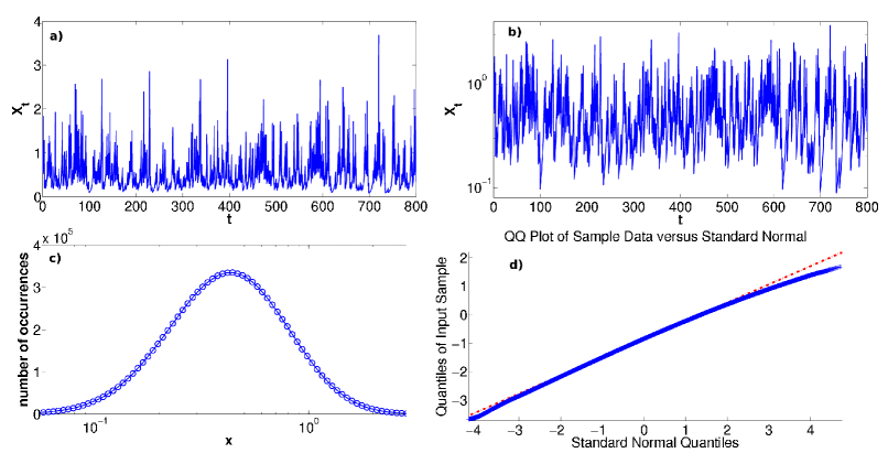
Figure 1: Plots of realizations and histograms of one-state system, see description in text for more detail.

4 Moment closure and convexity — Multiple states

We now extend the results of the previous section to the case where there are multiple states, i.e., $\left|{\mathcal{{Q}}}\right|>1$. The argument behind the method used here is the same as before: when we write down the moment equations, if we can show that if the right-hand side of the evolution equation for each moment has a term of higher degree, and this term has a negative coefficient, then the previous approach works as well. As before, we will assume that our state space is the positive reals, and that our reset maps are linear, i.e. $\psi_{kl}(x)=\gamma_{kl}x$.

The main results of this section are Theorems 4.3 and 4.4; the former gives sufficient conditions for the moment flow system to have bounded orbits, and the latter gives sufficient conditions for the moment flow system to have unbounded orbits. The technique used in the proofs of these theorems is, in principle, the same as in the previous section: there we had a case where, in each equation, there was a term involving the higher-order moment with a negative coefficient. In this case, we will show that there is a term on the right-hand side that plays the same role as this negative coefficient, but in this case, since the $m$th moment is effectively a vector of length $\left|{\mathcal{{Q}}}\right|$, this will be a $\left|{\mathcal{{Q}}}\right|\times\left|{\mathcal{{Q}}}\right|$ matrix whose sign-definiteness will establish stability (or the lack thereof).

4.1 Moment flow equations

We recall

$$\mathcal{{L}}h(q,x)=f(q,x)\cdot\nabla_{x}h(q,x)+\sum_{q^{\prime}\in\mathcal{{Q}}}\lambda_{q^{\prime}}(q,x)\left(h(q^{\prime},\psi_{q^{\prime}}(q,x))-h(q,x)\right).$$ (11)

Let us define, for $\theta\in\mathcal{{Q}}$ and $m\in\mathbb{N}$,

$$h_{\theta}^{(m)}(q,x):=1_{\theta}(q)x^{m}=\delta_{q,\theta}x^{m},\quad\mu_{\theta}^{(m)}:=\mathbb{E}[h_{\theta}^{(m)}(Q_{t},X_{t})].$$

Note that

$$\sum_{\theta\in\mathcal{{Q}}}h_{\theta}^{(m)}=x^{m},\mbox{ and thus }\mu^{(m)}:=\sum_{\theta\in\mathcal{{Q}}}\mu_{\theta}^{(m)}=\mathbb{E}[X_{t}^{m}]$$

is the total $m$th moment of $X_{t}$. One can think of $\mu_{\theta}^{(m)}$ as the conditional $m$th moment of $X_{t}$, conditional on $Q_{t}=\theta$, times the probability that $Q_{t}=\theta$. We plug $h_{\theta}^{(m)}$ into (11), to obtain

$$\mathcal{{L}}h_{\theta}^{(m)}(q,x) =f(q,x)\cdot\nabla_{x}h_{\theta}^{(m)}(q,x)+\sum_{\ell\in\mathcal{{Q}}}\lambda_{\ell}(q,x)h_{\theta}^{(m)}(\ell,\psi_{\ell}(q,x))-\sum_{\ell\in\mathcal{{Q}}}\lambda_{\ell}(q,x)h_{\theta}^{(m)}(q,x)$$

$$=f(q,x)1_{\theta}(q)\cdot m\cdot x^{m-1}+\sum_{\ell\in\mathcal{{Q}}}\lambda_{\ell}(q,x)1_{\theta}(\ell)(\gamma_{q,\ell}x)^{m})-\sum_{\ell\in\mathcal{{Q}}}\lambda_{\ell}(q,x)1_{\theta}(q)x^{m}.$$

We plug in $(Q_{t},X_{t})$ for $(q,x)$ and take expectations for each of the three pieces separately.

$$\begin{split}&\mathbb{E}[\mathcal{{L}}h_{\theta}^{(m)}(Q_{t},X_{t})]\\ &\qquad=m\mathbb{E}[1_{\theta}(Q_{t})f(Q_{t},X_{t})X_{t}^{m-1}]+\mathbb{E}[\sum_{\ell\in\mathcal{{Q}}}\lambda_{\ell}(Q_{t},X_{t})\gamma_{Q_{t},\ell}^{m}1_{\theta}(\ell)X_{t}^{m}]-\mathbb{E}[\sum_{\ell\in\mathcal{{Q}}}\lambda_{\ell}(Q_{t},X_{t})1_{\theta}(Q_{t})X_{t}^{m}].\end{split}$$ (23)

The first and third terms in the right-hand side of (23) are more or less straightforward, but the second term can be simplified in the following manner:

$$\mathbb{E}\left[\sum_{\ell\in\mathcal{{Q}}}\lambda_{\ell}(Q_{t},X_{t})\gamma_{Q_{t},\ell}^{m}1_{\theta}(\ell)X_{t}^{m}\right] =\mathbb{E}[\lambda_{\theta}(Q_{t},X_{t})\gamma_{Q_{t},\theta}^{m}X_{t}^{m}]$$

$$=\sum_{\ell\in\mathcal{{Q}}}\mathbb{E}[1_{\ell}(Q_{t})\lambda_{\theta}(Q_{t},X_{t})\gamma_{\ell,\theta}^{m}X_{t}^{m}],$$

and thus we have

$$\begin{split}&\mathbb{E}[\mathcal{{L}}h_{\theta}^{(m)}(Q_{t},X_{t})]\\ &\quad=m\mathbb{E}[1_{\theta}(Q_{t})f(Q_{t},X_{t})X_{t}^{m-1}]+\sum_{\ell\in\mathcal{{Q}}}\mathbb{E}[1_{\ell}(Q_{t})\lambda_{\theta}(Q_{t},X_{t})\gamma_{Q_{t},\theta}^{m}X_{t}^{m}]-\sum_{\ell\in\mathcal{{Q}}}\mathbb{E}\left[\lambda_{\ell}(Q_{t},X_{t})1_{\theta}(Q_{t})X_{t}^{m}\right].\end{split}$$ (24)

Example 4.1.

The general formula (24) is a bit complicated to parse, therefore we first work out a particular test case. Assume that all of the functions involved are linear, i.e.

$$f(q,x)=\alpha_{q}x,\quad\lambda_{\ell}(q,x)=\beta_{q,\ell}x,\quad\psi_{\ell}(q,x)=\gamma_{q,\ell}x,$$

then we obtain

$$\mathbb{E}[\mathcal{{L}}h_{\theta}^{(m)}(Q_{t},X_{t})]=m\alpha_{\theta}\mathbb{E}[1_{\theta}(Q_{t})X_{t}^{m}]+\sum_{\ell\in\mathcal{{Q}}}\beta_{\ell,\theta}\gamma_{\ell,\theta}^{m}\mathbb{E}\left[1_{\ell}(Q_{t})X_{t}^{m+1}\right]-\sum_{\ell\in\mathcal{{Q}}}\beta_{\theta,\ell}\mathbb{E}\left[1_{\theta}(Q_{t})X_{t}^{m{\color[rgb]{0,0,1}+1}}\right],$$

or

$$\frac{d}{dt}\mu_{\theta}^{(m)}(t)=m\alpha_{\theta}\mu_{\theta}^{(m)}(t)+\sum_{\ell\in\mathcal{{Q}}}\beta_{\ell,\theta}\gamma_{\ell,\theta}^{m}\mu_{\ell}^{(m+1)}(t)-\sum_{\ell\in\mathcal{{Q}}}\beta_{\theta,\ell}\mu_{\theta}^{(m+1)}(t).$$ (25)

Compare (25) to (18) and notice that it has much the same form: the function we differentiate appears first with a positive coefficient, also we have two terms of one higher degree with alternating signs, and the positive term has a $\gamma$ in it. What is different, and what makes this more complicated, is that the positive term of higher degree depends on the moments in different discrete states. So, while we will be able to use a Jensen-like argument to get boundedness, we have to be more careful, since we do not know that there is any relationship between $\mu_{q}^{(m)}$ and $\mu_{q^{\prime}}^{(m+1)}$ from just convexity — and thus we need to consider the entire vector $\{\mu_{q}^{(m)}\}_{q\in\mathcal{{Q}}}$.

Definition 4.2.

Let $X_{t}=\mathsf{SHS}(\mathcal{{Q}},\mathcal{{P}},\Lambda,\Psi,F)$. Let ${\mathsf{deg}}(\Lambda)=\max_{kl}{\mathsf{deg}}(\lambda_{kl})$, and define $\beta_{kl}$ as the coefficient of the term of degree ${\mathsf{deg}}(\Lambda)$ in $\lambda_{kl}(x)$, with the convention that $\beta_{kl}=0$ if ${\mathsf{deg}}(\lambda_{kl})<{\mathsf{deg}}(\Lambda)$. Then the top matrix of degree $m$ of the system is the matrix $M^{(m)}$ with coefficients

$$M^{(m)}_{kl}=\begin{cases}\gamma^{m}_{lk}\beta_{lk},&k\neq l,\\ -\sum_{l\in\mathcal{{Q}}}\beta_{kl},&k=l.\end{cases}$$

4.2 Theorems for stability

Theorem 4.3 (Bounded moments).

Assume that $\mathcal{{P}}=\mathbb{R}^{+}$, and let $X_{t}=\mathsf{SHS}(\mathcal{{Q}},\mathcal{{P}},\Lambda,\Psi,F)$. If ${\mathsf{deg}}(F)\leq{\mathsf{deg}}(\Lambda)$ and all of the eigenvalues of $M^{(m)}$ are negative, then the orbit of the total $m$th moment $\mu^{(m)}$ is bounded under the moment flow equations; in particular, if $M^{(m)}$ has negative spectrum for all $m\geq 1$, then all of the moments have bounded orbits.

Proof.

Let us first consider the case where all of the functions are linear, as in Example 4.1. Writing the vector $\mu^{(m)}=\{\mu_{q}^{(m)}\}_{q}$, we can write (25) as

$$\frac{d}{dt}\mu^{(m)}=mA\mu^{(m)}+M^{(m)}\mu^{(m+1)},$$ (26)

where $A$ is the diagonal matrix with $A_{qq}=\alpha_{q}$. Note that every entry in $A$ is positive, so the flow is linearly unstable at the origin.

However, also note that if $\mu^{(m)}\gg 1$, then $\mu^{(m+1)}\gg\mu^{(m)}$ by Jensen, which means that (26) is dominated by the second term. More precisely, if we assume that $\mu_{q}^{(m)}>1/\epsilon$ for all $q$, then $\mu_{q}^{(m+1)}>1/\epsilon^{1/m}\mu_{q}^{(m)}$, and thus we can write

$$\epsilon^{1/m}\frac{d}{dt}\mu^{(m)}\leq\epsilon^{1/m}A\mu^{(m)}+M^{(m)}\mu^{(m)}.$$ (27)

For $\epsilon$ sufficiently small, the first term is dominated. Since $M^{(m)}$ has negative spectrum, the flow $\dot{z}=M^{(m)}z$ is such that all $z(t)$’s in the positive octant will asymptotically approach the origin, and, moreover, this is structurally stable to a sufficiently small perturbation by the Hartman–Grobman Theorem. Thus, for $\epsilon$ small enough, all orbits are attracted to the origin, which means that (26) is inflowing on any ball of sufficiently large radius. Thus (26) has bounded orbits.

Now we consider the general $f,\lambda$ (recall that we assume throughout that $\psi_{k}(q,x)=\gamma_{qk}x$. Let us write

$$f(q,x) =\sum_{a=1}^{A_{q}}\alpha_{a,q}x^{a},$$

$$\lambda_{k}(q,x) =\sum_{b=1}^{B_{q,k}}\beta_{b,qk}x^{b}.$$

Then, plugging into (24), we have

$$\mathbb{E}[1_{\theta}(Q_{t})f(Q_{t},X_{t})X_{t}^{m-1}] =\mathbb{E}[1_{\theta}(Q_{t})\sum_{a=1}^{A_{Q_{t}}}\alpha_{a,Q_{t}}X_{t}^{a}X_{t}^{m-1}]$$

$$=\sum_{a=1}^{A_{\theta}}\alpha_{a,\theta}\mathbb{E}[1_{\theta}(Q_{t})X_{t}^{a+m-1}]=\sum_{a=1}^{A_{\theta}}\alpha_{a,\theta}\mu_{\theta}^{(a+m-1)},$$

$$\mathbb{E}\left[1_{\theta}(\ell)\gamma_{\ell,\theta}^{m}\lambda_{\theta}(\ell,X_{t})X_{t}^{m}\right] =\mathbb{E}\left[1_{\theta}(\ell)\gamma_{\ell,\theta}^{m}\sum_{b=1}^{B_{\ell,\theta}}\beta_{b,\ell\theta}X_{t}^{b}X_{t}^{m}\right]=\sum_{b=1}^{B_{\ell\theta}}\gamma_{\ell,\theta}^{m}\beta_{b,\ell\theta}\mu_{\ell}^{(b+m)},$$

$$\mathbb{E}\left[\lambda_{\ell}(Q_{t},X_{t})1_{\theta}(Q_{t})X_{t}^{m}\right] =\mathbb{E}\left[\sum_{b=1}^{B_{Q_{t},\ell}}\beta_{b,Q_{t}\ell}X_{t}^{b}X_{t}^{m}\right]=\sum_{b=1}^{B_{\theta,\ell}}\beta_{b,\theta\ell}\mu_{\theta}^{(b+m)},$$

or

$$\frac{d}{dt}\mu_{\theta}^{(m)}=m\sum_{a=1}^{A_{\theta}}\alpha_{a,\theta}\mu_{\theta}^{(a+m-1)}+\sum_{b=1}^{B_{\ell,\theta}}\gamma_{\ell,\theta}^{m}\beta_{b,\ell\theta}\mu_{\ell}^{(b+m)}-\sum_{b=1}^{B_{\theta,\ell}}\beta_{b,\theta\ell}\mu_{\theta}^{(b+m)}.$$ (28)

Recalling the definition of $M^{(m)}$, this means that the last two terms in (28) can be written as $M^{(m)}\mu^{(m+{\mathsf{deg}}(\Lambda))}$ — note that the definition of $M^{(m)}$ includes, by design, only those coefficients that are the same degree as the highest possible degree of all $\lambda_{kl}$. Thus (28) can be written as

$$\frac{d}{dt}\mu_{\theta}^{(m)}=\sum_{\ell=m-1}^{m+{\mathsf{deg}}(\Lambda)-1}A_{\ell}\mu^{(\ell)}+M^{(m)}\mu^{(m+{\mathsf{deg}}(\Lambda))},$$ (29)

and clearly the same sort of asymptotic analysis done for the linear case works here as well, since the first term is strictly dominated in powers by the last. ∎

Theorem 4.4 (Unbounded moments).

Let $\mathcal{{P}}=\mathbb{R}^{+}$ and $X_{t}=\mathsf{SHS}(\mathcal{{Q}},\mathcal{{P}},\Lambda,\Psi,F)$.

1. If ${\mathsf{deg}}(F)\leq{\mathsf{deg}}(\Lambda)$, and

   1. $\left\langle{{M^{(m)}x}},{{y}}\right\rangle>0$ for all $x,y$ in the positive octant, or

   2. there exist $k,l$ such that $\min(M_{kl}^{(m)},M_{lk}^{(m)})>\max(|M_{kk}^{(m)}|,|M_{ll}^{(m)}|)$;

   then the orbit of the total $m$th moment $\mu^{(m)}$ is unbounded under the moment flow equations;

2. If ${\mathsf{deg}}(F)>{\mathsf{deg}}(\Lambda)$, then for $m$ sufficiently large, all $m$th moments have unbounded orbits under the moment flow equations.

3. If ${\mathsf{deg}}(F)>{\mathsf{deg}}(\Lambda)+1$, then all $m$th moments have unbounded orbits under the moment flow equations.

Proof.

Again consider (29). First assume that $\left\langle{{M^{(m)}x}},{{y}}\right\rangle>0$ for all $x,y$ in the positive octant. Since all of the $A_{\ell}$ in that formula are diagonal with positive entries, it follows directly that the vector field is outflowing on every circle.

On the other hand, assume that there exists a $k,l$ such that $\min(M_{kl}^{(m)},M_{lk}^{(m)})>\max(M_{kk}^{(m)},M_{ll}^{(m)})$. Without loss of generality by renumbering, assume that we have $\min(M_{12}^{(m)},M_{21}^{(m)})>\max(|M_{11}^{(m)}|,|M_{22}^{(m)}|)$. Let us again consider the linear case, as the nonlinear case is the same. We have

$$\frac{d}{dt}\mu_{1}^{(m)} =m\alpha_{1}\mu_{1}^{(m)}+M_{12}^{(m)}\mu_{2}^{(m+1)}-|M_{11}^{(m)}|\mu_{1}^{(m+1)},$$

$$\frac{d}{dt}\mu_{2}^{(m)} =m\alpha_{2}\mu_{2}^{(m)}+M_{21}^{(m)}\mu_{1}^{(m+1)}-|M_{22}^{(m)}|\mu_{2}^{(m+1)}.$$

Writing $\nu^{(m)}=e^{-mAt}\mu^{(m)}$, where $A=\mathrm{diag}(\alpha_{1},\alpha_{2})$, we have

$$\frac{d}{dt}\nu_{1}^{(m)} =M_{12}^{(m)}\mu_{2}^{(m+1)}-|M_{11}^{(m)}|\mu_{1}^{(m+1)},$$

$$\frac{d}{dt}\nu_{2}^{(m)} =M_{21}^{(m)}\mu_{1}^{(m+1)}-|M_{22}^{(m)}|\mu_{2}^{(m+1)}.$$

and thus

$$\frac{d}{dt}(\nu_{1}^{(m)}+\nu_{2}^{(m)})=(M_{21}^{(m)}-|M_{11}^{(m)}|)\mu_{1}^{(m+1)}+(M_{12}^{(m)}-|M_{22}^{(m)}|)\mu_{2}^{(m+1)}>0,$$

so that this sum is always growing, and thus the corresponding sum for $\mu^{(m)}$ grows at least exponentially.

Now consider the case where ${\mathsf{deg}}(F)={\mathsf{deg}}(\Lambda)+1$ — this implies that the first term in (28) is of the same degree, than all of the other terms. Thus (28) looks like

$$\frac{d}{dt}\mu_{m}^{(m)}=A\mu^{(m+{\mathsf{deg}}(\Lambda))}+M^{(m)}\mu^{(m+{\mathsf{deg}}(\Lambda))}+O(\mu^{(m+{\mathsf{deg}}(\Lambda)-1)},$$

and since the diagonals of $A$ grow linearly in $m$, for sufficiently large $M$, all of the coefficients of $A+M^{(m)}$ are positive, and thus the flow has unbounded orbits.

Finally, if ${\mathsf{deg}}(F)>{\mathsf{deg}}(\Lambda)+1$, then (28) becomes

$$\frac{d}{dt}\mu_{m}^{(m)}=A\mu^{(m+{\mathsf{deg}}(F)-1)}+M^{(m)}\mu^{(m+{\mathsf{deg}}(\Lambda))}+O(\mu^{(m+{\mathsf{deg}}(F)-2)},$$

where the dominant term is the $A$ term, which is diagonal with positive diagonals for all $m$. ∎

4.3 Examples and corollaries

We have shown above that as long as $M^{(m)}$ has all negative eigenvalues, the $m$th moment is stable. First we show:

Corollary 4.5.

If $0<\gamma_{kl}<1$ for all $k,l$, then $\mathbb{E}[X_{t}^{m}]$ is bounded above for all $t$ and for all $m$.

Proof.

From Theorem 4.3, all we need to show is that $M^{(m)}$ has all negative eigenvalues. Recall that

$$M^{(m)}_{kl}=\begin{cases}\gamma^{m}_{lk}\beta_{lk},&k\neq l,\\ -\sum_{l\in\mathcal{{Q}}}\beta_{kl},&k=l.\end{cases}$$

By the Gershgorin Circle Theorem, the eigenvalues of $M^{(m)}$ are contained in the union of the $\left|{\mathcal{{Q}}}\right|$ balls

$$B_{k}:=B\left(M^{(m)}_{kk},\sum_{l=1}^{\left|{\mathcal{{Q}}}\right|}\left|{M^{(m)}_{kl}}\right|\right),$$

i.e., the $k$th ball is centered at the $k$th diagonal coefficient, and whose radius is given by the sum of the absolute values of the off-diagonal terms. Since $\gamma_{kl}<1$, and thus $\gamma_{kl}^{m}<1$, we have

$$\sum_{l=1}^{\left|{\mathcal{{Q}}}\right|}\left|{\gamma_{kl}^{m}M^{(m)}_{kl}}\right|<\sum_{l=1}^{\left|{\mathcal{{Q}}}\right|}\left|{M^{(m)}_{kl}}\right|=\left|{M^{(m)}_{kk}}\right|.$$

∎

Example 4.6.

Let us assume that $\left|{\mathcal{{Q}}}\right|=2$, so that

$$M^{(1)}=\left(\begin{array}[]{cc}-\beta_{12}&\beta_{21}\gamma_{21}\\ \beta_{12}\gamma_{12}&-\beta_{21}\\ \end{array}\right).$$

We have $\mathrm{Tr}M^{(1)}=-\beta_{12}-\beta_{21}<0$, and $\det M^{(1)}=\beta_{12}\beta_{21}(1-\gamma_{12}\gamma_{21})$. It is not hard to see that the resulting linear system is a saddle if $\gamma_{12}\gamma_{21}>1$, and a sink if $\gamma_{12}\gamma_{21}<1$. By Theorem 4.3, if $\gamma_{12}\gamma_{21}<1$ this means that $\mathbb{E}[X_{t}]$ is bounded above. Of course, note that the stability condition for $M^{(m)}$ is $\gamma_{12}^{m}\gamma_{21}^{m}<1$, and thus stability of the first moment implies stability of all higher moments. As we see below, this is a special case only if $\left|{\mathcal{{Q}}}\right|=2$.

In fact, one can get at this result from other means: notice that in the $2\times 2$ case, all jumps $1\to 2$ are immediately followed by a jump $2\to 1$, and the aggregate effect of these jumps is to multiply by $\gamma_{1}\gamma_{2}$. Thus it is clear that the necessary and sufficient condition for stability is that this product be less than one.

One of the interesting observations made in the previous example is that we do not require that all $\gamma_{kl}$ be less than one. But for general $\left|{\mathcal{{Q}}}\right|>2$, if we choose one or more of the $\gamma_{kl}>1$, then we will see some unbounded moments, as in the following example.

Example 4.7.

Consider the symmetric case where we choose $\beta_{kl}=1$ for all $k,l$, and choose $\gamma_{12}>1$, but $\gamma_{13},\gamma_{23}<1$, so that we have

$$M^{(m)}=\left(\begin{array}[]{ccc}-2&\gamma_{12}^{m}&\gamma_{13}^{m}\\ \gamma_{12}^{m}&-2&\gamma_{23}^{m}\\ \gamma_{13}^{m}&\gamma_{23}^{m}&-2\end{array}\right).$$

If we further choose $\gamma_{12}+\gamma_{13}<2$ and $\gamma_{12}+\gamma_{23}<2$, then again by Gershgorin theorem, it follows that $M^{(1)}$ has all negative eigenvalues, and by Theorem 4.3, the moment flow is stable at first order.

Since $\gamma_{12}>1$, then for some $m>1$, $\gamma_{12}^{m}>2$, and by Theorem 4.4, the moment flow is unstable at $m$th order. Thus we have a scenario where $\mathbb{E}[X_{t}]$ is bounded above for all time, but $\mathbb{E}[X_{t}^{m}]$ grows without bound.

We saw in Example 4.7 that we can construct a process where the mean is bounded above, but some higher moments grow without bound. In fact, it should be clear that if there is a pair $(k,l)$ with $\gamma_{kl}>1$ and $\gamma_{lk}>1$, then this will generically occur: for sufficiently large $m$, the $m$th moment is unstable. This can lead to some counter-intuitive effects, as seen by the following example.

Example 4.8.

Consider the case where $\left|{\mathcal{{Q}}}\right|=N$, $\gamma_{12}=\gamma_{21}>N-1$, and all of other the $\gamma_{kl}$ are arbitrarily small (for the purposes of this argument, set them to zero), so that if the system ever enters a state other than $1$ or $2$, then $X_{t}$ is set to zero. Let all $\beta_{kl}=1$, so that the jump rates are all the same. Specifically, this means that whenever there is a jump, the next discrete state is chosen uniformly in the others. Start with $Q_{0}=1,X_{0}=1$. The probability of never leaving $Q_{t}\in\{1,2\}$ after the first $k$ jumps is then $(N-1)^{-k}$, but the multiplier from these transitions is $\gamma_{12}^{k}$, so that $\mathbb{E}[X_{T_{k}}]$ grows exponentially, even if $\mathbb{P}(X_{T_{k}}>0)$ is shrinking exponentially.

Similarly, we could see that if we choose $\gamma_{12}<N-1<\gamma_{12}^{2}$, then $\mathbb{E}[X_{t}]$ would decay exponentially, but $\mathbb{E}[X_{t}^{2}]$ would grow exponentially, and similarly for higher moments.

In short, this says that to obtain a moment instability, all one needs is two states exchanging back and forth, as long as their multipliers are large enough, even if the probability of this sequence of switching is small — which is the content of Part 1 of Theorem 4.4.

When we have a probability distribution with some moments finite and others infinite, this is called a heavy-tailed distribution (see [36, 37] for examples in dynamical systems). The canonical example of a heavy-tailed distribution is one whose tail decays asymptotically as a power law, and as such, are typically associated with critical phenomena in statistical physics [38, 39, 40, 41, 42, 43, 44]. In fact, if we assume that $p(x)$ is the distribution of the process in equilibrium, that $p(x)\sim x^{-\alpha}$ as $x\to\infty$, and $X_{\infty}$ is a realization of this distribution, then

$$\mathbb{E}[X_{\infty}^{m}]=\int_{0}^{\infty}x^{m}p(x)\,dx\approx\int_{x_{*}}^{\infty}x^{m-\alpha}\,dx$$

will converge iff $m-\alpha<1$. From this we deduce that if $\alpha\in(m,m-1)$, then $\mathbb{E}[X_{\infty}^{m}]<\infty$ but $E[X_{\infty}^{m+1}]=\infty$. We will in fact show numerical evidence of power law tails in SHS dynamics in the next section, which leads us to conjecture that the extreme case of Example 4.8 above is atypical.

4.4 Numerical results

In Figure 2, we plot the results of a Monte Carlo simulation for a two-state SHS. We simulate $10^{3}$ realizations of this system, and each realization was integrated until $10^{4}$ jumps had occurred.

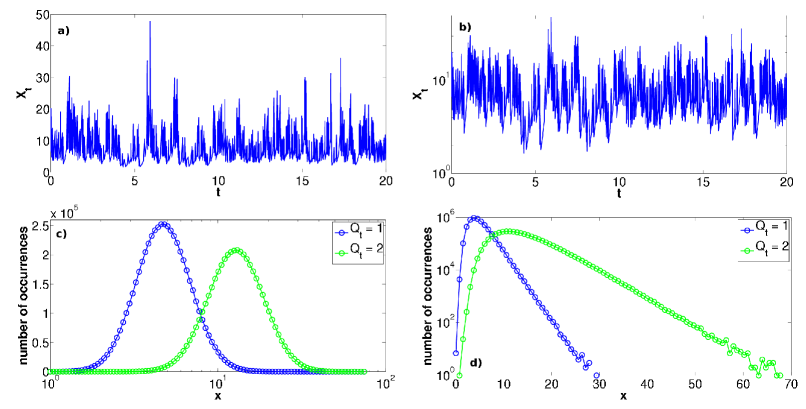
Figure 2: Two-state case that is moment stable, with exponential tails. See text for description and explanation.

Here, we have chosen

$$f(q,x)=\alpha_{q}x^{2},\quad\lambda_{q^{\prime}}(q,x)=\beta_{q,q^{\prime}}x^{2},$$

where $q,q^{\prime}\in\{1,2\}$, and as always the resets are $\gamma_{q,q^{\prime}}x$. We chose the $\alpha,\beta,\gamma$ as follows:

$$\alpha=\left(\begin{array}[]{c}2\\ 1\end{array}\right),\quad\beta=\left(\begin{array}[]{cc}0&1\\ 1&0\end{array}\right),\quad\gamma=\left(\begin{array}[]{cc}0&2\\ 1/3&0\end{array}\right).$$

Since $\gamma_{12}\gamma_{21}<1$, by the results above all moments are stable, and this is what we observe numerically.

In Figures 2a and  2b, we plot a single trajectory of the system (in (a) we have plotted this in a linear-linear scale, and in (b) we plot the same data in a linear-log scale). We have only plotted a subset of the entire realization here; the full realization of $10^{4}$ jumps goes until approximately $t=254$, and here we are only plotting $812$ jumps and cutting off at $t=20$ in order to see more structure.

In Figure 2c,d, we plot aggregate histograms of $X_{t}$, each plot uses $0.5\times 10^{6}$ datapoints. Recall that each realization of the process was run for $10^{4}$ jumps; we discarded the first half of these for each realization, giving $0.5\times 10^{3}$ points, then aggregated across realizations. The first observation is that the distribution is bimodal, and this is due to the up-and-down jumps: since $\gamma_{12}>1$ and $\gamma_{21}<1$, we expect the typical value of $X_{t}$ to be much higher when $Q_{t}=2$ than when it equals one. We separate out the data by the value of $Q_{t}$. In Figure 2c, we plot on a log-linear scale, and it is pretty apparent to the eye that the distributions for $X_{t}$, conditioned on $Q_{t}$, are close to log-normal, as was the distribution in the one-state case (q.v. Figure 1). We checked this observations with QQ-plots (not presented here) and saw the same phenomenon observed in Figure 1. In (d), we plot a histogram on a linear-log scale, and the data shows an exponential tail, consistent with the prediction that all of the moments are uniformly bounded above.

In Figure 3, we plot the results of a Monte Carlo simulation for a three-state SHS. Again, we simulate $10^{3}$ realizations of this system, and each realization was integrated until $10^{4}$ jumps had occurred.

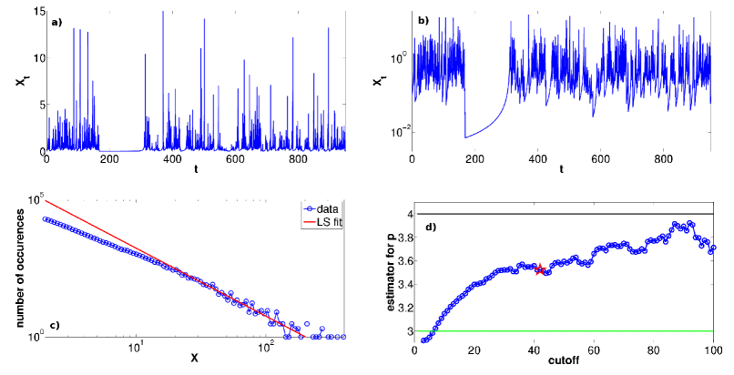
Figure 3: Three-state case that is marginally moment stable. See text for description and explanation.

Here we have chosen

$$f(q,x)=\alpha_{q}x^{2},\quad\lambda_{q^{\prime}}(q,x)=\beta_{q,q^{\prime}}x^{2},$$

where $q,q^{\prime}\in\{1,2,3\}$, and as always the resets are $\gamma_{q,q^{\prime}}x$. We chose the $\alpha,\beta,\gamma$ as follows:

$$\alpha=\left(\begin{array}[]{c}2\\ 1\\ 3\end{array}\right),\quad\beta=\left(\begin{array}[]{ccc}0&1&1\\ 1&0&1\\ 1&1&0\end{array}\right),\quad\gamma=\left(\begin{array}[]{ccc}0&1.3&0.3\\ 1.3&0&0.2\\ 0.3&0.2&0\end{array}\right).$$

This means that

$$M^{(m)}=\left(\begin{array}[]{ccc}-2&(1.3)^{m}&(0.3)^{m}\\ (1.3)^{m}&-2&(0.2)^{m}\\ (0.3)^{m}&(0.2)^{m}&-2\end{array}\right),$$

and one can see that

$$(1.3)^{2}+(0.3)^{2}<2,\quad(1.3)^{3}>2,$$

so by the theorems above, we have that the first two moments are stable and the third is not — thus as $t\to\infty$, $\mathbb{E}[X_{t}]<\infty$ and $\mathbb{E}[X_{t}^{2}]<\infty$, but $\mathbb{E}[X_{t}^{3}]$ grows without bound. Thus, if we see a power-law tail in the distribution, we expect it to decay somewhere as $x^{-p}$ with $p$ between $3$ and $4$.

In Figure 3(a,b), we again plot a single trajectory of the system (in (a) we have plotted this in a linear-linear scale, and in (b) we plot the same data in a linear-log scale). We see the wide variety of spatial scales in the linear plot, and the “intermittent” structure of the process in the log case — sometimes the system can be kicked quite low, and takes a while to climb out of it. Recall that the ODE is quadratically nonlinear, so if $X_{t}$ ever happens to become small, it will take a long time to leave a neighborhood of zero.

In Figure 3c, we plot an aggregate histogram of $0.5\times 10^{6}$ datapoints on a log-log scale. Recall that each realization of the process was run for $10^{4}$ jumps; we discarded the first half of these for each realization, giving $0.5\times 10^{3}$ points, then aggregated across realizations. We see from eye that it looks to have a power law structure for large $x$, and we also plot the least squares linear fit to the higher half of the data. This slope is given as $p=-2.4797\pm 0.0112$, which seems to contradict our assessment from above. However, it should be pointed out that trying to match a power law fit by least squares on a log-log plot gives in general a bad estimator [45, 46], so we reevaluate our analysis of the decay.

We use the procedure laid out in [46] as follows: given a data set $\{x_{i}\}$, first decide a cutoff $x_{\mathsf{min}}$, let $n=\#\{x_{i}>x_{\mathsf{min}}\}$, and this gives the estimator

$$\hat{p}=1+\frac{n}{\sum_{i=1}^{n}\log(x_{i}/x_{\mathsf{min}})\mathbf{1}(x_{i}>x_{\mathsf{min}})}.$$

In Figure 3d, we plot $\hat{p}$ for all cutoffs in the range $[1,100]$, and we see that as long as we use a cutoff of about 10 or more, this is consistent with the theoretical prediction. [The horizontal lines in Figure 3(d) are the bounds given by the analysis.] We plot by a red star the value that is given by the “best” estimator, determined in the following manner: for each choice of $x_{\mathsf{min}}$, we compare the empirical data with the theoretical distribution assuming that our estimate of $\hat{p}$, then measure the closeness of these distributions using the Kolmogorov-Smirnoff (KS) distance. The best fit was given by a cutoff of $42$, with a estimator of $\hat{p}=3.523$, and a KS distance between the theoretical and empirical distributions of $7.78\times 10^{-3}$.

5 Finite-time blowups

In this section, we will again return to the one-state case considered in Section 3. It was shown there that as long as ${{\mathsf{deg}}(\lambda)}\geq{{\mathsf{deg}}(f)}$, the stochastic process is “well-behaved”, i.e. as $t\to\infty$, all of the moments are finite. In particular, it is not possible for the process to escape to infinity in finite time.

However, in general, if the driving ODE is nonlinear, then it is certainly possible that the process escapes to infinity in finite time (these events are usually called finite-time blowups in the dynamical systems literature, or explosions in the stochastic process literature). We examine these behaviors in this section.

Definition 5.1.

Let us denote by $T_{n}$ the times where the SHS has jumps. We say that a realization of an SHS has a finite-time blowup if either of two conditions hold:

1. $T_{\infty}:=\lim_{n\to\infty}T_{n}<\infty,$

2. the solution of the continuous part becomes infinite between any two jump times.

We will refer to the two types of blowup as Type I and Type II.

Remark 5.2.

What we are calling a “Type I” blowup is the type of behavior that is typically called an explosion for stochastic processes. These are common for countable Markov chains where the jump rates can grow sufficiently fast. What we call a “Type II” blowup is very much like what is called a finite-time blowup in the differential equations literature — in this context, since the jump never occurs, it is the same as an ODE going to infinity.

The results of this section can be summarized as follows: let $X_{t}=\mathsf{SHS}(f,\lambda,\gamma)$ with ${{\mathsf{deg}}(f)}>1$; then, we have the following two cases:

1. If ${{\mathsf{deg}}(\lambda)}<{{\mathsf{deg}}(f)}-1$, then $X_{t}$ will have a Type II blowup with probability one for any initial condition;

2. if ${{\mathsf{deg}}(\lambda)}={{\mathsf{deg}}(f)}-1$, then, depending on the leading coefficients of $f$ and $\lambda$, the system exhibits various behaviors, summarized in Theorem 5.4 below. In particular, in some parameter regimes it exhibits Type I blowups almost surely, and the remaining regimes it does not exhibit Type I blowups almost surely. If ${{\mathsf{deg}}(f)}=1$, then the system cannot blowup, since linear flows are well-defined for all time. However, as we show below, in the parameter range where the nonlinear systems exhibit finite-time blowups, the linear system still go to infinity but take an infinite amount of time to do so, exhibiting in some sense an “infinite-time blowup”.

We consider these two cases in the subsections below.

5.1 Case C1: ${{\mathsf{deg}}(\lambda)}<{{\mathsf{deg}}(f)}-1$

We first consider the case where ${{\mathsf{deg}}(\lambda)}<{{\mathsf{deg}}(f)}-1$. We show here that any such system has a Type II blowup — basically, the ODE goes to infinity too fast for the jump rates to catch up.

Theorem 5.3.

Let $X_{t}=\mathsf{SHS}(f,\lambda,\psi)$, and assume that ${{\mathsf{deg}}(\lambda)}<{{\mathsf{deg}}(f)}-1$. Then $X_{t}$ has a Type II blowup with probability one for any initial condition.

Proof.

Using standard ODE arguments, if

$$\frac{d}{dt}\varphi^{t}(x)=f(\varphi^{t}(x)),$$

where $f(x)$ is a positive polynomial of degree ${{\mathsf{deg}}(f)}>1$, then $\varphi^{t}(x)$ has a finite-time singularity at some $t^{*}<\infty$, and, moreover, in a (left) neighborhood of this point, we have

$$\varphi^{t}(x)\sim C(t-t^{*})^{1/(1-{{\mathsf{deg}}(f)})}.$$

If ${{\mathsf{deg}}(\lambda)}<{{\mathsf{deg}}(f)}-1$, then $0>{{\mathsf{deg}}(\lambda)}/(1-{{\mathsf{deg}}(f)})>-1$. Writing $\lambda(x)=\beta x^{{\mathsf{deg}}(\lambda)}+O(x^{{{\mathsf{deg}}(\lambda)}-1})$, we have that $\lambda(\varphi^{s}(x))$ is integrable near this singular point, i.e.

$$\int_{t_{0}}^{t^{*}}\lambda(\varphi^{s}(x))\,ds<\infty.$$

Since any exponential has support on the whole real axis, this and (4) means that starting at any initial condition, the probability of the ODE having a singularity before jumps is positive, i.e.

$$\mathbb{P}\left(S_{n}>\int_{t_{0}}^{t^{*}}\beta(\varphi^{s}(x))\,ds\right)>0,$$

and the system has a Type II blowup with positive probability. Since the process is Markov, irreducible on $\mathbb{R}^{+}$, and aperiodic, it follows that the system has a Type II blowup with probability one. ∎

5.2 Case C2: ${{\mathsf{deg}}(\lambda)}={{\mathsf{deg}}(f)}-1$

This case is much more complicated than the previous one for various reasons, not the least of which being that the behavior depends on the coefficients of the functions $f$ and $\lambda$. The behavior is summarized in the following theorem:

Theorem 5.4.

Let $X_{t}=\mathsf{SHS}(f,\lambda,\gamma)$, where

$$f(x)=\alpha x^{k+1}+O(x^{k}),\quad\lambda(x)=\beta x^{k}+O(x^{k-1}),$$ (30)

$k\geq 1$ (so that the ODE is superlinear), and all of the coefficients of both polynomials are positive. Then:

1. if $\gamma>e^{-\alpha/\beta}$, then $X_{t}$ has Type I blowups almost surely;

2. if $1-\alpha/\beta<\gamma<e^{-\alpha/\beta}$, then $X_{t}\to 0$ in probability, even though $\mathbb{E}[X_{t}]\to\infty$ as $t\to\infty$;

3. if $\gamma<1-\alpha/\beta$, then $X_{t}\to 0$, both in $L^{1}$ and almost surely.

In particular, $X_{t}$ will not have Type II blowups.

Finally, if we assume a linear ODE, i.e. $X_{t}=\mathsf{SHS}(\alpha x,\beta,\gamma)$, then the conclusions above are all true except for #1, in which case we have that $X_{t}\to\infty$ a.s., but $X_{t}<\infty$ w.p. 1 for any finite $t$.

The way we proceed to prove this is as follows. We first compute a recurrence relation when $f,\lambda$ are assumed to be pure monomials, and then show that this recurrence relation has growth properties that correspond to the three types of convergence above, in the appropriate parameter regimes. Finally, we prove a monotonicity theorem that allows us to extend the calculation for monomials to general polynomials.

Proposition 5.5.

If $X_{t}=\mathsf{SHS}(f,\lambda,\gamma)$ with ${{\mathsf{deg}}(\lambda)}={{\mathsf{deg}}(f)}-1$, then the probability of a Type II blowup is zero for any initial condition.

Proof.

Since ${{\mathsf{deg}}(\lambda)}={{\mathsf{deg}}(f)}-1$, then $\lambda(\varphi^{t}(x))\sim 1/t$ in a neighborhood of the singularity (see the beginning of the proof of Proposition 5.3 for more detail), so that

$$\int_{t_{0}}^{t^{*}}\lambda(\varphi^{s}(x))\,ds=\infty,$$

and a Type II blowup is not possible. ∎

Lemma 5.6.

Let $X_{t}=\mathsf{SHS}(f,\lambda,\gamma)$ with $f(x)=\alpha x^{k+1}$ and $\lambda(x)=\beta x^{k}$. Then

$$X_{T_{n}}=\gamma e^{(\alpha/\beta)S_{n}}X_{T_{n-1}},$$

where $S_{n}$ are iid unit-rate exponential random variables.

Proof.

It is not hard to check that

$$\varphi^{t}(x)=\frac{x}{(1-\alpha ktx^{k})^{1/k}},$$

and thus

$$\lambda(\varphi^{t}(x))=\frac{\beta x^{k}}{1-\alpha ktx^{k}}.$$

Therefore, we have

$$S_{n} =\int_{0}^{T_{n+1}-T_{n}}\lambda(\varphi^{s}(X_{T_{n}}))\,ds=\int_{0}^{T_{n+1}-T_{n}}\frac{\beta(X_{T_{n}})^{k}}{1-\alpha ks(X_{T_{n}})^{k}}\,ds$$

$$=\frac{-\beta}{\alpha k}\ln\left|{1-\alpha ks(X_{T_{n}})^{k}}\right|\Bigg{|}_{s=0}^{s=T_{n+1}-T_{n}}=\frac{-\beta}{\alpha k}\ln\left|{1-\alpha k(T_{n+1}-T_{n})(X_{T_{n}})^{k}}\right|.$$

From this, one can see that

$$1-\alpha k(T_{n+1}-T_{n})(X_{T_{n}})^{k}=e^{-\alpha/(\beta k)S_{n}}.$$ (31)

We then compute

$$\begin{split}X_{T_{n+1}}&=\gamma\varphi^{T_{n+1}-T_{n}}(X_{T_{n}})\\ &=\gamma\frac{X_{T_{n}}}{(1-\alpha k(T_{n+1}-T_{n})(X_{T_{n}})^{k})^{1/k}}=\gamma e^{\frac{\alpha}{\beta}S_{n}}X_{T_{n}}.\end{split}$$ (32)

∎

Lemma 5.7.

Let $S_{k}$ be iid unit rate exponentials and define

$$Z_{n}=\prod_{k=1}^{n}\gamma e^{(\alpha/\beta)S_{k}}.$$

Then:

1. if $\gamma>e^{-\alpha/\beta}$, then there exists a $\delta^{\prime}>0$ such that $\liminf_{n}e^{-\delta^{\prime}n}Z_{n}=\infty$ with probability one;

2. if $1-\alpha/\beta<\gamma<e^{-\alpha/\beta}$, then $Z_{n}\to 0$ in probability, even though $\mathbb{E}[Z_{n}]\to\infty$ as $t\to\infty$;

3. if $\gamma<1-\alpha/\beta$, then $Z_{n}\to 0$, both in $L^{1}$ and almost surely.

Proof.

Let us write $W_{k}=\gamma e^{(\alpha/\beta)S_{k}}$. Let us write $\mu=\mathbb{E}[W_{k}]$ and $\delta=\mathbb{E}[\log(W_{k})]$. We compute:

$$\mu=\gamma\mathbb{E}[e^{(\alpha/\beta)S_{k}}]=\gamma\int_{0}^{t}e^{(\alpha/\beta)t}e^{-t}\,dt=\frac{\gamma}{1-\alpha/\beta}.$$

We also have

$$\delta=\mathbb{E}\left[\frac{\alpha}{\beta}S_{k}+\log\gamma\right]=\frac{\alpha}{\beta}+\log\gamma.$$

Note then that the three conditions in this lemma correspond to $\delta>0$; $\delta<0$ and $\mu>1$; and $\mu<1$, respectively. (By Jensen’s inequality, we have

$$\mu=\mathbb{E}[W_{k}]=\mathbb{E}[e^{\log(W_{k})}]>e^{\mathbb{E}[\log(W_{k})]}=e^{\delta},$$

so clearly $\delta>0$ implies $\mu>1$, and these are the only three possibilities.)

First, we compute

$$\mathbb{E}[Z_{n}]=\mathbb{E}\left[\prod_{k=1}^{n}W_{k}\right]=\prod_{k=1}^{n}\mathbb{E}[W_{k}]=\mu^{n},$$

so clearly the expectation goes to zero (resp. $\infty$) if $\mu<1$ (resp. $\mu>1$). Since $Z_{n}\geq 0$ by definition, this implies that $Z_{n}\to 0$ both in $L^{1}$ and almost surely. This establishes claim #3 of the lemma.

Next, note that

$$Z_{n}=\exp(\log(Z_{n}))=\exp\left(\sum_{k=1}^{n}\log W_{k}\right)=\exp\left(\frac{\alpha}{\beta}\sum_{k=1}^{n}S_{k}+n\log\gamma\right).$$

From the Law of Large Numbers,

$$\sum_{k=1}^{n}\log W_{k}=n\mathbb{E}[\log W_{k}]\pm O(\sqrt{n})=n\left(\frac{\alpha}{\beta}+\log\gamma\right)\pm O(\sqrt{n}),$$

and if $\delta\neq 0$, this sum goes to $\pm\infty$ depending on the sign of $\delta$. More specifically, we can use Chernoff-type bounds [47, 48]: let $\delta>0$. Since

$$\mathbb{E}\left[\sum_{k=1}^{n}\log W_{k}\right]=n\delta,$$

the Chernoff bounds give

$$\mathbb{P}\left(\sum_{k=1}^{n}\log W_{k}<n\delta/2\right)<e^{-n\delta/8},$$

or

$$\mathbb{P}\left(Z_{n}<e^{n\delta/2}\right)<e^{-n\delta/8}.$$ (33)

In particular, this means that $Z_{n}$ grows faster than an exponential with probability exponentially close to one. For example, choose $0<\delta^{\prime}<\delta/2$. Now, if it is not true that $\liminf e^{-\delta^{\prime}n}Z_{n}=\infty$, this means that there exists $M>0$ and an infinite sequence $n_{1},n_{2},\dots,n_{k},\dots$ such that $e^{-\delta^{\prime}{n_{k}}}Z_{n_{k}}\leq M$. From (33), this event has probability zero. This proves claim #1 of the lemma.

Conversely, if $\delta<0$, then

$$\mathbb{P}\left(Z_{n}>e^{n\delta/2}\right)<e^{-n\delta/12},$$

or the infinite product goes to zero exponentially fast with probability exponentially close to one, which implies that $Z_{n}\to 0$ in probability. Thus, if $\delta<0$ and $\mu>1$, then we have that $Z_{n}\to 0$ in probability but $\mathbb{E}[Z_{n}]\to\infty$, proving claim #2 of the theorem. ∎

Lemma 5.8.

Let $X_{t}=\mathsf{SHS}(f,\lambda,\gamma)$ and $Y_{t}=\mathsf{SHS}(g,\mu,\gamma)$, and assume that

$$X_{0}\leq Y_{0},\quad g(x)\geq f(x),\quad\mu(x)\leq\lambda(x).$$ (34)

If $X_{t}(\omega)$ has a finite-time blowup, then so does $Y_{t}(\omega)$. Thus, the probability of $Y_{t}$ having a finite-time blowup is at least as large as $X_{t}$ having one, and so, for example, if $X_{t}$ has an a.s. finite-time blowup, then so does $Y_{t}$.

Conversely, if there exists an $M>0$ such that for all $x\leq M$, (34) holds, and $X_{0}\leq Y_{0}\leq M$, if $Y_{t}(\omega)\to 0$ as $t\to\infty$, then so does $X_{t}(\omega)$, and thus the probability of $X_{t}$ decaying to zero is at least as large as the probability that $Y_{t}$ does.

Proof.

We denote $T_{n}^{(X)}$ as the $n$th reset time for process $X_{t}$, and similarly for $T_{n}^{(Y)}$. Since $\mu\leq\lambda$, $T_{1}^{(Y)}\geq T_{1}{(X)}$. Together with the fact that $g\geq f$, this implies that $Y_{T_{1}^{(Y)}}\geq X_{T_{1}^{(X)}}$. Using induction, the random sequence $Y_{T_{n}^{(Y)}}$ dominates the sequence $X_{T_{n}^{(X)}}$ for any $\omega$, and the conclusions follow. ∎

Remark 5.9.

Said in words: if we make the vector field larger, or the rate smaller, then the system is more likely to blow up. Conversely, if we make the vector field smaller, or the rate larger, the system is more likely to go to zero.

Proof of Theorem 5.4. Let us first consider the case where $f$ and $\lambda$ are pure monomials, i.e., $f(x)=\alpha x^{k+1}$, $\lambda(x)=\beta x^{k}$. Let us first consider the case where $\gamma>e^{-\alpha/\beta}$. Using Lemmas 5.6 and 5.7, we know that there exists $\delta^{\prime}>0$ such that $\liminf_{n}e^{-\delta^{\prime}n}X_{T_{n}}=\infty$ with probability one. This means that $X_{T_{n}}$ is blowing up at least exponentially fast as a function of $n$. Moreover, using (31), we can solve

$$T_{n+1}-T_{n}=\frac{1-e^{-(\alpha/\beta k)S_{n}}}{\alpha k(X_{T_{n}})^{k}}\leq Ce^{-\delta^{\prime}kn},$$

and if $k>1$, the telescoping sum is summable and $T_{\infty}<\infty$. For the other two parameter regimes, the statement follows directly.

If $k=1$, then the recurrence in (31) still holds, but now we have $T_{n+1}-T_{n}=S_{n}/\beta$, and it is straightforward to see that the telescoping sum is not summable w.p. 1, so that $T_{\infty}=\infty$.

Now, for the general polynomial, we use Lemma 5.8. Consider a general $f$ and $\lambda$, and assume that $\gamma>e^{-\alpha/\beta}$. If we choose $\beta^{\prime}>\beta$ so that $\gamma>e^{-\alpha/\beta^{\prime}}$, then the argument above shows that $\mathsf{SHS}(\alpha x^{k+1},\beta^{\prime}x^{k},\gamma)$ has Type I blowups a.s., and Lemma 5.8 implies that $\mathsf{SHS}(f,\lambda,\gamma)$ does as well. Similarly, if $\gamma<e^{-\alpha/\beta}$, choose $\alpha^{\prime}>\alpha$ with $\gamma<e^{-\alpha^{\prime}/\beta}$. Then the above argument implies that $\mathsf{SHS}(\alpha^{\prime}x^{k+1},\beta x^{k},\gamma)\to 0$ a.s., so Lemma 5.8 implies that $\mathsf{SHS}(f,\lambda,\gamma)\to 0$ a.s. as well. ∎

5.3 Numerical results

In Figure 4 we plot the results of several Monte Carlo simulations for blowups. These simulations required a technique more sophisticated than the Gillespie–Euler method used earlier. We are attempting to simulate a system where nonlinear ODE are blowing up, meaning that the vector fields get large and will be very sensitive to discretization errors. We implemented a two-phase method as follows: if $X_{t}<10$, then we implemented a Euler–Gillespie method as described before, with $\Delta t_{\mathsf{max}}=10^{-2}$. When $X_{t}\geq 10$, we switched to a shooting method to obtain the next stopping time. At any $X_{t}$, we compute the time of singularity that would occur if there were no jumps, call this $t_{\mathsf{right}}$, and define $t_{\mathsf{left}}=0$. Choose $S_{n+1}$ as an exponential, and from this we can either determine if we will have a Type II blowup before the next jump or not. If not, we then use a bisection method to find $T_{n+1}$: at any stage in the process, we choose the midpoint of $[t_{\mathsf{left}},t_{\mathsf{right}}]$ and determine whether the integral in (4) is larger or smaller than $S_{n+1}$; if smaller, we set $t_{\mathsf{left}}$ to be this midpoint, and if larger, we set $t_{\mathsf{right}}$ to be this midpoint. This guarantees an exponential convergence to $T_{n+1}$, and from this we can compute all of the other quantities of interest. Finally, we always truncated whenever the system passed $10^{9}\approx\exp(20.7)$ — any time $X_{t}>10^{9}$, we halted the computation.

In Figure 4a, we plot $\log(X_{t})$ for a single realization of the SHS where we have chosen $f(x)=x^{3}$, $\lambda(x)=2x^{2}$, and $\gamma=0.75$. One can see that there is a finite-time blowup, and in fact we see that there are many jumps happening in a very short time, as the trajectory goes off to infinity. This comports with the prediction of a Type I blowup. In Figure 4b, we plot $\log(X_{t})$ for a single realization of the SHS where we have chosen $f(x)=x^{4}$, $\lambda(x)=2x^{2}$, and $\gamma=0.5$. One can see that there is a finite-time blowup here as well, but there are only a few jumps on the way to infinity; this comports with the prediction of a Type II blowup.

In Figures 4c and  4d, we present the results of a family of simulations for Type I blowups. Here we run each simulation for $10^{4}$ steps, or it has a finite-time blowup, and for each value of $\gamma$ we computed $10^{2}$ realizations. We chose $f(x)=x^{3}$, $\lambda(x)=2x^{2}$ throughout, but vary $\gamma$ in the range $0.1,\dots,0.9$. According to Theorem 5.4, the critical values of $\gamma$ are $1/2$ and $e^{-1/2}\approx 0.6061$ — in both figures we have put vertical red lines at these values.

In both Figure 4c and 4d we use the plotting convention of plotting each simulation with a light blue small circle, then plot the mean and standard deviation for all $10^{2}$ realizations for each gamma value in dark blue with a circle at the mean and an error bar for the standard deviation. In (c), we plot the logarithm of the empirical mean of $X_{t}$ over the entire simulation, recalling that we are truncating any trajectory that passes $10^{9}\approx\exp(20.7)$. Thus observations near or exceeding 20 are all blowups. We see that for $\gamma<1/2$, all realizations stay small throughout the simulation. In the range $[1/2,e^{-1/2}]$, there is a spread of values depending on realization, and past $e^{-1/2}$ the blowups dominate. One can see this more starkly in Figure 4d: here we have plotted the final time of the simulation — note that we run all simulations for $10^{4}$ steps, and the maximum threshold for the naïve method is $\Delta t_{\mathsf{max}}=10^{-2}$ — so if the trajectory always stays small, we would expect a total simulation time very close to $10^{4}\cdot 10^{-2}=100$. Thus we can interpret a final simulation time near $100$ as a proxy for a blowup not occurring; conversely, if the simulation truncates significantly earlier than $t=100$, this is a sign that the system has had a finite-time blowup, and we see this clearly for large $\gamma$.

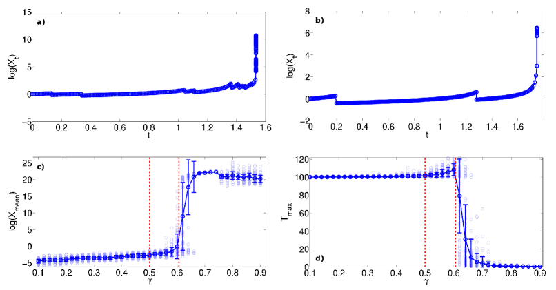
Figure 4: Results of simulations for SHS undergoing blowups; see text for more detailed description

6 Exact computations

We found the recurrence relations (31, 32) useful above in proving whether or not an SHS with certain parameters had blowups or not. In this section, we use recurrence relations to compute exact invariant distributions for SHS, for certain choices of $f$ and $\lambda$.

6.1 General relation

If we write $g(x)=\lambda(x)/f(x)$, and write $G^{\prime}(x)=g(x)$, then we compute:

$$S_{n} =\int_{0}^{T_{n+1}-T_{n}}\lambda(\varphi^{t}(X_{T_{n}}))\,dt$$

$$=\int_{0}^{T_{n+1}-T_{n}}g(\varphi^{t}(X_{T_{n}}))f(\varphi^{t}(X_{T_{n}}))\,dt$$

$$=\int_{0}^{T_{n+1}-T_{n}}g(\varphi^{t}(X_{T_{n}}))\frac{d}{dt}\varphi^{t}(X_{T_{n}})\,dt$$

$$=G(\varphi^{T_{n+1}-T_{n}}(X_{T_{n}}))-G(X_{T_{n}}).$$

Since $g(x)>0$ for all $x$, $G(x)$ is increasing, so we can write

$$X_{T_{n+1}}=\gamma\varphi^{T_{n+1}-T_{n}}(X_{T_{n}})=\gamma G^{-1}(S_{n}+G(X_{T_{n}})).$$

This identity holds true for any $f$, $\lambda$, but at the cost that $g(x)$ might be a rational function and thus $G(x)$ could be quite complicated. We get a nice solution if $g(x)$ is a monomial: if we assume that $g(x)=\delta x^{p}$,

$$(\varphi^{T_{n+1}-T_{n}}(X_{T_{n}}))^{p+1}-(X_{T_{n}})^{p+1} =(p+1)\delta^{-1}S_{n},$$

$$\gamma^{p+1}(\varphi^{T_{n+1}-T_{n}}(X_{T_{n}}))^{p+1} =\gamma^{p+1}((X_{T_{n}})^{p+1}+(p+1)\delta^{-1}S_{n}),$$

$$X_{T_{n+1}}^{p+1} =\gamma^{p+1}((X_{T_{n}})^{p+1}+(p+1)\delta^{-1}S_{n}).$$

Writing $Y_{n}=(X_{T_{n}})^{p+1}$, $\zeta=\gamma^{p}$, and $\theta=(p+1)/\delta$, gives the recursion

$$Y_{n+1}=(\zeta Y_{n}+\theta S_{n}).$$ (35)

Note that $\zeta\in(0,1)$, since it is a positive power of $\gamma$, and $\theta\in\mathbb{R}$. We compute

$$Y_{n}=\zeta^{n}Y_{0}+\theta\sum_{k=1}^{n}\zeta^{k}S_{k}.$$

Writing the final sum as

$$V_{n}=\theta\sum_{k=1}^{n}\zeta^{k}S_{k},$$

and assuming $X_{0}$ has finite moments of all orders, then for all $m>0$,

$$\lim_{n\to\infty}\mathbb{E}[(Y_{n})^{m}]=\mathbb{E}[(V_{n})^{m}],$$

and we can study the latter. Similarly, as $n\to\infty$, the pdf for $\zeta^{n}Y_{0}$ converges to $\delta(0)$, so

$$p_{Y_{n}}(z)=p_{\zeta^{n}Y_{0}+V_{n}}(z)=p_{\zeta^{n}Y_{0}}(z)*p_{V_{n}}(z)\to p_{V_{n}}(z),$$

and thus it is sufficient to study $V_{n}$ whether we are interested in particular moments, or a formula for its distribution. We now write down formulas for the moments and distribution of $V_{n}$.

6.2 Moments of $V_{n}$

Theorem 6.1.

The $m$th moment of $V_{n}$ is given by

$$\mathbb{E}[(V_{n})^{m}]=\theta^{m}\cdot m!\sum_{k=m}^{nm}\pi_{n}^{(k,m)}\zeta^{k},$$ (36)

where $\pi_{n}^{(k,m)}$ is the number of partitions of $k$ into $m$ positive parts, each of size less than or equal to $n$.

Proof.

Wlog assume $\theta=1$ by rescaling. We use the standard “generatingfunctionology” approach here: we write

$$\mathbb{E}[e^{tV_{n}}]=\mathbb{E}[e^{t\sum_{k=1}^{n}\zeta^{k}S_{k}}]=\mathbb{E}[\prod_{k=1}^{n}e^{t\zeta^{k}S_{k}}]=\prod_{k=1}^{n}\mathbb{E}[e^{t\zeta^{k}S_{k}}]=\prod_{k=1}^{n}\frac{1}{1-t\zeta^{k}},$$

where we have used independence of the $S_{k}$, and this formula is valid if $\left|{t}\right|<\zeta^{-k}$. We also have

$$\mathbb{E}[e^{tV_{n}}]=\mathbb{E}\left[\sum_{m=0}^{\infty}\frac{(tV_{n})^{m}}{m!}\right]=\sum_{m=0}^{\infty}\frac{t^{m}}{m!}\mathbb{E}[(V_{n})^{m}].$$

Thus the moment of interest is $m!$ times the coefficient of $t^{m}$ in the power series of $\mathbb{E}[e^{tV_{n}}]$.

We have

$$\prod_{k=1}^{n}\frac{1}{1-t\zeta^{k}} =\prod_{k=1}^{n}\sum_{\ell=0}^{\infty}(t\zeta^{k})^{\ell}=\sum_{\ell_{1},\ell_{2},\dots,\ell_{n}=0}^{\infty}\prod_{k=1}^{n}(t\zeta^{k})^{\ell_{k}}$$

$$=\sum_{\ell_{1},\ell_{2},\dots,\ell_{n}=0}^{\infty}t^{\sum_{k=1}^{n}\ell_{k}}\zeta^{\sum_{k=1}^{n}k\ell_{k}}$$

$$=\sum_{m=0}^{\infty}t^{m}\sum_{\begin{subarray}{c}\ell_{1},\ell_{2},\dots,\ell_{n}=0\\ \ell_{1}+\dots+\ell_{n}=m\end{subarray}}\zeta^{\sum_{k=1}^{n}k\ell_{k}}.$$

Therefore

$$\mathbb{E}[(V_{n})^{m}]=m!\sum_{\begin{subarray}{c}\ell_{1},\ell_{2},\dots,\ell_{n}=0\\ \ell_{1}+\dots+\ell_{n}=m\end{subarray}}\zeta^{\sum_{k=1}^{n}k\ell_{k}}$$

The coefficient of $\zeta^{k}$ in this sum is given by the number of integer solutions to the Diophantine system

$$\begin{split}\ell_{1}+\ell_{2}+\dots+\ell_{n}&=m,\\ \ell_{1}+2\ell_{2}+\dots+n\ell_{n}&=k.\end{split}$$ (37)

This number is equal to the number of partitions of $k$ into $m$ positive parts, each less than $n$. To see this, consider such a partition, ordered increasingly, so that it contains $\ell_{1}$ $1$’s, then $\ell_{2}$ 2’s, all up to $\ell_{n}$ $n$’s. Then by definition, the $\ell_{j}$ must satisfy (37). Conversely, any choice of $\ell_{j}$ satisfying (37) gives a partition in the obvious manner. This completes the proof. ∎

Corollary 6.2.

$$\mathbb{E}[(V_{\infty})^{m}]=\theta^{m}\cdot m!\sum_{k=m}^{\infty}\pi_{m}(k)\zeta^{k},$$

where $\pi_{m}(k)$ is the standard partition function of $k$ into $m$ positive parts [49].

Remark 6.3.

It is not entirely surprising that partition numbers appear in this computation. Again, let $\theta=1$ for simplicity. From Corollary 6.2 that the generating function of $V_{\infty}$ is the infinite product

$$\mathbb{E}[e^{tV_{\infty}}]=\prod_{\ell=1}^{\infty}\frac{1}{1-t\zeta^{\ell}}.$$

But we have

$$\mathbb{E}[e^{tV_{\infty}}]=\sum_{m=0}^{\infty}\frac{t^{m}}{m!}\mathbb{E}[(V_{\infty})^{m}]=\sum_{m=0}^{\infty}\sum_{k=m}^{\infty}\pi_{m}(k)t^{m}\zeta^{k}=\sum_{k=0}^{\infty}\zeta^{k}\sum_{m=0}^{k-1}t^{m}\pi_{m}(k).$$

Clearly $\sum_{m=0}^{k-1}\pi_{m}(k)$ is the standard partition function $\pi(k)$, and setting $t=1$ we obtain

$$\prod_{\ell=1}^{\infty}\frac{1}{1-\zeta^{\ell}}=\sum_{k=0}^{\infty}\zeta^{k}\pi(k),$$

recovering the well-known formula for the partition function.

6.3 Distribution of $V_{n}$

Theorem 6.4.

The probability distribution function of $V_{n}$ is given by

$$p_{n}(z)=\sum_{k=1}^{n}A_{k,n}(\zeta)e^{-z/\zeta^{k}}\mathbf{1}(z>0),$$

with

$$A_{k,n}(\zeta)=\frac{(-1)^{k-1}\zeta^{k(k-3)/2}}{\displaystyle\prod_{\begin{subarray}{c}j=1\\ j\neq k\end{subarray}}^{n}(1-\zeta^{\left|{j-k}\right|})}.$$

Proof.

We prove this by induction. Starting with $n=1$, we see that $A_{11}(\zeta)=1/\zeta$. Since $V_{1}=\zeta S_{1}$, and therefore

$$\mathbb{P}(V_{1}>z)=\mathbb{P}(\zeta S_{1}>z)=\mathbb{P}(S_{1}>z/\zeta)=e^{-z/\zeta}\mathbf{1}(z>0),\quad p_{1}(z)=-\frac{d}{dz}\mathbb{P}(V_{1}>z)=\frac{1}{\zeta}e^{-z/\zeta}\mathbf{1}(z>0).$$

This proves the formula for $p_{1}(z)$. Since $V_{n+1}=V_{n}+\zeta^{n+1}S_{n+1}$, we have

$$p_{n+1}(z) =\int_{-\infty}^{\infty}p_{n}(z-x)\zeta^{-(n+1)}e^{-x/\zeta^{n+1}}\mathbf{1}(x>0)\,dx$$

$$=\int_{-\infty}^{\infty}\sum_{k=1}^{n}A_{k,n}(\zeta)e^{-(z-x)/\zeta^{k}}\mathbf{1}(z-x>0)\zeta^{-(n+1)}e^{-x/\zeta^{n+1}}\mathbf{1}(x>0)\,dx$$

$$=\sum_{k=1}^{n}A_{k,n}(\zeta)e^{-z/\zeta^{k}}\int_{0}^{z}\zeta^{-(n+1)}\exp\left(\frac{\zeta^{n-k+1}-1}{\zeta^{n+1}}x\right)\,dx$$

$$=\sum_{k=1}^{n}A_{k,n}(\zeta)e^{-z/\zeta^{k}}\frac{1}{\zeta^{n-k+1}-1}\left(\exp\left(\frac{\zeta^{n-k+1}-1}{\zeta^{n+1}}z\right)-1\right)$$

$$=\sum_{k=1}^{n}A_{k,n}(\zeta)\frac{e^{-z/\zeta^{n+1}}-e^{-z/\zeta^{k}}}{\zeta^{n-k+1}-1}$$

$$=\sum_{k=1}^{n}\frac{A_{k,n}(\zeta)}{1-\zeta^{n-k+1}}e^{-z/\zeta^{k}}+e^{z/\zeta^{n+1}}\sum_{k=1}^{n}\frac{A_{k,n}(\zeta)}{\zeta^{n-k+1}-1}.$$

This gives us the recursion

$$A_{k,n+1}=\frac{A_{k,n}}{1-\zeta^{n-k+1}},\quad k<n+1;\quad A_{n+1,n+1}=\sum_{k=1}^{n}\frac{A_{k,n}}{\zeta^{n-k+1}-1}.$$

By plugging in, we see that the formula for $A_{k,n}$ satisfies the recursion relation, and we are done. ∎

Corollary 6.5.

The limit

$$A_{k}(\zeta):=\lim_{n\to\infty}A_{k,n}(\zeta)$$

exists for all $\zeta\in(0,1)$ (and in fact convergences uniformly), so that the distribution for $V_{\infty}$ is

$$p_{V_{\infty}}(z)=\sum_{k=1}^{\infty}A_{k}(\zeta)e^{-z/\zeta^{k}}.$$

Remark 6.6.

We have the following formulas for $A_{k}(\zeta)$:

$$A_{1}(\zeta)=\frac{1}{\zeta}\frac{1}{\prod_{k=1}^{\infty}(1-\zeta^{k})}=\frac{1}{\zeta}\sum_{k=1}^{\infty}\sum_{j=1}^{\infty}\zeta^{jk}=\frac{1}{\zeta}\sum_{n=1}^{\infty}\varphi(n)\zeta^{n},$$

where $\varphi(n)$ is the number of distinct factors of the integer $n$. For $k>1$, we have that

$$\frac{A_{k}(\zeta)}{A_{1}(\zeta)}=\frac{(-1)^{k-1}\zeta^{\frac{(k-2)(k-1)}{2}}}{\prod_{j=1}^{k-1}(1-\zeta^{j})}.$$

Moreover, for any fixed $\zeta\in(0,1)$,

$$\lim_{k\to\infty}A_{k}(\zeta)=0,$$

and in fact, for fixed $\zeta$ and $k$ sufficiently large,

$$\frac{A_{k}(\zeta)}{A_{k-1}(\zeta)}\approx\zeta^{k-2},$$

so that $A_{k}(\zeta)$ goes to zero superexponentially fast as $k\to\infty$.

7 Conclusions

We have presented many results for a class of SHS and examined the tension between instability arising from the flows and stability arising from the resets. The types of dynamical phenomena that we have observed share many features with both deterministic dynamical systems and stochastic processes.

One common feature of all of the systems studied here was that the state space was one-dimensional. Extending the types of results in this paper to higher dimensions could be challenging due to non-commutativity of flows.

8 Acknowledgments

This work was supported in part by the National Science Foundation (NSF) under awards ECCS-CAR-0954420, CMG-0934491, and CyberSEES-1442686, the Trustworthy Cyber Infrastructure for the Power Grid (TCIPG) under US Department of Energy Award DE-OE0000097, by the National Aeronautics and Space Administration through the NASA Astrobiology Institute under Cooperative Agreement No. NNA13AA91A issued through the Science Mission Directorate, and the Initiative for Mathematical Science and Engineering (IMSE) at the University of Illinois.

References

- [1] Richard Bellman. Limit theorems for non-commutative operations. I. Duke Mathematical Journal, 21(3):491–500, 09 1954.
- [2] M. H. A. Davis. Markov Models and Optimization. Chapman and Hall, London, UK, 1993.
- [3] Debasish Chatterjee and Daniel Liberzon. On stability of stochastic switched systems. Proceedings of the 43rd Conference on Decision and Control, 2004.
- [4] Debasish Chatterjee and Daniel Liberzon. Stability analysis and stabilization of randomly switched systems. In Decision and Control, 2006 45th IEEE Conference on, pages 2643–2648. IEEE, 2006.
- [5] G George Yin and Chao Zhu. Hybrid switching diffusions: properties and applications, volume 63. Springer, 2009.
- [6] João Pedro Hespanha and Abhyudai Singh. Stochastic Models for Chemically Reacting Systems Using Polynomial Stochastic Hybrid Systems. International Journal on Robust Control, Special Issue on Control at Small Scales: Issue 1, 15:669–689, September 2005.
- [7] João Pedro Hespanha. A Model for Stochastic Hybrid Systems with Application to Communication Networks. Nonlinear Analysis, Special Issue on Hybrid Systems, 62(8):1353–1383, September 2005.
- [8] J. P. Hespanha. Modelling and analysis of stochastic hybrid systems. IEE Proceedings–Control Theory and Applications, 153(5):520–535, September 2006.
- [9] Paul C Bressloff and Jay M Newby. Path integrals and large deviations in stochastic hybrid systems. Physical Review E, 89(4):042701, 2014.
- [10] Duarte Antunes, João Pedro Hespanha, and Carlos Silvestre. Stochastic hybrid systems with renewal transitions: Moment analysis with applications to networked control systems with delays. SIAM Journal of Control and Optimization, 51(2):1481–1499, February 2013.
- [11] S.V. Dhople, Y.C. Chen, L. DeVille, and A.D. Domínguez-García. Analysis of power system dynamics subject to stochastic power injections. IEEE Transactions on Circuits and Systems I: Regular Papers, 60(12):3341–3353, December 2013.
- [12] S. V. Dhople, L. DeVille, and A. D. Domínguez-García. A Stochastic Hybrid Systems framework for analysis of Markov reward models. Reliability Engineering & System Safety, 123:158–170, 2014.
- [13] Abhyudai Singh and João Pedro Hespanha. Approximate moment dynamics for chemically reacting systems. IEEE Transactions on Automatic Control, 56(2):414–418, February 2011.
- [14] Andrew R Teel, Anantharaman Subbaraman, and Antonino Sferlazza. Stability analysis for stochastic hybrid systems: A survey. Automatica, 2014.
- [15] Sean Meyn and Richard L. Tweedie. Markov Chains and Stochastic Stability. Cambridge University Press, New York, NY, USA, 2nd edition, 2009.
- [16] Yuri Bakhtin and Tobias Hurth. Invariant densities for dynamical systems with random switching. arXiv preprint arXiv:1203.5744, 2012.
- [17] Peter Milner, Colin S Gillespie, and Darren J Wilkinson. Moment closure approximations for stochastic kinetic models with rational rate laws. Mathematical biosciences, 231(2):99–104, June 2011.
- [18] Thilo Gross, Carlos J Dommar D’Lima, and Bernd Blasius. Epidemic dynamics on an adaptive network. Physical review letters, 96(20):208701, 2006.
- [19] Thilo Gross and IG Kevrekidis. Robust oscillations in SIS epidemics on adaptive networks: Coarse graining by automated moment closure. EPL (Europhysics Letters), page 6, February 2008.
- [20] Tim Rogers. Maximum-entropy moment-closure for stochastic systems on networks. Journal of Statistical Mechanics: Theory and …, page 20, March 2011.
- [21] JN Fry. The four-point function in the bbgky hierarchy. The Astrophysical Journal, 262:424–431, 1982.
- [22] M Keeling. Spatial models of interacting populations. Blackwell Science, Oxford, UK, 1999.
- [23] Matthew J Keeling. The effects of local spatial structure on epidemiological invasions. Proceedings of the Royal Society of London. Series B: Biological Sciences, 266(1421):859–867, 1999.
- [24] T J Newman, Jean-Baptiste Ferdy, and C Quince. Extinction times and moment closure in the stochastic logistic process. Theoretical population biology, 65(2):115–26, March 2004.
- [25] Robert R Wilkinson and Kieran J Sharkey. Message passing and moment closure for susceptible-infected-recovered epidemics on finite networks. Physical Review E, 89(2):022808, 2014.
- [26] Jared C Bronski and Richard M McLaughlin. The problem of moments and the majda model for scalar intermittency. Physics Letters A, 265(4):257–263, 2000.
- [27] James Colliander, Markus Keel, Gigiola Staffilani, Hideo Takaoka, and Terence Tao. Transfer of energy to high frequencies in the cubic defocusing nonlinear schrödinger equation. Inventiones mathematicae, 181(1):39–113, 2010.
- [28] Rafail Khasminskii. Stochastic stability of differential equations, volume 66. Springer, 2011.
- [29] Peter H Baxendale. Invariant measures for nonlinear stochastic differential equations. In Lyapunov Exponents, pages 123–140. Springer, 1991.
- [30] Peter H Baxendale. Stability and equilibrium properties of stochastic flows of diffeomorphisms. In Diffusion Processes and Related Problems in Analysis, Volume II, pages 3–35. Springer, 1992.
- [31] N. Sri Namachchivaya and H. J. Van Roessel. Moment Lyapunov Exponent and Stochastic Stability of Two Coupled Oscillators Driven by Real Noise. Journal of Applied Mechanics, 68(6):903, 2001.
- [32] J. R. Norris. Markov chains, volume 2 of Cambridge Series in Statistical and Probabilistic Mathematics. Cambridge University Press, Cambridge, 1998. Reprint of 1997 original.
- [33] Frigyes Riesz and Béla Sz.-Nagy. Functional analysis. Dover Books on Advanced Mathematics. Dover Publications, Inc., New York, 1990. Translated from the second French edition by Leo F. Boron, Reprint of the 1955 original.
- [34] Patrick Billingsley. Probability and measure. Wiley Series in Probability and Mathematical Statistics. John Wiley & Sons Inc., New York, third edition, 1995. A Wiley-Interscience Publication.
- [35] Jiangmeng Zhang, Lee DeVille, Sairaj V. Dhople, and Alejandro Domínguez-García. A maximum entropy approach to the moment closure problem for stochastic hybrid systems at equilibrium. In Proc. of the IEEE Control and Decision Conference, December 2014.
- [36] Mark Embree and LN Trefethen. Growth and decay of random Fibonacci sequences. Proceedings of the Royal Society A: Mathematical, Physical and Engineering Sciences …, 455:2471–2485, 1999.
- [37] SN Dorogovtsev, AV Goltsev, and JFF Mendes. Critical phenomena in complex networks. Reviews of Modern Physics, page 79, April 2008.
- [38] Nigel Goldenfeld. Lectures on phase transitions and the renormalization group. Addison-Wesley, Advanced Book Program, Reading, 1992.
- [39] H. Stanley. Scaling, universality, and renormalization: Three pillars of modern critical phenomena. Reviews of Modern Physics, 71(2):S358–S366, March 1999.
- [40] JP Sethna, KA Dahmen, and CR Myers. Crackling noise. Nature, 410(6825):242–50, March 2001.
- [41] Osame Kinouchi and Mauro Copelli. Optimal dynamical range of excitable networks at criticality. Nature Physics, 2(5):348–351, April 2006.
- [42] Thierry Mora and William Bialek. Are Biological Systems Poised at Criticality? Journal of Statistical Physics, 144(2):268–302, June 2011.
- [43] Daniel Larremore, Woodrow Shew, and Juan Restrepo. Predicting Criticality and Dynamic Range in Complex Networks: Effects of Topology. Physical Review Letters, 106(5):1–4, January 2011.
- [44] Nir Friedman, Shinya Ito, Braden AW Brinkman, Masanori Shimono, RE Lee DeVille, Karin A Dahmen, John M Beggs, and Thomas C Butler. Universal critical dynamics in high resolution neuronal avalanche data. Physical review letters, 108(20):208102, 2012.
- [45] Mark EJ Newman. Power laws, pareto distributions and zipf’s law. Contemporary physics, 46(5):323–351, 2005.
- [46] Aaron Clauset, Cosma Rohilla Shalizi, and Mark EJ Newman. Power-law distributions in empirical data. SIAM review, 51(4):661–703, 2009.
- [47] Adam Shwartz and Alan Weiss. Large deviations for performance analysis. Chapman & Hall, London, 1995.
- [48] Amir Dembo and Ofer Zeitouni. Large deviations techniques and applications, volume 38 of Stochastic Modelling and Applied Probability. Springer-Verlag, Berlin, 2010. Corrected reprint of the second (1998) edition.
- [49] The On-Line Encyclopedia of Integer Sequences. published electronically at http://oeis.org. Sequence A008284.