Characterizing the nonlinear interaction of S- and P-waves in a rock sample

Abstract

The nonlinear elastic response of rocks is known to be caused by the rocks’ microstructure, particularly cracks and fluids. This paper presents a method for characterizing the nonlinearity of rocks in a laboratory scale experiment with a unique configuration. This configuration has been designed to open up the possibility the nonlinear characterization of rocks as an imaging tool in a field scenario. The nonlinear interaction of two traveling waves: a low-amplitude 500 kHz P-wave probe and a high-amplitude 50 kHz S-wave pump has been studied on a room-dry 15 x 15x 3 cm slab of Berea sandstone. Changes in the arrival time of the P-wave probe as it passes through the perturbation created by the traveling S-wave pump were recorded. Waveforms were time gated to simulate a semi-infinite medium. The shear wave phase relative to the P-wave probe signal was varied with resultant changes in the P-wave probe arrival time of up to 100 ns, corresponding to a change in elastic properties of $0.2\%$. In order to estimate the strain in our sample, ae also measured the particle velocity at the sample surface to scale a finite difference linear elastic simulation to estimate the complex strain field in the sample, on the order of $10^{-6}$, induced by the S-wave pump. We derived a fourth order elastic model to relate the changes in elasticity to the pump strain components. We recover quadratic and cubic nonlinear parameters: $\tilde{\beta}=-872$, $\tilde{\delta}=-1.1\times 10^{10}$, respectively, at room-temperature and when particle motions of the pump and probe waves are aligned. Temperature fluctuations are correlated to changes in the recovered values of $\tilde{\beta}$ and $\tilde{\delta}$ and we find that the nonlinear parameter changes when the particle motions are orthogonal. No evidence of slow dynamics was seen in our measurements. The same experimental configuration, when applied to Lucite and aluminum, produced no measurable nonlinear effects. In summary, a method of selectively determining the local nonlinear characteristics of rock quantitatively has been demonstrated using traveling sound waves.

I Introduction

Mechanical waves provide information for characterizing the bulk properties of materials noninvasively. Classical methods usually create a map of linear information, such as elastic modulus, to detect structures. Imaging structures is just a beginning; many applications require more specific information with the goal of determining the quantitative nature of the structures. In rocks, nonlinear elastic properties vary over several orders of magnitude Belyayeva_1995 making them good candidates for imaging. This nonlinearity is primarily due to the microstructure of the rocks Guyer_1999 ; Guyer_2009 . An understanding of this microstructure is increasingly important for subsurface exploration. This study aims to characterize the nonlinearity of rocks in a laboratory scale experiment with a configuration that mimics a potential field scenario. In the experiment we perturb the propagation of a low amplitude high frequency P-wave probe with a high amplitude low frequency S-wave pump. We use a configuration with a large distance between the probe source and receiver (30 probe wavelengths) and a propagating pump wave. This experiment is designed as a preliminary study working toward an imaging method based on the nonlinear interaction of two waves.

Guyer et. al Guyer_1999 demonstrated that nonlinearities in rocks can be observed with strains as low as $10^{-8}$, this level of sensitivity means that almost any kind of wave propagation can induce a nonlinear effect; the challenge is in its detection. Field observation of nonlinear responses induced by strong or weak earthquakes are well documented (see Regnier_2013 for instance), and wave-speed variations on the order of 0.05% have been measured during earthquakes on the San Andreas fault Brenguier_2008 . Actively induced nonlinear responses have been observed in-situ at the scale of a few meters Kurtulus_2008 ; Johnson_2009 ; Lawrence_2009 ; Cox_2009 .

Laboratory measurements are also helpful in understanding the nonlinear elastic response. Of particular importance is the role of additional compliance due to micro-cracks including anisotropy and fluid saturation effects Holcomb_1981 ; Thomsen_1995 ; SAYERS_1995 ; Gueguen_2003 ; Fortin_2007 . These studies were based on changes in acoustic signals under quasi-static uni-axial stress or hydrostatic pressure. Because of the difficulty in measuring the small changes induced by nonlinearities at small strains ($10^{-8}-10^{-5}$), most laboratory studies of nonlinearity in rocks use samples in resonance JOHNSON_1991 ; TenCate_1996 ; Guyer_1999 ; Gusev_1998 ; DAngelo_2004 . At these strain amplitudes, no plastic deformation occurs and tiny perturbations of soft bonds are responsible for the nonlinear behavior Darling_2004 . These methods are generally based on monitoring the frequency and damping of particular resonances and thus they average the nonlinear response during several cycles of tension/compression.

To avoid this averaging, Dynamic Acousto-Elasticity (DAE) attempts to account for the dynamics of the nonlinear interaction within a cycle and is the closest method to the one proposed here. First developed in medical characterization of bone and other materials Renaud_2008 ; Renaud_2009 ; Muller_2006 , it was later applied to rocks Renaud_2012 ; Renaud_2013 ; Renaud_2013a ; Riviere_2013 . The method relies on monitoring the material several times during a resonant period. The monitoring is performed with a very low strain probe wave and the high strain resonant wave is called the pump. This probe wave monitors changes in the ultrasound properties, (wave-speed and attenuation), during the quasi-static compression and tension of the material, caused by the pump wave. This method takes advantage of a uniform strain along a short probe path due to both a 1-D geometry and the resonance of the sample. The ideas of DAE have also been applied for in-situ measurement by Renaud et al. Renaud_2013b .

With the goal of developing an imaging technique for the nonlinear elastic properties, we propose a DAE experiment with a unique configuration. First, the probe source-receiver distance is large compared to the pump wavelength. This allows us to estimate the nonlinearity not only locally around a source-receiver pair, but also in a larger region. Second, the resonant pump wave is replaced by a propagating wave, time-gated to mimic an infinite sample. We then measure the change in the arrival time of the probe as the pump wave crosses its path. Finally, the P-wave pump is replaced with an S-wave allowing us to change the relative particle motions of the pump and probe, by varying the polarization of the shear wave. In the following we detail the motivations for these three unique aspects of our experiment: large source-receiver distance, propagating pump and S-wave pump.

The possibility of nonlinear parameter tomography for a large source-receiver distance is treated theoretically for a harmonic field in Belyayeva et. al Belyayeva_1995 . Because we use a propagating wave in our experiment, the strain is neither uniform nor static along the probe path. The homogeneous strain distribution assumption also does not hold in Geza et al. Geza_2001 , where an attempt at nonlinear imaging is presented.

The propagating pump wave is common to all in-situ methods Kurtulus_2008 ; Johnson_2009 ; Lawrence_2009 ; Cox_2009 and has also been tested for a DAE method in Renaud_2013b . In these methods, the strain is generally estimated using embedded instruments. At the laboratory scale, a different option is preferred. Our sample mimics a 2D medium because the source wave transducer has a diameter approximately the same size as the smallest dimension of the sample. We can thus measure the strain on the surface and reasonably infer its distribution within the sample with finite difference modeling, resulting in an estimation of the strain distribution as a function of time. The pump wave field is different than it would be in a semi-infinite medium due to differences in geometrical spreading and conversions at the surface. However, the pump wave remains a propagating wave which is sufficient to illustrate the feasibility of the method for in-situ measurement. In addition, preliminary measurements in a cube show similar results

Both nonlinear propagation of seismic waves and in-situ methods of nonlinear characterization involve shear strain components, the interaction of which is the underlying physics of the nonlinear elasticity. There is a gap between field observations and laboratory experiments in rocks because, as far as the authors know, the nonlinear perturbation of the medium is usually considered to be due to only compressive strain components and does not typically include shear strain components. The reason for this may come from the absence of quadratic nonlinearity induced by a shear strain Belyayeva_1995 . Laboratory rock experiments include nonlinear effects on shear wave propagation such as shear wave splitting under uni-axial stress Toupin_1961 and shear wave generation from P-wave mixing Johnson_1989 , but this does not include a shear strain component in the origin of the nonlinearity. The choice of a shear wave pump in this paper aims to consider a realistic pump strain field in a subsurface experiment, that includes shear components. As for experiments, we found no theoretical studies on the effect of shear strain on nonlinear elasticity; to rectify this a fourth order elasticity model is presented, inspired by a series of papers by Destrade et. al Destrade_2010 ; Destrade_2010a ; Destrade_2010b .

The nonlinear characterization technique is presented in section II, by discussing the experimental set-up, signal acquisition procedure, and strain estimation method. A fourth order elasticity model is introduced in section II, followed by the definition of the nonlinear parameters measured experimentally. Experimental results are then presented in section IV to characterize the nonlinear response of a room-dry Berea Sandstone sample.

II Nonlinear wave mixing experiment

The characterization of nonlinearity requires two fundamental measurements. First the effect of the pump wave on the probe propagation is determined from the modulation of the propagation time through the sample. And second, the strain induced by the pump wave has to be measured in order to quantify the nonlinearity. This second step is done by the use of both a laser vibrometer to estimate the strain at the surface, and also numerical modeling of the pump propagation to estimate the strain in the whole sample.

II.1 Experimental set-up

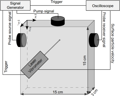
Figure 1: Experimental set-up: a P-wave transducer generates an ultrasonic pulse at 500 kHz in a $15\times 15\times 3$ cm sample. This probe signal is recorded, after propagation through the sample, by an identical transducer. The pump signal is generated with an S-wave transducer at 50 kHz. The particle velocity of the pump, polarized along the $x-$axis is measured with a laser vibrometer. The probe signal and particle velocity are digitized at 250 MHz by an oscilloscope triggered with the signal generator. The reference coordinate system has a $+x$ axis along the probe propagation (left to right), $+z$ axis pointing down and the $+y$ axis perpendicular to the large surface.

Figure 1 shows the experimental setup. We use a $15\times 15\times 3$ cm block of Berea Sandstone, with linear properties summarized in Table 1. We choose Berea Sandstone because it is relatively well-studied as well as relatively homogeneous. We generate the low-amplitude (strain less than $10^{-7}$, see section II.3) 500 kHz probe signal with a P-wave transducer with a 2.5 cm diameter (Olympus Panametrics Videoscan V102-RB) on the left face of the sample (i.e. propagating in the $+x-$direction); we record all signals with an identical P-wave transducer on the opposite face of the sample. The high-amplitude (strain around $10^{-6}$, see section II.3) S-wave pump ($F_{0}=50$ kHz) is transmitted from a S-wave transducer with a 2.5 cm diameter (Olympus Panametrics Videoscan V1548), placed on the top face of the sample (i.e. propagating in the positive $z-$direction with its particle motion aligned along the $+x$-axis in the $xz$-plane). The method for estimating the strain is described below; for the probe we had to amplify the signal so that it would be visible to the vibrometer, and then linearly scale the estimated strain back to the levels used in the original experiment. This gives us an order-of-magnitude estimate of the probe strain of $10^{-7}$ during the experiment. Even at these low strains, the probe wave is shown Riviere_2013 to have an effect on the nonlinear response, but this effect is limited to a slow dynamic effect (signals changing on the order of seconds to hours), which is independent of the pump period Johnson_2005 . Slow dynamic effects are not observed in this experiment as demonstrated in section IV.3. The higher amplitude S-wave pump does perturb the elastic properties of the medium, and it is these perturbations that we are interested in measuring via their nonlinear interaction with the P-wave probe. These interactions remain small, however, and so we compare the probe signal with and without the pump as described in section II.2. We record three signals for each data point. The probe alone ①, the pump and probe together ②, and then the pump alone ③. Each signal is independently averaged by the scope 16 times, before moving on to the next signal. Each signal is recorded for a duration of 20 $\mu$s. The entire sequence ①②③${}_{\phi_{0}}$ is recorded for a probe/pump delay $\phi=\phi_{0}$. Then the sequence is repeated for different delays: ①②③${}_{\phi_{0}}$,①②③${}_{\phi_{1}}$,①②③${}_{\phi_{2}}$… We vary the delay between the probe and pump signal over several periods of the pump to see the change in the probe traveltime as a function of the phase of the pump.

Compressional wave speed	$c_{p}=2450$ m/s
Shear wave speed	$c_{s}=1550$ m/s
Density	$\rho=2700$ kg/m³
Elastic modulus $\lambda+2\mu$	$M=16$ GPa
Length	$L=15\>\mathrm{cm}$
High	$H=15\>\mathrm{cm}$
Thickness	$e=3\>\mathrm{cm}$

Table 1: Berea Sandstone sample parameters

We excite the probe wave at a much lower frequency than the pump so that we can consider the pump wave to be in a steady-state during the probe propagation. For our experiment, the ratio of the excited P-wave probe wavelength to that of the S-wave pump is about 1/6, although the recorded difference is somewhat smaller (see Figure 2), due to dispersion in the sample. The choice of a shear wave for the pump allows us to control the main direction of strain and gives a slower change in the strain distribution. The number of cycles of the pump signal is chosen to avoid reflections from the bottom of the sample ($z=15$ cm) in order to mimic a semi-infinite medium with no resonance. The wavelength at this frequency is $\lambda_{s}=3.1$ cm so, with 6 cycles, and a return-time of 200 $\mu$s, there is no reflection returning within the time of the probe propagation across the sample (60 $\mu$s). The maximum delay of the probe excitation (after the pump excitation) is $\phi=120~{}\mu$s. After probe excitation, the total observation time (180 $\mu$s) is still less than the return time. The probe wavelength ($\lambda_{p}=4.5$ mm) ensures that the perturbation induced by the shear wave pump is uniform as seen by the probe propagation. The phase delay between the probe and the pump signals is changed to scan several cycles of tension and compression induced by the pump.

We use an arbitrary waveform generator to create the probe, pump and trigger signals. A power amplifier is needed for the pump signal in order to reach sufficiently high strains. At the receiving P-wave transducer, we are interested in the probe signal and not in the pump; obviously when the pump and probe are both active, we record both signals. To mitigate this, a second order high-pass frequency filter, with a cut-off frequency $f_{c}=150$ kHz, is used to minimize the amplitude of the pump signal measured at the receiver, so that mainly the probe signal is recorded. The attenuation of the filtering is compensated with a pre-amplifier (+50 dB). In addition, we use a low-pass filter, cut-off frequency $f_{c}=1.5$ MHz to eliminate some high-frequency noise. The acquisition of the probe signal by the P-wave receiver and the shear pump displacement measured by the laser vibrometer are synchronized via the trigger signal. The electronics are fully controlled via MATLAB: transmission and receiving parameters, as well as the recording of the signals. The delay $d_{p}=8$ ms between two consecutive acquisitions, for example between ① and ② is chosen to avoid the superposition of consecutive signals, i.e. to avoid recording the reverberation of the shear wave pump in the sample. For the same reason the delay is the same between two consecutive sequences ①②③${}_{\phi_{0}}$ and ①②③${}_{\phi_{1}}$.

II.2 Nonlinear signal observation

Each data point is obtained from the three signals shown in Figure 2. First, we record ① the probe pulse with no pump present, shown in a). Second, we record ② the perturbed probe with the pump turned on: solid line in b). Third, we record ③ the pump signal alone (dashed line, b). We then subtract the pump signal (dashed) from the perturbed probe and pump signal (solid) to estimate the perturbed probe, shown in c). The perturbed probe, Figure 2 c), is compared to the original one to estimate the nonlinear perturbation.

The measured arrival time modulation $TM_{meas}$, induced by the interaction over the propagation path of the probe wave with the pump wave, is defined as

$$TM_{meas}\left(\phi\right) = T_{p}\left(\phi\right)-T_{o}\left(\phi\right),$$ (1)

where $T_{o}$ is the arrival time of the original probe, $T_{p}$ that of the perturbed probe, and $\phi$ is the phase shift (a time delay added to the transmitted pulse) between the probe and pump signals. $TM$ is measured by cross-correlating the original (shown in Figure 2a)) and the perturbed (shown in Figure 2c)) pulses. The correlation is computed in a two period window, centered on the maximum of the signal ($3.3\,\mu s<t<7.3\,\mu s$ in Figure 2). The changes in travel time are small, much smaller than the time sampling interval, so we interpolate the peak of the cross-correlation with a second-order polynomial before picking the maximum Catheline_1999 . We discard data for which the waveforms change, defined as a correlation coefficient of less than 0.99. We observed that the subtraction of the low frequency part of the signal does not modify the waveform, and that the perturbation is small enough to neglect any stretching of the probe pulse due to distortion of the waveform.

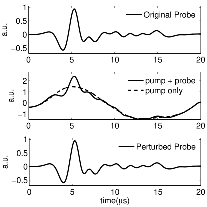
Figure 2: a) First, the original response to the probe pulse with no perturbation (① solid line) is recorded on the receiver. b) Next, we turn on the shear wave pump to record the superposition of the pump and probe signals (② solid line). Finally, the response to the pump with no probe is also recorded (③ dashed line). c) The perturbed probe, constructed from the difference between solid and dashed line in b), is compared to the original probe at each phase. In this example the phase shift between pump and probe is $\phi=25~{}\mu s$. Note that at 50 kHz, the pump signal is attenuated by -54 dB with a high-pass filter. “Arbitrary units” is abbreviated as “a.u.”

The $TM_{meas}$ between the original and perturbed probe is shown as a function of the phase shift between the probe and pump in Figure 3, solid line). Each point is an average of 30 acquisitions. We apply a low pass filter with a cutoff frequency at 100 kHz (twice the pump frequency) to $TM_{meas}(\phi)$ to remove high frequency components induced by noise. The signal $TM_{meas}(\phi)$ clearly has two frequency components, one around the pump frequency as well as a very low frequency trend. The presence of the pump frequency suggests that $TM_{meas}$ contains a term proportional to the pump strain, this is the so-called quadratic nonlinearity. Then, the low frequency trend requires an additional term that is always positive. The most likely candidate is the square of the strain; this cubic linearity is known to be large in rocksGuyer_1999 . Because the probe wave experiences approximately three tension-compression cycles during its propagation from source to receiver, the hysteresis known to play an important role rocks (Holcomb_1981 ) can not be clearly observed.

We repeated the experiment in aluminum and lucite, as shown in Figure 3 the measured time modulation is very small in these materials ($\pm 0.2$ ns), without any clear component at the pump frequency. These signals are at least an order of magnitude higher than what we would expect for aluminum ($TM\approx 0.5$ ns for a $10^{-5}$ strain according to Renaud_2012 ; our strain is $\sim 10^{-6}$) and are almost certainly experimental noise. In Lucite, the nonlinear parameters are even smaller (see Winkler_1996 ), confirming the significance of both aluminum and Lucite measurements. This comparison with standard linear material ensures that $TM_{meas}$ does not originate in the lab equipment, but depends on the sample studied.

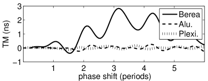
Figure 3: A comparison of the nonlinear response of different materials. The responses in both Lucite and Aluminum shown as dashed and dotted lines are significantly smaller than those recorded for Berea Sandstone as a solid line.

II.3 Estimating the strain

As will be shown in the following section, the characterization of the nonlinearity directly relies on the estimation of the strain pump. We thus need to characterize the pump field within the sample. At the order of magnitude ($<10^{-5}$ in strain) and at the pump frequency (50 kHz) we are considering, direct measurements are impossible to perform with strain gauges. Previous studies used a laser vibrometer to measure the particle velocity at a particular point on the sample, and then interpolated the strain assuming vibration at a single resonance Renaud_2012 . A similar method is used in this experiment, but since the wave-field is not a single resonance, we require a more careful numerical modeling of the wavefield.

II.3.1 Numerical model

We use a 3D, isotropic, purely-elastic (i.e. lossless) finite difference model, following the method described in references Virieux_1986 ; Graves_1996 , to model the linear propagation of the shear wave pump. We apply free-surface boundary conditions on all sides of the sample, and compute the stress and particle velocities on a staggered grid. The same geometry and wave speeds mentioned in section II.1 are used as input parameters to the model; the geometry is shown in figure 1. The spatial meshing of the model is 0.5 mm and the time sampling is 0.08 $\mu$s.

The challenge in modeling this experiment is in obtaining an accurate model of the transducer, so that the modeled and recorded waveforms match one another. We model the transducer with 1250 point force sources distributed on a disk with a diameter of 2.5 cm. We then use the x-component of the particle velocity ($V_{x}$) recorded by a laser vibrometer (polytech CLV-3D, see Fig. 1) as the input force signal for the simulation. In other words, we record the particle velocity experimentally, and then use that signal to drive the simulated transducer. Note that the laser signal records the surface particle velocity at the position ($x=7.5,\>y=3,\>z=3.6$ cm) while the shear transducer creates a force along the $x-$axis at the position ($x=7.5,\>y=1.5,\>z=0$ cm). Because of this, we scale the amplitude of the numerical result to match that of the experiment. This is valid because we are doing a linear simulation. The scaling of the model using only a single point measurement of particle velocity may induce errors in the strain estimation, particularly when there are diffraction effects.

II.3.2 Pump strain field

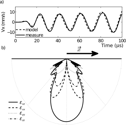
Figure 4: a) The x-component of the particle velocity at ($x=7.5,\>y=3,\>z=3.6$ cm) is measured with a laser vibrometer (solid line) and modeled with a finite difference simulation (dashed line). b) Polar radiation patterns of the shear transducer are shown for the shear strain $\epsilon_{xz}$ (solid line), and the compressive strains $\epsilon_{xx}$ (dashed line), $\epsilon_{yy}$ (dotted line), and $\epsilon_{zz}$ (dash-dotted line). The arrow represents the transducer force direction ($x-$axis).

Figure 4 a) shows good first order agreement between $V_{x}$ measured by the laser and modeled, after calibration. The apparent small difference in frequency between the two signals could be caused by a number of things, the most likely of which is interferences of different wave types. From the calibrated simulation, we obtain the stress throughout the sample, at all times. We then compute the strain, using a linear Hooke’s law.

The elastic response of the sample does not contain a pure shear wave since the transducer has a finite size. The radiation pattern of the transducer is represented in polar coordinates in Figure 4 b) for different strain components. The radiation pattern represents the relative amplitude of each strain as a function of the angle in the $xz$-plane for a strain $\epsilon_{ij}$ and at a 3-cm distance from the transducer. The main strain component is the shear $\epsilon_{xz}$ strain that corresponds to the propagating S-wave pump. The strain magnitudes can be compared by computing the absolute maxima of each strain ($\|\epsilon_{ij}\|$). The following ratios are found :

$$\|\epsilon_{xz}\|\approx 1.5\|\epsilon_{xx}\|\approx 2\|\epsilon_{zz}\|\approx 3\|\epsilon_{yy}\|\approx 20\|\epsilon_{xy}\|\approx 40\|\epsilon_{yz}\|.$$ (2)

The compressive strains are on the same order of magnitude but the shear strain $\epsilon_{xy}$ and $\epsilon_{yz}$ can be neglected and thus are not represented in Figure 4. The components $\epsilon_{xz}$ and $\epsilon_{xx}$ have a similar pattern to that of the tangential and radial component of the displacement field created by a shear transducer in an elastic half-space. The other two components $\epsilon_{yy}$ and $\epsilon_{zz}$ are not present in a half-space but arise from the limited size of the sample along the $y-$direction and thus need to be taken into account in the nonlinear characterization of the material.

II.3.3 Probe strain field

For the probe strain estimation we apply a similar method with a few changes. First, another laser vibrometer was utilized to achieve a higher sensitivity around the probe frequency 500kHz (a Polytech system with a OFV-505 optics head controlled by OFV-5000 with VD-06 decoder). Second, a sufficient amplitude of excitation was used to obtain a signal significantly above the noise. The particle velocity was deduced by increasing the input amplitude and then scaling the laser-measured amplitude. The input maximum voltage for the probe source transducer was set at 10 times the usual voltage: 20 V instead of 2 V. With a 2-V input signal, only the transducer was sensitive enough to measure a signal; the laser vibrometer signal was too noisy to obtain a reliable signal. The linearity of the transducer emission was checked by comparing the acoustic signal recorded by the probe receiver (Figure 1) with a 2-V and a 20-V input. Both signals have the same waveform and vary by a factor 10 in amplitude. We measured the resulting $x-$component of the particle velocity close to the probe receiver at ($x=15,\>y=1.5,\>z=1$ cm). We then divide the particle velocity by a factor 10 to scale the amplitude of the numerically modeled strain data. In addition to this scaling, the positions and the directions of the point force sources were changed for the probe simulation (see Figure 1). The result shows that the volumetric strain decreases nearly linearly along the propagation path from $9\times 10^{-8}$ around $x=0$ cm to $4\times 10^{-8}$ around $x=15$ cm. The value of $10^{-7}$ used above can thus be thought of as a rough upper bound for the strain excited by the probe.

III Theoretical description of the nonlinearity

In this section we establish a fourth order nonlinear Hooke’s law that relates the pump strain to the elasticity variation. This model depends on many elastic moduli that can not all be measured in the present experiment. We then present an approximation of the model and two nonlinear coefficients are defined. Finally we relate the measured change in travel-time to the nonlinear coefficients.

III.1 Fourth order elasticity theory

As mentioned in section II.2, the present experiment requires a model of the elastic response which includes both quadratic and cubic nonlinearities. In addition, the probe wave interacts with the pump wave over several cycles and we observe no hysteresis. Consequently, hysteresis is not included in the model. The description of a nonlinear elastic system starts from the strain energy $W$. The stress $\sigma_{ij}$ associated with the strain is then given by

$$\sigma_{ij}=\frac{\partial W}{\partial\epsilon_{ij}}\,,$$ (3)

where $\epsilon_{ij}=\frac{\partial u_{i}}{\partial x_{j}}$ is the Eulerian strain with $u_{i}$ the displacement along the $i$-axis with $i=x,y,z$. The derivative in Eq. 3 implies that the strain energy must be fourth-order in the strain to result in a third order (cubic) stress-strain relationship. For an isotropic material (we neglect the4% anisotropy measured in our sample) Landau and Lifshitz Landau_1986 show that the strain energy can be described by the three invariants:

$$I_{k}=tr(L^{k}),\qquad k=1,2,3$$ (4)

where $L$ is the Lagrangian strain : $L_{ij}=\frac{1}{2}(\epsilon_{ij}+\epsilon_{ji}+\sum_{k}\epsilon_{ki}\epsilon_{kj})$. The subscript denotes the minimum order of the invariant $I_{1,2,3}$; these invariants are the traces of $L$, $L^{2}$, $L^{3}$, respectively. For linear elasticity only the first two orders are considered: $I_{1}$ and $I_{2}$. Landau & Lifshitz Landau_1986 write the strain energy $W_{3}$ up to third order by including terms in $I_{3}$, $I_{1}I_{2}$ and $I_{1}^{3}$. There are 4 combinations of the invariants in the strain energy at the fourth order: $I_{1}I_{3}$, $I_{1}^{2}I_{2}$, $I_{2}^{2}$ and $I_{1}^{4}$, thus the fourth-order strain energy is Zabolotskaya_1986 ; Jacob_2007 ; Destrade_2010b ; Abiza_2012 :

$$W=\frac{\lambda}{2}I_{1}^{2}+\mu I_{2}+\frac{A}{3}I_{3}+BI_{1}I_{2}+\frac{C}{3}I{}_{1}^{3}+EI_{1}I_{3}+FI_{1}^{2}I_{2}+GI_{2}^{2}+HI{}_{1}^{4}\,,$$ (5)

where $A$, $B$ and $C$ are the third order elastic moduli introduced by Landau-Lifshitz Landau_1986 , and $E,\;F,\;G$ and $H$ are the fourth order elastic moduli Zabolotskaya_1986 .

In order to understand the present experiment, we first consider the ideal case of a P-wave probe propagating along the $x-$axis and a pure S-wave pump propagating along $z-$axis polarized along the $x-$axis. The probe and pump waves induce $\epsilon_{xx}$ and $\epsilon_{xz}$ strain components, respectively. The strain energy $W$, computed as a function of these two strain components including terms at the fourth order and below is

$$W=\frac{M}{2}\epsilon_{xx}^{2}+\frac{\mu}{2}\epsilon_{xz}^{2}+\gamma_{1}\epsilon_{xx}^{3}+\gamma_{2}\epsilon_{xx}\epsilon_{xz}^{2}+\gamma_{3}\epsilon_{xx}^{4}+\gamma_{4}\epsilon_{xx}^{2}\epsilon_{xz}^{2}+\gamma_{5}\epsilon_{xz}^{4}\,.$$ (6)

In Eq. 6, the linear elastic modulus, $M$ is given by

$$M=\lambda+2\mu\,,$$

the third order coefficients are

$$\gamma_{1}=\frac{M}{2}+\frac{A+3B+C}{3}\,,$$

$$\gamma_{2}=\frac{M}{2}+\frac{A+2B}{4}\,,$$

and the fourth order coefficients are

$$\gamma_{3}=\frac{M}{8}+\frac{A+3B+C}{2}+E+F+G+H\,,$$

$$\gamma_{4}=\frac{M}{4}+\frac{5A+14B+4C}{8}+\frac{3E+2F+4G}{4}\,,$$

and

$$\gamma_{5}=\frac{M}{8}+\frac{A+2B}{8}+\frac{G}{4}\,.$$

The stress is computed from the strain energy by $\sigma_{ij}=\frac{\partial W}{\partial\epsilon_{ij}}$; because we are interested in changes in the probe wave, we require only $\sigma_{xx}$, the probe stress

$$\sigma_{xx}=M\epsilon_{xx}+3\gamma_{1}\epsilon_{xx}^{2}+\gamma_{2}\epsilon_{xz}^{2}+4\gamma_{3}\epsilon_{xx}^{3}+2\gamma_{4}\epsilon_{xx}\epsilon_{xz}^{2}\,.$$ (7)

In Eq. 7, the first term (Hooke’s law) is responsible for linear probe wave propagation, the second and fourth terms are the quadratic and cubic nonlinearities in the probe propagation respectively, and the third term governs the nonlinear propagation of the pump. It is the fifth term $2\gamma_{4}\epsilon_{xx}\epsilon_{xz}^{2}$ that describes the interaction of the two waves. Renaming the probe strain $\epsilon_{p}=\epsilon_{xx}$ to highlight the amplitude difference between probe and pump: $\epsilon_{p}\ll\epsilon_{xz}$, we observe that this interaction term is clearly the dominant nonlinear effect. We then simplify Eq. 7 to include only the linear propagation and the interaction of the pump and probe

$$\sigma_{xx}=\epsilon_{p}\left(M+2\gamma_{4}\epsilon_{xz}^{2}\right)\,.$$ (8)

From Eq. 8, the importance of the cubic term in $\epsilon_{p}\epsilon_{xz}^{2}$ for the nonlinear coupling is highlighted. In this case there is no quadratic coupling term in ($\epsilon_{p}\epsilon_{xz}$) because the corresponding term in strain energy ($\epsilon_{p}^{2}\epsilon_{xz}$) is not present. Other pump strain components will introduce this dependence. Including this stress in the dynamic response of the elastic system gives a nonlinear (wave-like) equation of propagation for the P-wave probe

$$\rho\ddot{u}_{x}=\frac{\partial\sigma_{xx}}{\partial x}=\frac{\partial^{2}u_{x}}{\partial x^{2}}M\left(1+\frac{\mathrm{d}M}{M}\right)\,.$$ (9)

In section III.3, we show that the nonlinear term $dM/M$ is directly related to the measured arrival time modulation. In the simplified example discussed here, $dM/M$ contains only a cubic term: $dM/M=\delta_{xz}\epsilon_{p}\epsilon_{xz}^{2}$, with $\delta_{xz}=2\gamma_{4}$ the cubic coefficient reported in line 3 of Table 2.

pump strain ($\epsilon_{ij}$) quadratic coefficient ($\beta_{ij}$) cubic coefficient($\delta_{ij}$) $\epsilon_{xx}$ $3+2(A+3B+C)/M$ $3/2+6\left(A+3B+C\right)/M+12\left(E+F+G+H\right)/M$ $\epsilon_{yy},\>\epsilon_{zz}$ $\lambda/M+2(B+C)/M$ $\lambda/2M+2\left(B+C\right)/M+4\left(F+G+3H\right)/M$ $\epsilon_{xz},\,\epsilon_{zx},\,\epsilon_{xy},\,\epsilon_{yx}$ $0$ $1/2+\left(5A+14B+4C\right)/4M+\left(3E+2F+4G\right)/2M$ $\epsilon_{yz},\>\epsilon_{zy}$ $0$ $\lambda/2M+\left(3B+2C\right)/2M+\left(F+2G\right)/M$

Table 2: Fourth order nonlinear coupling between a P-wave inducing a compressive strain along the $x-$axis $\epsilon_{p}$ and all possible pump strain components. In the stress-strain relationship, the quadratic coefficient $\beta_{ij}$ weights the term in $\epsilon_{p}\epsilon_{ij}$, and the cubic one $\delta_{ij}$ the term in $\epsilon_{p}\epsilon_{ij}^{2}$. On the first line, $\epsilon_{xx}$ is the pump strain and do not includes the probe strain $\epsilon_{p}$.

This ideal case of a pure shear wave illustrates the computation of the fourth order wave mixing coefficients, but in Section II.3 we note that the pump wave field is more complex than a pure shear strain. We thus need to consider other strain components. For a P-wave probe propagating along the $x-$axis, there are 4 combinations of pump strain summarized in Table 2. For each case the strain energy is computed and the nonlinear stress-strain relationship is obtained by differentiating $W$ with respect to $\epsilon_{xx}$ (as in Eqs. 6 to 8). The linear term remains unchanged since it relates to the linear propagation of the probe and not to nonlinear wave mixing. Each combination of strain gives one quadratic coefficient, which weights the coupling between the probe strain $\epsilon_{p}$ and the pump strain $\epsilon_{ij}$, and one cubic coefficient for the coupling with $\epsilon_{ij}^{2}$. In the case of a P-wave pump along the $x-$axis, $\epsilon_{xx}$ includes both the probe strain $\epsilon_{p}$ and the pump strain $\epsilon_{xx}$ . Substituting $\epsilon_{xx}\equiv\epsilon_{p}+\epsilon_{xx}$ along with $\epsilon_{xz}=0$ in Eq. 7 and neglecting the nonlinear propagation of waves ($\epsilon_{p}^{2}$, $\epsilon_{p}^{3}$, $\epsilon_{xx}^{2}$ and $\epsilon_{xx}^{3}$) yields the probe stress $\sigma_{xx}$

$$\sigma_{xx}=M\epsilon_{p}+6\gamma_{1}\epsilon_{p}\epsilon_{xx}+12\gamma_{3}\epsilon_{p}\epsilon_{xx}^{2}\,.$$ (10)

The quadratic coefficient $\beta_{xx}=6\gamma_{1}/M$ and the cubic coefficient $\delta_{xx}=12\gamma_{3}/M$ are reported in the first line of Table 2. The quadratic coefficients gathered in Table 2 (second column) were obtained by Guyer et. al (Guyer_2009, , p. 47) and the cubic coefficients are given in (Hamilton_1998, , p.268) as a function of the elastic tensors ($C_{ijk}$ and $C_{ijkl}$). The quadratic coefficient is nonzero only with a compressive strain pump, this is confirmed in (Hamilton_1998, , p. 266) where the third order elastic tensor $M_{ijklmn}$ is found to be zero for a shear strain pump ($i=j=k=l$, and $m\neq n$).

III.2 Nonlinear coefficients approximation

From the strain pump characterization, in Section II.3, we know that $\epsilon_{xx},\>\epsilon_{yy},\>\epsilon_{zz}$ and $\epsilon_{xz}$ are of the same order of magnitude; the other strain components are at least an order of magnitude smaller and can thus be neglected. Consequently a complete expression of the fourth-order nonlinear elastic model of our experiment is given by

$$\frac{\mathrm{d}M}{M}=\beta_{xx}\epsilon_{xx}+\beta_{yy}\epsilon_{yy}+\beta_{zz}\epsilon_{zz}+\delta_{xx}\epsilon_{xx}^{2}+\delta_{yy}\epsilon_{yy}^{2}+\delta_{zz}\epsilon_{zz}^{2}+\delta_{xz}\epsilon_{xz}^{2}\,.$$ (11)

This expression contains seven interconnected parameters, which include all of the seven fourth-order elastic parameters. The experiment does not allow us to estimate all parameters independently, we thus need to simplify Eq. 11. First of all, the order of magnitude for linear, quadratic, and cubic elastic moduli are different (i.e. $\lambda,\>\mu<<A,\>B,\>C<<E,\>F,\>G,\>H$) and we can thus neglect terms containing linear moduli in the expressions for the quadratic moduli, and terms with the linear and quadratic moduli in the expression for the cubic moduli. Since only the quadratic and cubic nonlinearities can be measured independently in our experiment, we need to go from 7 unknowns to only 2. One simple way to achieve this is to assume that quadratic coefficients are of the same order of magnitude: $A\approx B\approx C$, and the same assumption for the cubic coefficients: $E\approx F\approx G\approx H$. This lead to a proportionality between the different coefficients of the same order: $\frac{\beta_{xx}}{10}\approx\frac{\beta_{yy}}{4}\approx\frac{\beta_{zz}}{4}$ and $\frac{\delta_{xx}}{48}\approx\frac{\delta_{yy}}{20}\approx\frac{\delta_{zz}}{20}\approx\frac{2\delta_{xz}}{9}$. Under these assumptions, the approximate nonlinearity is:

$$\frac{\mathrm{d}M}{M} \approx\tilde{\beta}\left(\epsilon_{xx}+\frac{2}{5}\epsilon_{yy}+\frac{2}{5}\epsilon_{zz}\right)$$

$$+\tilde{\delta}\left(\epsilon_{xx}^{2}+\frac{5}{12}\epsilon_{yy}^{2}+\frac{5}{12}\epsilon_{zz}^{2}+\frac{3}{32}\epsilon_{xz}^{2}\right)\,.$$ (12)

The nonlinear parameters $\tilde{\beta}$ and $\tilde{\delta}$ are coefficients of the quadratic and cubic nonlinearity respectively and can be thought of as averaged elastic moduli : $\tilde{\beta}\equiv\frac{\left(A+B+C\right)}{3M}$, $\tilde{\delta}\equiv\frac{\left(E+F+G+H\right)}{4M}$. They are representative of the nonlinearity but can vary with the strain distribution since the approximation implies that all strain invariants of the same order play the same role in the strain energy (Eq. 5). Those parameters can also be considered as empirically defined since only one parameter per order of nonlinearity can be measured with one configuration of probe and pump waves.

Such a model is useful for describing the elastic response of the rock at a fixed pump amplitude. Nevertheless, it does not capture all the complexity of the mechanical response of the rock because the nonlinear coefficients change with the pump amplitude as will be shown in section IV.5. The nonlinear characterization of rocks depends on the amplitude of the perturbation, this is why the quantification of the strain is so important. This also implies that monitoring or imaging nonlinearities has to be done with a constant pump amplitude to ensure repeatability.

III.3 Relating measurements to the nonlinear parameters

In a linear elastic medium the wave speed $c_{p}$ is constant or equivalently the stress $\sigma$ is proportional to the strain $\epsilon$ as in Hooke’s law: $\sigma=\epsilon M$, with the elastic modulus $M=\lambda+2\mu$, where $\lambda$ and $\mu$ are the Lamé parameters. A consequence of Hooke’s law is a constant wave speed $c_{p}^{2}=M\rho^{-1}$, with $\rho$ the density of the material. In this section, we detail the necessary extension of Hooke’s law for the nonlinear wave mixing considered in this experiment. The arrival time modulation induced by the pump strain (Fig. 3), can be explained as a variation of the wave speed $c_{p}$, or equivalently the elastic modulus $M$. Assuming a homogeneous medium, $c_{p}$ can also be defined as $c_{p}=\ell_{x}T^{-1}$ where $T$ is the time of propagation along a distance $\ell_{x}$ (assumed to be along the $+x$-axis). Differentiating both expressions for $c_{p}$ gives

$$\frac{\mathrm{d}c_{p}}{c_{p}}=\frac{\mathrm{d}\ell_{x}}{\ell_{x}}-\frac{\mathrm{d}T}{T},$$ (13)

and

$$\frac{\mathrm{d}c_{p}}{c_{p}}=\frac{\mathrm{d}M}{2M}-\frac{\mathrm{d}\rho}{2\rho}\,.$$ (14)

In rocks, the variation in distance of propagation $\mathrm{d}\ell_{x}$ and density $\mathrm{d}\rho$ can be neglected Renaud_2011 in Eq. 13 and 14 respectively. Equating these two expressions shows that changes in time and elastic modulus are proportional to one another, i.e. that

$$\frac{\mathrm{d}T}{T}=-\frac{\mathrm{d}M}{2M}\,.$$

For an infinitesimal distance along the propagation path $dl$, the propagation time is $T=dl/c_{p}$, the change in arrival time is then

$$\mathrm{d}T\approx-\frac{dl}{2c_{p}}\frac{\mathrm{d}M}{M}\,.$$ (15)

To go from the infinitesimal changes in time and modulus to the observed changes in travel time, we need to integrate equation 15 over the path length $\Gamma$

$$TM_{NL}=-\frac{1}{2c_{p}}\int_{\Gamma}\frac{\mathrm{d}M}{M}\,dl\,.$$ (16)

In equation 16, $TM_{NL}$ models the arrival time modulation measured in Figure 3 as a function of the variation of the elastic nonlinearity $dM/M$, integrated over the propagation path. In addition, the nonlinearity is a function of the pump strain as defined in Eq. 12. To estimate $TM_{NL}$ from the pump strain as described in section II.3, and because the pump transducer is approximately the same size as the S-wave pump wavelength, the strain needs to be averaged within the ultrasonic beam. For the sake of clarity, this average is included in the strain notation: $\epsilon_{ij}\left(l,T\right)\equiv<\epsilon_{ij}\left(l,r,T)\right>_{r}$, where $r$ is the radius of the beam. With this, along with the insertion of $T=l/c_{p}$ into the time variable of the strain, the time modulation from the nonlinear elasticity $TM_{NL}$ along the whole propagation path becomes

$$TM_{NL}\left(\phi\right)=- \frac{\tilde{\beta}}{2c_{p}}\int_{\Gamma}\epsilon\left(l,\phi+\frac{l}{c_{p}}\right)dl$$

$$-\frac{\tilde{\delta}}{2c_{p}}\int_{\Gamma}\epsilon^{2}\left(l,\phi+\frac{l}{c_{p}}\right)dl\,,$$ (17)

where $\epsilon=\epsilon_{xx}+\frac{2}{5}\epsilon_{yy}+\frac{2}{5}\epsilon_{zz}$ and $\epsilon^{2}=\epsilon_{xx}^{2}+\frac{5}{12}\epsilon_{yy}^{2}+\frac{5}{12}\epsilon_{zz}^{2}+\frac{3}{32}\epsilon_{xz}^{2}$, these strains includes the average within the ultrasonic beam. In the present experiment, with a homogeneous material, the propagation path $\Gamma$ is a straight line of length $L$ along the $x-$axis. In this case, the total arrival time modulation can be written as

$$TM_{NL}\left(\phi\right)=\tilde{\beta}\>Q\left(\phi\right)+\tilde{\delta}\>C\left(\phi\right)\,,$$ (18)

where the quadratic term is defined as:

$$Q\left(\phi\right)=-\frac{1}{2c_{p}}\int_{0}^{L}\epsilon\left(x,\phi+\frac{x}{c_{p}}\right)dx\,,$$ (19)

and the cubic part is

$$C\left(\phi\right)=-\frac{1}{2c_{p}}\int_{0}^{L}\epsilon^{2}\left(x,\phi+\frac{x}{c_{p}}\right)dx\,.$$ (20)

These expressions state that the arrival time modulation can be computed from the strains within the medium estimated as described in section II.3.

IV Experimental results

IV.1 Estimating the nonlinear parameters

The nonlinear parameters $\tilde{\beta}$ and $\tilde{\delta}$ are then estimated by minimizing the difference between the arrival time modulation computed from the modeled strain and particle velocity (Eq. 18) and the experimentally measured one (Eq. 1). It is helpful to point out that the quadratic and cubic parts of the time modulation have different frequency contents. If the pump signal is a monochromatic signal, which is close to the observation of figure 3, then the strain can be written as $\epsilon\propto\mathrm{cos}\left(\omega t\right)$, consequently $Q\left(\phi\right)\propto\mathrm{cos}\left(\omega t\right)$ and $C\left(\phi\right)\propto 1+\mathrm{cos}\left(2\omega t\right)$. This means that the two nonlinear parameters can be estimated separately by frequency filtering around their corresponding dominant frequencies via,

$$TM_{meas}=TM_{slow}+TM_{fast}\,,$$ (21)

where $TM_{slow}$ contains the frequencies down to $\frac{F_{0}}{2}$ ($F_{0}=50$ kHz is the pump frequency) and $TM_{fast}$ includes the frequencies between $\frac{F_{0}}{2}$ and $2\,F_{0}$. Then $\tilde{\beta}$ and $\tilde{\delta}$ are computed with:

$$\tilde{\beta} \approx \frac{TM_{fast}}{Q}\,,$$ (22)

$$\tilde{\delta} \thickapprox \frac{TM_{slow}}{C}\,.$$ (23)

These expressions make sense only for a perfect fit between measurement and simulation where the ratios in Eq. 23 and 22 are constant for different values of the phase shift $\phi$. Because of experimental error, modeling inaccuracies etc, an error minimization is performed to estimate $\tilde{\beta}$ and $\tilde{\delta}$. Finally, the measured time modulation $TM_{meas}$ and the time modulation $TM$ computed from the strain as described in Eq. 18 show good agreement as shown in Figures 5. The travel-time perturbation begins after 20 $\mu$s, which is when the pump wave reaches the probe’s propagation path. The pump oscillation induces the $TM_{fast}$ and slowly, the $TM_{slow}$ signal increases when the pump wave penetrates more and more of the probe’s path. The phase of the fast part of the signal $TM_{fast}$ is related to the quadratic nonlinearity $Q\tilde{\beta}$ and agrees particularly well. The poorer agreement between $TM_{slow}$ and the cubic nonlinearity and $C\tilde{\delta}$ is likely directly related to the accumulation of errors between the experimental strain and the estimated strain. It could also be a result of slow-dynamics, although the discussion in section IV.3 indicates that this is less likely. The nonlinear quadratic parameter found in this experiment: $\tilde{\beta}=-872$ is the same range as the quadratic nonlinearity determined for 1-D nonlinear elastic model with similar materials Renaud_2012 ; Riviere_2013 (where the pump induces only $\epsilon_{xx}$ strain component). We found $\tilde{\delta}=-1.1\times 10^{10}$ for the cubic parameter which is around two orders of magnitude bigger than in similar studies. The nonlinear parameters are defined differently in those studies, however discrepancies of about an order of magnitude have been observed for different samples of the same type of rocks (Lavoux Limestone, Renaud_2011 ; Renaud_2012 ).

We have now demonstrated that we can observe a change in the probe wave’s travel-time induced by the shear-wave pump. In this section we explore three aspects of how the elastic modulus of the rock changes during the experiment. First, we look at the change in the modulus $M=\lambda+2\mu$ induced by the pump. These results indicate that we are not observing so-called slow-dynamics. As mentioned in the introduction, rocks are known to exhibit a slow-dynamic response, in which the rock is changed by a strong excitation (e.g. our pump) and returns to its initial state slowly, over minutes to days (i.e. over much longer time-scales than our measurements). Section IV.3 explores this phenomenon for our experimental setup. We then look at changes in temperature, also known to affect nonlinear measurements.

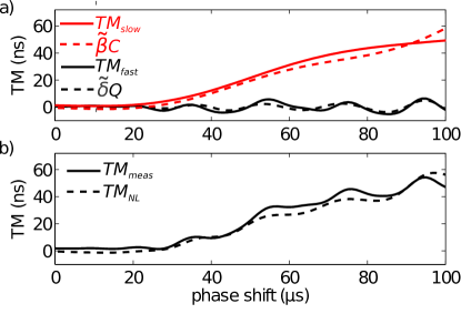
Figure 5: a) The nonlinear parameters $\tilde{\beta}=-872$, $\tilde{\delta}=-1.1\times 10^{10}$ are computed from the fit between $TM_{fast}$ (black line) and $\tilde{\beta}\>Q\left(\phi\right)$ (dashed black) for the fast part, and between $TM_{slow}$ (red line) and $\tilde{\delta}\>C\left(\phi\right)$ (dashed red) for the slow part using Eq. 23 and 22. b) The Time Modulation $TM$ computed from Eq. 18 (dashed line) is in agreement with the measured signal $TM_{meas}$ (solid line).

IV.2 Nonlinear response of a Berea Sandstone

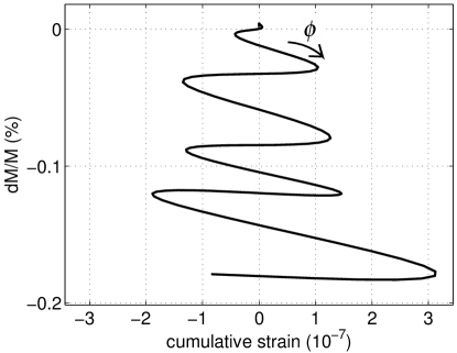
Figure 6: Strain dependency of the elastic modulus : the nonlinear response of a Berea Sandstone is represented as a change in elastic modulus $\nicefrac{{\mathrm{d}M\left(\phi\right)}}{{M}}$ in percent as a function of the cumulative strain $\epsilon\left(\phi\right)=\int_{0}^{L}\epsilon\left(x,\phi+\frac{x}{c_{p}}\right)dx$ for each phase shift $\phi$ value from 0 ($\nicefrac{{\mathrm{d}M\left(\phi\right)}}{{M}}=0$) to 140 ms ($\nicefrac{{\mathrm{d}M\left(\phi\right)}}{{M}}=-0.2\%$). The quadratic non-linearity $\tilde{\beta}$ is responsible for the oscillations and the global trend downward comes from the cubic component $\tilde{\delta}$.

We first explore how the modulus changes with strain. Inverting Eq. 15 shows that the change in elastic modulus is directly related to the relative time modulation as

$$\frac{\mathrm{d}M\left(\phi\right)}{M}\approx-2\frac{TM\left(\phi\right)}{T_{o}}\,.$$ (24)

From this, we compute the change in modulus from the traveltime modulation. To understand the relationship between this change in modulus and the strain, induced by the pump, in the sample, we plot the left-hand side of Eq. 24 as a function of the cumulative pump strain

$$\epsilon\left(\phi\right)=\int_{0}^{L}\epsilon\left(x,\phi+\frac{x}{c_{p}}\right)dx\,.$$ (25)

It is now possible to represent the change of modulus $M$ as a function of the strain. The maximum change is approximately 0.2% of the elastic modulus (c.f. 1), which is similar to observations at large scale during slow slip events Rivet_2011 , earthquakes Brenguier_2008 or volcanism Brenguier_2008a .

The curve shown in figure 6 shows a decrease in $M$ with time ($\phi=0$ is the top of the plot), as well as an increase in the cumulative pump strain. The quadratic term (Eq. 19) is responsible for the small oscillations of the elastic modulus while the cubic term (Eq. 20) explains this global weakening (decrease of $M$) of the material. This weakening is a result of the accumulation of strain over the time that the pump interacts with the sample, and is not evidence of slow-dynamics. More precisely, in Eq. 20 we see that the cubic nonlinearity is governed by the integration of $\epsilon^{2}$ along the path, over time. What we observe in Figure 6 is the increase of this integral with time, i.e. as the pump continues to oscillate within the sample it causes the integral of the square of the strain (Eq. 25) to increase with time. Thus, we are seeing an accumulation of the nonlinear effect as the pump continues to propagate in the sample. In a perfect steady state regime, each oscillation would describe the same curve. This regime is not reached due to the finite size of the sample and the short recording time.

IV.3 Absence of slow-dynamics

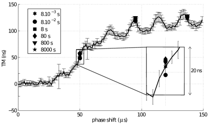
Figure 7: The solid curve shows the time modulation $TM_{meas}$ measured with a delay $8\>\textrm{ms}$ between two pump activations (i.e. the repetition frequency). This is the same curve as 5 b) with a different pump amplitude. An average over 10 acquisitions was performed and the error bars reflect the variation between those acquisitions. The time modulation is shown at 3 phase shift values using delays of activation ranging from $8\>\textrm{ms}$ to 8000 s. The inset gives a closer look at the different delays of acquisition at one phase and shows that the variations for different delays is within the noise of the experiment: there is no slow-dynamic effect in the measurements.

As explained above, the change of elasticity shown in Figure 5 is instantaneous. Nevertheless, as mentioned in the introduction, it is known that the nonlinear response of rocks includes a memory effect as reported by Holcomb for quasi-static measurement Holcomb_1981 , and by TenCate and others TenCate_1996 ; Johnson_2005 for dynamic measurements. After a strong excitation they observed a weakening that decreases with a very slow dynamic process, possibly lasting up to several hours. This time scale can be explored in the present experiment by changing the delay $d_{p}$ between two pump activations. This means that we repeat the experiment at the same $\phi$ and vary the wait time, $d_{p}$ between two experiments. We vary $d_{p}$ from 8 ms to 8000 s. The main curve of Fgure 7 is another acquisition of the time modulation already shown in Figure 5 c), but with a higher pump amplitude. In order to limit the acquisition time, the time modulation is measured at each $d_{p}$ for only 3 phase shifts values. Because of this limited measurement we cannot estimate the nonlinear parameters. Nevertheless, it is clear in Figure 7 that measurements made with different values of the delay $d_{p}$, all fall on the same curve, indicating that the delay does not affect the time modulation $TM_{meas}$, and thus the nonlinear response. It is possible that the maximum strain, on the order of a microstrain, is too small to observe a slow dynamic process; this is of a similar order-of-magnitude to that found in previous studies to cause slow dynamics. For example, Pasqualini et al Pasqualini_2007 report a threshold of around $5\times 10^{-7}$ strain in sandstones to produce a slow-dynamic effect. The main effect of the slow dynamic process is a global weakening described by including a constant in the elastic modulus to strain relationship given in equation 12. Any measurement of $TM_{meas}$ is based on the acquisition of an original probe and a perturbed probe when the pump is turned on (Eq. 1), which picks up a difference between two states and not the absolute magnitude of the perturbation. As a consequence, if there is any slow global weakening it is not measured here. Nevertheless, this observation ensures that the measured parameters $\tilde{\beta}$ and $\tilde{\delta}$ are independent of the time properties of the acquisition sequence.

IV.4 Temperature effects

The nonlinear response of materials are known to be sensitive to environmental parameters. We measured $\tilde{\beta}$ and $\tilde{\delta}$ 300 times with a maximal strain of $2.5\times 10^{-6}$ over a long period of time (14 days) during which the room temperature switched two times from the maximum to the minimum (from $22\,^{\circ}\mathrm{C}$ to $15\,^{\circ}\mathrm{C}$) allowed by the room thermostat. The sample was placed in a isothermal box in order to slow down the change in temperature and damp the fluctuations; a thermometer was also placed in the box to monitor the temperature. Figure 8 shows the evolution of $\tilde{\beta}$ and $\tilde{\delta}$ as a function of the time and thus temperature. The maximum of the cross-correlation between the cubic non-linearity $\tilde{\delta}$ and the temperature is remarkable (0.91), and still important for $\tilde{\beta}$ (0.78). The curious decorrelation in $\tilde{\beta}$ between day 2 and 6 probably involves other experimental parameters such as the humidity and pressure that are also known to perturb the nonlinear response Carpenter_2006 ; Ulrich_2001 .

Another unexplained feature of this experiment is the first measurement of $\tilde{\beta}$ after half a day with no pump on day 7 which is 50% smaller than subsequent points. This bias was noted for all the experiments and for this reason, the first measurement is excluded when an average is performed. This phenomenon is probably related to a slow-dynamic effect with a very long recovery time as it is not observed after 2.2 hours (8000 s) in the previous experiment (Figure 7). Both the effects of temperature decorrelation and first acquisition bias are only present on $\tilde{\beta}$ demonstrating that $\tilde{\beta}$ and $\tilde{\delta}$ are independent and likely have different physical origins. The following section discusses the physical meaning of these nonlinear parameters.

In making these measurements, we were not able to directly monitor the strain amplitude as the laser vibrometer was not available. Estimates of strain are based on the application of the same voltage to the pump transducer as used in previous experiments. Our goal here, is to characterize the effect that varying temperature has on our results. It remains possible that the origin of this effect is not a change in the nonlinearity of the rock itself, but instead a change in the apparatus resulting in a change in the induced pump strain. It is clear, however, that the effect of temperature cannot be ignored; to mitigate this effect in other experiments, we use a combination of shielding to reduce temperature fluctuations and speed to make the measurements as quickly as possible to avoid the effects of such fluctuations on the result. Note also that the large fluctuations shown in Figure 8 are a result of a $\sim 10\,^{\circ}\mathrm{C}$ fluctuation which is significantly more than is usually observed in our laboratory.

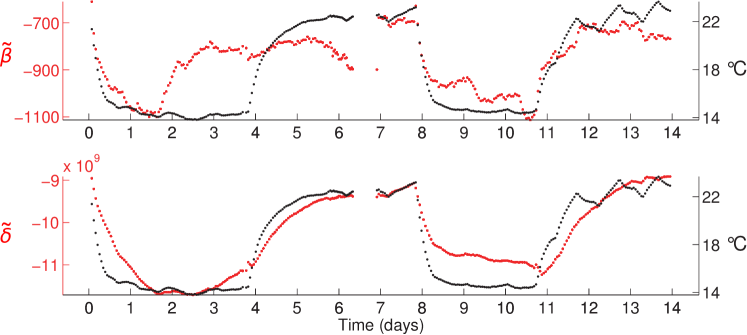
Figure 8: The 14-day evolution of $\tilde{\beta}$, $\tilde{\delta}$ (red dots) and the room temperature (in Celsius, black dots) demonstrates the strong correlation between $\tilde{\delta}$ and the temperature, and a fair correlation between $\tilde{\beta}$ and the temperature.

IV.5 Strain amplitude dependency

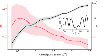
Figure 9: $\tilde{\beta}$ and $\tilde{\delta}$ (respectively red and black) as a function of the maximum induced strain in the sample by different amplitudes of the shear wave pump. Above 0.6 microstrain, $\tilde{\beta}$ decreases with strain whereas $\tilde{\delta}$ increases implying different mechanisms. The abscissa is the maximum of the strain over the whole propagation time of the pump measured along the probe path ($0<x<15$ cm, $0<y<3$ cm, $1.5<z<4.5$ cm). The variation of this maximal strain along the $x$-axis shown in the inset illustrates the inhomogeneous spatial distribution of strain in the sample, obtained from the finite difference simulation.

In the description of the nonlinear parameters given in section III.3, we discuss a nonlinear Hooke’s law. This can, of course, be translated to a wave equation in which the wave speed becomes strain dependent (cf Eq. 9). As a result, the wave propagation becomes strain (or equivalently source amplitude) dependent. For rocks it is reported that the strain wave-speed relationship is itself amplitude dependent meaning that the nonlinear parameters depend on the strain Renaud_2013 . In other words, the nonlinear response of rocks depends on the maximum strain. The nonlinear elastic model is thua valid only at a fixed maximum strain of the pump, and the nonlinear coefficients $\tilde{\beta}$ and $\tilde{\delta}$ are functions of this amplitude.

Our experimental set-up enables the characterization of this feature of the nonlinearities. Estimates of the nonlinear parameters were repeated for 18 pump shear wave amplitudes. The induced strain along the probe path, estimated by the method described in section II.3, attains a maximum ranging from 0.3 to 2.2 microstrain. Figure 9 shows $\tilde{\beta}$ and $\tilde{\delta}$ as a function of the strain and their standard deviation among 300 sets of 18 pump amplitudes. Each set represents one hour of acquisition. The averaging over 300 acquisitions is performed after an adjustment of the median value of each acquisition set in order to remove the environmental effects such as the temperature effects discussed above. The standard deviation is clearly related to the signal to noise ratio as it decreases with increasing pump strain and is much bigger for $\tilde{\beta}$, whose estimation is based on a signal approximately 7 times smaller than that of $\tilde{\delta}$. Figure 9 demonstrates that above a microstrain $\tilde{\delta}$ increases linearly with the strain and $\tilde{\beta}$ decreases linearly with it. The changes are noticeable but remain small for nonlinearities (less than 20%). The quadratic nonlinearity decreases with the absolute strain while the cubic nonlinearity, which is primarily responsible for the rock softening, increases. This is in agreement with the observations of Renaud et al. Renaud_2013 ; Renaud_2013a . The different strain dependencies for the 2 nonlinear parameters suggests that the underlying mechanisms from which the quadratic and cubic nonlinearity originate are different.

The inset in figure 9 shows the spatial distribution of the strain along the probe wave path, modeled with finite difference and scaled to the experiment as described above, and clearly shows that the strain in the medium is not homogeneous. The antisymmetry axis at $x=7.5$ cm is in agreement with the wave response (in strain) to a point force: compression in one half space and tension in the other one. The free boundaries conditions at $x=0$ and $x=15$ cm also have a clear effect on the spatial distribution of strain.

Because of this antisymmetry the maximal strain is only an indicator of the strain amplitude it has to be interpreted carefully when comparing to methods where the strain is nearly uniform. Furthermore, since the nonlinear parameters are amplitude dependent, the spatial distribution of the strain may also affect the measurement, even with the spatio-temporal integration described in Eq. 17.

IV.6 Pump orientation

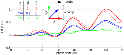
Figure 10: The measured (solid lines) and modeled (dashed lines) time modulations are shown for different values of the angle $\theta$ between the $x$-axis and the orientation of the S-wave transducer $\overrightarrow{p}$. The main pump direction of the strain is indicated by the colored arrows and the probe direction is in black. The red line correspond to the standard case where probe and pump are along the $x$-axis in red (particle motions are aligned). The normalized nonlinear parameters $\tilde{\beta}$ and $\tilde{\delta}$ in the inset show the anisotropy of the nonlinear response.

The shear wave pump creates an anisotropy in the medium, as any uni-axial static load would do (Murnaghan_1951, , p. 64). In other words, the mechanical response of an isotropic medium becomes dependent on the direction of the pump; this effect vanishes when the pump is turned off. In this section we study this effect by changing the direction of the strain pump shear wave particle motion relative to the probe direction. Previously, the propagation of the probe wave and the pump strain occurred in the $x-$direction in the $xz$-plane (Figure 1), i.e. the particle motions of the pump and probe are aligned. It is convenient to change the pump strain direction with a rotation of the pump transducer about the $z-$axis (directed downward in Figure 1). This rotation is a technical challenge of maintaining constant coupling between the S-wave transducer and the sample. We solve this by applying a homogeneous and perfectly oriented force (along the $z-$axis) to the transducer. This force should create a constant coupling, insensitive to a rotation around the $z-$axis. We find the best solution to be a cylindrical load above the transducer with a significant layer of S-wave couplant to provide adequate lubrication during rotation and to minimize the variation in coupling due to drying of the couplant. The rotation of the transducer was carefully performed by small steps in angle to minimize any other perturbation from the change in weight distribution. The stability of the method was checked visually with a transparent sample and quantitatively as described below.

The $x-$component of the displacement was measured with another shear wave transducer placed at the position of the laser beam in Fig. 1: 3 cm under the pump transducer on the $\left(\overrightarrow{z},\overrightarrow{y}\right)$ surface. The measurements of the $x-$component of the displacement for the pump transducer oriented along $\overrightarrow{p}=\mathrm{cos}\theta\>\overrightarrow{x}+\mathrm{sin}\theta\>\overrightarrow{y}$ were found to be close to the projection of $\overrightarrow{p}$ along $\overrightarrow{x}$, within a 10% error. This indicates that the coupling remains relatively constant during the rotation of the pump transducer.

The nonlinear elastic model in Eq. 12 do not includes the $\epsilon_{yz}$ because we noted that this term was negligible (see Eq. 2). When $\theta=\frac{\pi}{2}$, the main component of the displacement is along $y-$axis and $\epsilon_{yz}$ becomes the main strain component. Including this term in the elastic model modifies equation 12 as follows:

$$\frac{\mathrm{d}M}{M} \approx\tilde{\beta}\left(\epsilon_{xx}+\frac{2}{5}\epsilon_{yy}+\frac{2}{5}\epsilon_{zz}\right)$$

$$+ \tilde{\delta}\left(\epsilon_{xx}^{2}+\frac{5}{12}\epsilon_{yy}^{2}+\frac{5}{12}\epsilon_{zz}^{2}+\frac{3}{32}\epsilon_{xz}^{2}+\frac{1}{16}\epsilon_{yz}^{2}\right)\,.$$ (26)

Then, the same procedure described in section II.3 is performed to estimate $\tilde{\beta}$ and $\tilde{\delta}$ as a function of the angle $\theta$. The finite difference simulation was performed for $\theta=[0,\frac{\pi}{4},\frac{\pi}{2}]$ in order to estimate the strain components within the sample and compute the quantities defined in Eq. 19 and 20, with the only change of $\epsilon^{2}=\epsilon_{xx}^{2}+\frac{5}{12}\epsilon_{yy}^{2}+\frac{5}{12}\epsilon_{zz}^{2}+\frac{3}{32}\epsilon_{xz}^{2}+\frac{1}{16}\epsilon_{yz}^{2}$. The nonlinear parameters $\tilde{\beta}$ and $\tilde{\delta}$ are estimated from the measured time modulation using Eq. 22 and 23. Because no laser measurements were available in this experiment, only the relative value of strain is estimated and the nonlinear parameters are normalized by their value at $\theta=0$.

The measured and simulated time modulations are shown in figure 10 and establish the dependency of the nonlinear parameters on the angle $\theta$. No value of $\tilde{\beta}$ is at $\theta=\frac{\pi}{2}$ because the measured fast component of $TM_{meas}$ is very close to the noise level and does not have any phase correlation with the modeled signal. Nevertheless, the value of $\tilde{\beta}(\frac{\pi}{4})=0.7$ indicates that the quadratic nonlinearity decreases when the direction of the particle motion of the pump is orthogonal to that of the probe. On the contrary $\tilde{\delta}(\frac{\pi}{2})=4$ shows an increase of the cubic nonlinearity in this case. This apparent anisotropy has to be considered carefully because, $\tilde{\beta}$ and $\tilde{\delta}$ may vary with the strain distribution (see section III.1). This distribution clearly changes when the pump transducer is rotated and this may bias the anisotropy measurement.

V Conclusion

Previous experiments of nonlinear elastic effects depended on standing waves and finite-sized samples under compressionnal stress. In this work, we demonstrate the feasibility of using two propagating waves for estimating nonlinear properties of a rock. In our experiments, a microstrain pump wave modulates a probe wave; the resulting arrival time modulation was determined to be a cubic function of the complex strain field. The measured time modulation is on the order of tens of nanoseconds, measured in a Berea Sandstone sample with a 50 kHz S-wave pump and a 0.5 MHz P-wave probe. We fit the time modulation data with a two-parameter model: a quadratic and a cubic nonlinearity term related theoretically to averaged elastic moduli of third and fourth order respectively. Temperature, strain amplitude, and the polarization of the pump wave relative to the probe wave direction can affect the measured time delays; longer term slow-dynamic effects do not appear to be significant. Future work will be directed towards investigating larger samples and different types of rocks.

VI Acknowledgments

The authors would like to thank Weatherford, as well as the Earth Resources Laboratory, for funding this research. We are also grateful to Xinding Fang for helping us to setup the modeling code. We thank Jim TenCate and an anonymous reviewer for helpful comments that greatly improved the clarity of the paper.

References

- [1] IY Belyayeva, VY Zaitsev, and AM Sutin. Tomography of nonlinear rock parameters of seismology and seismic prospecting. Fizika Zemli, (12):44–51, DEC 1995.
- [2] RA Guyer and PA Johnson. Nonlinear mesoscopic elasticity: Evidence for a new class of materials. Physics Today, 52(4):30–36, APR 1999.
- [3] Robert A Guyer and Paul A Johnson. Nonlinear mesoscopic elasticity. 2009.
- [4] J. Regnier, L.F. Cadet, H.and Bonilla, E. Bertrand, and J.F. Semblat. Assessing Nonlinear Behavior of Soils in Seismic Site Response: Statistical Analysis on KiK-net Strong-Motion Data. Bulletin of the Seismological Society of America, 103(3):1750–1770, JUN 2013.
- [5] F. Brenguier, M. Campillo, C. Hadziioannou, N. M. Shapiro, R. M. Nadeau, and E. Larose. Postseismic relaxation along the San Andreas fault at Parkfield from continuous seismological observations. Science, 321(5895):1478–1481, SEP 12 2008.
- [6] A Kurtulus and KH Stokoe. In situ measurement of nonlinear shear modulus of silty soil. Journal of geotechnical and geoenvironmental engineering, 134(10):1531–1540, 2008.
- [7] P.A. Johnson, P. Bodin, J. Gomberg, F. Pearce, Z. Lawrence, and F.Y. Menq. Inducing in situ, nonlinear soil response applying an active source. Journal of Geophysical Research: Solid Earth, 114, MAY 21 2009.
- [8] Z. Lawrence, P. Bodin, and Ch.A. Langston. In Situ Measurements of Nonlinear and Nonequilibrium Dynamics in Shallow, Unconsolidated Sediments. Bulletin of the Seismological Society of America, 99(3):1650–1670, JUN 1 2009.
- [9] B.R. Cox, K.H. Stokoe, II, and E.M. Rathje. An In Situ Test Method for Evaluating the Coupled Pore Pressure Generation and Nonlinear Shear Modulus Behavior of Liquefiable Soils. Geotechnical Testing Journal, 32(1):11–21, JAN 2009.
- [10] David J Holcomb. Memory, relaxation, and microfracturing in dilatant rock. Journal of Geophysical Research: Solid Earth, 86(B7):6235–6248, 1981.
- [11] L. Thomsen. Elastic anisotropy due to aligned cracks in porous rock. Geophysical Prospecting, 43(6):805–829, AUG 1995.
- [12] CM SAYERS and M KACHANOV. Microcrack-induced elastic wave anisotropy of brittle rocks. Journal of Geophysical Research: Solid Earth, 100(B3):4149–4156, MAR 10 1995.
- [13] Y Gueguen and A Schubnel. Elastic wave velocities and permeability of cracked rocks. Tectonophysics, 370(1-4):163–176, JUL 31 2003.
- [14] J. Fortin, Y. Gueguen, and A. Schubnel. Effects of pore collapse and grain crushing on ultrasonic velocities and V-p/V-s. Journal of Geophysical Research: Solid Earth, 112(B8), AUG 21 2007.
- [15] P. A Johnson, A. Migliori, and T.J. Shankland. Continuous wave phase detection for probing nonlinear elastic wave interactions in rocks. Journal of the Acoustical Society of America, 89(2):598–603, 1991.
- [16] JA TenCate and TJ Shankland. Slow dynamics in the nonlinear elastic response of Berea sandstone. Geophysical Research Letters, 23(21):3019–3022, OCT 15 1996.
- [17] VE Gusev, W Lauriks, and J Thoen. Dispersion of nonlinearity, nonlinear dispersion, and absorption of sound in micro-inhomogeneous materials. Journal of the Acoustical Society of America, 103(6):3216–3226, JUN 1998.
- [18] RM. D’Angelo, KW. Winkler, TJ. Plona, BJ. Landsberger, and DL. Johnson. Test of hyperelasticity in highly nonlinear solids: Sedimentary rocks. Physical Review Letters, 93(21), 2004.
- [19] T.W. Darling, J.A. TenCate, D.W. Brown, B. Clausen, and S.C. Vogel. Neutron diffraction study of the contribution of grain contacts to nonlinear stress-strain behavior. Geophysical Research Letters, 31(16), AUG 26 2004.
- [20] G. Renaud, S. Calle, J.P. Remenieras, and M. Defontaine. Exploration of trabecular bone nonlinear elasticity using time-of-flight modulation. IEEE Transactions on Ultrasonics Ferroelectrics and Frequency Control, 55(7):1497–1507, 2008. IEEE Ultrasonics Symposium, New York, NY, OCT 28-31, 2007.
- [21] G. Renaud, S. Calle, and M. Defontaine. Remote dynamic acoustoelastic testing: Elastic and dissipative acoustic nonlinearities measured under hydrostatic tension and compression. Applied Physics Letters, 94(1), JAN 5 2009.
- [22] M. Muller, A. Sutin, R. Guyer, M. Talmant, P. Laugier, and P.A. Johnson. Nonlinear resonant ultrasound spectroscopy (nrus) applied to damage assessment in bone. Journal of the Acoustical Society of America, 118:3946, 2005.
- [23] G. Renaud, P. Y. Le Bas, and P. A. Johnson. Revealing highly complex elastic nonlinear (anelastic) behavior of Earth materials applying a new probe: Dynamic acoustoelastic testing. Journal of Geophysical Research: Solid Earth, 117, JUN 6 2012.
- [24] G. Renaud, J. Riviere, S. Haupert, and P. Laugier. Anisotropy of dynamic acoustoelasticity in limestone, influence of conditioning, and comparison with nonlinear resonance spectroscopy. Journal of the Acoustical Society of America, 133(6):3706–3718, JUN 2013.
- [25] G. Renaud, J. Riviere, P. Y. Le Bas, and P. A. Johnson. Hysteretic nonlinear elasticity of Berea sandstone at low-vibrational strain revealed by dynamic acousto-elastic testing. Geophysical Research Letters, 40(4):715–719, FEB 28 2013.
- [26] J Riviere, G Renaud, RA Guyer, and PA Johnson. Pump and probe waves in dynamic acousto-elasticity: Comprehensive description and comparison with nonlinear elastic theories. Journal of Applied Physics, 114(5):054905–054905, 2013.
- [27] G Renaud, J Rivière, C Larmat, JT Rutledge, RC Lee, RA Guyer, K Stokoe, and PA Johnson. In situ characterization of shallow elastic nonlinear parameters with dynamic acoustoelastic testing. Journal of Geophysical Research: Solid Earth, 2014.
- [28] N. Geza, G. Egorov, Y. Mkrtumyan, and V. Yushin. Instantaneous variations in velocity and attenuation of seismic waves in a friable medium in situ under pulsatory dynamic loading: An experimental study,. Russ. Geol. Geophys., 42(7):1079–1087, 2001.
- [29] R. A. Toupin and B. Bernstein. Sound waves in deformed perfectly elastic materials. acoustoelastic effect. The Journal of the Acoustical Society of America, 33(2):216–225, 1961.
- [30] Paul A Johnson and Thomas J Shankland. Nonlinear generation of elastic waves in granite and sandstone: continuous wave and travel time observations. Journal of Geophysical Research: Solid Earth (1978–2012), 94(B12):17729–17733, 1989.
- [31] Michel Destrade, Michael D. Gilchrist, and Raymond W. Ogden. Third- and fourth-order elasticities of biological soft tissues. The Journal of the Acoustical Society of America, 127(4):2103–2106, 2010.
- [32] Michel Destrade, Michael D. Gilchrist, and Giuseppe Saccomandi. Third- and fourth-order constants of incompressible soft solids and the acousto-elastic effect. The Journal of the Acoustical Society of America, 127(5):2759–2763, 2010.
- [33] Michel Destrade and Raymond W. Ogden. On the third- and fourth-order incompressible isotropic elasticity. The Journal of the Acoustical Society of America, 128(6):3334–3343, 2010.
- [34] P Johnson and A Sutin. Slow dynamics and anomalous nonlinear fast dynamics in diverse solids. Journal of the Acoustical Society of America, 117(1):124–130, 2005.
- [35] S. Catheline, F. Wu, and M. Fink. A solution to diffraction biases in sonoelasticity: The acoustic impulse technique. Journal of the Acoustical Society of America, 105 (5):2941–2950, 1999.
- [36] Kenneth W Winkler and Xingzhou Liu. Measurements of third-order elastic constants in rocks. The Journal of the Acoustical Society of America, 100(3):1392–1398, 1996.
- [37] Jean Virieux. P-sv wave propagation in heterogeneous media: Velocity-stress finite-difference method. Geophysics, 51(4):889–901, 1986.
- [38] Robert W Graves. Simulating seismic wave propagation in 3d elastic media using staggered-grid finite differences. Bulletin of the Seismological Society of America, 86(4):1091–1106, 1996.
- [39] LD Landau and EM Lifshitz. Course of Theoretical Physics Vol 7: Theory of Elasticity. Pergamon Press, Oxford, UK, 3rd edition, 1986.
- [40] EA Zabolotskaya. Sound beams in a nonlinear isotropic solid. SOVIET PHYSICS ACOUSTICS-USSR, 32(4):296–299, 1986.
- [41] Xavier Jacob, Stefan Catheline, Jean-Luc Gennisson, Christophe Barriere, Daniel Royer, and Mathias Fink. Nonlinear shear wave interaction in soft solids. Journal of the Acoustical Society of America, 122(4):1917–1926, 2007.
- [42] Zaki Abiza, Michel Destrade, and Ray W Ogden. Large acoustoelastic effect. Wave Motion, 49(2):364–374, 2012.
- [43] M.F. Hamilton, D.T. Blackstock, et al. Nonlinear acoustics. Academic press., 1998.
- [44] G. Renaud, M. Talmant, S. Calle, M. Defontaine, and P. Laugier. Nonlinear elastodynamics in micro-inhomogeneous solids observed by head-wave based dynamic acoustoelastic testing. Journal of the Acoustical Society of America, 130(6):3583–3589, DEC 2011.
- [45] D. Rivet, M. Campillo, N.M. Shapiro, V. Cruz-Atienza, M. Radiguet, N. Cotte, and V. Kostoglodov. Seismic evidence of nonlinear crustal deformation during a large slow slip event in Mexico. Geophysical Research Letters, 38, APR 28 2011.
- [46] F. Brenguier, N.M. Shapiro, M. Campillo, V. Ferrazzini, Z. Duputel, O. Coutant, and A. Nercessian. Towards forecasting volcanic eruptions using seismic noise. Nature Geoscience, 1(2):126–130, 2008.
- [47] D. Pasqualini, K. Heitmann, J.A. TenCate, S. Habib, D.d Higdon, and P.A. Johnson. Nonequilibrium and nonlinear dynamics in Berea and Fontainebleau sandstones: Low-strain regime. Journal of Geophysical Research: Solid Earth, 112(B1), JAN 23 2007.
- [48] M.A. Carpenter, P. Sondergeld, B. Li, R.C. Liebermann, J.W. Walsh, J. Schreuer, and T.W. Darling. Structural evolution, strain and elasticity of perovskites at high pressures and temperatures. Journal of Mineralogical and Petrological Sciences, 101(3):95–109, JUN 2006.
- [49] TJ Ulrich and TW Darling. Observation of anomalous elastic behavior in rock at low temperatures. Geophysical Research Letters, 28(11):2293–2296, JUN 1 2001.
- [50] F.D. Murnaghan. Finite Deformation of an elastic solid. New york John wiley & sons, inc., 1951.