Spectral geometry of the Steklov problem

Abstract.

The Steklov problem is an eigenvalue problem with the spectral parameter in the boundary conditions, which has various applications. Its spectrum coincides with that of the Dirichlet-to-Neumann operator. Over the past years, there has been a growing interest in the Steklov problem from the viewpoint of spectral geometry. While this problem shares some common properties with its more familiar Dirichlet and Neumann cousins, its eigenvalues and eigenfunctions have a number of distinctive geometric features, which makes the subject especially appealing. In this survey we discuss some recent advances and open questions, particularly in the study of spectral asymptotics, spectral invariants, eigenvalue estimates, and nodal geometry.

1. Introduction

1.1. The Steklov problem

Let $\Omega$ be a compact Riemannian manifold of dimension $n\geq 2$ with (possibly non-smooth) boundary $M=\partial\Omega$. The Steklov problem on $\Omega$ is

(1.1.1) $$\begin{cases}\Delta u=0&\mbox{ in }\Omega,\\ \partial_{\nu}u=\sigma\,u&\mbox{ on }M.\end{cases}$$

where $\Delta$ is the Laplace-Beltrami operator acting on functions on $\Omega$, and $\partial_{\nu}$ is the outward normal derivative along the boundary $M$. This problem was introduced by the Russian mathematician V.A. Steklov at the turn of the 20th century (see [69] for a historical discussion). It is well known that the spectrum of the Steklov problem is discrete as long as the trace operator $H^{1}(\Omega)\rightarrow L^{2}(\partial\Omega)$ is compact (see [6]). In this case, the eigenvalues form a sequence $0=\sigma_{0}<\sigma_{1}\leq\sigma_{2}\leq\cdots\nearrow\infty$. This is true under some mild regularity assumptions, for instance if $\Omega$ has Lipschitz boundary (see [77, Theorem 6.2]).

The present paper focuses on the geometric properties of Steklov eigenvalues and eigenfunctions. A lot of progress in this area has been made in the last few years, and some fascinating open problems have emerged. We will start by explaining the motivation to study the Steklov spectrum. In particular, we will emphasize the differences between this eigenvalue problem and its Dirichlet and Neumann counterparts.

1.2. Motivation

The Steklov eigenvalues can be interpreted as the eigenvalues of the Dirichlet-to-Neumann operator ${\mathcal{D}}:H^{1/2}(M)\rightarrow H^{-1/2}(M)$ which maps a function $f\in H^{1/2}(M)$ to ${\mathcal{D}}f=\partial_{\nu}(Hf)$, where $Hf$ is the harmonic extension of $f$ to $\Omega$. The study of the Dirichlet-to-Neumann operator (also known as the voltage-to-current map) is essential for applications to electrical impedance tomography, which is used in medical and geophysical imaging (see [91] for a recent survey).

A rather striking feature of the asymptotic distribution of Steklov eigenvalues is its unusually (compared to the Dirichlet and Neumann cases) high sensitivity to the regularity of the boundary. On one hand, if the boundary of a domain is smooth, the corresponding Dirichlet-to-Neumann operator is pseudodifferential and elliptic of order one (see  [90]). As a result, one can show, for instance, that a surprisingly sharp asymptotic formula for Steklov eigenvalues  (2.1.3) holds for smooth surfaces. However, this estimate already fails for polygons (see section 3). It is in fact likely that for domains which are not $C^{\infty}$-smooth but only of class $C^{k}$ for some $k\geq 1$, the rate of decay of the remainder in eigenvalue asymptotics depends on $k$. To our knowledge, for domains with Lipschitz boundaries, even one-term spectral asymptotics have not yet been proved. A summary of the available results is presented in [2] (see also [3]).

One of the oldest topics in spectral geometry is shape optimization. Here again, the Steklov spectrum holds some surprises. For instance, the classical result of Faber–Krahn for the first Dirichlet eigenvalue $\lambda_{1}(\Omega)$ states that among Euclidean domains with fixed measure, $\lambda_{1}$ is minimized by a ball. Similarly, the Szegő–Weinberger inequality states that the first nonzero Neumann eigenvalue $\mu_{1}(\Omega)$ is maximized by a ball. In both cases, no topological assumptions are made. The analogous result for Steklov eigenvalues is Weinstock’s inequality, which states that among planar domains with fixed perimeter, $\sigma_{1}$ is maximized by a disk provided that $\Omega$ is simply–connected. In contrast with the Dirichlet and Neumann case, this assumption cannot be removed. Indeed the result fails for appropriate annuli (see section 4.2). Moreover, maximization of the first Steklov eigenvalue among all planar domains of given perimeter is an open problem. At the same time, it is known that for simply–connected planar domains, the $k$-th normalized Steklov eigenvalue is maximized in the limit by a disjoint union of $k$ identical disks for any $k\geq 1$ [42]. Once again, for the Dirichlet and Neumann eigenvalues the situation is quite different: the extremal domains for $k\geq 3$ are known only at the level of experimental numerics, and, with a few exceptions, are expected to have rather complicated geometries.

Probably the most well–known question in spectral geometry is “Can one hear the shape of a drum?”, or whether there exist domains or manifolds that are isospectral but not isometric. Apart from some easy examples discussed in section 5, no examples of Steklov isospectral non-isometric manifolds are presently known. Their construction appears to be even trickier than for the Dirichlet or Neumann problems. In particular, it is not known whether there exist Steklov isospectral Euclidean domains which are not isometric. Note that the standard transplantation techniques (see [9, 15, 16]) are not applicable for the Steklov problem, as it is not clear how to “reflect” Steklov eigenfunctions across the boundary.

New challenges also arise in the study of the nodal domains and the nodal sets of Steklov eigenfunctions. One of the problems is to understand whether the nodal lines of Steklov eigenfunctions are dense at the “wave-length scale”, which is a basic property of the zeros of Laplace eigenfunctions. Another interesting question is the nodal count for the Dirichlet-to-Neumann eigenfunctions. We touch upon these topics in section 6.

Let us conclude this discussion by mentioning that the Steklov problem is often considered in the more general form

(1.2.1) $$\partial_{\nu}u=\sigma\rho u,$$

where $\rho\in L^{\infty}(\partial\Omega)$ is a non-negative weight function on the boundary. If $\Omega$ is two-dimensional, the Steklov eigenvalues can be thought of as the squares of the natural frequencies of a vibrating free membrane with its mass concentrated along its boundary with density $\rho$ (see [71]). A special case of the Steklov problem with the boundary condition (1.2.1) is the sloshing problem, which describes the oscillations of fluid in a container. In this case, $\rho\equiv 1$ on the free surface of the fluid and $\rho\equiv 0$ on the walls of the container. There is an extensive literature on the properties of sloshing eigenvalues and eigenfunctions, see [33, 7, 66] and references therein.

Since the present survey is directed towards geometric questions, in order to simplify the analysis and presentation we focus on the pure Steklov problem with $\rho\equiv 1$.

1.3. Computational examples

The Steklov spectrum can be explicitly computed in a few cases. Below we discuss the Steklov eigenvalues and eigenfunctions of cylinders and balls using separation of variables.

Example 1.3.1.

The Steklov eigenvalues of a unit disk are

$$0,1,1,2,2,\dots,k,k,\dots.$$

The corresponding eigenfunctions in polar coordinates $(r,\phi)$ are given by

$$1,r\sin\phi,r\cos\phi,\dots,r\sin k\phi,r\cos k\phi,\dots.$$

Example 1.3.2.

The Steklov eigenspaces on the ball $B(0,R)\subset\mathbb{R}^{n}$ are the restrictions of the spaces $H_{k}^{n}$ of homogeneous harmonic polynomials of degree $l\in\mathbb{N}$ on $\mathbb{R}^{n}$. The corresponding eigenvalue is $\sigma=k/R$ with multiplicity

$$\dim H_{k}^{n}={n+k-1\choose n-1}-{n+k-3\choose n-1}.$$

This is of course a generalization of the previous example.

Example 1.3.3.

This example is taken from [18]. Let $\Sigma$ be a compact Riemannian manifold without boundary. Let

$$0=\lambda_{1}<\lambda_{2}\leq\lambda_{3}\cdots\nearrow\infty$$

be the spectrum of the Laplace-Beltrami operator $\Delta_{\Sigma}$ on $\Sigma$, and let $(u_{k})$ be an orthonormal basis of $L^{2}(\Sigma)$ such that

$$\Delta_{\Sigma}u_{k}=\lambda_{k}u_{k}.$$

Given any $L>0$, consider the cylinder $\Omega=[-L,L]\times\Sigma\subset\mathbb{R}\times\Sigma$. Its Steklov spectrum is given by

$$0,1/L,\ \sqrt{\lambda_{k}}\tanh(\sqrt{\lambda_{k}}L)<\sqrt{\lambda_{k}}\coth(\sqrt{\lambda_{k}}L).$$

and the corresponding eigenfunctions are

$$1,\ t,\ \cosh(\sqrt{\lambda_{k}}t)f_{k}(x),\ \sinh(\sqrt{\lambda_{k}}t)f_{k}(x).$$

In sections 3.1 and 4.2 we will discuss two more computational examples: the Steklov eigenvalues of a square and of annuli.

1.4. Plan of the paper

The paper is organized as follows. In section 2 we survey results on the asymptotics and invariants of the Steklov spectrum on smooth Riemannian manifolds. In section 3 we discuss asymptotics of Steklov eigenvalues on polygons, which turns out to be quite different from the case of smooth planar domains. Section 4 is concerned with geometric inequalities. In section 5 we discuss Steklov isospectrality and spectral rigidity. Finally, section 6 deals with the nodal geometry of Steklov eigenfunctions and the multiplicity bounds for Steklov eigenvalues.

2. Asymptotics and invariants of the Steklov spectrum

2.1. Eigenvalue asymptotics

As above, let $n\geq 2$ be the dimension of the manifold $\Omega$, so that the dimension of the boundary $M=\partial\Omega$ is $n-1$. As was mentioned in the introduction, the Steklov eigenvalues of a compact manifold $\Omega$ with boundary $M=\partial\Omega$ are the eigenvalues of the Dirichlet-to-Neumann map. It is a first order elliptic pseudodifferential operator which has the same principal symbol as the square root of the Laplace-Beltrami operator on $M$. Therefore, applying standard results of Hörmander [56] we obtain the following Weyl’s law for Steklov eigenvalues:

$$\#(\sigma_{j}<\sigma)=\frac{{\rm Vol}(\mathbb{B}^{n-1})\,{\rm Vol}(M)}{(2\pi)^{n-1}}\sigma^{n-1}+{\mathcal{O}}(\sigma^{n-2}),$$

where $\mathbb{B}^{n-1}$ is a unit ball in $\mathbb{R}^{n-1}$. This formula can be rewritten

(2.1.1) $$\sigma_{j}=2\pi\left(\frac{j}{{\rm Vol}(\mathbb{B}^{n-1})\,{\rm Vol}(M)}\right)^{\frac{1}{n-1}}+{\mathcal{O}}(1).$$

In two dimensions, a much more precise asymptotic formula was proved in [41]. Given a finite sequence $C=\{\alpha_{1},\cdots,\alpha_{k}\}$ of positive numbers, consider the following union of multisets (i.e. sets with multiplicities): $\{0,..\dots,0\}\cup\alpha_{1}\mathbb{N}\cup\alpha_{1}\mathbb{N}\cup\alpha_{2}\mathbb{N}\cup\alpha_{2}\mathbb{N}\cup\dots\cup\alpha_{k}\mathbb{N}\cup\alpha_{k}\mathbb{N}$, where the first multiset contains $k$ zeros and $\alpha\mathbb{N}=\{\alpha,2\alpha,3\alpha,\dots,n\alpha,\dots\}$. We rearrange the elements of this multiset into a monotone increasing sequence $S(C)$. For example, $S(\{1\})=\{0,1,1,2,2,3,3,\cdots\}$ and $S(\{1,\pi\})=\{0,0,1,1,2,2,3,3,\pi,\pi,4,4,5,5,6,6,2\pi,2\pi,7,7,\cdots\}$. The following sharp spectral estimate was proved in [41].

Theorem 2.1.2.

Let $\Omega$ be a smooth compact Riemannian surface with boundary $M$. Let $M_{1},\cdots,M_{k}$ be the connected components of the boundary $M=\partial\Omega$, with lengths $\ell(M_{i}),1\leq i\leq k$. Set $R=\left\{\frac{2\pi}{\ell(M_{1})},\cdots,\frac{2\pi}{\ell(M_{k})}\right\}$. Then

(2.1.3) $$\sigma_{j}=S(R)_{j}+{\mathcal{O}}(j^{-\infty}),$$

where $\mathcal{O}(j^{-\infty})$ means that the error term decays faster than any negative power of $j$.

In particular, for simply–connected surfaces we recover the following result proved earlier by Rozenblyum and Guillemin–Melrose (see [83, 25]):

(2.1.4) $$\sigma_{2j}=\sigma_{2j-1}+{\mathcal{O}}(j^{-\infty})=\frac{2\pi}{\ell(M)}j+{\mathcal{O}}(j^{-\infty}).$$

The idea of the proof of Theorem 2.1.2 is as follows. For each boundary component $M_{i}$, $i=1,\dots,k$, we cut off a “collar” neighbourhood of the boundary and smoothly glue a cap onto it. In this way, one obtains $k$ simply–connected surfaces, whose boundaries are precisely $M_{1},\dots,M_{k}$, and the Riemannian metric in the neighbourhood of each $M_{i}$, $i=1,\dots k$, coincides with the metric on $\Omega$. Denote by $\Omega^{*}$ the union of these simply–connected surfaces. Using an explicit formula for the full symbol of the Dirichlet-to-Neumann operator [72] we notice that the Dirichlet-to-Neumann operators associated with $\Omega$ and $\Omega^{*}$ differ by a smoothing operator, that is, by a pseudodifferential operator with a smooth integral kernel; such operators are bounded as maps between any two Sobolev spaces $H^{s}(M)$ and $H^{t}(M)$, $s,t\in\mathbb{R}$. Applying pseudodifferential techniques, we deduce that the corresponding Steklov eigenvalues of $\sigma_{j}(\Omega)$ and $\sigma_{j}(\Omega^{*})$ differ by ${\mathcal{O}}(j^{-\infty})$. Note that a similar idea was used in [55]. Now, in order to study the asymptotics of the Steklov spectrum of $\Omega^{*}$, we map each of its connected components to a disk by a conformal transformation and apply the approach of Rozenblyum-Guillemin-Melrose which is also based on pseudodifferential calculus.

2.2. Spectral invariants

The following result is an immediate corollary of Weyl’s law (2.1.1).

Corollary 2.2.1.

The Steklov spectrum determines the dimension of the manifold and the volume of its boundary.

More refined information can be extracted from the Steklov spectrum of surfaces.

Theorem 2.2.2.

The Steklov spectrum determines the number $k$ and the lengths $\ell_{1}\geq\ell_{2}\geq\cdots\geq\ell_{k}$ of the boundary components of a smooth compact Riemannian surface. Moreover, if $\{\sigma_{j}\}$ is the monotone increasing sequence of Steklov eigenvalues, then:

$$\ell_{1}=\frac{2\pi}{\limsup_{j\rightarrow\infty}(\sigma_{j+1}-\sigma_{j})}.$$

This result is proved in [41] by a combination of Theorem 2.1.2 and certain number-theoretic arguments involving the Dirichlet theorem on simultaneous approximation of irrational numbers.

As was shown in [41], a direct generalization of Theorem 2.2.2 to higher dimensions is false. Indeed, consider four flat rectangular tori: $T_{1,1}=\mathbb{R}^{2}/\mathbb{Z}^{2}$, $T_{2,1}=\mathbb{R}/2\mathbb{Z}\times\mathbb{R}/\mathbb{Z}$, $T_{2,2}~{}=~{}\mathbb{R}^{2}/(2\mathbb{Z})^{2}$ and $T_{\sqrt{2},\sqrt{2}}=\mathbb{R}^{2}/(\sqrt{2}\mathbb{Z})^{2}$. It was shown in [23, 78] that the disjoint union $\mathcal{T}=T_{1,1}\sqcup T_{1,1}\sqcup T_{2,2}$ is Laplace–Beltrami isospectral to the disjoint union $\mathcal{T}^{\prime}=T_{2,1}\sqcup T_{2,1}\sqcup T_{\sqrt{2},\sqrt{2}}$. It follows from Example 1.3.3 that for any $L>0$, the two disjoint unions of cylinders $\Omega_{1}=[0,L]\times\mathcal{T}$ and $\Omega_{2}=[0,L]\times\mathcal{T}^{\prime}$ are Steklov isospectral. At the same time, $\Omega_{1}$ has four boundary components of area $1$ and two boundary components of area $4$, while $\Omega_{2}$ has six boundary components of area $2$. Therefore, the collection of areas of boundary components cannot be determined from the Steklov spectrum. Still, the following question can be asked:

Open Problem 1.

Is the number of boundary components of a manifold of dimension $\geq 3$ a Steklov spectral invariant?

Further spectral invariants can be deduced using the heat trace of the Dirichlet-to-Neumann operator ${\mathcal{D}}$. By the results of [24, 1, 48], the heat trace admits an asymptotic expansion

(2.2.3) $$\sum_{i=0}^{\infty}e^{-t\sigma_{i}}=\operatorname{Tr}e^{-t{\mathcal{D}}}=\int_{M}e^{-t{\mathcal{D}}}(x,x)\ dx\sim\sum_{k=0}^{\infty}a_{k}t^{-n+1+k}+\sum_{l=1}^{\infty}b_{l}t^{l}\log t.$$

The coefficients $a_{k}$ and $b_{l}$ are called the Steklov heat invariants, and it follows from (2.2.3) that they are determined by the Steklov spectrum. The invariants $a_{0},\ldots,a_{n-1}$, as well as $b_{l}$ for all $l$, are local, in the sense that they are integrals over $M$ of corresponding functions $a_{k}(x)$ and $b_{l}(x)$ which may be computed directly from the symbol of the Dirichlet-to-Neumann operator ${\mathcal{D}}$. The coefficients $a_{k}$ are not local for $k\geq n$ [38, 39] and hence are significantly more difficult to study.

In [81], explicit expressions for the Steklov heat invariants $a_{0}$, $a_{1}$ and $a_{2}$ for manifolds of dimensions three or higher were given in terms of the scalar curvatures of $M$ and $\Omega$, as well as the mean curvature and the second order mean curvature of $M$ (for further results in this direction, see [74]). For example, the formula for $a_{1}$ yields the following corollary:

Corollary 2.2.4.

Let $\dim\Omega\geq 3$. Then the integral of the mean curvature over $\partial\Omega=M$ (i.e. the total mean curvature of $M$) is an invariant of the Steklov spectrum.

The Steklov heat invariants will be revisited in section 5.

3. Spectral asymptotics on polygons

The spectral asymptotics given by formula (2.1.1) and Theorem 2.1.2 are obtained using pseudodifferential techniques which are valid only for manifolds with smooth boundaries. In the presence of singularities, the study of the asymptotic distribution of Steklov eigenvalues is more difficult, and the known remainder estimates are significantly weaker (see [2] and references therein). Moreover, Theorem 2.1.2 fails even for planar domains with corners. This can be seen from the explicit computation of the spectrum for the simplest nonsmooth domain: the square.

Eigenspace basis	Conditions on $\alpha$	Eigenvalues	Asymptotic behaviour
$\cos(\alpha x)\cosh(\alpha y)$
$\cos(\alpha y)\cosh(\alpha x)$	$\tan(\alpha)=-\tanh(\alpha)$	$\alpha\tanh(\alpha)$	$\frac{3\pi}{4}+\pi j+{\mathcal{O}}(j^{-\infty})$
$\sin(\alpha x)\cosh(\alpha y)$
$\sin(\alpha y)\cosh(\alpha x)$	$\tan(\alpha)=\coth(\alpha)$	$\alpha\tanh(\alpha)$	$\frac{\pi}{4}+\pi j+{\mathcal{O}}(j^{-\infty})$
$\cos(\alpha x)\sinh(\alpha y)$
$\cos(\alpha y)\sinh(\alpha x)$	$\tan(\alpha)=-\coth(\alpha)$	$\alpha\coth(\alpha)$	$\frac{3\pi}{4}+\pi j+{\mathcal{O}}(j^{-\infty})$
$\sin(\alpha x)\sinh(\alpha y)$
$\sin(\alpha y)\sinh(\alpha x)$	$\tan(\alpha)=\tanh(\alpha)$	$\alpha\coth(\alpha)$	$\frac{\pi}{4}+\pi j+{\mathcal{O}}(j^{-\infty})$
$xy$		1

Table 1. Eigenfunctions obtained by separation of variables on the square $(-1,1)\times(-1,1)$.

3.1. Spectral asymptotics on the square

The Steklov spectrum of the square $\Omega=(-1,1)\times(-1,1)$ is described as follows. For each positive root $\alpha$ of the following equations:

$$\tan(\alpha)+\tanh(\alpha)=0,\quad\tan(\alpha)-\coth(\alpha)=0,$$

$$\tan(\alpha)+\coth(\alpha)=0,\quad\tan(\alpha)-\tanh(\alpha)=0$$

the number $|\alpha\tan(\alpha)|$ is a Steklov eigenvalue of multiplicity two (see Table 1 and Figure 1). The function $f(x,y)=xy$ is also an eigenfunction, with a simple eigenvalue $\sigma_{3}=1$. Starting from $\sigma_{4}$, the normalized eigenvalues are clustered in groups of $4$ around the odd multiples of $2\pi$:

$$\sigma_{4j+l}L=(2j+1)2\pi+{\mathcal{O}}(j^{-\infty}),\qquad\mbox{ for }l=0,1,2,3.$$

This is compatible with Weyl’s law since for $k=4j+l$ it follows that

$$\sigma_{k}L=\left(\frac{k-l}{2}+1\right)2\pi+{\mathcal{O}}(j^{-\infty})=\pi k+{\mathcal{O}}(1).$$

Nevertheless, the refined asymptotics (2.1.4) does not hold.

Let us discuss the spectrum of a square in more detail. Separation of variables quickly leads to the 8 families of Steklov eigenfunctions presented in Table 1 plus an “exceptional” eigenfunction $f(x,y)=xy$.

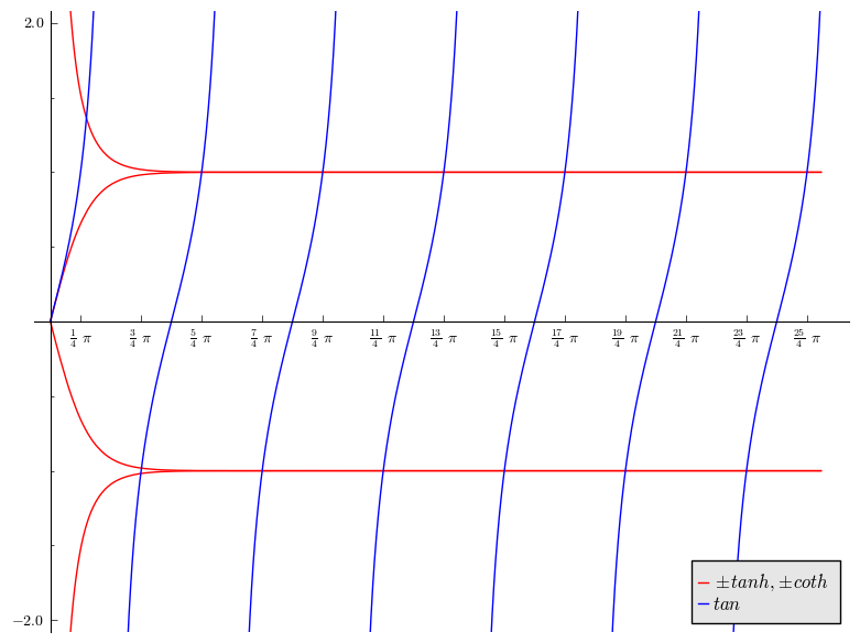
Figure 1. The Steklov eigenvalues of a square. Each intersection corresponds to a double eigenvalue.

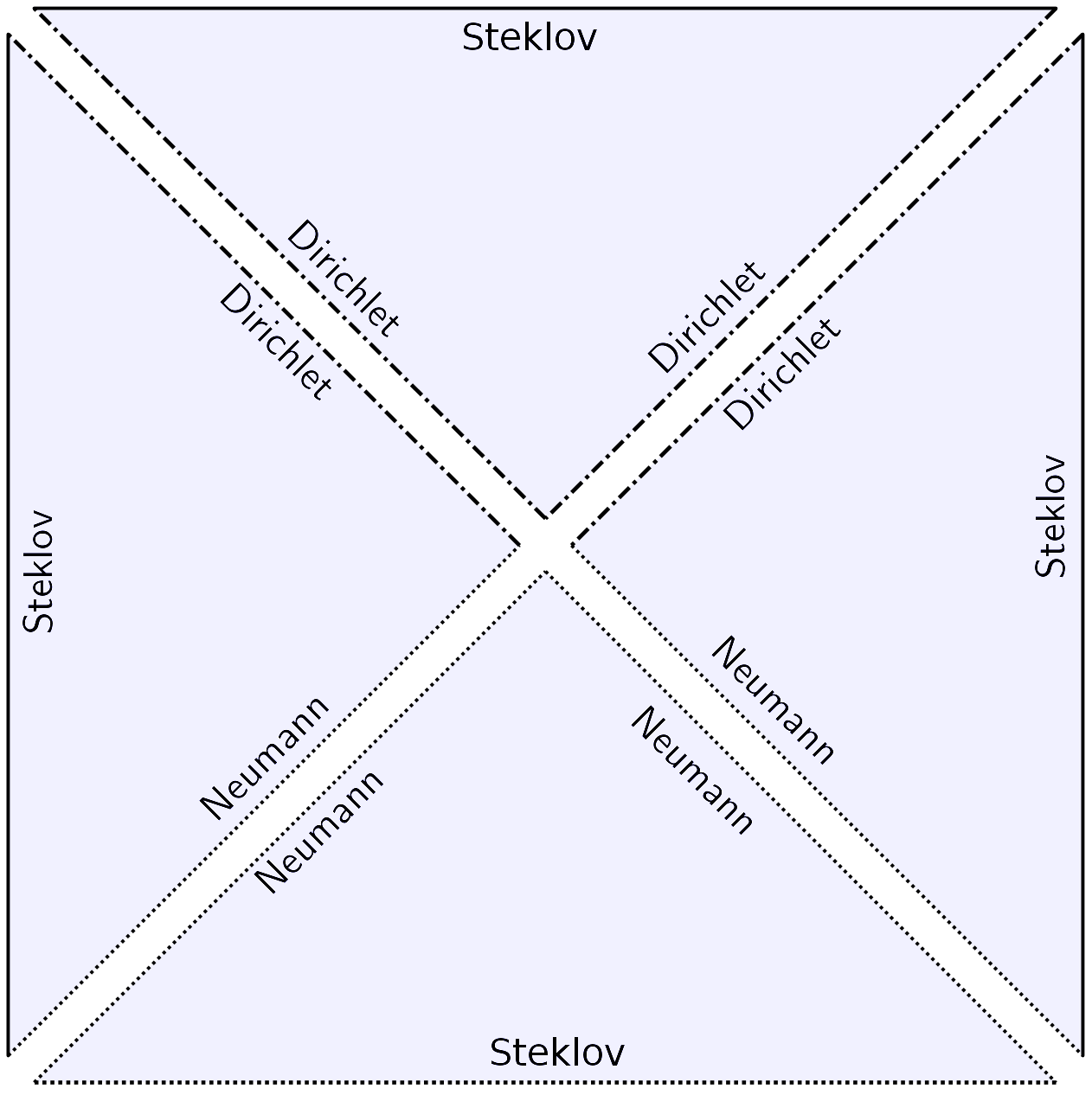
Figure 2. Decomposition of the Steklov problem on a square into four mixed problems on a triangle.

One now needs to prove the completeness of this system of orthogonal functions in $L^{2}(\partial\Omega)$. Using the diagonal symmetries of the square (see Figure 2), we obtain symmetrized functions spanning the same eigenspaces. Splitting the eigenfunctions into odd and even with respect to the diagonal symmetries, we represent the spectrum as the union of the spectra of four mixed Steklov problems on a right isosceles triangle. In each of these problems the Steklov condition is imposed on the hypotenuse, and on each of the sides the condition is either Dirichlet or Neumann, depending on whether the corresponding eigenfunctions are odd or even when reflected across this side. In order to prove the completeness of this system of Steklov eigenfunctions, it is sufficient to show that the corresponding symmetrized eigenfunctions form a complete set of solutions for each of the four mixed problems.

Let us show this property for the problem corresponding to even symmetries across the diagonal. In this way, one gets a sloshing (mixed Steklov–Neumann) problem on a right isosceles triangle. Solutions of this problem were known since 1840s (see [70]). The restrictions of the solutions to the hypotenuse (i.e. to the side of the original square) turn out to be the eigenfunctions of the free beam equation:

$$\frac{d^{4}}{dx^{4}}f=\omega^{4}f\qquad \mbox{ on }(-1,1)$$

$$\frac{d^{3}}{dx^{3}}f=\frac{d^{2}}{dx^{2}}f=0\quad \mbox{ at }x=-1,1.$$

This is a fourth order self-adjoint Sturm-Liouvillle equation. It is known that its solutions form a complete set of functions on the interval $(-1,1)$.

The remaining three mixed problems are dealt with similarly: one reduces the problem to the study of solutions of the vibrating beam equation with either the Dirichlet condition on both ends, or the Dirichlet condition on one end and the Neumann on the other.

3.2. Numerical experiments

Understanding fine spectral asymptotics for the Steklov problem on arbitrary polygonal domains is a difficult question. We have used software from the FEniCS Project (see http://fenicsproject.org/ and [75]) to investigate the behaviour of the Steklov eigenvalues for some specific examples. This was done using an implementation due to B. Siudeja [86] which was already applied in [69]. For the sake of completeness, we discuss two of these experiments here.

Example 3.2.1.

(Equilateral triangle) We have computed the first 60 normalized eigenvalues $\sigma_{j}L$ of an equilateral triangle. The results lead to a conjecture that

$$\sigma_{2j}L=\sigma_{2j+1}L+{\mathcal{O}}(1)=2\pi j+{\mathcal{O}}(1).$$

Example 3.2.2.

(Right isosceles triangle) For the right isosceles triangle with sides of lengths $1,1,\sqrt{2}$, we have also computed the first 60 normalized eigenvalues. The numerics indicate that the spectrum is composed of two sequences of eigenvalues, one of is which behaving as a sequence of double eigenvalues

$$\pi j+{\mathcal{O}}(1)$$

and the other one as a sequence of simple eigenvalues

$$\frac{\pi}{\sqrt{2}}(j+1/2)+{\mathcal{O}}(1).$$

In the context of the sloshing problem, some related conjectures have been proposed in [33].

4. Geometric inequalities for Steklov eigenvalues

4.1. Preliminaries

Let us start with the following simple observation. if a Euclidean domain $\Omega\subset\mathbb{R}^{n}$ is scaled by a factor $c>0$, then

(4.1.1) $$\sigma_{k}(c\,\Omega)=c^{-1}\sigma_{k}(\Omega).$$

Because of this scaling property, maximizing $\sigma_{k}(\Omega)$ among domains with fixed perimeter is equivalent to maximizing the normalized eigenvalues $\sigma_{k}(\Omega)|\partial\Omega|^{1/{(n-1)}}$ on arbitrary domains. Here and further on we use the notation $|\cdot|$ to denote the volume of a manifold.

All the results concerning geometric bounds are proved using a variational characterization of the eigenvalues. Let $\mathcal{E}(k)$ be the set of all $k$ dimensional subspaces of the Sobolev space $H^{1}(\Omega)$ which are orthogonal to constants on the boundary $\partial\Omega$, then

(4.1.2) $$\sigma_{k}(\Omega,g)=\min_{E\in\mathcal{E}(k)}\sup_{0\neq u\in E}R(u),$$

where the Rayleigh quotient is

$$R(u)=\frac{\int_{\Omega}|\nabla u|^{2}\,dA}{\int_{M}u^{2}\,dS}.$$

In particular, the first nonzero eigenvalue is given by

$$\sigma_{1}(\Omega)=\min\Bigl{\{}R(u)\,:\,u\in H^{1}(\Omega),\,\int_{\partial\Omega}u\,dS=0\Bigr{\}}.$$

These variational characterizations are similar to those of Neumann eigenvalues on $\Omega$, where the integral in the denominator of $R(u)$ would be on the domain $\Omega$ rather than on its boundary.

One last observation is in order before we discuss isoperimetric bounds. Let $\Omega_{\epsilon}:=(-1,1)\times(-\epsilon,\epsilon)$ be a thin rectangle ($0<\epsilon<<1$). It is easy to see using using (4.1.2) that

(4.1.3) $$\lim_{\epsilon\rightarrow 0}\sigma_{k}(\Omega_{\epsilon})=0,\qquad\mbox{ for each }k\in\mathbb{N}.$$

In fact, it suffices for a family $\Omega_{\epsilon}$ of domains to have a thin collapsing passage (see Figure 3) to guarantee that $\sigma_{k}(\Omega_{\epsilon})$ becomes arbitrarily small as $\epsilon\searrow 0$ (see [42, section 2.2].)

Figure 3. A domain with a thin passage.

This follows from the variational characterization: the idea is to construct a sequence of $k$ pairwise orthogonal test functions that oscillate inside the thin passage and vanish outside. Then the Dirichlet energy of such functions will be very small, while the denominator in the Rayleigh quotient remains bounded away from zero, due to the integration over the side of the passage. Hence, the Rayleigh quotient will tend to zero, yielding (4.1.3). When considering an isoperimetric constraint, it is therefore more interesting to maximize eigenvalues.

4.2. Isoperimetric upper bounds for Steklov eigenvalues on surfaces

On a compact surface with boundary, the following theorem gives a general upper bound in terms of the genus and the number of boundary components.

Theorem 4.2.1 ([44]).

Let $\Omega$ be a smooth orientable compact surface with boundary $M=\partial\Omega$ of length $L$. Let $\gamma$ be the genus of $\Omega$ and let $l$ be the number of its boundary components. Then the following holds:

(4.2.2) $$\sigma_{p}\sigma_{q}\,L^{2}\leq\begin{cases}\pi^{2}(\gamma+l)^{2}(p+q)^{2}&\mbox{ if }p+q\mbox{ is even},\\ \pi^{2}(\gamma+l)^{2}(p+q-1)^{2}&\mbox{ if }p+q\mbox{ is odd},\end{cases}$$

for any pair of integers $p,q\geq 1$. In particular by setting $p=q=k$ one obtains the following bound:

(4.2.3) $$\sigma_{k}(\Omega)L(M)\leq 2\pi(\gamma+l)k.$$

The proof of Theorem 4.2.1 is based on the existence of a proper holomorphic covering map $\phi:\Omega\rightarrow\mathbb{D}$ of degree $\gamma+l$ (the Ahlfors map), which was proved in [37], and on an ingenious complex analytic argument due to J. Hersch, L. Payne and M. Schiffer [54], who used it to prove inequality (4.2.2) for planar domains. In this particular case, inequality (4.2.3) is known to be sharp. Indeed, it was proved in [42] that equality is attained in the limit by a family $\Omega_{\epsilon}$ of domains degenerating to a disjoint union of $k$ identical disks (see Figure 4).

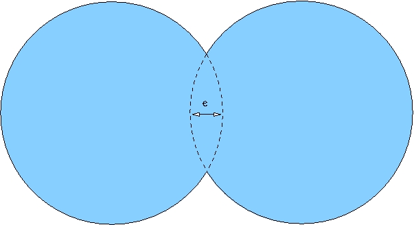
Figure 4. A family of domains $\Omega_{\epsilon}$ maximizing $\sigma_{2}L$ in the limit as $\epsilon\to 0$.

For $k=1$, inequality (4.2.3) was proved in[35].

The earliest isoperimetric inequality for Steklov eigenvalues is that of R. Weinstock [94]. For simply–connected planar domains ($\gamma=0,l=1$), he proved that

(4.2.4) $$\sigma_{1}(\Omega)L(\partial\Omega)\leq 2\pi$$

with equality if and only if $\Omega$ is a disk. Weinstock used an argument similar to that of G. Szegő [89], who obtained an isoperimetric inequality for the first nonzero Neumann eigenvalue of a simply–connected domain $\Omega$ normalized by the measure $|\Omega|$ rather than its perimeter. In fact, Weinstock’s proof is the simplest application of the center of mass renormalization (also known as Hersch’s lemma, see  [53, 84, 40, 43]).

While Szegő’s inequality can be generalized to an arbitrary Euclidean domain (see [93]), this is not true for Weinstock’s inequality. In particular, as follows from the example below, Weinstock’s inequality fails for non-simply–connected planar domains.

Example 4.2.5.

The Steklov eigenvalues and eigenfunctions of an annulus have been computed in [22]. On the annulus $A_{\epsilon}=\mathbb{D}\setminus B(0,\epsilon)$, there is a radially symmetric Steklov eigenfunction

$$f(r)=-\left(\frac{1+\epsilon}{\epsilon\log(\epsilon)}\right)\log(r)+1,$$

with the corresponding eigenvalue $\sigma=\frac{1+\epsilon}{\epsilon\log(1/\epsilon)}$. All other eigenfunctions are of the form

$$f_{k}(r,\theta)=(A_{k}r^{k}+A_{-k}r^{-k})T(k\theta)\qquad(\mbox{with }k\in\mathbb{N})$$

where $T(k\theta)=\cos(k\theta)$ or $T(k\theta)=\sin(k\theta)$. In order for $f_{k}(r,\theta)$ to be a Steklov eigenfunction it is required that

$$\frac{\partial}{\partial_{r}}f_{k}(1,\theta)=\sigma f(1,\theta)\qquad\mbox{ and}\qquad-\frac{\partial}{\partial_{r}}f_{k}(\epsilon,\theta)=\sigma f(\epsilon,\theta),$$

which leads to the following system:

$$\left(\begin{array}[]{cc}\sigma\epsilon^{k}+k\epsilon^{k-1}&\sigma\epsilon^{-k}-k\epsilon^{-k-1}\\ \sigma-k&\sigma+k\end{array}\right)\left(\begin{array}[]{c}A_{k}\\ A_{-k}\end{array}\right)=\left(\begin{array}[]{c}0\\ 0\end{array}\right).$$

This system has a non-zero solution if and only if its determinant vanishes. After some simplifications, the Steklov eigenvalues of the annulus $A_{\epsilon}=\mathbb{D}\setminus B(0,\epsilon)$ are seen to be the roots of the quadratic polynomials

$$p_{k}(\sigma)=\sigma^{2}-\sigma k\left(\frac{\epsilon+1}{\epsilon}\right)\left(\frac{1+\epsilon^{2k}}{1-\epsilon^{2k}}\right)+\frac{1}{\epsilon}k^{2}\qquad(k\in\mathbb{N}).$$

Each of these eigenvalues is double, corresponding to the choice of a $\cos$ or $\sin$ function for the angular part $T(k\theta)$ of the corresponding eigenfunction. For $\epsilon>0$ small enough, this leads in particular to

(4.2.6) $$\sigma_{1}(A_{\epsilon})=\frac{1}{2\epsilon}\frac{1+\epsilon^{2}}{1-\epsilon}\left(1-\sqrt{1-4\epsilon\left(\frac{1-\epsilon}{1+\epsilon^{2}}\right)^{2}}\right).$$

It follows from formula (4.2.6) that for the annulus $A_{\epsilon}=B(0,1)\setminus B(0,\epsilon)$ one has

(4.2.7) $$\sigma_{1}(A_{\epsilon})L(\partial A_{\epsilon})=2\pi\sigma_{1}(\mathbb{D})+2\pi\epsilon+o(\epsilon)\quad\mbox{as }\epsilon\searrow 0.$$

Therefore, $\sigma_{1}(A_{\epsilon})L(\partial A_{\epsilon})>2\pi\sigma_{1}(\mathbb{D})$ for $\epsilon>0$ small enough (see Figure 5), and hence Weinstock’s inequality (4.2.4) fails.

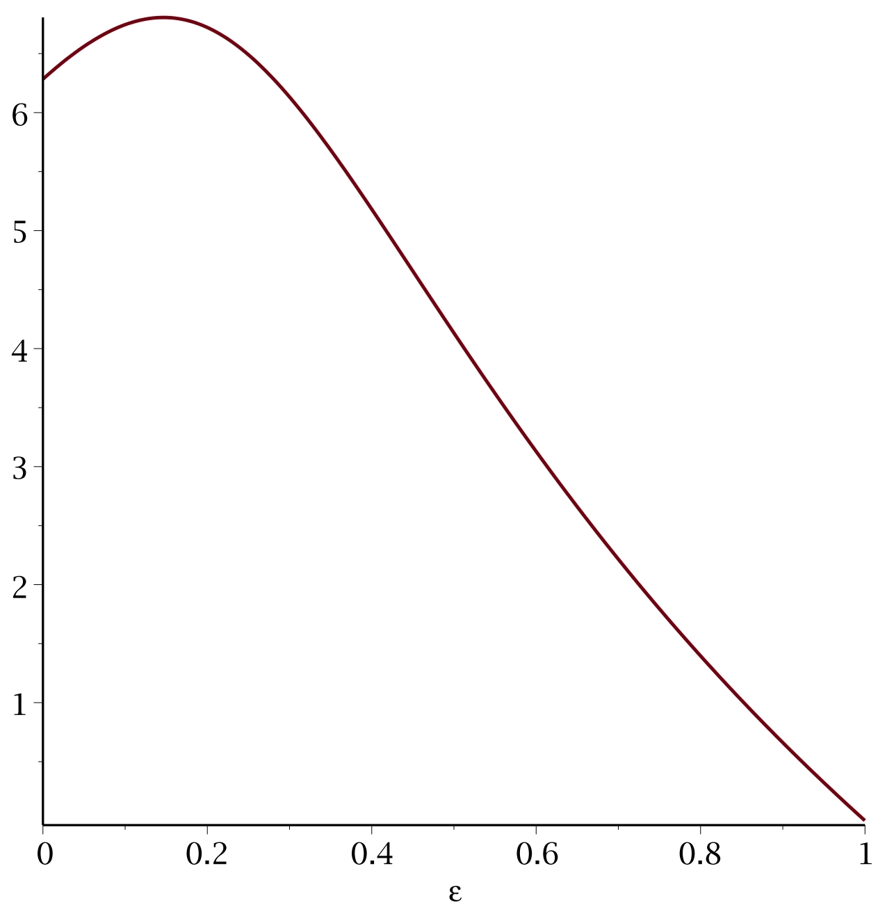
Figure 5. The normalized eigenvalue $\sigma_{1}(A_{\epsilon})L(\partial A_{\epsilon})$

Remark 4.2.8.

One can also compute the Steklov eigenvalues of the spherical shell $\Omega_{\epsilon}:=B(0,1)\setminus B(0,\epsilon)\subset\mathbb{R}^{n}$ for $n\geq 3$. The eigenvalues are the roots of certain quadratic polynomials which can be computed explicitly. Here again, it is true that for $\epsilon>0$ small enough, $\sigma_{1}(\Omega_{\epsilon})|\partial\Omega_{\epsilon}|^{\frac{1}{n-1}}>\sigma_{1}(\mathbb{B})|\partial\mathbb{B}|^{\frac{1}{n-1}}$. This computation was part of an undergraduate research project of E. Martel at Université Laval.

Given that Weinstock’s inequality is no longer true for non-simply–connected planar domains, one may ask whether the supremum of $\sigma_{1}L$ among all planar domains of fixed perimeter is finite. This is indeed the case, as follows from the following theorem for $k=1$ and $\gamma=0$.

Theorem 4.2.9 ([18]).

There exists a universal constant $C>0$ such that

(4.2.10) $$\sigma_{k}(\Omega)L(\partial\Omega)\leq C(\gamma+1)k.$$

Theorem 4.2.9 leads to the the following question:

Open Problem 2.

What is the maximal value of $\sigma_{1}(\Omega)$ among Euclidean domains $\Omega\subset\mathbb{R}^{n}$ of fixed perimeter? On which domain (or in the limit of which sequence of domains) is it realized?

Some related results will be discussed in subsection 4.3. In particular, in view of Theorem 4.3.5 [35], it is tempting to suggest that the maximum is realized in the limit by a sequence of domains with the number of boundary components tending to infinity.

The proof of Theorem 4.2.9 is based on N. Korevaar’s metric geometry approach [65] as described in [47]. For $k=1$, inequality (4.2.10) holds with $C=8\pi$ (see [64]). For $k=1$ and $\gamma=0$, it holds with $C=4\pi$ [35] (see Theorem 4.3.5 below). It is also possible to “decouple” the genus $\gamma$ and the index $k$. The following theorem was proved by A. Hassannezhad [51], using a generalization of the Korevaar method in combination with concentration results from [20].

Theorem 4.2.11.

There exists two constants $A,B>0$ such that

$$\sigma_{k}(\Omega)L(\partial\Omega)\leq A\gamma+Bk.$$

At this point, we have considered maximization of the Steklov eigenvalues under the constraint of fixed perimeter. This is natural, since they are the eigenvalues of to the Dirichlet-to-Neumann operator, which acts on the boundary. Nevertheless, it is also possible to normalize the eigenvalues by fixing the measure of $\Omega$. The following theorem was proved by F. Brock [14].

Theorem 4.2.12.

Let $\Omega\subset\mathbb{R}^{n}$ be a bounded Lipschitz domain. Then

(4.2.13) $$\sigma_{1}(\Omega)|\Omega|^{1/n}\leq\omega_{n}^{1/n},$$

with equality if and only if $\Omega$ is a ball. Here $\omega_{n}$ is the volume of the unit ball $\mathbb{B}^{n}\subset\mathbb{R}^{n}$.

Observe that no connectedness assumption is required this time. The proof of Theorem 4.2.12 is based on a weighted isoperimetric inequality for moments of inertia of the boundary $\partial\Omega$. A quantitative improvement of Brock’s theorem was obtained in [13] in terms of the Fraenkel asymmetry of a bounded domain $\Omega\subset\mathbb{R}^{n}$:

$$\mathcal{A}(\Omega):=\inf\left\{\frac{\|1_{\Omega}-1_{B}\|_{L^{1}}}{|\Omega|}\,:\,B\mbox{ is a ball with }|B|=|\Omega|\right\}.$$

Theorem 4.2.14.

Let $\Omega\subset\mathbb{R}^{n}$ be a bounded Lipschitz domain. Then

(4.2.15) $$\sigma_{1}(\Omega)|\Omega|^{1/n}\leq\omega_{n}^{1/n}(1-\alpha_{n}\mathcal{A}(\Omega)^{2}),$$

where $\alpha_{n}>0$ depends only on the dimension.

The proof of Theorem 4.2.14 is based on a quantitative refinement of the isoperimetric inequality. It would be interesting to prove a similar stability result for Weinstock’s inequality:

Open Problem 3.

Let $\Omega$ be a planar simply–connected domain such that the difference $2\pi-\sigma_{1}(\Omega)L(\partial\Omega)$ is small. Show that $\Omega$ must be close to a disk (in the sense of Fraenkel asymmetry or some other measure of proximity).

4.3. Existence of maximizers and free boundary minimal surfaces

A free boundary submanifold is a proper minimal submanifold of some unit ball $\mathbb{B}^{n}$ with its boundary meeting the sphere $\mathbb{S}^{n-1}$ orthogonally. These are characterized by their Steklov eigenfunctions.

Lemma 4.3.1 ([34]).

A properly immersed submanifold $\Omega$ of the ball $\mathbb{B}^{n}$ is a free boundary submanifold if and only if the restriction to $\Omega$ of the coordinate functions $x_{1},\cdots,x_{n}$ satisfy

$$\begin{cases}\Delta x_{i}=0&\mbox{ in }\Omega,\\ \partial_{\nu}x_{i}=\,x_{i}&\mbox{ on }\partial\Omega.\end{cases}$$

This link was exploited by A. Fraser and R. Schoen who developed the theory of extremal metrics for Steklov eigenvalues. See [34, 35] and especially [36] where an overview is presented.

Let $\sigma^{\star}(\gamma,k)$ be the supremum of $\sigma_{1}L$ taken over all Riemannian metrics on a compact surface of genus $\gamma$ with $l$ boundary components. In [35], a geometric characterization of maximizers was proved.

Proposition 4.3.2.

Let $\Omega$ be a compact surface of genus $\gamma$ with $l$ boundary components and let $g_{0}$ be a smooth metric on $\Omega$ such that

$$\sigma_{1}(\Omega,g_{0})L(\partial\Omega,g_{0})=\sigma^{\star}(\gamma,l).$$

Then there exist eigenfunctions $u_{1},\cdots,u_{n}$ corresponding to $\sigma_{1}(\Omega)$ such that the map

$$u=(u_{1},\cdots,u_{n}):\Omega\rightarrow\mathbb{B}^{n}$$

is a conformal minimal immersion such that $u(\Omega)\subset\mathbb{B}^{n}$ is a free boundary solution, and is an isometry on $\partial\Omega$ up to a rescaling by a constant factor.

This result was extended to higher eigenvalues $\sigma_{k}$ in [36]. This characterization is similar to that of extremizers of the eigenvalues of the Laplace operator on surfaces (see [76, 27, 28]).

For surfaces of genus zero, Fraser and Schoen could also obtain an existence and regularity result for maximizers, which is the main result of their paper [35].

Theorem 4.3.3.

For each $l>0$, there exists a smooth metric $g$ on the surface of genus zero with $l$ boundary components such that

$$\sigma_{1}(\Omega,g)L_{g}(\partial\Omega)=\sigma^{\star}(0,l).$$

Similar existence results have been proved for the first nonzero eigenvalue of the Laplace–Beltrami operator in a fixed conformal class of a closed surface of arbitrary genus, in which case conical singularities have to be allowed (see [58, 80]).

Proposition 4.3.2 and Theorem 4.3.3 can be used to study optimal upper bounds for $\sigma_{1}$ on surfaces of genus zero. Observe that inequality (4.2.3) can be restated as

$$\sigma^{\star}(\gamma,l)\leq 2\pi(\gamma+l).$$

This bound is not sharp in general. For instance, Fraser and Schoen [35] proved that on annuli ($\gamma=0,l=2$), the maximal value of $\sigma_{1}(\Omega)L(\partial\Omega)$ is attained by the critical catenoid ($\sigma_{1}L\sim 4\pi/1.2$), which is the minimal surface $\Omega\subset B^{3}$ parametrized by

$$\phi(t,\theta)=c(\cosh(t)\cos(\theta),\cosh(t)\sin(\theta),t),$$

where the scaling factor $c>0$ is chosen so that the boundary of the surface $\Omega$ meets the sphere $\mathbb{S}^{2}$ orthogonally.

Theorem 4.3.4 ([35]).

The supremum of $\sigma_{1}(\Omega)L(\partial\Omega)$ among surfaces of genus 0 with two boundary components is attained by the critical catenoid. The maximizer is unique up to conformal changes of the metric which are constant on the boundary.

The uniqueness statement is proved using Proposition 4.3.2 by showing that the critical catenoid is the unique free boundary annulus in a Euclidean ball. The maximization of $\sigma_{1}L$ for the Möbius bands has also been considered in [35].

For surfaces of genus zero with arbitrary number of boundary components, the maximizers are not known explicitly, but the asymptotic behaviour for large number of boundary components is understood [35].

Theorem 4.3.5.

The sequence $\sigma^{\star}(0,l)$ is strictly increasing and converges to $4\pi$. For each $l\in\mathbb{N}$ a maximizing metric is achieved by a free boundary minimal surface $\Omega_{l}$ of area less than $2\pi$. The limit of these minimal surfaces as $l\nearrow+\infty$ is a double disk.

The results discussed above lead to the following question:

Open Problem 4.

Let $\Omega$ be a surface of genus $\gamma$ with $l$ boundary components. Does there exist a smooth Riemannian metric $g_{0}$ such that

$$\sigma_{1}(\Omega,g_{0})L(\partial\Omega,g_{0})\geq\sigma_{1}(\Omega,g)L(\partial\Omega,g)$$

for each Riemannian metric $g$?

Free boundary minimal surfaces were used as a tool in the study of maximizers for $\sigma_{1}$, but this interplay can be turned around and used to obtain interesting geometric results.

Corollary 4.3.6.

For each $l\geq 1$, there exists an embedded minimal surface of genus zero in $\mathbb{B}^{3}$ with $l$ boundary components satisfying the free boundary condition.

4.4. Geometric bounds in higher dimensions

In dimensions $n=\mbox{dim}(\Omega)\geq 3$, isoperimetric inequalities for Steklov eigenvalues are more complicated, as they involve other geometric quantities, such as the isoperimetric ratio:

$$I(\Omega)=\frac{|M|}{|\Omega|^{\frac{n-1}{n}}}.$$

For the first nonzero eigenvalue $\sigma_{1}$, it is possible to obtain upper bounds for general compact manifolds with boundary in terms of $I(\Omega)$ and of the relative conformal volume, which is defined below. Let $\Omega$ be a compact manifold of dimension $n$ with smooth boundary $M$. Let $m\in\mathbb{N}$ be a positive integer. The relative $m$-conformal volume of $\Omega$ is

$$V_{rc}(\Omega,m)=\inf_{\phi:\Omega\hookrightarrow B^{m}}\sup_{\gamma\in M(m)}\mbox{Vol}(\gamma\circ\phi(\Omega)),$$

where the infimum is over all conformal immersions $\phi:\Omega\hookrightarrow\mathbb{B}^{m}$ such that $\phi(M)\subset\partial\mathbb{B}^{m}$, and $M(m)$ is the group of conformal diffeomorphisms of the ball. This conformal invariant was introduced in  [34]. It is similar to the celebrated conformal volume of P. Li and S.-T. Yau [73].

Theorem 4.4.1.

[34] Let $\Omega$ be a compact Riemannian manifold of dimension $n$ with smooth boundary $M$. For each positive integer $m$, the following holds:

(4.4.2) $$\sigma_{1}(\Omega)|M|^{\frac{1}{n-1}}\leq\frac{nV_{rc}(\Omega,m)^{2/n}}{I(\Omega)^{\frac{n-2}{n-1}}}.$$

In case of equality, there exists a conformal harmonic map $\phi:\Omega\rightarrow\mathbb{B}^{m}$ which is a homothety on $M=\partial\Omega$ and such that $\phi(\Omega)$ meets $\partial B^{m}$ orthogonally. If $n\geq 3$, then $\phi$ is is an isometric minimal immersion of $\Omega$ and it is given by a subspace of the first eigenspace.

The proof uses coordinate functions as test functions and is based on the Hersch center of mass renormalization procedure. It is similar to the proof of the Li-Yau inequality [73].

For higher eigenvalues, the following upper bound for bounded domains was proved by B. Colbois, A. El Soufi and the first author in [18].

Theorem 4.4.3.

Let $N$ be a Riemannian manifold of dimension $n$. If $N$ is conformally equivalent to a complete Riemannian manifold with non-negative Ricci curvature, then for each domain $\Omega\subset N$, the following holds for each $k\geq 1$,

(4.4.4) $$\sigma_{k}(\Omega)|M|^{\frac{1}{n-1}}\leq\frac{\alpha(n)}{I(\Omega)^{\frac{n-2}{n-1}}}k^{2/n}.$$

where $\alpha(n)$ is a constant depending only $n$.

The proof of Theorem 4.4.3 is based on the methods of metric geometry initiated in [65] and further developed in [47]. In combination with the classical isoperimetric inequality, Theorem 4.4.3 leads to the following corollary.

Corollary 4.4.5.

There exists a constant $C_{n}$ such that for any Euclidean domain $\Omega\subset\mathbb{R}^{n}$

$$\sigma_{k}(\Omega)|\partial\Omega|^{\frac{1}{n-1}}\leq C_{n}k^{2/n}.$$

Similar results also hold for domains in the hyperbolic space $\mathbb{H}^{n}$ and in the hemisphere of $\mathbb{S}^{n}$. An interesting question raised in [18] is whether one can replace the exponent $2/n$ in Corollary 4.4.5 by $1/(n-1)$, which should be optimal in view of Weyl’s law (2.1.1):

Open Problem 5.

Does there exist a constant $C_{n}$ such that any bounded Euclidean domain $\Omega\subset\mathbb{R}^{n}$ satisfies

$$\sigma_{k}(\Omega)|\partial\Omega|^{\frac{1}{n-1}}\leq C_{n}k^{\frac{1}{n-1}}?$$

While it might be tempting to think that inequality (4.4.4) should also hold with the exponent $1/(n-1)$, this is false since it would imply a universal upper bound on the isoperimetric ratio $I(\Omega)$ for Euclidean domains.

4.5. Lower bounds

In [29], J. Escobar proved the following lower bound.

Theorem 4.5.1.

Let $\Omega$ be a smooth compact Riemannian manifold of dimension $\geq 3$ with boundary $M=\partial\Omega$. Suppose that the Ricci curvature of $\Omega$ is non-negative and that the second fundamental form of $M$ is bounded below by $k_{0}>0$, then $\sigma_{1}>k_{0}/2.$

The proof is a simple application of Reilly’s formula. In [30], Escobar conjectured the stronger bound $\sigma_{1}\geq k_{0}$, which he proved for surfaces. For convex planar domains, this had already been proved by Payne [79]. Earlier lower bounds for convex and starshaped planar domains are due to Kuttler and Sigillito [68, 67].

In more general situations (e.g. no convexity assumption), it is still possible to bound the first eigenvalue from below, similarly to the classical Cheeger inequality. The classical Cheeger constant associated to a compact Riemannian manifold $\Omega$ with boundary $M=\partial\Omega$ is defined by

$$h_{c}(\Omega):=\inf_{|A|\leq\frac{|\Omega|}{2}}\frac{|\partial A\cap\mbox{int }\Omega|}{|A|}.$$

where the infimum is over all Borel subsets of $\Omega$ such that $|A|\leq|\Omega|/2$. In [60] P. Jammes introduced the following Cheeger type constant for the Steklov problem:

$$h_{\mbox{j}}(\Omega):=\inf_{|A|\leq\frac{|\Omega|}{2}}\frac{|\partial A\cap\mbox{int }\Omega|}{|A\cap\partial\Omega|}.$$

He proved the following lower bound.

Theorem 4.5.2.

Let $\Omega$ be a smooth compact Riemannian manifold with boundary $M=\partial\Omega$. Then

(4.5.3) $$\sigma_{1}(\Omega)\geq\frac{1}{4}h_{c}(\Omega)h_{j}(\Omega)$$

The proof of this theorem uses the coarea formula and follows the proof of the classical Cheeger inequality quite closely. Previous lower bounds were also obtained in [29] in terms of a related Cheeger type constant and of the first eigenvalue of a Robin problem on $\Omega$.

4.6. Surfaces with large Steklov eigenvalues

The previous discussion immediately raises the question of whether there exist surfaces with an arbitrarily large normalized first Steklov eigenvalue. The question was settled by the first author and B. Colbois in [19].

Theorem 4.6.1.

There exists a sequence $\{\Omega_{N}\}_{N\in\mathbb{N}}$ of compact surfaces with boundary and a constant $C>0$ such that for each $N\in\mathbb{N}$, $\mbox{genus}(\Omega_{N})=1+N,$ and

$$\sigma_{1}(\Omega_{N})L(\partial\Omega_{N})\geq CN.$$

The proof is based on the construction of surfaces which are modelled on a family of expander graphs.

Remark 4.6.2.

The literature on geometric bounds for Steklov eigenvalues is expanding rather fast. There is some interest in considering the maximization of various functions of the Steklov eigenvalues. See [22, 26, 52]. In the framework of comparison geometry, $\sigma_{1}$ was studied is [31] and more recently in [12]. For submanifolds of $\mathbb{R}^{n}$, upper bounds involving the mean curvatures of $M=\partial\Omega$ have been obtained in [57]. Higher eigenvalues on annuli have been studied in [32].

5. Isospectrality and spectral rigidity

5.1. Isospectrality and the Steklov problem

Adapting the celebrated question of M. Kac “Can one hear the shape of a drum?” to the Steklov problem, one may ask:

Open Problem 6.

Do there exist planar domains which are not isometric and have the same Steklov spectrum?

We believe the answer to this question is negative. Moreover, the problem can be viewed as a special case of a conjecture put forward in [62]: two surfaces have the same Steklov spectrum if and only if there exists a conformal mapping between them such that the conformal factor on the boundary is identically equal to one. Note that the “if” part immediately follows from the variational principle (4.1.2). Indeed, the numerator of the Rayleigh quotient for Steklov eigenvalues is the usual Dirichlet energy, which is invariant under conformal transformations in two dimensions. The denominator also stays the same if the conformal factor is equal to one on the boundary. Therefore, the Steklov spectra of such conformally equivalent surfaces coincide.

In higher dimensions, the Dirichlet energy is not conformally invariant, and therefore the approach described above does not work. However, one can construct Steklov isospectral manifolds of dimension $n\geq 3$ with the help of Example 1.3.3. Indeed, given two compact manifolds $M_{1}$ and $M_{2}$ which are Laplace-Beltrami isospectral (there are many known examples of such pairs, see, for instance, [15, 88, 46]), consider two cylinders $\Omega_{1}=M_{1}\times[0,L]$ and $\Omega_{2}=M_{2}\times[0,L]$, $L>0$. It follows from Example 1.3.3 that $\Omega_{1}$ and $\Omega_{2}$ have the same Steklov spectra. Recently, examples of higher-dimesional Steklov isospectral manifolds with connected boundaries were announced in [45].

In all known constructions of Steklov isospectral manifolds, their boundaries are Laplace isospectral. The following question was asked in [41]:

Open Problem 7.

Do there exist Steklov isospectral manifolds such that their boundaries are not Laplace isospectral?

5.2. Rigidity of the Steklov spectrum: the case of a ball

It is an interesting and challenging question to find examples of manifolds with boundary that are uniquely determined by their Steklov spectrum. In this subsection we discuss the seemingly simple example of Euclidean balls.

Proposition 5.2.1.

A disk is uniquely determined by its Steklov spectrum among all smooth Euclidean domains.

Proof.

Let $\Omega$ be an Euclidean domain which has the same Steklov spectrum as the disk of radius $r$. Then, by Corollary 2.2.1 one immediately deduces that $\Omega$ is a planar domain of perimeter $2\pi r$. Moreover, it follows from Theorem 2.2.2 that $\Omega$ is simply–connected. Therefore, since the equality in Weinstock’s inequality (4.2.4) is achieved for $\Omega$, the domain $\Omega$ is a disk of radius $r$. ∎

Remark 5.2.2.

The smoothness hypothesis in the proposition above seems to be purely technical. We have to make this assumption since we make use of Theorem 2.2.2.

The above result motivates

Open Problem 8.

Let $\Omega\subset{\mathbb{R}}^{n}$ be a domain which is isospectral to a ball of radius $r$. Show that it is a ball of radius $r$.

Note that Theorem 4.2.12 does not yield a solution to this problem because the volume $|\Omega|$ is not a Steklov spectrum invariant. Using the heat invariants of the Dirichlet-to-Neumann operator (see subsection 2.2), one can prove the following statement in dimension three.

Proposition 5.2.3.

Let $\Omega\subset\mathbb{R}^{3}$ be a domain with connected and smooth boundary $M$. Suppose its Steklov spectrum is equal to that of a ball of radius $r$. Then $\Omega$ is a ball of radius $r$.

This result was obtained in [81], and we sketch its proof below. First, let us show that $M$ is simply–connected. We use an adaptation of a theorem of Zelditch on multiplicities [96] proved using microlocal analysis. Namely, since $\Omega$ is Steklov isospectral to a ball, the multiplicities of its Steklov eigenvalues grow as $m_{k}=Ck+{\mathcal{O}}(1)$, where $C>0$ is some constant and $m_{k}$ is the multiplicity of the $k$-th distinct eigenvalue (cf. Example 1.3.2). Then one deduces that $M$ is a Zoll surface (that is, all geodesics on $M$ are periodic with a common period), and hence it is simply–connected [10].

Therefore, the following formula holds for the coefficient $a_{2}$ in the Steklov heat trace asymptotics (2.2.3) on $\Omega$:

$$a_{2}=\frac{1}{16\pi}\int_{M}H_{1}^{2}+\frac{1}{12}.$$

Here $H_{1}(x)$ denotes the mean curvature of $M$ at the point $x$, and the term $\frac{1}{12}$ is obtained from the Gauss–Bonnet theorem using the fact that $M$ is simply–connected. We have then: $\int_{M}H_{1}^{2}=\int_{S_{r}}H_{1}^{2}$, where $S_{r}=\partial B_{r}$.

On the other hand, it follows from (2.1.1) and Corollary 2.2.4 that ${\rm Vol}(M)$ and $\int_{M}H_{1}$ are Steklov spectral invariants. Therefore,

$${\rm Area}(M)={\rm Area}(S_{r}),\,\,\,\int_{M}H_{1}=\int_{S_{r}}H_{1}.$$

Hence

$$\sqrt{{\rm Area}(M)}\left(\int_{M}H_{1}^{2}\right)^{1/2}-\left|\int_{M}H_{1}\right|=\sqrt{{\rm Area}(S_{r})}\left(\int_{S_{r}}H_{1}^{2}\right)^{1/2}-\left|\int_{S_{r}}H_{1}\right|=0.$$

Since the Cauchy-Schwarz inequality becomes an equality only for constant functions, one gets that $H_{1}$ must be constant on $M$. By a theorem of Alexandrov [5], the only compact surfaces of constant mean curvature embedded in $\mathbb{R}^{3}$ are round spheres. We conclude that $M$ is itself a sphere of radius $r$ and therefore $\Omega$ is isometric to $B_{r}$. This completes the proof of the proposition.

6. Nodal geometry and multiplicity bounds

6.1. Nodal domain count

The study of nodal domains and nodal sets of eigenfunctions is probably the oldest topic in geometric spectral theory, going back to the experiments of E. Chladni with vibrating plates. The fundamental result in the subject is Courant’s nodal domain theorem which states that the $n$-th eigenfunction of the Dirichlet boundary value problem has at most $n$ nodal domains. The proof of this statement uses essentially two ingredients: the variational principle and the unique continuation for solutions of second order elliptic equations. It can therefore be extended essentially verbatim to Steklov eigenfunctions (see [68, 63]).

Theorem 6.1.1.

Let $\Omega$ be a compact Riemannian manifold with boundary and $\phi_{n}$ be an eigenfunction corresponding to the $n$-th nonzero Steklov eigenvalue $\sigma_{n}$. Then $\phi_{n}$ has at most $n+1$ nodal domains.

Note that the Steklov spectrum starts with $\sigma_{0}=0$, and therefore the $n$-th nonzero eigenvalue is actually the $n+1$-st Steklov eigenvalue.

Apart of the “interior” nodal domains and nodal sets of Steklov eigenfunctions, a natural problem is to study the boundary nodal domains and nodal sets, that is, the nodal domains and nodal sets of the eigenfunctions of the Dirichlet-to-Neumann operator.

The proof of Courant’s theorem cannot be generalized to the Dirichlet-to-Neumann operator because it is nonlocal. The following problem therefore arises:

Open Problem 9.

Let $\Omega$ be a Riemannian manifold with boundary $M$. Find an upper bound for the number of nodal domains of the $n$-th eigenfunction of the Dirichlet-to-Neumann operator on $M$.

For surfaces, a simple topological argument shows that the bound on the number of interior nodal domains implies an estimate on the number of boundary nodal domains of a Steklov eigenfunction. In particular, the $n$-th nontrivial Dirichlet-to-Neumann eigenfunction on the boundary of a simply–connected planar domain has at most $2n$ nodal domains [4, Lemma 3.4].

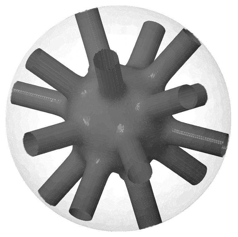
Figure 6. A surface inside a ball creating only two connected components in the interior and a large number of connected components on the boundary sphere.

In higher dimensions, the number of interior nodal domains does not control the number of boundary nodal domains (see Figure 6), and therefore new ideas are needed to tackle Open Problem 9. However, there are indications that a Courant-type (i.e. $O(n)$) bound should hold in this case as well. For instance, this is the case for cylinders and Euclidean balls (see Examples 1.3.2 and 1.3.3).

6.2. Geometry of the nodal sets

The nodal sets of Steklov eigenfunctions, both interior and boundary, remain largely unexplored. The basic property of the nodal sets of Laplace–Beltrami eigenfunctions is their density on the scale of $1/{\sqrt{\lambda}}$, where $\lambda$ is the eigenvalue (cf. [95], see also Figure 7). This means that for any manifold $\Omega$, there exists a constant $C$ such that for any eigenvalue $\lambda$ large enough, the corresponding eigenfunction $\phi_{\lambda}$ has a zero in any geodesic ball of radius $C/\sqrt{\lambda}$. This motivates the following questions (see also Figure 7):

Open Problem 10.

(i) Are the nodal sets of Steklov eigenfunctions on a Riemannian manifold $\Omega$ dense on the scale $1/\sigma$ in $\Omega$? (ii) Are the nodal sets of the Dirichlet-to-Neumann eigenfunctions dense on the scale $1/\sigma$ in $M=\partial\Omega$?

For smooth simply–connected planar domains, a positive answer to question (ii) follows from the work of Shamma [85] on asymptotic behaviour of Steklov eigenfunctions. On the other hand, the explicit representation of eigenfunctions on rectangles implies that there exist eigenfunctions of arbitrary high order which have zeros only on one pair of parallel sides. Therefore, a positive answer to (ii) may possibly hold only under some regularity assumptions on the boundary.

Figure 7. The nodal lines of the 30th eigenfunction on an ellipse.

Another fundamental problem in nodal geometry is to estimate the size of the nodal set. It was conjectured by S.-T. Yau that for any Riemannian manifold of dimension $n$,

$$C_{1}\sqrt{\lambda}\leq\mathcal{H}_{n-1}(\mathcal{N}(\phi_{\lambda}))\leq C_{2}\sqrt{\lambda},$$

where $\mathcal{H}_{n-1}(\mathcal{N}(\phi_{\lambda}))$ denotes the $n-1$-dimensional Hausdorff measure of the nodal set $\mathcal{N}(\phi_{\lambda})$ of a Laplace-Beltrami eigenfunction $\phi_{\lambda}$, and the constants $C_{1},C_{2}$ depend only on the geometry of the manifold. Similar questions can be asked in the Steklov setting:

Open Problem 11.

Let $\Omega$ be an $n$-dimensional Riemannian manifold with boundary $M$. Let $\phi_{\sigma}$ be an eigenfunction of the Steklov problem on $\Omega$ corresponding to the eigenvalue $\sigma$ and let $u_{\sigma}=\phi_{\sigma}|_{M}$ be the corresponding eigenfunction of the Dirichlet-to-Neumann operator on $M$. Show that

(i) $C_{1}\sigma\leq\mathcal{H}_{n-1}(\mathcal{N}(\phi_{\sigma}))\leq C_{2}\sigma,$

(ii) $C_{1}^{\prime}\sigma\leq\mathcal{H}_{n-2}(\mathcal{N}(u_{\sigma}))\leq C_{2}^{\prime}\sigma,$

where the constants $C_{1},C_{2},C_{1}^{\prime},C_{2}^{\prime}$ depend only on the manifold.

Some partial results on this problem are known. In particular, the upper bound in (ii) was conjectured by [8] and proved in [95] for real analytic manifolds with real analytic boundary. A lower bound on the size of the nodal set $\mathcal{N}(u_{\sigma})$ for smooth Riemannian manifolds (though weaker than the one conjectured in (ii) in dimensions $\geq 3$) was recently obtained in [92] using an adaptation of the approach of [87] to nonlocal operators.

The upper bound in (i) is related to the question of estimating the size of the zero set of a harmonic function in terms of its frequency (see [49]). In [82], this approach is combined with the methods of potential theory and complex analysis in order to obtain both upper and lower bounds in (i) for simply–connected analytic surfaces. Let us also note that the Steklov eigenfunctions decay rapidly away from the boundary [55], and therefore the problem of understanding the properties of the nodal set in the interior is somewhat analogous to the study of the zero sets of Schrödinger eigenfunctions in the “forbidden regions” (see [50]).

6.3. Multiplicity bounds for Steklov eigenvalues

In two dimensions, the estimate on the number of nodal domains allows to control the eigenvalue multiplicities (see [11, 17]). The argument roughly goes as follows: if the multiplicity of an eigenvalue is high, one can construct a corresponding eigenfunction with a high enough vanishing order at a certain point of a surface. In the neighbourhood of this point the eigenfunction looks like a harmonic polynomial, and therefore the vanishing order together with the topology of a surface yield a lower bound on the number of nodal domains. To avoid a contradiction with Courant’s theorem, one deduces a bound on the vanishing order, and hence on the multiplicity.

This general scheme was originally applied to Laplace-Beltrami eigenvalues, but it can be also adapted to prove multiplicity bounds for Steklov eigenvalues. Interestingly enough, one can obtain estimates of two kinds. Recall that the Euler characteristic $\chi$ of an orientable surface of genus $\gamma$ with $l$ boundary components equals $2-2\gamma-l$, and of a non-orientable one is equal to $2-\gamma-l$. Putting together the results of [63, 61, 59, 35] we get the following bounds:

Theorem 6.3.1.

Let $\Sigma$ be a compact surface of Euler characteristic $\chi$ with $l$ boundary components. Then the multiplicity $m_{k}(\Sigma)$ for any $k\geq 1$ satisfies the following inequalities:

(6.3.2) $$m_{k}(\Sigma)\leq 2k-2\chi-2l+5,$$

(6.3.3) $$m_{k}(\Sigma)\leq k-2\chi+3.$$

Note that the right-hand side of (6.3.2) depends only on the index of the eigenvalue $k$ and on the genus $\gamma$ of the surface, while the right-hand side of (6.3.3) depends also on the number of boundary components. Inequality (6.3.3) in this form was proved in [59]. In particular, it is sharp for the first eigenvalue of the disk ($\chi=2$, $l=1$, the maximal multiplicity is two) and of the Möbius band ($\chi=0$, $l=1$, the maximal multiplicity is four). Inequality 6.3.2 is sharp for the annulus ($\chi=0$, $l=2$, the maximal multiplicity is three and attained by the critical catenoid, see Theorem 4.3.4).

While these bounds are sharp in some cases, they are far from optimal for large $k$. In fact, the following result is an immediate corollary of Theorem 2.1.2.

Corollary 6.3.4.

[41] For any smooth compact Riemannian surface $\Omega$ with $l$ boundary components, there is a constant $N$ depending on the metric on $\Omega$ such that for $j>N$, the multiplicity of $\sigma_{j}$ is at most $2l$.

Remark 6.3.5.

The multiplicity of the first nonzero eigenvalue $\sigma_{1}$ has been linked to the relative chromatic number of the corresponding surface with boundary in [59].

For manifolds of dimension $n\geq 3$, no general multiplicity bounds for Steklov eigenvalues are available. Moreover, given a Riemannian manifold $\Omega$ of dimension $n\geq 3$ and any non-decreasing sequence of $N$ positive numbers, one can find a Riemannian metric $g$ in a given conformal class, such that this sequence coincides with the first $n$ nonzero Steklov eigenvalues of $(M,g)$ [60].

Theorem 6.3.6.

Let $\Omega$ be a compact manifold with boundary. Let $n$ be a positive integer and let $0=s_{0}<s_{1}\leq\cdots\leq s_{n}$ be a finite sequence. Then there exists a Riemannian metric $g$ on $\Omega$ such that $\sigma_{j}=s_{j}$ for $j=0,\cdots,n$.

For Laplace-Beltrami eigenvalues, a similar result was obtained in [21]. It is plausible that multiplicity bounds for Steklov eigenvalues in higher dimensions could be obtained under certain geometric assumptions, such as curvature constraints.

Acknowledgements

The authors would like to thank Brian Davies for inviting them to write this survey. The project started in 2012 at the conference on Geometric Aspects of Spectral Theory at the Mathematical Research Institute in Oberwolfach, and its hospitality is greatly appreciated. We are grateful to Mikhail Karpukhin and David Sher for helpful remarks on the preliminary version of the paper. We are also thankful to Dorin Bucur, Fedor Nazarov, Alexander Strohmaier and John Toth for useful discussions, as well as to Bartek Siudeja for letting us use his FEniCS eigenvalues computation code.

References

- [1] M. S. Agranovich. Some asymptotic formulas for elliptic pseudodifferential operators. Funktsional. Anal. i Prilozhen., 21(1):63–65, 1987.
- [2] M. S. Agranovich. On a mixed Poincaré-Steklov type spectral problem in a Lipschitz domain. Russ. J. Math. Phys., 13(3):239–244, 2006.
- [3] M. S. Agranovich and B. A. Amosov. Estimates for -numbers, and spectral asymptotics for integral operators of potential type on nonsmooth surfaces. Funktsional. Anal. i Prilozhen., 30(2):1–18, 96, 1996.
- [4] G. Alessandrini and R. Magnanini. Elliptic equations in divergence form, geometric critical points of solutions, and Stekloff eigenfunctions. SIAM J. Math. Anal., 25(5):1259–1268, 1994.
- [5] A. D. Alexandrov. Uniqueness theorems for surfaces in the large. I. Vestnik Leningrad. Univ., 11(19):5–17, 1956.
- [6] W. Arendt and R. Mazzeo. Friedlander’s eigenvalue inequalities and the Dirichlet-to-Neumann semigroup. Commun. Pure Appl. Anal., 11(6):2201–2212, 2012.
- [7] R. Bañuelos, T. Kulczycki, I. Polterovich, and B. Siudeja. Eigenvalue inequalities for mixed Steklov problems. In Operator theory and its applications, volume 231 of Amer. Math. Soc. Transl. Ser. 2, pages 19–34. Amer. Math. Soc., Providence, RI, 2010.
- [8] K. Bellova and F. Lin. Nodal sets of Steklov eigenfunctions. arXiv:1402.4323.
- [9] P. Bérard. Transplantation et isospectralité. I. Math. Ann., 292(3):547–559, 1992.
- [10] A. Besse. Manifolds all of whose geodesics are closed, volume 93 of Ergebnisse der Mathematik und ihrer Grenzgebiete [Results in Mathematics and Related Areas]. Springer-Verlag, Berlin-New York, 1978. With appendices by D. B. A. Epstein, J.-P. Bourguignon, L. Bérard-Bergery, M. Berger and J. L. Kazdan.
- [11] G. Besson. Sur la multiplicité de la première valeur propre des surfaces riemanniennes. Ann. Inst. Fourier (Grenoble), 30(1):x, 109–128, 1980.
- [12] R. Binoy and G. Santhanam. Sharp upper bound and a comparison theorem for the first nonzero steklov eigenvalue. Preprint arXiv:1208.1690v1, 2014.
- [13] L. Brasco, G. De Philippis, and B. Ruffini. Spectral optimization for the Stekloff-Laplacian: the stability issue. J. Funct. Anal., 262(11):4675–4710, 2012.
- [14] F. Brock. An isoperimetric inequality for eigenvalues of the Stekloff problem. Z. Angew. Math. Mech., 81(1):69–71, 2001.
- [15] P. Buser. Isospectral Riemann surfaces. Ann. Inst. Fourier (Grenoble), 36(2):167–192, 1986.
- [16] P. Buser, J. Conway, P. Doyle, and K.-D. Semmler. Some planar isospectral domains. Internat. Math. Res. Notices, (9):391ff., approx. 9 pp. (electronic), 1994.
- [17] S. Y. Cheng. Eigenfunctions and nodal sets. Comment. Math. Helv., 51(1):43–55, 1976.
- [18] B. Colbois, A. El Soufi, and A. Girouard. Isoperimetric control of the Steklov spectrum. J. Funct. Anal., 261(5):1384–1399, 2011.
- [19] B. Colbois and A. Girouard. The spectral gap of graphs and steklov eigenvalues on surfaces. Electron. Res. Announc. Math. Sci., 21:19–27, 2014.
- [20] B. Colbois and D. Maerten. Eigenvalues estimate for the Neumann problem of a bounded domain. J. Geom. Anal., 18(4):1022–1032, 2008.
- [21] Y. Colin de Verdière. Construction de laplaciens dont une partie finie du spectre est donnée. Ann. Sci. École Norm. Sup. (4), 20(4):599–615, 1987.
- [22] B. Dittmar. Sums of reciprocal Stekloff eigenvalues. Math. Nachr., 268:44–49, 2004.
- [23] P. Doyle and J. P. Rossetti. Laplace-isospectral hyperbolic 2-orbifolds are representation-equivalent. Preprint arXiv:1103.4372, 2014.
- [24] J. J. Duistermaat and V. W. Guillemin. The spectrum of positive elliptic operators and periodic bicharacteristics. Invent. Math., 29(1):39–79, 1975.
- [25] J. Edward. An inverse spectral result for the Neumann operator on planar domains. J. Funct. Anal., 111(2):312–322, 1993.
- [26] J. Edward. An inequality for Steklov eigenvalues for planar domains. Z. Angew. Math. Phys., 45(3):493–496, 1994.
- [27] A. El Soufi and S. Ilias. Riemannian manifolds admitting isometric immersions by their first eigenfunctions. Pacific J. Math., 195(1):91–99, 2000.
- [28] A. El Soufi and S. Ilias. Laplacian eigenvalue functionals and metric deformations on compact manifolds. J. Geom. Phys., 58(1):89–104, 2008.
- [29] J. F. Escobar. The geometry of the first non-zero Stekloff eigenvalue. J. Funct. Anal., 150(2):544–556, 1997.
- [30] J. F. Escobar. An isoperimetric inequality and the first Steklov eigenvalue. J. Funct. Anal., 165(1):101–116, 1999.
- [31] J. F. Escobar. A comparison theorem for the first non-zero Steklov eigenvalue. J. Funct. Anal., 178(1):143–155, 2000.
- [32] X.-Q. Fan, L.-F. Tam, and C. Yu. Steklov eigenvalues on annulus. Preprint arXiv:1310.7686.
- [33] D. W. Fox and J. R. Kuttler. Sloshing frequencies. Z. Angew. Math. Phys., 34(5):668–696, 1983.
- [34] A. Fraser and R. Schoen. The first Steklov eigenvalue, conformal geometry, and minimal surfaces. Adv. Math., 226(5):4011–4030, 2011.
- [35] A. Fraser and R. Schoen. Sharp eigenvalue bounds and minimal surfaces in the ball. Preprint arXiv:1209.3789, 2012.
- [36] A. Fraser and R. Schoen. Minimal surfaces and eigenvalue problems. In Geometric analysis, mathematical relativity, and nonlinear partial differential equations, volume 599 of Contemp. Math., pages 105–121. Amer. Math. Soc., Providence, RI, 2013.
- [37] A. Gabard. Sur la représentation conforme des surfaces de Riemann à bord et une caractérisation des courbes séparantes. Comment. Math. Helv., 81(4):945–964, 2006.
- [38] P. Gilkey. Asymptotic formulae in spectral geometry. Studies in Advanced Mathematics. Chapman & Hall/CRC, Boca Raton, FL, 2004.
- [39] P. Gilkey and G. Grubb. Logarithmic terms in asymptotic expansions of heat operator traces. Comm. Partial Differential Equations, 23(5-6):777–792, 1998.
- [40] A. Girouard, N. Nadirashvili, and I. Polterovich. Maximization of the second positive Neumann eigenvalue for planar domains. J. Differential Geom., 83(3):637–661, 2009.
- [41] A. Girouard, L. Parnovski, I. Polterovich, and D. Sher. The Steklov spectrum of surfaces: asymptotics and invariants. to appear in Math. Proc. Camb. Phil. Soc. Published online in August 2014.
- [42] A. Girouard and I. Polterovich. On the Hersch-Payne-Schiffer estimates for the eigenvalues of the Steklov problem. Funktsional. Anal. i Prilozhen., 44(2):33–47, 2010.
- [43] A. Girouard and I. Polterovich. Shape optimization for low Neumann and Steklov eigenvalues. Math. Methods Appl. Sci., 33(4):501–516, 2010.
- [44] A. Girouard and I. Polterovich. Upper bounds for Steklov eigenvalues on surfaces. Electron. Res. Announc. Math. Sci., 19:77–85, 2012.
- [45] C. Gordon, P. Herbrich, and D. Webb. Steklov isospectral manifolds. In preparation.
- [46] C. Gordon, P. Perry, and D. Schueth. Isospectral and isoscattering manifolds: a survey of techniques and examples. In Geometry, spectral theory, groups, and dynamics, volume 387 of Contemp. Math., pages 157–179. Amer. Math. Soc., Providence, RI, 2005.
- [47] A. Grigor’yan, Y. Netrusov, and S.-T. Yau. Eigenvalues of elliptic operators and geometric applications. In Surveys in differential geometry. Vol. IX, Surv. Differ. Geom., IX. Int. Press, Somerville, MA, 2004.
- [48] G. Grubb and R. Seeley. Weakly parametric pseudodifferential operators and Atiyah-Patodi-Singer boundary problems. Invent. Math., 121(3):481–529, 1995.
- [49] Q. Han and F.-H. Lin. On the geometric measure of nodal sets of solutions. J. Partial Differential Equations, 7(2):111–131, 1994.
- [50] B. Hanin, S. Zelditch, and P. Zhou. Nodal sets of random eigenfunctions for the isotropic harmonic oscillator. Int. Math. Res. Not. IMRN. To appear. Preprint: arXiv:1310.4532.
- [51] A. Hassannezhad. Conformal upper bounds for the eigenvalues of the Laplacian and Steklov problem. Journal of Functional Analysis, 261(12):3419–3436, 2011.
- [52] A. Henrot, G. Philippin, and A. Safoui. Some isoperimetric inequalities with application to the Stekloff problem. J. Convex Anal., 15(3):581–592, 2008.
- [53] J. Hersch. Quatre propriétés isopérimétriques de membranes sphériques homogènes. C. R. Acad. Sci. Paris Sér. A-B, 270:A1645–A1648, 1970.
- [54] J. Hersch, L. Payne, and M. Schiffer. Some inequalities for Stekloff eigenvalues. Arch. Rational Mech. Anal., 57:99–114, 1975.
- [55] P. D. Hislop and C. V. Lutzer. Spectral asymptotics of the Dirichlet-to-Neumann map on multiply connected domains in . Inverse Problems, 17(6):1717–1741, 2001.
- [56] L. Hörmander. The analysis of linear partial differential operators. IV, volume 275 of Grundlehren der Mathematischen Wissenschaften [Fundamental Principles of Mathematical Sciences]. Springer-Verlag, Berlin, 1985. Fourier integral operators.
- [57] S. Ilias and O. Makhoul. A Reilly inequality for the first Steklov eigenvalue. Differential Geom. Appl., 29(5):699–708, 2011.
- [58] D. Jakobson, M. Levitin, N. Nadirashvili, N. Nigam, and I. Polterovich. How large can the first eigenvalue be on a surface of genus two? Int. Math. Res. Not., 2005(63):3967–3985, 2005.
- [59] P. Jammes. Multiplicité du spectre de steklov sur les surfaces et nombre chromatique. arXiv:1304.4559.
- [60] P. Jammes. Une inégalité de Cheeger pour le spectre de Steklov. Preprint arXiv:1302.6540, 2013.
- [61] P. Jammes. Prescription du spectre de Steklov dans une classe conforme. Anal. PDE, 7(3):529–550, 2014.
- [62] A. Jollivet and V. Sharafutdinov. On an inverse problem for the Steklov spectrum of a Riemannian surface. In Inverse Problems and Applications, volume 615 of Contemporary Mathematics, pages v+235. American Mathematical Society, 2014.
- [63] M. Karpukhin, G. Kokarev, and I. Polterovich. Multiplicity bounds for Steklov eigenvalues on Riemannian surfaces. to appear in Ann. Inst. Fourier.
- [64] G. Kokarev. Variational aspects of Laplace eigenvalues on Riemannian surfaces. Preprint (2011): arXiv:1103.2448.
- [65] N. Korevaar. Upper bounds for eigenvalues of conformal metrics. J. Differential Geom., 37(1):73–93, 1993.
- [66] V. Kozlov and N. Kuznetsov. The ice-fishing problem: the fundamental sloshing frequency versus geometry of holes. Math. Methods Appl. Sci., 27(3):289–312, 2004.
- [67] J. R. Kuttler and V. G. Sigillito. Lower bounds for Stekloff and free membrane eigen-values. SIAM Rev., 10:368–370, 1968.
- [68] J. R. Kuttler and V. G. Sigillito. An inequality of a Stekloff eigenvalue by the method of defect. Proc. Amer. Math. Soc., 20:357–360, 1969.
- [69] N. Kuznetsov, T. Kulczycki, M. Kwaśnicki, A. Nazarov, S. Poborchi, I. Polterovich, and B. Siudeja. The legacy of Vladimir Andreevich Steklov. Notices Amer. Math. Soc., 61(1):9–22, 2014.
- [70] H. Lamb. Hydrodynamics. Cambridge University Press, 1879.
- [71] P. D. Lamberti and L. Provenzano. Viewing the Steklov eigenvalues of the laplace operator as critical neumann eigenvalues. Preprint.
- [72] J. Lee and G. Uhlmann. Determining anisotropic real-analytic conductivities by boundary measurements. Comm. Pure Appl. Math., 42(8):1097–1112, 1989.
- [73] P. Li and S. T. Yau. A new conformal invariant and its applications to the Willmore conjecture and the first eigenvalue of compact surfaces. Invent. Math., 69(2):269–291, 1982.
- [74] G. Liu. Heat invariants of the perturbed polyharmonic Steklov problem. arXiv:1405.3350.
- [75] A. Logg, K.-A. Mardal, and G. Wells, editors. Automated solution of differential equations by the finite element method, volume 84 of Lecture Notes in Computational Science and Engineering. Springer, Heidelberg, 2012. The FEniCS book.
- [76] N. Nadirashvili. Berger’s isoperimetric problem and minimal immersions of surfaces. Geom. Funct. Anal., 6(5):877–897, 1996.
- [77] J. Nečas. Direct methods in the theory of elliptic equations. Springer Monographs in Mathematics. Springer, Heidelberg, 2012. Translated from the 1967 French original by Gerard Tronel and Alois Kufner, Editorial coordination and preface by Šárka Nečasová and a contribution by Christian G. Simader.
- [78] O. Parzanchevski. On G-sets and isospectrality. Ann. Inst. Fourier (Grenoble), 63(6):2307–2329, 2013.
- [79] L. E. Payne. Some isoperimetric inequalities for harmonic functions. SIAM J. Math. Anal., 1:354–359, 1970.
- [80] R. Petrides. Existence and regularity of maximal metrics for the first laplace eigenvalue on surfaces. Geometric and Functional Analysis, pages 1–41, 2014.
- [81] I. Polterovich and D. Sher. Heat invariants of the Steklov problem. Journal of Geometric Analysis, to appear. Published online in September 2013.
- [82] I. Polterovich, D. Sher, and J. Toth. In preparation.
- [83] G. Rozenbljum. Asymptotic behavior of the eigenvalues for some two-dimensional spectral problems. In Selected translations, pages i–ii and 201–306. Birkhäuser Boston, Inc., Secaucus, NJ, 1986. Selecta Math. Soviet. 5 (1986), no. 3.
- [84] R. Schoen and S.-T. Yau. Lectures on differential geometry. Conference Proceedings and Lecture Notes in Geometry and Topology, I. International Press, Cambridge, MA, 1994.
- [85] S. E. Shamma. Asymptotic behavior of Stekloff eigenvalues and eigenfunctions. SIAM J. Appl. Math., 20:482–490, 1971.
- [86] B. Siudeja. Software webpage. http://pages.uoregon.edu/siudeja/software.php. Accessed: 2014-10-02.
- [87] C. D. Sogge and S. Zelditch. Lower bounds on the Hausdorff measure of nodal sets. Math. Res. Lett., 18(1):25–37, 2011.
- [88] T. Sunada. Riemannian coverings and isospectral manifolds. Ann. of Math. (2), 121(1):169–186, 1985.
- [89] G. Szegö. Inequalities for certain eigenvalues of a membrane of given area. J. Rational Mech. Anal., 3:343–356, 1954.
- [90] M. E. Taylor. Partial differential equations. II, volume 116 of Applied Mathematical Sciences. Springer-Verlag, New York, 1996.
- [91] G. Uhlmann. Inverse problems: seeing the unseen. Bull. Math. Sci., 4(2):209–279, 2014.
- [92] X. Wang and J. Zhu. A lower bound for the nodal sets of Steklov eigenfunctions. arXiv:1411.0708.
- [93] H. F. Weinberger. An isoperimetric inequality for the -dimensional free membrane problem. J. Rational Mech. Anal., 5:633–636, 1956.
- [94] R. Weinstock. Inequalities for a classical eigenvalue problem. J. Rational Mech. Anal., 3:745–753, 1954.
- [95] S. Zelditch. Measure of nodal sets of analytic Steklov eigenfunctions. arXiv:1403.0647.
- [96] S. Zelditch. Maximally degenerate Laplacians. Ann. Inst. Fourier (Grenoble), 46(2):547–587, 1996.