The Kolmogorov-Zakharov Model
for Optical Fiber Communication

Abstract

A mathematical framework is presented to study the evolution of multi-point cumulants in nonlinear dispersive partial differential equations with random input data, based on the theory of weak wave turbulence (WWT). This framework is used to explain how energy is distributed among Fourier modes in the nonlinear Schrödinger equation. This is achieved by considering interactions among four Fourier modes and studying the role of the resonant, non-resonant, and trivial quartets in the dynamics. As an application, a power spectral density is suggested for calculating the interference power in dense wavelength-division multiplexed optical systems, based on the kinetic equation of the WWT. This power spectrum, termed the Kolmogorov-Zakharov (KZ) model, results in a better estimate of the signal spectrum in optical fiber, compared with the so-called Gaussian noise (GN) model. The KZ model is generalized to non-stationary inputs and multi-span optical systems.

I Introduction

This paper studies the power spectral density (PSD) and the probability distribution of a signal propagating according to the one-dimensional cubic nonlinear Schrödinger (NLS) equation, which serves as a model for fiber-optic communication channels. A PSD known as the Gaussian noise (GN) model has been proposed for optical fiber communications [1, 2], resulting from a first-order perturbation approach to four-wave mixing in the NLS equation [1]. Although the GN model has appeared in the fiber-optic communications literature, there also exists a satisfactory and well-developed theory of the PSD for nonlinear dispersive equations in the context of wave turbulence in mathematical physics, and this theory forms the foundation for this paper.

From a mathematical point of view, the main idea of this approach to PSD can be broadly abstracted as follows. Suppose that a probability measure at the input $z=0$ of a partial differential equation (PDE) describing signal evolution in distance $z$ is given. We are interested in finding the probability measure at some $z>0$. First, all $n$-point moments of this probability distribution at $z=0$ are found. For reasons that are explained in Section VII-C, it is convenient to work with cumulants in place of moments, which are in one-to-one relation with one another. Then, a hierarchy of differential equations is obtained that governs the evolution of cumulants in distance. Under certain assumptions, this hierarchy is truncated at some order $n$, ignoring the influence of higher order cumulants. This turns the original infinite-dimensional functional problem into a finite-dimensional differential system for a set of scalar parameters, which is subsequently solved to obtain cumulants at distance $z>0$. Finally, cumulants at $z$ are combined to obtain the probability measure at $z$. The aim of wave turbulence theory is to study energy distribution in the frequency domain via the PSD, a 2-point cumulant. As a result, the emphasis is heavily placed on correlation function; nevertheless the idea is useful to obtain information on higher-order statistics.

In strong turbulence, encountered e.g., in the Navier-Stokes equations of hydrodynamics, nonlinearity can be strong and the cumulant hierarchy may not truncate. However in weak wave turbulence (WWT), under a weak nonlinearity assumption, which holds in optical fiber, the hierarchy is truncated and a differential equation for the PSD, known as a kinetic equation, is obtained. [3, 4, 5]. The kinetic equations of WWT can often be solved using, e.g., Zakharov conformal transformations to obtain Kolmogorov-Zakharov (KZ) stationary spectra. In this paper, we study 2-, 4- and 6-point cumulants, with the aim of obtaining a more accurate spectrum for interference and probability distribution than what is currently known in communications.

Turbulence theory helps us to understand the mechanisms by which the signal of one user is transported to the other users in a multiuser communication system. For instance, kinetic equations provide accurate predictions of interference power. More importantly, the theory gives useful insights into inter-channel interactions in wavelength-division multiplexing (WDM). WWT also yields a suitable mathematical framework for statistical signal analysis in optical fiber, which we use for modeling.

The contributions of the paper are organized as follows.

In Section III we describe the channel model. We focus on the frequency domain and introduce both a continuous and a discrete model, as it turns out there are differences among them.

In Section IV we derive the GN model in a simplified manner. We point out some of the shortcomings of the perturbation approach when applied to equations of type NLS.

To help understand interference, in Section V we describe energy transfer mechanisms in optical fiber via resonant manifolds and classification of quartets. We explain how energy transport differs between integrable and non-integrable channels.

We introduce the basic KZ model in Section VI and explain how it relates to the GN model. The standard kinetic equation of the WWT predicts a stationary spectrum for the integrable NLS equation. However, the analysis can be carried out to the next order in the nonlinearity level to account for deviations from the stationary spectrum. We compare the KZ and GN PSDs and show that the KZ PSD is equally simple yet provides better estimates of WDM interference. The KZ model describes energy fluxes correctly; for instance, unlike the GN model, the KZ spectrum of the lossless optical fiber is energy-preserving. The KZ model also predicts a quasi-Gaussian distribution, which is close to a Gaussian one. However, this small deviation from the Gaussian distribution, not captured by the GN model, is responsible for spectrum evolution and interference.

Sections VIII and IX are dedicated to further details about the KZ and GN models. The assumptions of the KZ model are examined in the context of communications. The KZ model is generalized to WDM and multi-span systems.

The power spectral density is a central object in statistical studies of nonlinear dispersive waves and is widely studied in mathematical physics. One aim of this paper is to point this out and show that some of the elaborate PSD calculations in communications engineering can be succinctly modified and methodically generalized in the more fundamental framework of WWT. The reader is referred to [3, 5] for an introduction to WWT and to [6, 7] for a survey of optical turbulence—mostly in higher-dimensional non-integrable models or in laser applications [6]. One-dimensional turbulence in integrable systems, which is the focus of this paper, is discussed in [4, 8].

II Notation and Preliminaries

The Fourier transform of $q(t)$ is represented as

$$\mathcal{F}(q)(\omega)\stackrel{{\scriptstyle\Delta}}{{=}}\int\limits_{-\infty}^{\infty}q(t)e^{j\omega t}\mathrm{d}t.$$ (1)

We use subscripts to denote the frequency variable, e.g., $q_{\omega}=\mathcal{F}(q)(\omega)$. Fourier series coefficients of a periodic signal $q(t)$ are similarly denoted by $q_{k}=\mathcal{F}_{s}(q)(k)$. When there are multiple frequencies $\omega_{i}$ in an expression, for brevity we often use shorthand notations $q_{i}\stackrel{{\scriptstyle\Delta}}{{=}}q(\omega_{i})$ and $\mathrm{d}\omega_{1\cdots n}\stackrel{{\scriptstyle\Delta}}{{=}}\prod_{i=1}^{n}\mathrm{d}\omega_{i}$. In such cases, it will be clear from the context whether $q_{i}$ corresponds to a discrete or a continuous frequency variable. To avoid confusion, we do not use subscripts to denote a time variable.

The following notation is used throughout the paper

$$\delta_{k_{1}\cdots k_{2n}}\stackrel{{\scriptstyle\Delta}}{{=}}\delta(s_{1}k_{1}+\cdots+s_{2n}k_{2n}),\quad k_{i}\in\mathbb{Z},$$

where $\delta(m)$ is the Kronecker delta and

$$s_{i}\stackrel{{\scriptstyle\Delta}}{{=}}\begin{cases}1,&1\leq i\leq n,\\ -1,&n+1\leq i\leq 2n.\end{cases}$$

For continuous frequencies, the corresponding real subscript $\omega_{1}\cdots\omega_{2n}$ is shortened to the integer subscript $1\cdots 2n$

$$\delta_{1\cdots 2n}\stackrel{{\scriptstyle\Delta}}{{=}}\delta(s_{1}\omega_{1}+\cdots+s_{2n}\omega_{2n}),\quad\omega_{i}\in\mathbb{R},$$ (2)

where, with notation abuse, $\delta(\omega)$ is the Dirac delta function.

Let $q(t)$ be a zero-mean stochastic process. The symmetric $2n$-point correlation functions in time (temporal moments) are

$$R(t_{1}\cdots t_{2n})\stackrel{{\scriptstyle\Delta}}{{=}}\mathsf{E}\Bigl{[}q(t_{1})\cdots q(t_{n})q^{*}(t_{n+1})\cdots q^{*}(t_{2n})\Bigr{]},$$ (3)

where $\mathsf{E}$ denotes expectation with respect to the corresponding joint probability distribution. Similarly, the $2n$-point spectral moments are

$$\mu_{1\cdots 2n}\stackrel{{\scriptstyle\Delta}}{{=}}\mathsf{E}\Bigl{[}q_{1}\cdots q_{n}q^{*}_{n+1}\cdots q^{*}_{2n}\Bigr{]}.$$ (4)

The asymmetric correlation functions and moments, in which the number of conjugate and non-conjugate variables is not the same, is assumed to be zero. If $n=1$, $\mu_{12}$ corresponds to the correlation between $q(\omega_{1})$ and $q(\omega_{2})$.

If a stochastic process $q(t)$ is (strongly) stationary, then

$$R(t_{1},\cdots,t_{2n})=R(t_{1}-t_{0},\cdots,t_{2n}-t_{0}),$$ (5)

for any reference point $t_{0}$ and $n\geq 1$. It is shown in Appendix A-A that if $q(t)$ is stationary, then

$$\mu_{1\cdots 2n}=S_{1\cdots 2n}\delta_{1\cdots 2n},$$ (6)

where

$$S_{1\cdots 2n} = \mathcal{F}(R(0,t_{2},\cdots,t_{2n}))(0,s_{2}\omega_{2},\cdots,s_{2n}\omega_{2n}),$$

is the moment density function. Thus $\mu_{1\cdots 2n}$ is non-zero only on the stationary manifold

$$s_{1}\omega_{1}+\cdots+s_{2n}\omega_{2n}=0.$$ (7)

If $n=1$, $\mu_{12}=S_{11}\delta_{12}$. We shorten equal indices as $S_{k}\stackrel{{\scriptstyle\Delta}}{{=}}S_{kk}$.

In addition to correlation functions and spectral moments, we also require spectral cumulants $\kappa_{1\cdots 2n}$ and their densities $\tilde{S}_{1\cdots 2n}$. The reader is referred to Appendix A-B for the definition of cumulants and their relation with moments. It is shown that the $2n$-point moments decompose in terms of the $2k$-point cumulants, $k\leq n$. Particularly, if $n=2,3$, from (74):

$$\mu_{1234} = S_{1234}\delta_{1234}$$ (8)

$$= S_{1}S_{2}\Bigl{(}\delta_{13}\delta_{24}+\delta_{14}\delta_{23}\Bigr{)}+\tilde{S}_{1234}\delta_{1234},$$

$$\mu_{123456} = S_{123456}\delta_{123456}$$ (9)

$$= S_{1}S_{2}S_{3}\Bigl{(}\delta_{14}\delta_{25}\delta_{36}+\delta_{14}\delta_{26}\delta_{35}$$

$$+\delta_{15}\delta_{24}\delta_{36}+\delta_{15}\delta_{26}\delta_{34}$$

$$+\delta_{16}\delta_{24}\delta_{35}+\delta_{16}\delta_{25}\delta_{34}\Bigr{)}+\tilde{S}_{123456}\delta_{123456},$$

where $\tilde{S}_{1234}$ and $\tilde{S}_{123456}$ are cumulant densities.

For a Gaussian distribution, only the mean and the 2-point cumulants are non-zero. Consequently, $\mu_{1\cdots 2n}$ is concentrated on normal manifolds

$$s_{l}\omega_{l}+s_{k}\omega_{k}=0,\quad 1\leq l\leq n,\quad n+1\leq k\leq 2n,$$

which are subsets of the stationary manifold. Other distributions generally have infinitely many non-zero cumulants. As a result, cumulants are used in this paper to measure deviations from the Gaussian distribution. A zero-mean distribution is defined to be quasi-Gaussian if

$$\tilde{S}_{1\cdots n}\approx 0,\quad\forall n\geq 6.$$ (10)

That is to say, at most 4-point cumulants are significant.

We will often make use of the trilinear integral and sum of the signals $q_{\omega}(z)$ and $q_{k}(z)$, defined as

$$\mathcal{N}_{\omega}(q,q,q)(z)\stackrel{{\scriptstyle\Delta}}{{=}}\int\limits_{-\infty}^{\infty}q_{1}(z)q_{2}(z)q^{*}_{3}(z)\delta_{123\omega}\mathrm{d}\omega_{123},$$ (11)

and

$$\mathcal{N}_{k}(q,q,q)(z)\stackrel{{\scriptstyle\Delta}}{{=}}\sum\limits_{lmn\>\in\>\textnormal{nr}_{k}}q_{\ell}(z)q_{m}(z)q_{n}^{*}(z),$$ (12)

where $\textnormal{nr}_{k}$ is the set of the non-resonant frequencies

$${\textnormal{nr}}_{k}\stackrel{{\scriptstyle\Delta}}{{=}}\Bigl{\{}(l,m,n)\>\bigl{|}\>l+m=n+k,\>l\neq k,\>m\neq k\Bigr{\}}.$$

These expressions help to factor out part of the complexity.

The following simple lemma is frequently used in Section IV when passing from the zero-order to the first-order in perturbation expansions.

Lemma 1.

Let $q_{\omega}(z)\stackrel{{\scriptstyle\Delta}}{{=}}\exp\left(j\omega^{2}z\right)q_{\omega}(0)$. Then

$$\int\limits_{0}^{z}e^{-jz^{\prime}\omega^{2}}\mathcal{N}_{\omega}(q,q,q)(z^{\prime})\mathrm{d}z^{\prime} =$$

$$j\int H_{123\omega}(z)q_{1}(0)q_{2}(0)q_{3}^{*}(0)\delta_{123\omega}\mathrm{d}\omega_{123\omega},$$

where the $H$-function is

$$H_{123\omega}(z)\stackrel{{\scriptstyle\Delta}}{{=}}\begin{cases}(1-e^{j\Omega_{123\omega}z})/\Omega_{123\omega},&\Omega_{123\omega}\neq 0,\\ -jz,&\Omega_{123\omega}=0,\end{cases}$$ (13)

in which

$$\Omega_{123\omega}\stackrel{{\scriptstyle\Delta}}{{=}}\omega_{1}^{2}+\omega_{2}^{2}-\omega_{3}^{2}-\omega^{2}.$$

Proof.

The result follows by substitution. ∎

Depending on the context, we may write the $H$-function as $H_{123\omega}$, $H_{123\omega}(z)$ or $H(\Omega_{123\omega})(z)$. A similar lemma can be stated for the trilinear sum (12).

III Channel Model

III-A Continuous-frequency NLS Equation

We consider the one-dimensional cubic dimensionless NLS equation on the real line

$$j\partial_{z}q=\partial_{tt}q+2|q|^{2}q,\quad(t,z)\in\mathbb{R}\times\mathbb{R}^{+},$$ (14)

where $q(t,z)$ is the signal as a function of space $z$ and time $t$. To focus on main ideas, in this section we consider only a single span lossless fiber. Loss and amplification in multi-span systems are introduced later in Section IX.

Using Duhamel’s formula, the differential equation (14) can be re-written as an integral equation

$$q_{\omega}(z) = e^{jz\omega^{2}}q_{\omega}(0)$$ (15)

$$-\>2j\int\limits_{0}^{z}e^{j(z-z^{\prime})\omega^{2}}\mathcal{N}_{\omega}(q,q,q)(z^{\prime})\mathrm{d}z^{\prime},$$

where $\mathcal{N}_{\omega}$, defined in (11), represents interaction among all four waves $123\omega$, and $\delta_{123\omega}$ denotes the corresponding frequency matching condition

$$\omega_{1}+\omega_{2}=\omega_{3}+\omega.$$ (16)

An interacting quartet can be shown schematically as $12\rightarrow 3\omega$.

Definition 1 (Trivial interactions).

A subset of frequencies in (16) are trivial interactions

$$\left(\omega_{1}=\omega_{3},\>\omega_{2}=\omega\right),\quad\left(\omega_{1}=\omega,\>\omega_{2}=\omega_{3}\right).$$ (17)

These frequencies form a set of zero Lebesgue measure on the hyperplane (16) and do not contribute to the integral (15) — unless the integrand has a delta function on (17); see (26). ∎

III-B Discrete-frequency NLS Equation

We also consider the NLS equation on torus $t\in\mathbb{T}=\mathbb{R}/(T\mathbb{Z})$, corresponding to $T$-periodic signals. Partitioning the sums

$$\sum\limits_{lm} = \sum\limits_{(l=k)\vee(m=k)}+\sum\limits_{(l\neq k)\wedge(m\neq k)},$$

$$\sum\limits_{(l=k)\vee(m=k)} = \sum\limits_{l=k}+\sum\limits_{m=k}-\sum\limits_{(l=k)\wedge(m=k)},$$ (18)

where $\vee$ and $\wedge$ are, respectively, or and and operations, we get the identity

$$\mathcal{F}_{s}(|q|^{2}q)(k)=2{\mathcal{P}}q_{k}-|q_{k}|^{2}q_{k}+\mathcal{N}_{k}(q,q,q)(z),$$ (19)

where ${\mathcal{P}}\stackrel{{\scriptstyle\Delta}}{{=}}\left\lVert q(t)\right\rVert_{2}^{2}/T$. The NLS equation in the discrete frequency domain is

$$\partial_{z}q_{k}=j\omega_{0}^{2}k^{2}q_{k}-\underbrace{4j{\mathcal{P}}q_{k}}_{\text{XPM}}+\underbrace{2j|q_{k}|^{2}q_{k}}_{\text{SPM}}-2j\underbrace{\mathcal{N}_{k}(q,q,q)(z)}_{\text{FWM}},$$ (20)

where SPM, XPM and FWM denote self-phase modulation, cross-phase modulation and four-wave mixing. Note that the SPM and XPM indices ($l=k$ or $m=k$) have been removed from $\mathcal{N}_{k}$. Unlike their continuous version (17), these indices form a set with non-zero measure and have no analogue in (15). Note further that the XPM is a constant phase shift, thanks to conservation of energy.

(a)	(b)
(c)	(d)

Figure 1: Interacting quartets. Here $(l,m)$ and conjugate variables $(n,k)$ are shown on two copies of the $x$-axis, placed on top of each other. A combined index like $nk$ means $n=k$. (a) Regular FWM $x_{l}x_{m}x_{n}^{*}$ ($l\neq m\neq n\neq k$), (b) two degenerate FWMs $x_{l}x_{m}x_{k}^{*}$ ($l\neq m\neq k$) and $x_{l}^{2}x_{n}^{*}$ ($l\neq n\neq k$), (c) two XPMs $|x_{l}|^{2}x_{k}$ and $|x_{m}|^{2}x_{k}$ ($l,m\neq k$) (d) SPM $|x_{k}|^{2}x_{k}$ ($l=m=n=k$).

As in the continuous model, the integral form of (20) is

$$q_{k}(z) = e^{j(\omega_{0}^{2}k^{2}-4{\mathcal{P}})z}\Bigl{\{}q_{k}(0)-2j\int_{0}^{z}e^{-j(\omega_{0}^{2}k^{2}-4{\mathcal{P}})z^{\prime}}$$ (21)

$$\>\times\Bigl{(}-|q_{k}(z^{\prime})|^{2}q_{k}(z^{\prime})+\mathcal{N}_{k}(q,q,q)(z^{\prime})\Bigr{)}\mathrm{d}z^{\prime}\Bigr{\}}.$$

Example 1 (Classification of quartets).

Consider the sum

$$S \stackrel{{\scriptstyle\Delta}}{{=}} \bigl{|}\left(x_{-2}+x_{-1}+x_{0}+x_{1}+x_{2}\right)\bigr{|}^{2}$$

$$\times\left(x_{-2}+x_{-1}+x_{0}+x_{1}+x_{2}\right).$$

The interference terms at frequency $k=0$ are ($l+m=n+0$)

$$S_{0} = |x_{0}|^{2}x_{0}+\underbrace{2x_{0}\left[|x_{-2}|^{2}+|x_{-1}|^{2}+|x_{1}|^{2}+|x_{2}|^{2}\right]}_{\text{degenerate quartet }(l=k)\vee(n=k)}$$ (22)

$$+\Bigl{\{}\underbrace{2x_{0}^{*}\bigl{(}x_{-2}x_{2}+x_{-1}x_{1}\bigr{)}}_{\text{degenerate FWM }n=k}+\underbrace{\bigl{(}x_{-1}^{2}x_{-2}^{*}+x_{1}^{2}x_{2}^{*}\bigr{)}}_{\text{degenerate FWM }l=m}$$

$$+\underbrace{2\bigl{(}x_{-2}x_{-1}^{*}x_{1}++x_{-1}x_{1}^{*}x_{2}\bigr{)}}_{\text{non-degenerate FWM }l\neq m\neq n\neq k}\Bigr{\}}.$$

There are several possibilities for a quartet $lm\rightarrow nk$. If all indices are different, we get non-degenerate FWM. If two indices of the same conjugacy type are equal, i.e., if $l=m$ or $n=k$, we obtain degenerate FWM. The cases that two indices of the opposite conjugacy type are the same, i.e., $l=k$ or $n=k$, are also degenerate quartets. These are the terms with the square brackets in (22). The literature refers to these terms as XPM, not degenerate FWM. The degenerate quartet with multiplicity two where $l=m=n=k$ is known as the SPM in the literature. However, according to our definition in (20), the SPM in (22) is $-|x_{0}|^{2}x_{0}$ and the XPM is the term with the square brackets plus $2|x_{0}|^{2}x_{0}$. This simplifies XPM to $2{\mathcal{P}}x_{0}$ and negates the sign of the SPM, as in (19)–(20). There are one SPM, ten XPM and ten FWM terms in this example. In general if $-N\leq k\leq N$, a simple counting shows that there are $3N^{2}+3N+2$ (XPM and FWM) interference terms at $k=0$. This number decreases as $k$ approaches the boundaries $\pm N$. The XPM, degenerate and non-degenerate FWM constitute, respectively, the 1-, 2- and 3-wave interference.

∎

IV GN Model

The GN “model” in the literature refers to a PSD. In this section, we re-derive this PSD for the continuous and discrete models in a simplified manner. This clarifies GN PSD, so that in Section VII it can be compared with the KZ PSD.

IV-A Continuous-frequency NLS Equation

Note that (15) is a fixed-point equation, mapping $q(z)$ to itself. Iterating the fixed-point map $q^{(k)}_{\omega}(z)\rightarrow q^{(k+1)}_{\omega}(z)$ starting from $q^{(-1)}_{\omega}=0$, we obtain

$$q_{\omega}^{(0)}(z)=e^{jz\omega^{2}}q_{\omega}(0).$$

This is just the solution of the linear part of the NLS equation. Iterating one more time and using Lemma 1, the signal to the first-order in nonlinearity level is

$$q_{\omega}^{(1)}(z) = e^{jz\omega^{2}}\Bigl{\{}q_{\omega}(0)$$ (23)

$$+\>2\int H(\Omega_{123\omega})(z)q_{1}(0)q_{2}(0)q_{3}^{*}(0)\delta_{123\omega}\mathrm{d}\omega_{123}\Bigr{\}},$$

where $H(\Omega_{123\omega})(z)$ is defined in (13).

It follows that the NLS equation has the simple closed-form solution (23) to the first-order in the perturbation expansion. As a consequence, derived quantities such as the PSD can also be calculated. Computing $\mu_{12}$ from (23) and removing factor $\delta_{12}$, we get

$$S_{\omega}(z) = S_{\omega}(0)+4\int\Re(H_{123\omega}S_{123\omega})\delta_{123\omega}\mathrm{d}\omega_{123}$$ (24)

$$+4\int H_{123\omega}H_{1^{\prime}2^{\prime}3^{\prime}\omega}^{*}S_{123^{\prime}1^{\prime}2^{\prime}3}\delta_{123\omega}\delta_{1^{\prime}2^{\prime}3^{\prime}\omega}\mathrm{d}\omega_{1231^{\prime}2^{\prime}3^{\prime}}.$$

Equation (24) expresses a 2-point PSD as a function of the 4- and 6-point PSDs. We can close the equation for the 2-point PSD if we assume that signal statistics are Gaussian. With this assumption, the 4- and 6-point PSDs break down according to (8)–(9), with zero cumulants. From (8)

$$S_{123\omega}\delta_{123\omega}=S_{1}S_{2}(\delta_{13}\delta_{2\omega}+\delta_{1\omega}\delta_{23}).$$ (25)

The right hand side in (25) is real and supported on trivial interactions (17), where $H_{123\omega}=-jz$. Thus $\Re(H_{123\omega}S_{123\omega})=0$ and the first integral in (24) vanishes.

For the second integral in (24), note that

$$S_{123^{\prime}1^{\prime}2^{\prime}3}\delta_{1^{\prime}2^{\prime}3^{\prime}\omega}\delta_{123\omega} = S_{123^{\prime}1^{\prime}2^{\prime}3}\delta_{123^{\prime}1^{\prime}2^{\prime}3}\delta_{123\omega}$$

$$= \mu_{123^{\prime}1^{\prime}2^{\prime}3}\delta_{123\omega}.$$

From (9)

$$\mu_{123^{\prime}1^{\prime}2^{\prime}3}=S_{1}S_{2}S_{3}\left(\delta_{11^{\prime}}\delta_{22^{\prime}}+\delta_{12^{\prime}}\delta_{21^{\prime}}\right)\delta_{33^{\prime}},$$ (26)

where the other four terms are ignored. They lead to secular terms; we will include them in Section IV-C, (33).

Integrating over primed variables, the resulting first-order PSD is

$$S_{\omega}^{\text{GN}}(z)=S_{\omega}^{0}+8\int|H_{123\omega}|^{2}S_{1}^{0}S_{2}^{0}S_{3}^{0}\delta_{123\omega}\mathrm{d}\omega_{123},$$ (27)

where $S_{\omega}^{0}\stackrel{{\scriptstyle\Delta}}{{=}}S_{\omega}(0)$ is the input PSD. This PSD is known as the GN model (PSD) in the literature [1, 2].

Note that, the signal energy is preserved in the NLS equation (14). However, the first-order signal (23) and its consequent PSD (27) are not energy preserving.

Remark 1.

Alternatively, the GN PSD can be obtained by simply approximating the nonlinear term $|q|^{2}q$ by $|q^{L}|^{2}q^{L}$ in the NLS equation,

$$j\partial_{z}q=q_{tt}+2|q|^{2}q\approx q_{tt}+2|q^{L}|^{2}q^{L},$$

where $q^{L}_{\omega}(z)\stackrel{{\scriptstyle\Delta}}{{=}}\exp(jz\omega^{2})q_{\omega}(0)$ is the solution of the linear part of the NLS equation.

∎

Remark 2.

In the NLS equation with physical parameters (59), the GN PSD (27) is of order $\gamma^{2}$, where $\gamma$ is the nonlinearity coefficient. If instead of $q^{(1)}(\omega)$, $q^{(2)}(\omega)$ is used in (24), additional terms are introduced to (27). One of these terms is of order $\mathcal{O}\left(\gamma^{2}\right)$, arising from the interaction of the linear term with a nonlinear quintic term in signal expansion. The GN PSD refers to the Fourier spectrum of the nonlinear term in (23), ignoring its interaction with other terms in the expansion of $q$.

∎

IV-B Discrete-frequency NLS Equation

As in the continuous-frequency model, we use the solution of the linear equation

$$q_{k}^{(0)}(z)=e^{j(\omega_{0}^{2}k^{2}-4{\mathcal{P}})z}q_{k}(0),$$ (28)

in (21) to obtain the first-order signal

$$q_{k}^{(1)}(z) = e^{j(\omega_{0}^{2}k^{2}-4{\mathcal{P}})z}\Bigl{(}q_{k}(0)+2jz|q_{k}(0)|^{2}q_{k}(0)$$ (29)

$$+2\sum\limits_{lmn\>\in\>\textnormal{nr}_{k}}H(\Omega_{lmnk})(z)q_{l}(0)q_{m}(0)q_{n}^{*}(0)\Bigr{)},$$

where

$$\Omega_{lmnk}\stackrel{{\scriptstyle\Delta}}{{=}}\omega_{0}^{2}(\ell^{2}+m^{2}-n^{2}-k^{2}).$$ (30)

Note that $\Omega_{lmnk}\neq 0$, since singularities $l=k$ and $m=k$ have been removed from $\mathcal{N}_{k}$.

Ignoring the SPM term $2jz|q_{k}(0)|^{2}q_{k}(0)$ in (29), squaring and averaging as before, the GN PSD is

$$S_{k}^{\text{GN}}(z)=S_{k}^{0}+8\sum\limits_{n}\sum\limits_{l\neq k}\sum\limits_{m\neq k}|H_{lmnk}|^{2}S_{l}^{0}S_{m}^{0}S_{n}^{0}\delta_{lmnk}.$$ (31)

The cross terms between linear and nonlinear parts in (29) is zero, similar to the continuous case.

IV-C Secular Behavior in the Signal Perturbation

It can be seen that the second term in (29), corresponding to SPM, grows unbounded with $z$. Had the XPM not been removed, that too would have produced a similar unbounded term. These degenerate FWM terms that tend to infinity with $z$ are called secular terms and make the series divergent. As a result, regular perturbation theory fails for the NLS equation.

The secular term of SPM can be removed using a multiple-scale analysis. For this purpose, we introduce an additional independent slow variable

$$\ell\stackrel{{\scriptstyle\Delta}}{{=}}\epsilon z,\quad q(t,z)\stackrel{{\scriptstyle\Delta}}{{=}}q(t,z,l),$$

where now $2\epsilon\ll 1$ is the nonlinearity coefficient. The NLS equation (20) is transformed to

$$\partial_{z}q_{k}+\epsilon\partial_{l}q_{k}=j\omega_{0}^{2}k^{2}q_{k}-2j\epsilon\left(2{\mathcal{P}}q_{k}-|q_{k}|^{2}q_{k}+\mathcal{N}_{k}\right).$$

We expand $q_{k}$ in powers of $\epsilon$ and equate powers of $\epsilon$ on both sides. We choose $\partial_{l}q_{k}=2j|q_{k}|^{2}q_{k}$ to remove the SPM singularity. Omitting details, the zero- and first-order terms (28) and (29) are, respectively, modified to

$$q_{k}^{(0)}(z) = e^{j(\omega_{0}^{2}k^{2}-4{\mathcal{P}}+2\epsilon|q_{k}(0)|^{2})z}q_{k}(0),$$

$$q_{k}^{(1)}(z) = e^{j\left(\omega_{0}^{2}k^{2}-4{\mathcal{P}}+2\epsilon|q_{k}(0)|^{2}\right)z}\Bigl{\{}q_{k}(0)$$ (32)

$$-\>2j\epsilon\sum\limits_{lmn\>\in\>\textnormal{nr}_{k}}H(\bar{\Omega}_{lmnk})q_{l}(0)q_{m}(0)q_{n}^{*}(0)\Bigr{\}},$$

where

$$\bar{\Omega} \stackrel{{\scriptstyle\Delta}}{{=}} \Omega_{lmnk}+j\omega_{0}^{2}\epsilon(|q_{l}(0)|^{2}+|q_{m}(0)|^{2}-|q_{n}(0)|^{2}-|q_{k}(0)|^{2}).$$

The PSD is given by (31) with $\Omega\rightarrow\bar{\Omega}$. It can be seen that the fast variable $z$ describes the rapid evolution of $q_{k}$ in small distance scales. However, as $z$ is increased, potentially important dynamics on large scales (where $\epsilon z\approx 1$) can be missed. In our example, the SPM term does indeed grow at scales of order $\mathcal{O}\left(\epsilon^{-1}\right)$. The role of the slow variable $l$ is to describe dynamics at this long-haul scale.

Secular terms seem to have been neglected in the literature. This is because missing the sum with minus sign in (18) ignores the SPM term in (20). However, typically energy is distributed over many Fourier modes and $z|q_{k}(z)|^{2}q_{k}(z)$ is quite small. As a result, if $z$ is not too large, the singular perturbation signal (29) is a good approximation and is simpler to use.

Secular terms appear in the continuous model too. Including the four terms missed in (26) gives the secular PSD contribution

$$S_{\omega}^{\textnormal{sec}} = 4\int H_{123\omega}H_{1^{\prime}2^{\prime}3^{\prime}\omega}^{*}\Bigl{\{}S_{1}S_{2}S_{3^{\prime}}\left(\delta_{1^{\prime}2}\delta_{2^{\prime}3^{\prime}}+\delta_{22^{\prime}}\delta_{1^{\prime}3^{\prime}}\right)\delta_{13}$$ (33)

$$+\>S_{1}S_{2}S_{3^{\prime}}\left(\delta_{11^{\prime}}\delta_{2^{\prime}3^{\prime}}+\delta_{12^{\prime}}\delta_{1^{\prime}3^{\prime}}\right)\delta_{23}\Bigr{\}}\delta_{123\omega}\mathrm{d}\omega_{1231^{\prime}2^{\prime}3^{\prime}}$$

$$= 16z^{2}{\mathcal{P}}^{2}S_{\omega}.$$

Figs. 2(a)–(b) demonstrate the accuracy of the first-order perturbation approximation (29). Here the strength of the nonlinearity is measured as the ratio $a(z)$ of the nonlinear and linear parts of the Hamiltonian [3]

$$\mathcal{H}(z)\stackrel{{\scriptstyle\Delta}}{{=}}j\int\limits_{-\infty}^{\infty}\biggl{(}\underbrace{\left|\partial_{t}q(t,z)\right|^{2}}_{\text{linear}}-\underbrace{\left|q(t,z)\right|^{4}}_{\text{nonlinear}}\biggr{)}\mathrm{d}t.$$

It can be seen in Figs. 2(a)–(b) that the perturbation series rapidly diverges as $A$ is increased. Even in the pseudo-linear regime where $a<0.1$, the error may not be small. Note that in the focusing regime, the linear and nonlinear parts of (23) add up destructively so that $\left\lVert q^{(1)}_{k}(z)\right\rVert<\left\lVert q_{k}(z)\right\rVert=\left\lVert q_{k}(0)\right\rVert$ and $q^{(1)}(t,1)$ is below $q(t,1)$ in Fig. 2(b). However, in the PSD the sign is lost and the linear and nonlinear PSDs add up constructively, so that $S_{k}(z)$ stands above $S_{k}^{0}$ in Fig. 5. As the amplitude is increased, the nonlinear term grows and, regardless of its angle, dominates the linear term. As a result, $q^{(1)}(t,z)$ goes above $q(t,z)$ and $\left\lVert q^{(1)}\right\rVert$ rapidly diverges to infinity. However, as we will see, the error in the PSD is typically smaller due to the squaring and averaging operations.

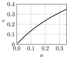
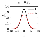
(a)	(b)

Figure 2: First-order signal approximation in perturbation expansion method when $q(t,0)=A\exp(-t^{2}/2)$ and $z=1$. (a) Error $e=\left\lVert q-q^{(1)}\right\rVert/\left\lVert q\right\rVert$ as a function of the nonlinearity parameter $a$. (b) Exact (E) and approximate (A) signals when $a=0.21$ ($A=0.5$).

V Energy Transfer in the Frequency Domain

In this section, we motivate the subsequent sections by explaining how energy is transferred among Fourier modes and why one might expect an asymptotically stationary PSD to the leading order in nonlinearity, when the signal propagates according to the NLS equation.

We begin with a two-dimensional Fourier series restricted on the dispersion relation $\zeta=\omega_{0}^{2}k^{2}$

$$q(t,z)=\sum\limits_{k=-\infty}^{\infty}a_{k}(z)e^{j(k\omega_{0}t+\omega_{0}^{2}k^{2}z)}.$$ (34)

Substituting (34) into the NLS equation, we get

$$\partial_{z}a_{k}(z)=-2j\sum\limits_{lmn}e^{j\Omega_{lmnk}z}a_{l}a_{m}a_{n}^{*}\delta_{lmnk},$$ (35)

where $\Omega_{lmnk}$ is defined in (30) and the sum is over all possible interactions $lm\rightarrow nk$. The integrating factor $\exp(j\omega_{0}^{2}k^{2}z)$ removes the additive dispersion term from the NLS equation and reveals it as an operator acting on nonlinearity in (35). If $\Omega_{lmnk}\neq 0$ and $z$ is large, the exponential term oscillates rapidly and the nonlinearity $a_{l}a_{m}a_{n}^{*}$ is averaged out in integration over $z$, following the Riemann-Lebesgue lemma. Therefore only modes lying on the resonant manifold

$$\ell+m=n+k,$$ (36a)

$$\smash{\left\{\IEEEstrut[8]\right.}$$ (37a)

$$\ell^{2}+m^{2}=n^{2}+k^{2},$$

contribute to the asymptotic changes in the Fourier mode $a_{k}$. This means that energy is transported in the frequency domain primary via the resonant interactions; the influence of the non-resonant interactions on energy transfer is small. The frequency and phase matching conditions (36a) and (37a) respectively represent conservation of the energy and momentum.

In our example, the resonant manifold (36a)–(37a) permits only trivial interactions

$$\{l=n,\>m=k\},\quad\text{or}\quad\{l=k,\>m=n\},$$ (38)

describing SPM ($\ell=m$) and XPM ($\ell\neq m$). Separating out the resonant indices from the sum in (35), we get

$$\partial_{z}a_{k}(z)=j(-4{\mathcal{P}}+2|a_{k}|^{2})a_{k}-2j\mathcal{N}^{\textnormal{nr}}_{k}(a,a,a),$$ (39)

where

$$\mathcal{N}^{\textnormal{nr}}_{k}(a,a,a)\stackrel{{\scriptstyle\Delta}}{{=}}\sum\limits_{lmn\>\in\>\textnormal{nr}_{k}}e^{j\Omega_{lmnk}z}a_{l}a_{m}a_{n}^{*}\delta_{lmnk},$$

contains only non-resonant quartets (the complement of the set (38)). Non-resonant interactions constitute the majority of all interactions, and since $\mathcal{N}^{\textnormal{nr}}_{k}\approx 0$, we observe that, when viewed in the four dimensional space $(l,m,n,k)$, most of the possible interactions are nearly absent.

Ignoring $N^{\textnormal{nr}}_{k}$ in (39), we obtain

$$a_{k}(z)\approx j(-4{\mathcal{P}}+2|a_{k}|^{2})a_{k},$$ (40)

which does not imply any inter-modal interactions. In fact, restoring the dispersion, we have

$$q_{k}(z)\approx e^{j\left(\omega_{0}^{2}k^{2}-4{\mathcal{P}}+2|q_{k}(0)|^{2}\right)z}q_{k}(0),$$

which means $|q_{k}(z)|\approx|q_{k}(0)|$. This is because the resonant quartets for the convex dispersion relation $\zeta=\omega^{2}$, $\omega=\omega_{0}k$, of the integrable NLS equation consists of only trivial quartets (38).

It follows that the signal spectrum is almost stationary. There are small oscillations in the spectrum due to small non-resonant effects, but because most of the possible interactions between Fourier modes, responsible for spectral broadening, do not occur, a localized energy stays localized and does not spread to infinite frequencies. This also intuitively explains the lack of the equipartition, and the periodic exchange, of the energy among Fourier modes in the Fermi-Pasta-Ulm (FPU) lattice [9] — and generally in soliton systems.

Fig. 3 shows the evolution of modes $k=0$ and $k=N/2$, where $N$ is the integer bandwidth, for input signal $q(t,0)=2\exp(-t^{2}/2)$ ($a(0)=5.65$) in the deterministic NLS equation. Despite local changes in distance, globally the signal spectrum is not broadened monotonically, but rather oscillates. Here evolution is continued for a very long distance $z=50$ (about $10^{5}$ km in a standard optical system). This is not surprising given that the orbits of integrable Hamiltonian systems in the phase space are periodic, confined to a torus. Sufficient perturbations to integrability break the characteristic oscillations in Fig. 3, though for small perturbations the oscillations persist. Note that if the input is a stochastic process and, instead of $|q_{k}(z)|$, the PSD $\mathsf{E}|q_{k}(z)|^{2}$ is plotted, these local oscillations are further averaged out so that the PSD is asymptotically almost stationary.

The steady-state stationary PSD, without much transient spectral broadening, is a consequence of integrability. Consider a non-integrable equation, e.g., by introducing a third-order dispersion to the NLS equation with dispersion relation $\zeta=\omega^{3}+3\omega^{2}$, $\omega=\omega_{0}k$. The resonant manifold is

$$\ell+m=n+k,$$ (41a)

$$\smash{\left\{\IEEEstrut[8]\right.}$$ (42a)

$$\ell^{3}+m^{3}+3(\ell^{2}+m^{2})=n^{3}+k^{3}+3(n^{2}+k^{2}).$$

Since the dispersion relation $\zeta=\omega^{3}+3\omega^{2}$ is non-convex, the resonant manifold contains a larger number of quartets than the trivial ones in (38), e.g., $(l,m,n,k)=(1,-3,0,-2)$. It can be verified that non-trivial quartets are

$$l+m=-2,\quad n+k=-2.$$

As before, ignoring $\mathcal{N}^{\textnormal{nr}}_{k}$, equation (40) now reads

$$a_{k}(z)\approx j(-4{\mathcal{P}}+2|a_{k}|^{2})a_{k}-2j\sum\limits_{\textnormal{nt}}a_{l}a_{m}a_{n}^{*},$$

where the sum is over non-trivial quartets, i.e., the resonant quartets in (41a)–(42a) excluding the trivial ones (38). The coupling introduced by non-trivial interactions creates a strong energy transfer mechanism, causing substantial spectral broadening (or narrowing, depending on the equation) and dispersing a localized energy to higher (lower) frequencies. Unlike the FPU lattice where energy is exchanged periodically among a few Fourier modes, energy partitioning continues until an equilibrium is reached. This can be a flat (equipartition) or non-flat stationary steady-state PSD, depending on the equation.

Note that if pulses have short duration, then $\omega_{0}\gg 1$ and the dispersion operator inside the sum in $\mathcal{N}^{\textnormal{nr}}_{k}$ averages out nonlinearity more effectively. This explains pseudo-linear transmission in the wideband regime.

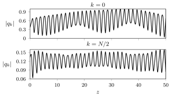
Figure 3: Evolution of two Fourier modes in distance.

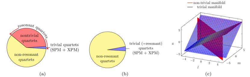
Figure 4: (a) Classification of quartets in a general nonlinear dispersive equation. When viewed in the four dimensional space $(l,m,n,k)$, many quartets do not (or weakly) interact. Transfer of energy occurs primarily among the resonant quartets. (b) In the integrable NLS equation, the dispersion relation is convex, as a result, the resonant quartets include only trivial quartets, which are quite sparse in the whole space. In addition, in energy-preserving NLS equation, trivial quartets do not interact. Only weak interactions due to non-resonant quartets are left. (c) Resonant manifold for dispersion relation $k=\zeta^{3}+3\zeta^{2}$. Energy flows on the red plane $l+m+2=0$. The two blue planes $n=l$ and $n=m$ form the trivial manifold. No energy flows on the blue planes.

To summarize, one can divide four-wave interactions into resonant and non-resonant interactions. Transfer of energy takes place primarily among the resonant modes and via the resonance mechanism. The resonant quartets are themselves divided into trivial and non-trivial quartets. Trivial quartets represent SPM and XPM and, in the energy-preserving integrable NLS equation, do not cause interaction. Non-trivial interactions, which are absent in the integrable equation, cause coupling and transfer of energy among all resonant modes. This occurs when higher order dispersion or nonlinear terms are introduced in the integrable NLS equation. The redistribution of energy among Fourier modes continues until an equilibrium (which is generally not an equipartition) is reached after a transient evolution. See Fig. 4.

VI The KZ Model Power Spectral Density

In this Section, we obtain the basic KZ PSD, in a single-channel single-span optical fiber with no loss and higher-order dispersion terms.

VI-A Kinetic Equation of the PSD

We assume that the signal is strongly stationary so that (5) holds. In particular

$$R(t_{1},t_{2};z)=R(\tau;z),\quad\tau\stackrel{{\scriptstyle\Delta}}{{=}}t_{2}-t_{1}.$$

As shown in Appendix A-A, stationarity implies that the signal is uncorrelated in the frequency domain

$$\mu_{12}(z)=S_{k}(z)\delta_{12},$$ (43)

where $S_{k}(z)=\mathcal{F}_{s}(R(\tau;z))(k)$.

Often the phase of a signal in a nonlinear dispersive equation varies rapidly compared to the slowly-varying amplitude. Furthermore, in some applications such as ocean waves, it is natural to assume that the initial data is random. This suggests a statistical approach, such as that in the turbulence theory. Here the evolution of the $n$-point spectral cumulants is described.

The NLS equation (14) consists of a linear term involving $q$ and a nonlinear term $|q|^{2}q$. As a result, the evolution of the $2$-point moment is tied to the $4$-point moment, the evolution of the $4$-point moment is tied to the $6$-point moment, and so on. For reasons explained in Section VII-C, we work with cumulants. Multivariate moments and cumulants are interchangeable via (73) and (75) in Appendix A-B. As a result, one obtains recursive differential equations for $2n$-point cumulants, each equation depending on cumulants up to $(2n+2)$-point. In strongly nonlinear systems, higher order cumulants are not negligible and the hierarchy of cumulant equations does not truncate. This makes strong turbulence, traditionally encountered in solid-state physics and fluid dynamics, a difficult problem. However, in weakly nonlinear systems, statistics are close to Gaussian and consequently higher-order cumulants can be neglected. As a result, a closure of the hierarchy of the cumulant equations is reached. This gives rise to a kinetic equation for the PSD. In WWT, kinetic equations can often be solved using, e.g., Zakharov conformal transformations. The resulting solutions are known as Kolmogorov-Zakharov spectra.

For non-integrable equations, kinetic equations indicate a monotonic transfer of energy to higher or lower frequencies (direct and reverse energy cascade) in the first order in nonlinearity. However, for integrable equations, kinetic equations immediately predict a stationary PSD to the first order. Nevertheless, for the NLS equation, the kinetic equation can be solved to the second order in the nonlinearity to account for changes in the PSD that are observed in numerical and experimental studies of the integrable NLS equation.

A differential equation for the 2-point moment $\mu_{kk}\stackrel{{\scriptstyle\Delta}}{{=}}S_{k}$ can be obtained straightforwardly:

$$\frac{\mathrm{d}S_{k}}{\mathrm{d}z} = \mathsf{E}\left\{q_{k}^{*}\partial_{z}q_{k}+\mathrm{c.c.}\right\}$$ (44)

$$= \mathsf{E}\Bigl{\{}q_{k}^{*}\bigl{(}j\omega_{0}^{2}k^{2}q_{k}-2j\sum q_{l}q_{m}q_{n}^{*}\delta_{lmnk}\bigr{)}+\mathrm{c.c.}\Bigr{\}}$$

$$= j\omega_{0}^{2}k^{2}S_{k}-2j\sum\mu_{lmnk}\delta_{lmnk}+\mathrm{c.c.}$$

$$= 4\sum\Im(\mu_{lmnk})\delta_{lmnk},$$

where $\mathrm{c.c.}$ stands for complex conjugate. To the zero order in the nonlinearity, the signal distribution is Gaussian and $\tilde{S}_{lmnk}=0$. As a result, $\Im(\mu_{lmnk})=0$ and $\mathrm{d}S_{k}/\mathrm{d}z=0$.

In the first order in the nonlinearity, the evolution of the 4-point moment is

$$\frac{\mathrm{d}\mu_{lmnk}}{\mathrm{d}z} = \mathsf{E}\bigl{\{}(\partial_{z}q_{l})q_{m}q_{n}^{*}q_{k}^{*}\bigr{\}}+\cdots$$ (45)

$$= \mathsf{E}\Bigl{\{}\Bigl{(}j\omega_{0}^{2}l^{2}q_{l}-2j\sum\limits_{l^{\prime}m^{\prime}n^{\prime}}q_{l^{\prime}}q_{m^{\prime}}q_{n^{\prime}}^{*}\delta_{l^{\prime}m^{\prime}n^{\prime}l}\Bigr{)}q_{m}q_{n}^{*}q_{k}^{*}\Bigr{\}}$$

$$+\>\cdots$$

$$= j\Omega_{lmnk}\mu_{lmnk}-2j\sum\limits_{l^{\prime}m^{\prime}n^{\prime}}\Bigl{\{}\mu_{l^{\prime}mm^{\prime}nn^{\prime}k}\delta_{l^{\prime}m^{\prime}n^{\prime}l}$$

$$\>+\mu_{ll^{\prime}m^{\prime}nn^{\prime}k}\delta_{l^{\prime}m^{\prime}n^{\prime}m}-\mu_{lmn^{\prime}l^{\prime}m^{\prime}k}\delta_{l^{\prime}m^{\prime}n^{\prime}n}$$

$$\>-\mu_{lmn^{\prime}l^{\prime}m^{\prime}n}\delta_{l^{\prime}m^{\prime}n^{\prime}k}\Bigr{\}}.$$

In the discrete model, dispersion is a multiplication by a unitary matrix. The linear and nonlinear parts of the NLS dynamics are mixing processes in time and frequency. When the input signal is quasi-Gaussian and signal phase is uniformly distributed in $z$, these mixing processes maintain the quasi-Gaussian distribution, in the view of the central limit theorem. As long as the signal phase is uniform and nonlinear interactions are weak, this is an excellent approximation.

It follows that, under the assumption that there are a large number of Fourier modes in weak interaction, and that the distribution of $q_{k}(0)$ is quasi-Gaussian, we can assume that the distribution of $q_{k}(z)$ remains quasi-Gaussian, as defined in (10). Consequently, the four 6-point moments in (45) break down in terms of the 2-point moments

$$\mu_{l^{\prime}mm^{\prime}nn^{\prime}k} = S_{m}S_{n}S_{k}\left(\delta_{mn^{\prime}}\delta_{l^{\prime}n}\delta_{m^{\prime}k}+\delta_{mn^{\prime}}\delta_{l^{\prime}k}\delta_{nm^{\prime}}\right)$$

$$\>+S_{m}S_{n}S_{n^{\prime}}\left(\delta_{mk}\delta_{\ell^{\prime}n}\delta_{m^{\prime}n^{\prime}}+\delta_{mk}\delta_{\ell^{\prime}n^{\prime}}\delta_{m^{\prime}n}\right)$$

$$\>+S_{m}S_{n^{\prime}}S_{k}\left(\delta_{mn}\delta_{\ell^{\prime}n^{\prime}}\delta_{m^{\prime}k}+\delta_{mn}\delta_{\ell^{\prime}k}\delta_{m^{\prime}n^{\prime}}\right),$$

$$\mu_{l^{\prime}m^{\prime}lnn^{\prime}k} = S_{l}S_{n}S_{k}\left(\delta_{ln^{\prime}}\delta_{l^{\prime}n}\delta_{m^{\prime}k}+\delta_{ln^{\prime}}\delta_{l^{\prime}k}\delta_{nm^{\prime}}\right)$$

$$\>+S_{\ell^{\prime}}S_{n}S_{k}\left(\delta_{l^{\prime}n^{\prime}}\delta_{m^{\prime}n}\delta_{\ell k}+\delta_{l^{\prime}n^{\prime}}\delta_{m^{\prime}k}\delta_{\ell n}\right)$$

$$\>+S_{m^{\prime}}S_{n}S_{k}\left(\delta_{m^{\prime}n^{\prime}}\delta_{\ell n}\delta_{\ell^{\prime}k}+\delta_{m^{\prime}n^{\prime}}\delta_{\ell k}\delta_{\ell^{\prime}n}\right),$$

$$\mu_{lmn^{\prime}l^{\prime}m^{\prime}k} = S_{l}S_{m}S_{k}\left(\delta_{n^{\prime}k}\delta_{ll^{\prime}}\delta_{mm^{\prime}}+\delta_{n^{\prime}k}\delta_{lm^{\prime}}\delta_{ml^{\prime}}\right)$$

$$+\>S_{l}S_{m}S_{n^{\prime}}\left(\delta_{n^{\prime}\ell^{\prime}}\delta_{\ell m^{\prime}}\delta_{mk}+\delta_{n^{\prime}\ell^{\prime}}\delta_{lk}\delta_{mm^{\prime}}\right)$$

$$+\>S_{k}S_{\ell^{\prime}}S_{n^{\prime}}\left(\delta_{n^{\prime}m^{\prime}}\delta_{\ell\ell^{\prime}}\delta_{mk}+\delta_{n^{\prime}m^{\prime}}\delta_{lk}\delta_{m\ell^{\prime}}\right),$$

$$\mu_{lmn^{\prime}l^{\prime}m^{\prime}n} = S_{l}S_{m}S_{n}\left(\delta_{n^{\prime}n}\delta_{ll^{\prime}}\delta_{mm^{\prime}}+\delta_{n^{\prime}n}\delta_{lm^{\prime}}\delta_{ml^{\prime}}\right)$$

$$\>+S_{l}S_{m}S_{n^{\prime}}\left(\delta_{n^{\prime}\ell^{\prime}}\delta_{\ell m^{\prime}}\delta_{mn}+\delta_{n^{\prime}\ell^{\prime}}\delta_{\ell n}\delta_{mm^{\prime}}\right)$$

$$\>+S_{l}S_{m}S_{n^{\prime}}\left(\delta_{m^{\prime}n^{\prime}}\delta_{\ell\ell^{\prime}}\delta_{mn}+\delta_{m^{\prime}n^{\prime}}\delta_{\ell n}\delta_{mn^{\prime}}\right).$$

Summing over primed variables in (45), the first two terms in the four expressions above add up to $4jT_{lmnk}\delta_{lmnk}$, where

$$T_{lmnk}(S,S,S)(z) \stackrel{{\scriptstyle\Delta}}{{=}} S_{l}S_{m}S_{n}+S_{l}S_{m}S_{k}$$

$$-\>S_{l}S_{n}S_{k}-S_{m}S_{n}S_{k}$$

is the collision term. The last four terms in the four expressions simplify to zero in (45). Canceling $\delta_{lmnk}$ in the resulting equation, it follows that

$$\frac{\mathrm{d}S_{lmnk}}{\mathrm{d}z} = j\Omega_{lmnk}S_{lmnk}+4jT_{lmnk}(S,S,S)(z),$$ (46)

where, recall that $\mu_{lmnk}=S_{lmnk}\delta_{lmnk}$.

In the standard WTT approach, it is assumed that $S_{lmnk}$ varies slowly. As a result, $\mathrm{d}S_{lmnk}/\mathrm{d}z\approx 0$ in (46), thus $S_{lmnk}=-4T_{lmnk}/\Omega_{lmnk}$. If $\Omega_{lmnk}=0$, $S_{lmnk}$ can not be determined from (46). Replacing $\Omega_{lmnk}$ with $\Omega_{lmnk}-j\epsilon$ and using the Kramers-Kronig relations [10, Lemma 1], we get $\Im(\frac{1}{x-j\epsilon})=-\pi\delta(x)$ in the sense of distributions. This gives $\Im(S_{lmnk})=4\pi T_{lmnk}/\Omega_{lmnk}\delta(\Omega_{lmnk})$ and, subsequently, the standard kinetic equation for the NLS equation

$$\frac{\mathrm{d}S_{k}}{\mathrm{d}z}=16\pi\sum\frac{T_{lmnk}}{\Omega_{lmnk}}\delta(\Omega_{lmnk})\delta_{lmnk}.$$

The product of the two delta functions dictates resonant (trivial) interactions (38). This means energy transfer occurs primarily among resonant modes. However, for resonant interactions $T_{lmnk}=0$, and a stationary spectrum is obtained. The stationarity of the turbulence spectrum of integrable systems is discussed in [4].

However, it can be seen in (46) that even if $T_{lmnk}$ is slowly varying, e.g., $T_{lmnk}=0$, $S_{lmnk}$ oscillates with spatial frequency $\Omega_{lmnk}$ for non-resonant quartets, for which $\Omega_{lmnk}\neq 0$. This linear dynamics modulates the collision term in (46). Since we are interested in non-stationary spectrum, we cannot assume $\mathrm{d}S_{lmnk}/\mathrm{d}z\approx 0$, and evolution of $S_{lmnk}$, due to non-resonant interactions, has to be accounted for in the next order. This is very easy to perform and has been pointed out in [8] as well.

The integral form of (46) is

$$S_{lmnk}(z) = e^{j\Omega_{lmnk}z}S_{lmnk}(0)$$ (47)

$$+\>4j\int\limits_{0}^{z}e^{j\Omega_{lmnk}(z-z^{\prime})}T_{lmnk}(S,S,S)(z^{\prime})\mathrm{d}z^{\prime}.$$

Since resonant interactions (38) do not contribute to $\mathrm{d}S_{k}/\mathrm{d}z$, below we include only non-resonant interactions for which $\Omega_{lmnk}\neq 0$ and $S_{lmnk}(0)=\tilde{S}_{lmnk}(0)$. Substituting (47) into (44), we obtain the kinetic equation for $S_{k}$

$$\frac{\mathrm{d}S_{k}}{\mathrm{d}z} = 4\sum\limits_{lmn\>\in\>\textnormal{nr}_{k}}\Im\left(e^{j\Omega_{lmnk}z}\tilde{S}_{lmnk}(0)\right)$$ (48)

$$+\>16\epsilon^{2}\sum\limits_{lmn\>\in\>\textnormal{nr}_{k}}\int_{0}^{z}\cos(\Omega_{lmnk}(z-z^{\prime}))T_{lmnk}(z^{\prime})\mathrm{d}z^{\prime},$$

where parameter $\epsilon$ is introduced to use it below.

The kinetic equation (48) is a nonlinear cubic equation similar to the NLS equations. However, now the rapidly-varying variables are averaged out and the PSD evolves very slowly so that the perturbation theory is better applicable. We thus solve (48) perturbatively, writing

$$S_{k}(z) = S_{k}^{(0)}(z)+\epsilon S_{k}^{(1)}(z)+\cdots,$$

$$S_{lmnk}(z) = S_{lmnk}^{(0)}(z)+\epsilon S_{lmnk}^{(1)}(z)+\cdots.$$

For the zero-order term we obtain

$$S_{k}^{(0)}(z)=S_{k}^{0}+4\Re\Bigl{(}\sum\limits_{lmn\>\in\>\textnormal{nr}_{k}}H_{lmnk}\tilde{S}_{lmnk}(0)\Bigr{)}.$$

If the input signal is quasi-Gaussian, $\tilde{S}_{lmnk}(0)\approx 0$ and the contribution of the second term to the PSD can be typically ignored. Consequently, we can substitute $S_{k}^{(0)}(z)=S_{k}^{0}$ in the equation of the next order. Omitting details, we obtain

$$S_{k}^{\text{KZ}}(z)=S_{k}^{0} + 8\epsilon^{2}\sum\limits_{\begin{subarray}{c}l\neq k\\ m\neq k\end{subarray}}|H_{lmnk}(z)|^{2}T_{lmnk}^{0}\delta_{lmnk}.$$ (49)

Note that if $z\rightarrow\infty$, $S_{k}^{\text{KZ}}$ is approximately stationary. Equation (49) is the KZ PSD.

VI-B KZ Model Assumptions

In this subsection, we summarize the assumptions of the KZ model and comment on their validity in the context of fiber-optic data communications.

Fourier transforms $q_{k}$ and $S_{k}$ exist

Particularly, $R(\tau;0)$ should vanish as $|\tau|\rightarrow\infty$.

This assumption is valid in data communications because signals have finite energy and time duration.

The input signal is strongly stationary

This ensures that the $2n$-point moments are concentrated on stationary manifolds. In particular, $q_{k}$ are uncorrelated, as stated in (43). The delta functions that follow from this assumption simplify the collision term in (45).

This assumption is valid in uncoded OFDM systems, where sub-carrier symbols are independent and the transmitted signal is cyclostationary. However, in coarse WDM systems the time-domain pulse shape can make the transmitted signal non-stationary and cause correlations in the frequency domain.

Signal has quasi-Gaussian distribution for all $z$ in the sense of (10)

In particular the input signal must be quasi-Gaussian. Under random phase approximation [3], the flow of the NLS equation would then ensure that the signal remains quasi-Gaussian in the weak nonlinearity framework. This assumption is needed in (8)–(9) to close the cumulant equations.

The integrable NLS equation in the focusing regime has stable soliton solutions. As pointed out in [5], the solitonic regime, in which the nonlinearity is strong, can act against the dispersive mixing of the weak nonlinearity regime. We assume that for random input the coherence is not developed. This means that the interference spectrum in the focusing and defocusing regimes are the same.

To summarize, Assumptions b) and c) may fail in data communications. However, the WWT approach can be re-worked out without using these assumptions. The price to pay is that the closure is achieved at orders above six (see (8)–(9)) and the expressions are not as simple. In Section VIII, we obtain the KZ spectrum for a WDM input signal with and without Assumptions b) and c).

VII Comparing the KZ and GN Models

In this section we explain how the KZ model differs from the GN model.

VII-A Differences in Assumptions

The GN model assumes a perfectly Gaussian distribution compared with the less stringent quasi-Gaussian assumption of the KZ model. Note that in the presence of the four-wave interactions $lm\rightarrow nk$, higher order moments are encountered. If a closure is to be reached, any perturbative method requires reducing high-order moments to low-order ones, i.e., the quasi-Gaussian assumption at some order. For example, the breakdown of the 6-point moments is also required in the GN model, in closing (24) for the 2-point moment.

The GN PSD in some scenarios has been modified to account for a fourth-order non-Gaussian noise [11] (see Remark 3). Its perturbation expansion can also be carried out to higher orders to improve the accuracy and account for deviations from the Gaussian distribution. However, given the same assumptions, the GN and KZ PSDs are still different. Furthermore, to calculate moments methodically, one ends up using WWT framework anyways.

VII-B Differences in PSD

To connect the KZ and GN models, we wrote the modified kinetic equation and the KZ spectrum (49) in terms of the same kernel $H_{lmnk}$ that appears in the GN model. As a result, from (49) it can be readily seen that

$$S^{\text{KZ}}_{k}(z)=S^{\text{GN}}_{k}(z)-\Delta S_{k}(z),$$

where

$$\Delta S_{k} \stackrel{{\scriptstyle\Delta}}{{=}} 8S_{k}^{0}\sum\limits_{lmn\>\in\>\textnormal{nr}_{k}}|H_{lmnk}(z)|^{2}\left(S_{l}^{0}S_{n}^{0}+S_{m}^{0}S_{n}^{0}-S_{l}^{0}S_{m}^{0}\right).$$

That is to say, the KZ PSD modifies the GN PSD by subtracting $\Delta S_{k}$ from it. That makes the KZ PSD at any order $n$ in perturbation expansion as accurate as GN PSD at order $n+1$. The improvement might be small in current systems operating near the pseudo-linear regime, however, as the signal amplitude is increased the GN PSD rapidly diverges from the true PSD.

The KZ PSD is energy-preserving unlike the GN PSD. Perturbation expansion in signal breaks the structure of the NLS equation, so that some important features of the exact equation can be lost. For example, the average signal power according to the GN PSD is

$${\mathcal{P}}(z)={\mathcal{P}}(0)+\int\limits_{-\infty}^{\infty}|H_{123\omega}|^{2}S_{1}^{0}S_{2}^{0}S_{3}^{0}\delta_{123\omega}\mathrm{d}\omega_{123\omega}.$$

It is seen that the signal power is not preserved (see also Fig. 2(b)). This is because, at any order in perturbation, ignoring the energy of the higher-order terms breaks energy conservation.

In contrast, in the KZ model, noting the symmetries

$$H_{lmnk}=H_{mlnk}=H_{lmkn},\quad|H_{lmnk}|=|H_{nklm}|,$$ (50)

and the similar ones for $\delta_{lmnk}$, we have

$$\sum\limits_{\begin{subarray}{c}lmnk\end{subarray}}|H_{lmnk}|^{2}S_{l}^{0}S_{m}^{0}S_{n}^{0}\delta_{lmnk}=\sum\limits_{\begin{subarray}{c}lmnk\end{subarray}}|H_{lmnk}|^{2}S_{l}^{0}S_{n}^{0}S_{k}^{0}\delta_{lmnk},$$

where we substituted $lmnk\leftrightarrow nklm$. It follows that $\sum\limits_{k}S_{k}^{\text{KZ}}(z)=\sum\limits_{k}S_{k}(0)$, i.e., the KZ model is energy-preserving. Other conservation laws exist for kinetic equations [3].

Fig. 5 compares the power spectral density of the GN and KZ models. Here the input is a zero-mean Gaussian process with $S^{0}_{k}=A^{2}\exp(-\omega_{0}^{2}k^{2})$ with $A=3\sqrt{2\pi/N}$, $\omega_{0}=2\pi/N$, $N=2048$. The simulated output PSD is measured at $z=1$ over 10000 input instances in a single-channel NLS equation. Despite being in the nonlinear regime ($a(1)=4.29$), the KZ PSD still approximates the simulated PSD remarkably well. Note that $S_{k}^{\text{KZ}}$ crosses the $S^{0}_{k}$ curve so that it has the same area, while the GN model PSD is well above both the $S^{0}_{k}$ and the simulated PSD. Therefore the GN model is pessimistic, predicting a higher interference than the actual one.

For the GN PSD to converge, a small power ($\sim$ 0.5 mW) has to be distributed over a large bandwidth so that $\left\lVert q_{k}\right\rVert\ll 1$ and the cubic term in $S_{k}^{\text{GN}}$ does not grow.

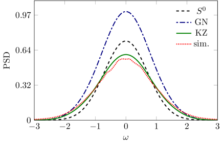
Figure 5: Comparing the (normalized) PSD of the GN and KZ models with the simulated (sim.) PSD.

VII-C Differences in Energy Transfer Mechanisms

Since the GN model assumes a Gaussian distribution, only $\Re(\mu_{lmnk})$ and $\Re(\mu_{lmnrpq})$ are responsible for spectrum evolution. In contrast, changes in the KZ PSD stem merely from $\Im(\mu_{lmnk})$. Because of the important factor $j$ in the NLS equation, $\Re(\mu_{lmnk})$ does not contribute to changes in PSD. Arbitrary non-Gaussian statistics can occur along $\Re(\mu_{lmnk})$ without impacting the PSD. Under the assumptions of the GN model (that the probability distribution is Gaussian in evolution), $\Im(\mu_{lmnk})=0$ and the KZ model (correctly) predicts a stationary spectrum. Consequently, deviations from Gaussianity are necessary for any spectral change.

A problem with the signal perturbation, and consequently with the GN model, is that here one works with moments, not the cumulants as in the KZ model. Moments of a scalar Gaussian random variable $X$, are $\mathsf{E}|X|^{2n}=(\mathsf{E}|X|^{2})^{n}(2n-1)!!$, where $n!!=n(n-2)(n-4)\cdots$, which grow with $n$. Higher-order moments cannot be ignored in the analysis. In contrast, higher-order cumulants are zero for Gaussian distribution and as the amplitude is increased, they are gradually generated sequentially in increasing order. The fact that cumulants are centered around a Gaussian distribution makes them suitable for use in a perturbation theory around the linear solution.

VII-D Differences in Probability Distributions

From the previous discussion, it follows that signal distribution in the KZ model is a zero-mean non-Gaussian distribution with the following moments: Asymmetric moments are zero; 2-point moment is given by the KZ PSD (49); 4-point moment is given by (47); other higher order moments are given in terms of the $2$- and $4$-point moments according to (73), with zero $2n$-point cumulants, $n\geq 3$.

VIII Application to WDM

One application of the PSD is to estimate the interference power in WDM systems. In models where the XPM amounts to a constant phase shift, the interference at frequency $k$ is non-degenerate FWM, as well as part of the degenerate FWM; see Fig. 1 and Example 1. However, in the WDM literature often the whole FWM is treated as interference. That is to say, all of the nonlinearity $\mathcal{N}_{k}$ in the NLS equation (20) is treated as noise. The corresponding spectra $S_{k}^{\text{KZ}}$ and $S_{k}^{\text{GN}}$ include self- and cross-channel interference.

Consider a WDM system with $2N+1$ users, each having bandwidth $\Omega_{s}$. In WDM the following (baseband) signal is sent over the channel

$$q(t,0)=\sum\limits_{m=-N}^{N}\left(\sum\limits_{l=1}^{M}a_{m}^{l}\phi^{l}(t)\right)e^{jm\Omega_{s}t},$$ (51)

where $l$ and $m$ are time and user indices, $\Omega_{s}$ is the user bandwidth, and $\phi^{l}(t)$ is an orthonormal basis for the space of finite-energy $T$-periodic signals with Fourier transform in $[-\Omega_{s}/2,\Omega_{s}/2]$. Finally, $a_{m}^{l}$ is a sequence of complex-valued random variables, independent between users, but potentially correlated within each user, i.e.,

$$\mathsf{E}a_{m}^{l}a_{m^{\prime}}^{l^{\prime}*}=\mu^{ll^{\prime}}_{mm}(a)\delta_{mm^{\prime}},$$

where $\mu^{ll^{\prime}}_{mm}(a)\stackrel{{\scriptstyle\Delta}}{{=}}\mathsf{E}a_{m}^{l}a_{m}^{l^{\prime}*}$ is the symbols correlation function of the user $m$, due to, e.g., channel coding. The set of frequencies of the user $m$, $-N\leq m\leq N$, is

$$A_{m}=\Bigl{\{}m\Omega_{s}+k\Omega_{0}\>|\>-N_{0}/2\leq k<N_{0}/2\Bigr{\}},$$

where $N_{0}\stackrel{{\scriptstyle\Delta}}{{=}}\lfloor\Omega_{s}/\Omega_{0}\rfloor$ and $\Omega_{0}\stackrel{{\scriptstyle\Delta}}{{=}}2\pi/T$.

VIII-A Stationary Gaussian WDM Signals

In this case, the assumptions of the GN and KZ models are satisfied. The interference “spectrum” is

$$S_{k}^{\text{NL}}=8\sum\limits_{lmn\>\in\>\textnormal{nr}_{k}}|H_{lmnk}|^{2}T_{lmnk},$$

where for the KZ model $T_{lmnk}$ is the collision term, and for the GN model $T_{lmnk}=S_{l}S_{m}S_{n}$. The intra (self)-channel interference for the central user $m=0$ is the part of the sum in $S_{k}^{\text{NL}}$ where $l,m,n\in A_{0}$. This is somewhat similar to SPM. The rest of terms, where at least one index is in the complement set $\bar{A}_{0}$, is the inter-channel interference. This is divided into three parts: 1) exactly two indices are in $A_{0}$ (1-wave interference) 2) exactly one index is in $A_{0}$ (2-wave interference) 3) no index is in $A_{0}$ (3-wave interference). The 1-wave interference has fewer terms than the others and can be ignored. The 2-wave interference is akin to XPM but is not similarly averaged out and should be accounted for.

Note that the net interference is zero in the KZ model, i.e., $S_{k}^{\text{NL}}$ is negative for some $k$.

VIII-B Non-stationary non-Gaussian WDM Signals

The correlation function of the WDM signal (51) is

$$R(t_{1},t_{2}) = \sum\limits_{mll^{\prime}}\mu_{mm}^{ll^{\prime}}(a)\phi^{l}(t_{1})\phi^{l^{\prime}*}(t_{2})\exp(-jm\Omega_{s}(t_{2}-t_{1}))$$

$$\overset{(a)}{=} {\mathcal{P}}_{0}\sum\limits_{l=1}^{M}\phi^{l}(t_{1})\phi^{l*}(t_{2})E(t_{2}-t_{1}),$$

where $E(x)\stackrel{{\scriptstyle\Delta}}{{=}}\sum_{m}\exp(-jm\Omega_{s}x)$ and step $(a)$ follows under the additional assumption that $a_{m}^{l}$ is i.i.d., so that $\mu_{mm}^{ll^{\prime}}={\mathcal{P}}_{0}\delta_{ll^{\prime}}$, ${\mathcal{P}}_{0}\stackrel{{\scriptstyle\Delta}}{{=}}\mathsf{E}|a_{m}^{l}|^{2}$. Unless in special cases, e.g., $\phi^{l}(t)=\exp(jl\Omega_{0}t)$, the input signal is not a stationary process. This can be seen in the frequency domain too. The Fourier series coefficients are

$$q_{k}=\sum\limits_{lm}a_{m}^{l}\phi_{mN_{0}+k}^{l},$$ (52)

where

$$\phi^{l}_{k}=\begin{cases}\mathcal{F}_{s}(\phi^{l}(t))(k),&-N_{0}/2\leq k<N_{0}/2,\\ 0,&\text{otherwise}.\end{cases}$$

The orthogonality of $\phi^{l}(t)e^{jn\Omega_{s}t}$ and $\phi^{l^{\prime}}(t)e^{jn^{\prime}\Omega_{s}t}$ in the frequency domain reads

$$\sum\limits_{k=-\frac{N_{0}}{2}}^{\frac{N_{0}}{2}-1}\phi_{k+nN_{0}}^{l}\phi_{k+n^{\prime}N_{0}}^{*l^{\prime}}=\delta_{ll^{\prime}}\delta_{nn^{\prime}}.$$

The 2-point spectral moment at $z=0$ is

$$\mu_{12} = {\mathcal{P}}_{0}\sum\limits_{lm}\phi_{mN_{0}+k_{1}}^{l}\phi_{mN_{0}+k_{2}}^{*l}.$$ (53)

In general $\mu_{12}\neq\mu_{11}\delta_{12}$, unless in special cases, e.g., if $k_{1}$ and $k_{2}$ belong to two different users, or $\phi^{l}_{k}=\phi_{0}\delta_{k}$, or $\phi^{l}_{k}=\phi_{0}\exp(j\frac{2\pi}{M}kl)$.

In addition to the stationarity Assumption b), Gaussianity Assumption c) may also not hold in WDM. In particular the input distribution is arbitrary. For non-Gaussian inputs, the cumulant $\kappa_{123456}(0)$ should be included.

The correlations and non-Gaussian input statistics can be introduced into the GN and KZ models using $\mu_{ij}$ and $\kappa_{123456}$. Repeating the analysis in the paper, the GN and KZ PSDs in WDM are

$$S_{k}^{\text{GN}} = S^{0}_{k}+4\sum\limits_{\textnormal{nr}_{k},\textnormal{nr}_{k^{\prime}}}H_{lmnk}H_{l^{\prime}m^{\prime}n^{\prime}k}\mu_{lmn^{\prime}l^{\prime}m^{\prime}n},$$

$$S_{k}^{\text{KZ}} = S^{0}_{k}+8\sum\limits_{\textnormal{nr}_{k}}|H_{lmnk}|^{2}T_{lmnk},$$

where

$$T_{lmnk} \stackrel{{\scriptstyle\Delta}}{{=}} \frac{1}{2}\sum\limits_{l^{\prime}m^{\prime}n^{\prime}}\Bigl{(}\mu_{l^{\prime}mm^{\prime}nn^{\prime}k}\delta_{l^{\prime}m^{\prime}n^{\prime}k}+\mu_{ll^{\prime}m^{\prime}nn^{\prime}k}\delta_{l^{\prime}m^{\prime}n^{\prime}m}$$ (54)

$$-\>\mu_{lmn^{\prime}l^{\prime}m^{\prime}k}\delta_{l^{\prime}m^{\prime}n^{\prime}n}-\mu_{lmn^{\prime}l^{\prime}m^{\prime}n}\delta_{l^{\prime}m^{\prime}n^{\prime}k}\Bigr{)}.$$

The 6-point moment is

$$\mu_{123456} = \sum\limits_{l_{1-6}m_{1-6}}\mu_{123456}^{123456}(a)\phi_{m_{1}N_{0}+k_{1}}^{l_{1}}\phi_{m_{2}N_{0}+k_{2}}^{l_{2}}\phi_{m_{3}N_{0}+k_{3}}^{l_{3}}$$ (55)

$$\qquad\qquad\times\>\phi_{m_{4}N_{0}+k_{4}}^{*l_{4}}\phi_{m_{5}N_{0}+k_{5}}^{*l_{5}}\phi_{m_{6}N_{0}+k_{6}}^{*l_{6}}$$

$$= \mu_{14}\mu_{25}\mu_{36}+\mu_{14}\mu_{26}\mu_{35}+\mu_{15}\mu_{24}\mu_{36}$$

$$+\>\mu_{15}\mu_{26}\mu_{34}+\mu_{16}\mu_{24}\mu_{35}+\mu_{16}\mu_{25}\mu_{34}$$

$$+\>\kappa_{123456},$$

where $\mu_{ij}$ is given in (53), and we used

$$\mu_{123456}^{123456}(a) \stackrel{{\scriptstyle\Delta}}{{=}} \mathsf{E}a_{m_{1}}^{l_{1}}a_{m_{2}}^{l_{2}}a_{m_{3}}^{l_{3}}a_{m_{4}}^{*l_{4}}a_{m_{5}}^{*l_{5}}a_{m_{6}}^{*l_{6}}$$

$$= {\mathcal{P}}^{3}\Bigl{(}\delta_{14}^{14}\delta_{25}^{25}\delta_{36}^{36}+\delta_{14}^{14}\delta_{26}^{26}\delta_{35}^{35}+\delta_{15}^{15}\delta_{24}^{24}\delta_{36}^{36}$$

$$+\>\delta_{15}^{15}\delta_{26}^{26}\delta_{34}^{34}+\delta_{16}^{16}\delta_{24}^{24}\delta_{35}^{35}+\delta_{16}^{16}\delta_{25}^{25}\delta_{34}^{34}\Bigr{)}$$

$$+\>\kappa_{123456}^{123456}(a),$$

where $\delta_{m_{1}m_{2}}^{l_{1}l_{2}}\stackrel{{\scriptstyle\Delta}}{{=}}\delta_{m_{1}m_{2}}\delta_{l_{1}l_{2}}$.

For i.i.d. symbols, from (76) and (77), we have $\kappa_{12}^{12}(a)=\tilde{S}_{12}(a)\delta_{12}^{12}$, $\kappa_{1234}^{1234}(a)=\tilde{S}_{1234}(a)\delta_{12}^{12}\delta_{23}^{23}\delta_{34}^{34}$, $\kappa_{123456}^{123456}(a)=\tilde{S}_{123456}(a)\delta_{12}^{12}\delta_{23}^{23}\delta_{34}^{34}\delta_{45}^{45}\delta_{56}^{56}$, and so on, with cumulant densities

$$\tilde{S}_{12}(a) = \mathsf{E}|a|^{2},$$

$$\tilde{S}_{1234}(a) = \mathsf{E}|a|^{4}-2\mathsf{E}^{2}|a|^{2},$$ (56)

$$\tilde{S}_{123456}(a) = \mathsf{E}|a|^{6}-9\mathsf{E}|a|^{2}\mathsf{E}|a|^{4}+12\mathsf{E}^{3}|a|^{2}.$$ (57)

The simplifications of Section VI-A in the case of uncorrelated Gaussian signals, due to integration over delta functions, do not occur anymore. If $\phi^{l}(t)=p(t-lT/M)$, where $p(t)$ is a pulse shape in time interval $[0,T/M]$, then $\phi_{k}^{l}=p_{k}\exp(j2\pi kl/M)$ and

$$\mu_{12} = {\mathcal{P}}(2N+1)p_{1}p_{2}^{*}\sum\limits_{l=1}^{M}\exp(j2\pi l(k_{1}-k_{2})/M)$$

$$= {\mathcal{P}}(2N+1)Mp_{1}p_{2}^{*}\delta_{12}.$$

In this case there is no correlation and PSDs are modified only via $\kappa_{123456}$.

Remark 3.

The accuracy of the GN model has been improved in the enhanced GN model (EGN) [11, 12, 13, 14]. In the EGN model, correction terms are introduced to the GN model to account for non-Gaussianity. The forth-order correction term in [11] is identified with the cumulant (56) in the KZ model. Likewise, the correction terms $\Phi_{a}$ and $\Psi_{a}$ in [14, Eq. 6] are, respectively, identified with cumulants (56) and (57). Furthermore, KZ model illustrates how infinitely many such terms can be added methodically.

VIII-C Phase Interference

The power spectral density of the nonlinear term in the NLS equation does not suggest that one should consider nonlinearity as additive noise. In fact, the PSD obviously does not capture cross-phase interference. In the energy-preserving NLS equation, XPM is a constant phase shift, as shown, e.g., in (20). However, in WDM, from (52), the signal energy is

$$\sum\limits_{k=1}^{(2N+1)N_{0}}|q_{k}|^{2}=\sum\limits_{lm}|a_{m}^{l}|^{2}\phi_{mN_{0}+k}^{l}\phi_{mN_{0}+k}^{*l}.$$ (58)

Typically, the per-user power is a known constant, however, in an optical mesh network, the power of interfering users may not be known. Energy is also not preserved in the presence of loss. In such cases where XPM is no longer a constant phase shift, part of the sum (58) where $m\neq 0$ acts as cross-phase interference for the center user.

The interference resulting from XPM is discussed in [15]. This is done by substituting the WDM input signal (51) into the approximate solution (23), sorting out interference terms, and naming XPM and FWM.

IX KZ and GN PSDs in Multi-Span Systems

The PSDs (27) and (49) hold for one span of lossless fiber with second-order dispersion. In this section, we include loss and higher order dispersion, and generalize (27) and (49) to multi-span links with amplification.

We consider a multi-span optical system with $N$ spans, each of length $\epsilon$, in a fiber of total length $z$, $z=N\epsilon$. Pulse propagation in the overall link is governed by

$$\partial_{z}q_{\omega}(z) = j\left(\frac{j\alpha(z)}{2}-\beta(\omega)\right)q_{\omega}(z)-j\gamma\mathcal{N}_{\omega}(q,q,q)(z)$$ (59)

$$+\>\left(\sum\limits_{n=1}^{N}\frac{G_{n}(z)}{2}\delta(z-n\epsilon)\right)q_{\omega}(z),$$

where $\alpha(z)$ is (power) loss exponent, $G_{n}(z)\stackrel{{\scriptstyle\Delta}}{{=}}\int_{(n-1)\epsilon}^{n\epsilon}\alpha(l)\mathrm{d}l$ is the lumped gain exponent at the end of span $n$, $\gamma$ is the nonlinearity coefficient and

$$\beta(\omega)=\beta_{0}+\beta_{1}(\omega-\omega_{0})+\frac{\beta_{2}}{2}(\omega-\omega_{0})^{2}+\cdots,$$

is the dispersion function (also known as the wavenumber or propagation constant).

Lumped power amplification at the end of each span restores the linear part of PSD, however, since loss is distributed, it does not normalize the nonlinear part. As a result, signal amplification leads to a growth of FWM interference, which we calculate in this section.

Remark 4.

Loss and periodic amplification have been discussed in [16] in the context of fiber lasers. Here a modified kinetic equation approach is taken to describe laser spectrum. Changes in spectrum (kinetics) in [16] occur due to loss and periodic amplification, i.e., perturbations to integrability. In the transmission problem, on the other hand, there is kinetics even with no loss and amplification in integrable model; see (49), as well as numerical simulations of the actual PSD in the literature of the GN model, and [8]. In our problem the hypothesis of delta concentration $\delta(\Omega_{123\omega})$ of the standard turbulence [3] does not hold with desired accuracy. For parameters where the models of [16] and this paper coincide, the observations are in agreement. In this section, we generalize (49).

IX-1 GN Model

Consider the NLS equation (59) with loss, dispersion $\beta(\omega)$, and amplification. Let

$$F(z)\stackrel{{\scriptstyle\Delta}}{{=}}\int_{0}^{z}\left(\alpha(l)-\sum\limits_{n=1}^{N}G_{n}(l)\delta(l-n\epsilon)\right)\mathrm{d}l.$$

Comparing (59) with the dimensionless NLS equation, we identify $\omega^{2}z\rightarrow jF(z)/2-\beta(\omega)z$. Therefore

$$\Omega_{123\omega}z=\left(\omega_{1}^{2}+\omega_{2}^{2}-\omega_{3}^{*2}-\omega^{2}\right)z$$

in signal (23) and PSD (49) is replaced with

$$\bar{\Omega}_{123\omega}z=jF(z)-\Omega_{123\omega}z,$$

where now

$$\Omega_{123\omega}\stackrel{{\scriptstyle\Delta}}{{=}}\beta(\omega_{1})+\beta(\omega_{2})-\beta(\omega_{3})-\beta(\omega).$$

The GN PSD (27) is modified to

$$S_{\omega}(z)=e^{-F(z)}\left(S_{\omega}(0)+2\gamma^{2}\int|\tilde{H}_{123\omega}|^{2}S_{1}S_{2}S_{3}\delta_{123\omega}\mathrm{d}\omega_{123}\right),$$

where

$$\tilde{H}_{123\omega} \stackrel{{\scriptstyle\Delta}}{{=}} -j\int\limits_{0}^{z}e^{j\bar{\Omega}_{123\omega}l}\mathrm{d}l$$ (60)

$$= -j\int\limits_{0}^{z}e^{-(F(l)+j\Omega_{123\omega}l)}\mathrm{d}l.$$

Several cases can be derived from (60).

Single-span lossy fiber

In a single-span fiber with constant loss $\alpha$ and no amplification, $G=0$ and $F(z)=\alpha z$. Thus $\tilde{H}_{123\omega}=H_{123\omega}(j\alpha-\Omega_{123\omega})(z)$. This shows the effect of loss and higher order dispersion.

Multi-span links

In a multi-span link with constant loss $\alpha$,

$$F(l)=\alpha l-\alpha\epsilon\sum_{i=1}^{N}U(l-i\epsilon)=\alpha(l-n\epsilon),\>n=\lfloor l/\epsilon\rfloor,$$ (61)

where $U(x)$ is the Heaviside step function. Thus

$$\tilde{H}_{123\omega} = -j\int\limits_{0}^{z}e^{\left(-\alpha l+\alpha\epsilon\sum\limits_{n=1}^{N}U(l-n\epsilon)-j\Omega_{123\omega}l\right)}\mathrm{d}l$$ (62)

$$= -j\sum\limits_{n=0}^{N-1}\int\limits_{n\epsilon^{-}}^{(n+1)\epsilon^{-}}e^{\left(-\alpha(l-n\epsilon)-j\Omega_{123\omega}l\right)}\mathrm{d}l$$

$$= -j\sum\limits_{n=0}^{N-1}e^{-jn\epsilon\Omega_{123\omega}}\int\limits_{0}^{\epsilon}e^{j\left(j\alpha-\Omega_{123\omega}\right)z^{\prime}}\mathrm{d}z^{\prime}$$

$$= H(j\alpha-\Omega_{123\omega})(\epsilon)G_{123\omega}^{\text{GN}},$$

where

$$G_{123\omega} \stackrel{{\scriptstyle\Delta}}{{=}} \sum\limits_{n=0}^{N-1}e^{-jn\epsilon\Omega_{123\omega}}=\frac{1-e^{-jz\Omega_{123\omega}}}{1-e^{-j\epsilon\Omega_{123\omega}}}$$ (63)

$$= e^{-j\frac{\Omega}{2}(z-\epsilon)}\frac{\sin(z\Omega_{123\omega}/2)}{\sin(\epsilon\Omega_{123\omega}/2)}.$$

Therefore, the GN PSD of multi-span link is given by the same equation (27), with $H(\Omega_{123\omega})(z)$ replaced with $(\gamma/2)H(j\alpha-\Omega_{123\omega})(\epsilon)G_{123\omega}$. Note that $\tilde{H}$ describes the FWM growth in both the signal and PSD. For further clarification, see Appendix B.

IX-2 KZ Model

Considering the analysis of Section VI-A, factors $-(\mathrm{d}F(z)/\mathrm{d}z)S_{k}$ and $-2(\mathrm{d}F(z)/\mathrm{d}z)S_{lmnk}$ appear, respectively, in the right hand sides of moment equations (44) and (46). The KZ PSD is

$$S_{k}(z) = e^{-F(z)}\Bigl{(}S_{k}^{0}+\>2\gamma\sum\limits_{\textnormal{nr}_{k}}\int\limits_{0}^{z}e^{F(z^{\prime})}\Im(S_{lmnk}(z^{\prime}))\mathrm{d}z^{\prime}\Bigr{)},$$ (64)

where

$$\Im(S_{lmnk}(z)) = 2\gamma\int\limits_{0}^{z}e^{-2(F(z)-F(z^{\prime}))}\cos\left(\Omega_{lmnk}(z-z^{\prime})\right)$$ (65)

$$\qquad\times\>T_{lmnk}(z^{\prime})\mathrm{d}z^{\prime}.$$

Here, as in (47) and (48), we assumed that $S_{lmnk}(0)$ is real-valued for quasi-Gaussian input.

We substitute (65) into (64) and solve the resulting fixed-point equation iteratively starting from $S_{k}(z)=0$. The first iterate gives $S_{k}^{(0)}(z)=\exp(-F(z))S_{k}^{0}$. In the next iterate, the collision term is found to be $T_{lmnk}(z)=\exp(-3F(z))T_{lmnk}(0)$, which is no longer constant. Using this collision term in (65), and subsequently in (64), we obtain

$$S_{k}^{\text{KZ}}=e^{-F(z)}\left(S_{k}^{0}+2\gamma^{2}\sum\limits_{lmn\>\in\>\textnormal{nr}_{k}}|\tilde{H}_{lmnk}|^{2}T_{lmnk}\right),$$ (66)

where

$$|\tilde{H}_{lmnk}|^{2} = 2\int\limits_{0}^{z}\int\limits_{0}^{z^{\prime}}e^{-(F(z^{\prime})+F(l))}\cos\left(\Omega(z^{\prime}-l)\right)\mathrm{d}l\mathrm{d}z^{\prime}.$$ (67)

The integration in (67) is over a triangle. However the function under integration is symmetric in $l$ and $z^{\prime}$, i.e., around the line $l=z^{\prime}$. Thus integration can be extended to the rectangle:

$$|\tilde{H}_{lmnk}|^{2} = \int\limits_{0}^{z}\int\limits_{0}^{z}e^{-(F(z^{\prime})+F(l))}\cos\left(\Omega(z^{\prime}-l)\right)\mathrm{d}l\mathrm{d}z^{\prime}$$ (68)

$$= \left|\int\limits_{0}^{z}e^{-(F(l)+j\Omega_{lmnk}l)}\mathrm{d}l\right|^{2}.$$

This is the same as $|\tilde{H}_{123\omega}|^{2}$ in (60) for the GN model, with $123\omega\rightarrow lmnk$.

It follows that in all cases, the PSD kernels $|H_{123\omega}|^{2}$ and $|\tilde{H}_{123\omega}|^{2}$ in the GN and KZ models are the same.

Single-span lossy fiber

For constant $\alpha$, the PSD is given by (66) with $F(z)=\alpha z$ and

$$|\tilde{H}_{lmnk}|^{2} = |H(j\alpha-\Omega_{lmnk})(z)|^{2}$$

$$= 2e^{-\alpha z}\Bigl{(}\frac{\cosh(\alpha z)-\cos(\Omega z)}{\alpha^{2}+\Omega^{2}}\Bigr{)}.$$

This shows that in the presence of loss and physical parameters, just as in the GN model, the KZ PSD, after amplification $\exp(\alpha z)$ at the end of the link, is the same as (49), with $H(\Omega_{lmnk})(z)$ replaced with $(\gamma/2)H(j\alpha-\Omega_{lmnk})(z)$.

Multi-span links

In the multi-span link, at the end of the link $F(z)=0$. The PSD is given by (66) with $F(z)=0$ and

$$\tilde{H}_{123\omega}=H(j\alpha-\omega_{123\omega})(\epsilon)G_{123\omega}.$$

with the same $G_{123\omega}$ given by (63).

X Conclusions

A mathematical framework based on the WWT theory is presented to study the evolution of multi-point cumulants in nonlinear dispersive partial differential equations with random input data. This framework is used to explain how energy is distributed among Fourier modes in the nonlinear Schrödinger equation, by considering interactions among four Fourier modes and studying the role of the resonant, non-resonant, and trivial quartets in the dynamics. As an application, a PSD, termed KZ model, is proposed for calculating the interference power in WDM systems.

The GN model, often used in optical communication, suggests a spectrum evolution, in agreement with numerical and experimental fiber-optic transmissions. That seemingly conflicts with the WWT which predicts a stationary spectrum for integrable models. It is shown that if the kinetic equation of WWT is solved to the next order in nonlinearity, a PSD is obtained which is similar to the GN PSD. The two models are explained mathematically and connected with each other. The analysis shows that the kinetic equation of the NLS equation better describes the PSD. This is not surprising, because the GN model applies perturbation theory to the signal equation, while the WWT applies it directly to the PSD differential equation. The assumptions of the WWT are verified in data communications and the basic KZ PSD is extended to various cases encountered in communications. The GN model is also simplified for clarity and comparison.

Appendix A Moments and Cumulants

A-A A Property of the Stationary Processes

We make use of the following simple lemma throughout the paper, which says that the spectral moments of a stationary process are supported on the stationary manifold (7).

Lemma 2.

If $q(t)$ is a strongly stationary stochastic process with finite power and existing Fourier transform, then $\mu_{1\cdots 2n}=S_{1\cdots 2n}\delta_{1\cdots 2n}$.

Proof.

Define

$$E(t_{1},\cdots,t_{2n})\stackrel{{\scriptstyle\Delta}}{{=}}\exp\bigl{(}j(s_{1}\omega_{1}t_{1}+\cdots+s_{2n}\omega_{2n}t_{2n})\bigr{)}.$$

Shifting $t_{i}$ by $t_{1}$, it can be verified that

$$E(t_{1},\cdots,t_{2n})=\exp(j\Delta\omega t_{1})E(0,t_{2}-t_{1},\cdots,t_{2n}-t_{1}),$$

(69)

where $\Delta\omega\stackrel{{\scriptstyle\Delta}}{{=}}\sum_{i=1}^{2n}s_{i}\omega_{i}$. Expressing $q_{i}$ in (6) using the inverse Fourier transform, the (strong) stationarity property implies that

$$\mu_{1\cdots 2n} = \mathsf{E}\Bigl{(}q_{1}\cdots q^{*}_{2n}\Bigr{)}$$

$$= \int R(t_{1},\cdots,t_{2n})E(t_{1},\cdots,t_{2n})\mathrm{d}t_{1-2n}$$

$$= \int R(0,t_{2}-t_{1},\cdots,t_{2n}-t_{1})$$

$$\times E(0,t_{2}-t_{1},\cdots,t_{2n}-t_{1})\exp(j\Delta\omega t_{1})\mathrm{d}t_{1-2n}$$

$$= \delta(\Delta\omega)\int R(0,\tau_{2},\cdots,\tau_{2n})E(0,\tau_{2},\cdots,\tau_{2n})\mathrm{d}\tau_{2-2n}$$

$$= S_{1\cdots 2n}\delta(\Delta\omega),$$

where $\tau_{i}\stackrel{{\scriptstyle\Delta}}{{=}}t_{i}-t_{1}$ and

$$S_{1\cdots 2n}\stackrel{{\scriptstyle\Delta}}{{=}}\mathcal{F}(R(0,\tau_{2},\cdots,\tau_{2n}))(0,s_{2}\omega_{2},\cdots,s_{2n}\omega_{2n}).$$

∎

The lemma essentially follows from the shift property of the exponential function (69). A more general statement is the Wiener-Khinchin theorem.

As a corollary, if $q(t)$ is stationary, $\mu_{\omega\omega}$ is infinity.

A-B Cumulants

Let $q=(q_{1},\cdots,q_{n})$ be a complex-valued random vector. We define the joint moment generating function of $q$, $\Phi:\mathbb{C}^{n}\mapsto\mathbb{R}$, as

$$\Phi(\zeta) \stackrel{{\scriptstyle\Delta}}{{=}} \mathsf{E}\exp\left(\Re(\zeta^{H}q)\right)$$ (70)

$$= \sum\limits_{r,s=0}^{\infty}\frac{1}{r!s!}\mu^{r}_{s}\zeta^{r}\zeta^{*s},$$ (71)

where $r,s$ are $n$-dimensional multi-indices, $r!=\prod_{k=1}^{n}r_{k}!$, $r_{k}=0,1,\cdots$, $\zeta^{r}=\prod_{k=1}^{n}\zeta_{k}^{r_{k}}$, and

$$\mu^{r}_{s}=\mathsf{E}q^{*r}q^{s},$$

is the $|r+s|$-point moment. It can be verified that

$$\mu^{r}_{s}=\frac{\partial^{r+s}}{\partial\zeta^{r}\zeta^{*s}}\Phi(\zeta)\Bigr{|}_{\zeta=0}.$$ (72)

The joint cumulant generating function is $\Psi(\tau)=\log\Phi(\tau)$. The cumulants $\kappa_{s}^{r}$ are defined from multi-variate Taylor expansion similar to (71) and (72).

Note that with the notation of Section II, $\mu_{1\cdots 2n}=\mu_{r}^{s}$ with $|r|=|s|=n$. Cumulants $\kappa$ relate to cumulant densities $\tilde{S}$ via

$$\kappa_{1\cdots 2n}=\tilde{S}_{1\cdots 2n}\delta_{1\cdots 2n}.$$

Joint moments can be obtained from joint cumulants by applying chain rule of differentiation to $\Phi=\exp\Psi$, obtaining

$$\mu_{1\cdots 2n}=\sum\limits_{p\in P}\prod\limits_{a\in p}\kappa_{a},$$ (73)

where $P$ is the set of all partitions of $(1,2,\cdots,2n)$. The expression is considerably simplified for a zero-mean process, which is assumed throughout this paper. Further simplifications occur by noting that the asymmetric moments and cumulants are zero. With these simplifications, the first four relations are:

$$\mu_{1} = \kappa_{1}=0,$$

$$\mu_{12} = \kappa_{12},$$

$$\mu_{1234} = \kappa_{13}\kappa_{24}+\kappa_{14}\kappa_{23}+\kappa_{1234},$$

$$\mu_{123456} = \Bigl{(}\kappa_{14}\kappa_{25}\kappa_{36}+\kappa_{14}\kappa_{26}\kappa_{35}+\kappa_{15}\kappa_{24}\kappa_{36}$$ (74)

$$+\>\kappa_{15}\kappa_{26}\kappa_{34}+\kappa_{16}\kappa_{24}\kappa_{35}+\kappa_{16}\kappa_{24}\kappa_{35}\Bigr{)}$$

$$+\>\Bigl{(}\kappa_{14}\kappa_{2356}+\kappa_{15}\kappa_{2346}+\kappa_{16}\kappa_{2345}$$

$$+\>\kappa_{24}\kappa_{1234}+\kappa_{25}\kappa_{1356}+\kappa_{26}\kappa_{1345}$$

$$+\>\kappa_{34}\kappa_{1256}+\kappa_{35}\kappa_{1246}+\kappa_{36}\kappa_{1245}\Bigr{)}$$

$$+\>\kappa_{123456}.$$

For a stationary process $\kappa_{ij}=\mu_{ij}=S_{ii}\delta_{ij}$ and we obtain (8). Since higher-order cumulants are smaller than the second-order cumulant for quasi-Gaussian distributions, we can assume $\kappa_{lmnk}=\kappa_{lmnl^{\prime}m^{\prime}n^{\prime}}=0$, thereby obtaining (9).

Cumulants can be obtained from moments by applying Möbius inversion formula to (73), obtaining

$$\kappa_{1\cdots 2n}=\sum\limits_{p\in P}\prod_{a\in p}(-1)^{|p|-1}(|p|-1)!\mu_{a},$$ (75)

where $|p|$ is the number of the sets in the partition $p$, i.e., the number of products in $\mu_{a}$. Setting asymmetric moments to zero, we have

$$\kappa_{12} = \mu_{12}$$

$$\kappa_{1234} = -\mu_{13}\mu_{24}-\mu_{14}\mu_{23}+\mu_{1234}$$ (76)

$$\kappa_{123456} = 2\Bigl{(}\mu_{14}\mu_{25}\mu_{36}+\mu_{14}\mu_{26}\mu_{35}+\mu_{15}\mu_{24}\mu_{36}$$ (77)

$$+\>\mu_{15}\mu_{26}\mu_{34}+\mu_{16}\mu_{24}\mu_{35}+\mu_{16}\mu_{25}\mu_{34}\Bigr{)}$$

$$-\>\bigl{(}\mu_{14}\mu_{2356}+\mu_{15}\mu_{2346}+\mu_{16}\mu_{2345}$$

$$+\>\mu_{24}\mu_{1234}+\mu_{25}\mu_{1356}+\mu_{26}\mu_{1345}$$

$$+\>\mu_{34}\mu_{1256}+\mu_{35}\mu_{1246}+\mu_{36}\mu_{1245}\Bigr{)}$$

$$+\>\mu_{123456}.$$

For i.i.d. zero-mean random variables, any variables matching in $\mu_{1\cdots 2n}$ is canceled by terms prior to $\mu_{1\cdots 2n}$ in (77) and (76), except when all variables are equal. Thus $\kappa_{1234}=\left(\mathsf{E}|q_{k}|^{4}-2\mathsf{E}^{2}|q_{k}|^{2}\right)\delta_{12}\delta_{23}\delta_{34}$ and so on.

Appendix B GN PSD in Multi-span Links

In Section IX, the multi-span PSDs were obtained in a unified manner by introducing function $F(z)$ and modifying kernels $H_{123\omega}$. One consequence is that multi-span PSDs can (expectedly) be obtained from single-span PSDs, regardless of whether the interference is added coherently or not in the signal picture. The multi-span GN PSD (62) is known in the literature [2]. It is presumably obtained in the manner described below; however, it is often intuitively explained rather than fully derived.

At the end of the first span, after amplification, we have

$$q_{\omega}(\epsilon) = e^{-j\epsilon\beta(\omega)}\Bigl{\{}q_{\omega}(0)-j\gamma N_{\omega}(q,q,q|H)(0,\epsilon)\Bigr{\}},$$

where

$$N_{\omega}(q,q,q|H)(z,z^{\prime}) \stackrel{{\scriptstyle\Delta}}{{=}} \int H_{123\omega}(j\alpha-\Omega_{123\omega})(z^{\prime}-z)$$

$$\times\>q_{1}(z)q_{2}(z)q_{3}^{*}(z)\mathrm{d}\omega_{123}.$$

At the end of the second span

$$q_{\omega}(2\epsilon) = e^{-j\epsilon\beta(\omega)}\Bigl{\{}q_{\omega}(\epsilon)-j\gamma N_{\omega}(q,q,q|H)(\epsilon,2\epsilon)\Bigr{\}}$$

$$= e^{-j2\epsilon\beta(\omega)}q_{\omega}(0)-j\gamma e^{-j2\epsilon\beta(\omega)}N_{\omega}(q,q,q|H)(0,\epsilon)$$

$$-j\gamma e^{-j\epsilon\beta(\omega)}N_{\omega}(q,q,q|H)(\epsilon,2\epsilon).$$

The last term contains $q_{\omega}(\epsilon)$, which itself is the sum of a linear and a nonlinear term. In agreement with the first-order approach of the GN model, all FWM terms are evaluated at the linear solution; the contribution of the nonlinear term to $q_{\omega}(2\epsilon)$ is of second order $\gamma^{2}$. We thus evaluate the last term at $\exp(-j\epsilon\beta(\omega))q_{\omega}(0)$:

$$\mathcal{N}_{\omega}(q,q,q|H)(\epsilon,2\epsilon)=\int H_{123\omega}(\epsilon)q_{1}(\epsilon)q_{2}(\epsilon)q_{3}^{*}(\epsilon)\delta_{123\omega}\mathrm{d}\omega_{123}$$

$$= e^{-j\epsilon\beta(\omega)}\int e^{-j\Omega\epsilon}H_{123\omega}(\epsilon)q_{1}(0)q_{2}(0)q_{3}^{*}(0)\delta_{123\omega}\mathrm{d}\omega_{123}$$

$$= e^{-j\epsilon\beta(\omega)}N_{\omega}(q,q,q|e^{-j\Omega\epsilon}H)(0,\epsilon).$$

Thus

$$q_{\omega}(2\epsilon) = e^{-2j\epsilon\beta(\omega)}\Bigl{\{}q_{\omega}(\epsilon)-j\gamma N_{\omega}\left(q,q,q|G_{1}H\right)(0,\epsilon)\Bigr{\}},$$

where $G_{1}\stackrel{{\scriptstyle\Delta}}{{=}}1+e^{-j\Omega\epsilon}$. By induction, we have

$$q_{\omega}(z) = e^{-jz\beta(\omega)}\Bigl{\{}q_{\omega}(0)-j\gamma N_{\omega}\left(q,q,q|GH\right)(0,\epsilon)\Bigr{\}},$$ (78)

where $G$ is given by (63). Squaring and averaging (78), we obtain the multi-span GN PSD.

References

• [1] K. Inoue, “Phase-mismatching characteristic of four-wave mixing in fiber lines with multistage optical amplifiers,” Opt. Lett., vol. 17, no. 11, pp. 801–803, Jun. 1992.
• [2] P. Poggiolini, “The GN model of non-linear propagation in uncompensated coherent optical systems,” IEEE J. Lightw. Technol., vol. 30, no. 24, pp. 3857–3879, Dec. 2012.
• [3] V. E. Zakharov, V. S. L’vov, and G. Falkovich, Kolmogorov Spectra of Turbulence I, ser. Nonlinear Dynamics.   Berlin, Germany: Springer-Verlag, 1992.
• [4] V. E. Zakharov, “Turbulence in integrable systems,” Stud. Appl. Math., vol. 122, no. 3, pp. 219–234, Apr. 2009.
• [5] V. E. Zakharov, F. Dias, and A. Pushkarev, “One-dimensional wave turbulence,” Phys. Rep., vol. 398, no. 1, pp. 1–65, Aug. 2004.
• [6] S. K. Turitsyn et al., “Optical wave turbulence,” in Advances in Wave Turbulence, ser. World Scientific.   Singapore: World Scientific, 2013, vol. 83, ch. 4.
• [7] A. Picozzi et al., “Optical wave turbulence: Toward a unified nonequilibrium thermodynamic formulation of statistical nonlinear optics,” Phys. Rep., vol. 542, no. 1, pp. 1–132, Mar. 2014.
• [8] P. Suret, A. Picozzi, and S. Randoux, “Wave turbulence in integrable systems: nonlinear propagation of incoherent optical waves in single-mode fibers,” Opt. Exp., vol. 19, no. 18, pp. 17 852–17 863, Aug. 2011.
• [9] M. I. Yousefi and F. R. Kschischang, “Information transmission using the nonlinear Fourier transform, Part I: Mathematical tools,” IEEE Trans. Inf. Theory, vol. 60, no. 7, pp. 4312–4328, Jul. 2014. [Online]. Available: http://arxiv.org/abs/1202.3653
• [10] M. I. Yousefi and X. Yangzhang, “Linear and nonlinear frequency-division multiplexing,” arXiv:1603.04389, Mar. 2015. [Online]. Available: http://arxiv.org/abs/1603.04389
• [11] R. Dar, M. Feder, A. Mecozzi, and M. Shtaif, “Properties of nonlinear noise in long, dispersion-uncompensated fiber links,” Opt. Exp., vol. 21, no. 22, pp. 25 685–25 699, Nov. 2013.
• [12] P. Serena and A. Bononi, “A time-domain extended Gaussian noise model,” IEEE J. Lightw. Technol., vol. 33, no. 7, pp. 1459–1472, Apr. 2015.
• [13] P. Poggiolini, G. Bosco, A. Carena, V. Curri, Y. Jiang, and F. Forghieri, “A simple and effective closed-form GN model correction formula accounting for signal non-Gaussian distribution,” IEEE J. Lightw. Technol., vol. 33, no. 2, pp. 459–473, Jan. 2015.
• [14] A. Carena, G. Bosco, V. Curri, Y. Jiang, P. Poggiolini, and F. Forghieri, “EGN model of non-linear fiber propagation,” Opt. Exp., vol. 22, no. 13, pp. 16 335–16 362, Jun. 2014.
• [15] A. Mecozzi and R.-J. Essiambre, “Nonlinear Shannon limit in pseudolinear coherent systems,” IEEE J. Lightw. Technol., vol. 30, no. 12, pp. 2011–2024, Jun. 2012.
• [16] D. V. Churkin et al., “Wave kinetics of random fibre lasers,” Nature Commun., vol. 2, no. 6214, pp. 1–6, Feb. 2015.