Spin-charge ordering induced by magnetic field in superconducting state: analytical solution in the two-dimensional self-consistent model

Abstract

Solutions of the Bogoliubov-de Gennes equations for the two-dimensional self-consistent Hubbard t-U-V model of superconductors with $d_{x^{2}-y^{2}}$ symmetry of the order parameter in the presence of a magnetic field are found. It is shown that spatial inhomogeneity of superconducting order parameter results in the emergence of stripe-like domains that are stabilized by applied magnetic field leading to emergence of space-modulated composite spin-charge-superconducting order parameter.

I Introduction

The accumulating experimental evidence suggests that the pseudogap phase could be a key issue in understanding the underlying mechanism of high-transition-temperature superconducting (high-T_c) copper oxides taill . Magnetotransport data in electron-doped copper oxide La_2-xCe_xCuO₄ suggests that linear temperature-dependent resistivity correlates with the electron pairing and spin-fluctuating scattering of the electrons greene . Simultaneously, in the hole-doped copper oxide YBa₂Cu₃O_y a large in-plane anisotropy of the Nernst effect sets in at the boundary of the pseudogap phase and indicates that this phase breaks four-fold rotational symmetry in the a-b plane, pointing to stripe or nematic order taill1 . Antiferromagnetic spin ordering in single crystals of underdoped ($x=0.10$) La_2-xSr_xCuO₄ induced by an applied magnetic was observed in magnetic neutron diffraction experiments aeppli2 . The authors found that applied magnetic field, that imposed the Abrikosov’s vortex lattice, also induced ‘striped’ antiferromagnetic order with the ordered moment $0.4\mu_{B}$ per Cu$2^{+}$, as suggested by muon spin relaxation data muon . The field-induced signal increased according to classical mean-field theory, suggesting an intrinsic mechanism aeppli2 . Besides, The field-induced signal proved to be resolution-limited, and the magnetic in-plane correlation length ($\zeta>400A$ ), was much greater than the superconducting coherence length ($\xi<20A$ ) and the inter-vortex spacing $a_{v}=130A$ for H$=14.5$T. The authors concluded that since superconducting coherence length $\xi$ defines the size of the vortices, coherent magnetism scaled with $\zeta$ must extend beyond the vortex core across the superconducting regions of the material, and hence, superconductivity and antiferromagnetism coexist throughout the bulk of the material aeppli2 . Motivated by these experimental results, we study here theoretically an analytically solvable model that manifests a coexistence of the stripe order and d-wave superconductivity. We found an exact solution of the Bogoliubov-de Gennes equations in the simple microscopic Hubbard t-U-V model indicating that the Abrikosov’s vortex core naturally gives rise to a stripe-ordered domain, i.e. coupled antiferromagnetic (AFM) electronic spin- and charge-density modulations. We show that the size of the stripe domain may exceed superconducting vortex’s core size $\xi_{s}$ and the inter-vortex distance in the Abrikosov’s lattice in the limit of weak magnetic fields $H\leq H_{c1}$. As far as we know, this is the first analytic solution of such type. Previously, coexistence of the stripe-order and Abrikosov’s vortices in the limit of high magnetic fields $H\sim H_{c2}$ has been investigated numerically knapp . Calculations were limited by the size of the model cluster of 26$\times$52 sites. Hence, the numerical results covered only the case when the inter-vortex distance was less than correlation length of the static AFM order. Here we consider analytically the opposite case of weak magnetic fields, where the inter-vortex distance is mach greater than stripe-order (including AFM) correlation length.

Predicted numerically stripe order Zaanen , e.g. coupled spin- and charge-density periodic superstructure (SDW-CDW), was found in the underdoped superconducting cuprates experimentally, specifically in $La_{2-x}Ba_{x}CuO_{4}$ fujita and $La_{1.6-x}Nd_{0.4}Sr_{x}CuO_{4}$ ich ; hu . It was shown analytically, that stripe-order may arise already in the short- range repulsive Hubbard model in the form of spin-driven CDW: there occurs an enhancement of the quantum interference between backward and Umklapp scattering of electrons on the SDW potential close to half-filling when a CDW order with ”matching” wave-vector is present sm . In the quasi-1D case analytical kink-like spin- and charge-density coupled solutions were found mm in the normal state. A study of $La_{1.875}Ba_{0.125}CuO_{4}$ with angle-resolved photoemission and scanning tunneling spectroscopies valla has provided evidence for a d-wave-type gap at low temperature, well within the stripe-ordered phase but above the bulk superconducting Tc. An earlier inelastic neutron scattering data aeppli1 had shown field-induced fluctuating magnetic order with space periodicity $8a_{0}$ and wave vector pointing along Cu-O bond direction in the ab-plane of the optimally doped La_1.84Sr_0.16CuO₄ in the external magnetic field of $7.5$ T below $10$ K. The applied magnetic field ($\sim 2-7$ T) imposes the vortex lattice and induces ”checkerboard” local density of electronic states (LDOS) seen in the STM experiments in high-T_c superconductor Bi₂Sr₂Ca Cu₂O_8+δ davis . The pattern originating in the Abrikosov’s vortex cores has $4a_{0}$ periodicity, is oriented along Cu-O bonds, and has decay length $\sim 30$ angstroms reaching well outside the vortex core. The existence of antiferromagnetic spin fluctuations well outside the vortex cores is also discovered by NMR nmr in superconducting YBCO in a $13$ T external magnetic field. Theoretical predictions had also been made of the magnetic field induced coexistence of antiferromagnetic ordering phenomena and superconductivity in high-T_c cuprates zhang ; arovas ; sachdev1 ; sachdev2 ; sachdev3 due to assumed proximity of pure superconducting state to a phase with co-existing superconductivity and spin density wave order. In these works effective Ginzburg-Landau theories of coupled superconducting-, spin- and charge-order fields were used. Alternatively, the fermionic quasi-particle weak-coupling approaches were focused on the theoretical predictions arising from the model of BCS superconductor with $d_{x^{2}-y^{2}}$ symmetry volovik . An effect of the nodal fermions on the zero bias conductance peak in tunneling studies was predicted. However STM experiments of the vortices in high-T_c compounds revealed a very different structure of LDOS davis . In this paper we make an effort to combine both theoretical approaches and present analytical mean-field solutions of coexisting spin-, charge- and superconducting orders derived form microscopic Hubbard model in the weak-coupling approximation. The previous analytical results obtained in the quasi 1D cases mm ; mm1 ; ma ; fe are now extended for two real space dimensions. Different analytical solutions for collinear and checkerboard stripe-phases, as well as for spin-charge density modulation inside Abrikosov’s vortex core are obtained. Simultaneously, our theory provides wave-functions of the fermionic states in all considered cases.

II The model.

Consider the Hamiltonian fe ; fe2

$$H=\displaystyle-t\sum_{\langle i,j\rangle,\sigma}c^{\dagger}_{i,\sigma}c_{j,\sigma}+U\displaystyle\sum_{i}\hat{n}_{i,\uparrow}\hat{n}_{i,\downarrow}-\mu\sum_{i.\sigma}\hat{n}_{i,\sigma}+$$

$$(\sum_{<i,j>,\sigma}\Delta(i,j;\sigma)c^{\dagger}_{i,\sigma}c^{\dagger}_{j,-\sigma}+h.c.),$$ (1)

where the first term is the kinetic energy, the second term is the on-site repulsion $U>0$, and the last ones describe a superconducting correlations. A sum $\sum_{<i,j>,\sigma}$ is taken over nearest neighboring sites ${\bf r}_{i}$, ${\bf r}_{j}$ of the square lattice, and spin components $\sigma=\pm 1$.

In a self-consistent approximationmm we define slowly varying functions for spin order parameter $m({\bf r}_{i})$ and the charge density $\rho({\bf r}_{i})$:

$$\rho({\bf r})=\langle\hat{n}({\bf r})\rangle,\quad(-1)^{x_{i}+y_{i}}m({\bf r}_{i})=-U\langle\hat{S}_{z}({\bf r}_{i})\rangle,$$

$$\Delta(i,j;\sigma)=-g\langle c_{j,-\sigma}c_{i,\sigma}\rangle.$$ (2)

Then the Hamiltonian (1) takes a form

$$H=-t\sum_{\langle i,j\rangle\sigma}c^{\dagger}_{i,\sigma}c_{j,\sigma}+\frac{U}{2}\sum_{i,\sigma}(\rho_{i}c^{\dagger}_{i,\sigma}c_{i,\sigma}-\frac{\rho_{i}^{2}}{2})$$

$$-U\sum_{i,\sigma}\{\langle\hat{S}_{z}({\bf r}_{i})\rangle\sigma c^{\dagger}_{i,\sigma}c_{i,\sigma}-\langle\hat{S}_{z}({\bf r}_{i})\rangle^{2}\}-\mu\sum_{i,\sigma}c^{\dagger}_{i,\sigma}c_{i,\sigma}$$

$$\sum_{<i,j>,\sigma}\Delta(i,j;\sigma)c^{\dagger}_{i,\sigma}c^{\dagger}_{j,-\sigma}+h.c.+\frac{|\Delta|^{2}}{g},$$ (3)

We diagonalize this Hamiltonian using Bogoliubov transformations

$$\hat{c}_{\sigma}({\bf r})=\sum_{n}\gamma_{n,\sigma}u_{n,\sigma}({\bf r})-\sigma\gamma^{+}_{n,-\sigma}v^{*}_{n,-\sigma}({\bf r}),$$ (4)

with new fermionic operators $\gamma$, $\gamma^{+}$.

We suppose the $d_{x^{2}-y^{2}}$ symmetry of the superconducting order parameter $\Delta({\bf r},{\bf r}\pm\hat{\bf x};\sigma)=\sigma\Delta_{d}({\bf r})$, $\Delta({\bf r},{\bf r}\pm\hat{\bf y};\sigma)=-\sigma\Delta_{d}({\bf r})$ so that $\Delta_{{\bf p}}({\bf r})=2(\cos p_{x}-\cos p_{y})\Delta_{d}({\bf r}).$ Consider states near the Fermi surface (FS) (see Fig. 1) and use linear approximation for the quasiparticles spectrum. We write the functions $u({\bf r})$ and $v({\bf r})$ as

$$u_{\sigma}({\bf r})=\sum_{{\bf p}\in FS,p_{x}>0}[u_{{\bf p},\sigma}e^{i{\bf p}{\bf r}}+\sigma u_{{\bf p}-{\bf Q},\sigma}({\bf r})e^{i({\bf p}-{\bf Q}){\bf r}}],$$ (5)

where ${\bf Q}={\bf Q}_{+}$ for wave vectors ${\bf p}_{y}>0$ and ${\bf Q}={\bf Q}_{-}$ for $p_{y}<0$, respectively.

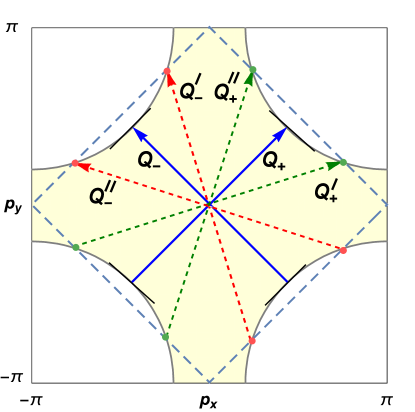
Figure 1: (Color online) The Fermi surface in the Brillouin zone for a nearly half-filled squared lattice Hubbard model, with two independent nesting vectors $Q_{\pm}$ defined in the text.

In the general case of a doped system vectors ${\bf Q}_{\pm}$ differ from half-filled nesting vectors $\{\pi,\pm\pi\}$ in the reciprocal cell units, and become independent, so we rewrite $(-1)^{x_{i}+y_{i}}m({\bf r}_{i})$ as

$$m_{+}({\bf r}_{i})\exp(i{\bf Q}_{+}{\bf r}_{+})+m_{-}({\bf r}_{i})\exp(i{\bf Q}_{-}{\bf r}_{-})+h.c.$$

Note, that we consider for simplicity a two pairs of almost plane sections of the Fermi surface with one pair of nesting vectors ${\bf Q}_{\pm}$ (See Fig. 1). In real systems there are two pairs of nesting vectors ${\bf Q}^{\prime}_{\pm}$ (shown in Figure), and ${\bf Q}^{\prime\prime}_{\pm}$, connecting opposite ”hotspots”.

In the continuous approximation eigenvalue equations take the form: $\hat{H}\Psi=\epsilon\Psi$, with

$$\hat{H}=\left(\matrix{-iV_{{\bf p}}\nabla_{{\bf r}}+\epsilon_{{\bf p}}-\eta&m_{\pm}({\bf r})&\Delta_{-{\bf p}}&0\cr m^{*}_{\pm}({\bf r})&-iV_{{\bf p}-{\bf Q}}\nabla_{{\bf r}}+\epsilon_{{\bf p}-{\bf Q}}-\eta&0&\Delta_{-({\bf p}-{\bf Q})}\cr\Delta_{{\bf p}}^{*}&0&iV_{{\bf p}}\nabla_{{\bf r}}-\epsilon_{{\bf p}}+\eta&m_{\pm}({\bf r})\cr 0&\Delta_{{\bf p}-{\bf Q}}^{*}&m^{*}_{\pm}({\bf r})&iV_{{\bf p}-{\bf Q}}\nabla_{{\bf r}}-\epsilon_{{\bf p}-{\bf Q}}+\eta}\right),$$ (6)

where $\eta=\eta({\bf r})=\mu-\frac{U}{2}\rho({\bf r})$, $\Psi^{T}=(u_{{\bf p}},u_{{\bf p}-{\bf Q}},v_{{\bf p}},v_{{\bf p}-{\bf Q}})=(u_{+},u_{-},v_{+},v_{-})$, $\epsilon_{{\bf p}}=-2t(\cos p_{x}+\cos p_{y})-\mu$, ${\bf V}_{{\bf p}}=2t(\sin p_{x},\sin p_{y})$. The vector ${\bf Q}={\bf Q}_{+}$ for ${\bf p}_{y}>0$, and ${\bf Q}={\bf Q}_{-}$ for $p_{y}<0$.

In the presence of the magnetic field ${\bf H}$ functions $u,v$ become spin-dependent, and equations (6) are changed: $\nabla\to\nabla-i\frac{e}{c}{\bf A}$, $\mu\to\mu_{\sigma}=\mu+\sigma\mu_{B}H$. For the constant magnetic field perpendicular to the plane we have ${\bf A}={\bf H}\times{\bf r}/2$, so that $\partial_{x}\to\partial_{x}+i(e/c)yH/2$, $\partial_{y}\to\partial_{y}-i(e/c)xH/2$. For the case $d_{x^{2}-y^{2}}$ symmetry we consider $\Delta_{-{\bf p}}=\Delta_{{\bf p}}=-\Delta_{{\bf p}-{\bf Q}}=2(\cos p_{x}-\cos p_{y})\Delta_{d}({\bf r})$.

The self-consistent conditions are derived by substitution of functions $u$, $v$ into (2). In the continuum approximation they read:

$$\rho({\bf r})=2\sum_{{\bf p}}[(u_{+}^{*}u_{+}+u_{-}^{*}u_{-})f+(v_{+}^{*}v_{+}+v_{-}^{*}v_{-})(1-f)]$$ (7)

$$(-1)^{x_{i}+y_{i}}m({\bf r})=4U[\sum_{{\bf p}}u_{-}^{*}u_{+}f-\sum_{{\bf p}}v_{-}^{*}v_{+}(1-f)]$$ (8)

$$\Delta_{\bf q}({\bf r})=2g\sum_{{\bf p}}(v_{+}^{*}u_{+}-v_{-}^{*}u_{-})[(1-f)(\cos(p_{x}-q_{x})$$

$$+\cos(p_{y}-q_{y}))-f((\cos(p_{x}+q_{x})+\cos(p_{y}+q_{y}))],$$ (9)

where $f={1}/({\exp[\epsilon_{{\bf p}}/T]+1})$. We omitted spin indices since in our representation for wave functions all equations are diagonal over spin.

III Superconductivity and spin-charge modulation

In the absence of superconductivity (low doping limit) the ground state is the periodic charge-spin superstructure with $\Delta_{d}=0$. Spins are ordered antiferromagnetically ($S_{z}\propto(-1)^{x+y}$) for the nondoped system ($\rho=1$). As a result of doping periodic structures of domain walls (stripe structure) are formed. Such solutions for the considered model were described earlier fe ; fe2 . Below we consider region of doping that allows a superconducting phase . In the general case a solution of the system of equations (6) is unknown. We present a solution taking into account both spin-charge and superconducting structure for a case of quasi-one-dimensional geometry, i.e. with broken fourfold rotational symmetry of the 2D-system.

There is a simplification for a pure superconducting state ($m({\bf r})=0$), where equations (6) are reduced to:

$$-i{\bf V}_{{\bf p}}\nabla_{{\bf r}}u_{{\bf p}}({\bf r})+\Delta_{{\bf p}}v_{{\bf p}}=\epsilon u_{{\bf p}}$$ (10)

$$\Delta_{{\bf p}}^{*}u_{{\bf p}}+i{\bf V}_{{\bf p}}\nabla_{{\bf r}}v_{{\bf p}}({\bf r})=\epsilon v_{{\bf p}}.$$ (11)

The term $U\rho({\bf r})/2$ in equations (6) can be eliminated by the shift of wave functions $u,v\to u,v\exp i\Phi$, ${\bf V_{p}}\nabla\Phi=U\rho({\bf r})/2$ sm ; mm . For filling factor $\rho\sim 1$, the Fermi surface has nearly square form, therefore ${\bf V}_{{\bf p}}\nabla_{{\bf r}}\approx V_{{\bf p}}\partial/\partial r_{\pm}$, depending on signs $p_{x},\,p_{y}$. The system of equations (10), (11) has the following vortex solution:

$$\Delta_{{\bf p}}({\bf r})=\Delta_{p}\frac{\sinh\frac{r_{+}}{\xi_{s}}+i\sinh\frac{r_{-}}{\xi_{s}}}{\sqrt{\sinh^{2}\frac{r_{+}}{\xi_{s}}+\sinh^{2}\frac{r_{-}}{\xi_{s}}+1}},$$ (12)

where $\Delta_{p}=\Delta_{d}(\cos(p_{x})-\cos(p_{y}))$; and $r_{\pm}=(x\pm y)/\sqrt{2}$. For $r_{-}=0$ the order parameter has a kink form $\Delta_{p}({\bf r})\propto\tanh r_{+}/\xi_{s}$, where superconducting correlation length $\xi_{s}$ has to be determined by minimization of the kink’s energy: $\xi_{s}\sim\bar{V_{p}}/\Delta_{d}$, and $\bar{V_{p}}$ is velocity averaged over the Fermi-surface.

For the case $r_{+}=0$ the order parameter acquires the phase: $\Delta_{p}({\bf r})\propto\exp(i\pi/2)\tanh r_{-}/\xi_{s}$. In the diagonal direction $r_{+}=r_{-}$ the solution $\Delta_{p}({\bf r})\propto\exp(i\pi/4)\tanh(r_{+}/\xi_{s})/\sqrt{\tanh^{2}r_{+}/\xi_{s}+1}$ has the phase $\pi/4$. It is known that in one-dimensional case finite-band solutions of equations (10) - (11) are related to the soliton (kink) solutions of the nonlinear Schrodinger equation (NSE). Note, that along the curve $\sinh r_{-}/\xi_{s}=\alpha\cosh r_{+}/\xi_{s}$ the order parameter acquires the form of a general kink solution of the NES: $\Delta_{p}({\bf r})\sim(i\alpha+\tanh x/\xi_{s})/\sqrt{\alpha^{2}+1}$ with the localized state in the gap with the energy $E_{0}=\Delta_{p}\alpha/\sqrt{\alpha^{2}+1}$. We suppose here that the magnetic field is small $H\ll H_{c_{2}}$, ($\xi_{s}\ll\lambda$, $\lambda$ is magnetic penetration depth), and therefore ignore the effect of terms with vector-potential on the solution at distances $r\ll\lambda$. The vortex structure (amplitude and phase) are shown in Fig. 2.

Figure 2: (Color online) The superconducting vortex solution Eq. (12) with contours of constant phase and modulus of the complex superconducting order parameter $\Delta_{p}(\vec{r})$.

For quasi-1D structures we can use the ansatz ma

$$v_{\pm}=\gamma_{\pm}u_{\mp}.$$

Considering $\epsilon({\bf p})-\mu=0$ on the Fermi surface we obtain for the case

$$m({\bf r})=|m({\bf r})|e^{i\varphi},\,\Delta_{{\bf p}}({\bf r})=|\Delta_{{\bf p}}({\bf r})|e^{i\varphi_{s}},\,\varphi,\,\varphi_{s}=const,$$

the solution $\gamma_{+}=\pm ie^{i(\varphi-\varphi_{s})},\,\gamma_{-}=\pm ie^{-i(\varphi+\varphi_{s})}$. Equations (6) are reduced to

$$-i{\bf V}_{{\bf p}}\nabla u_{+}+\tilde{\Delta}({\bf r})u_{-}=Eu_{+}$$ (13)

$$\tilde{\Delta}^{*}({\bf r})u_{+}+i{\bf V}_{{\bf p}}\nabla u_{-}=Eu_{-}$$ (14)

with function $\tilde{\Delta}({\bf r})=(|m({\bf r})|\pm i|\Delta_{{\bf p}}|)e^{i\varphi}$, and $m=m_{\pm}$, depending on the sign of $p_{y}$. Equations (13), (14) are exact provided that phases $\varphi$, $\varphi_{s}$ are constant or slowly varying in space functions. We show that inhomogeneity of the superconducting order parameter leads to the origination of the antiferromagnetic order parameter. Consider a 1D geometry case: $u=u(r_{+})$, where assumption of constant phases is valid. The solution of Eqs. (13), (14) describing the coexistence of superconductivity and spin-charge density ordering, compatible with self-consistent equations, has the form of two bound solitons of the nonlinear Schrodinger equation, see, for example, fadtakh

$$\tilde{\Delta}_{1,2}=\Delta_{p}\frac{\cosh(2\kappa x+c_{1})+\cosh(c_{2}\pm 2\beta i)/|\lambda|}{\cosh(2\kappa x+c_{1})+\cosh(c_{2})/|\lambda|},$$ (15)

where $E=\pm\lambda({\bf p})$ are positions of local levels inside the gap, $\kappa=\kappa_{p}=\sqrt{\Delta_{p}^{2}-\lambda^{2}}$, and $\exp i\beta=\lambda+i\kappa$. Eigenfunctions of equations (13), (14) have the form bm

$$u_{\pm}(x)\propto\sqrt{\tilde{\Delta}(x)(E^{2}-\gamma^{2}(x))}\exp\left[\pm i\int^{x}\frac{\sqrt{(E^{2}-\Delta_{p}^{2})(E^{2}-\lambda^{2})}}{E^{2}-\gamma^{2}(y)}dy\right],$$ (16)

where

$$\gamma(x)=\frac{1}{2}\frac{\partial}{\partial x}\ln\tilde{\Delta}(x).$$ (17)

The real and imaginary parts of (15) give superconducting and spin order parameters

$$\Delta_{sc}=\Delta_{p}(1-\Gamma\tanh a(\tanh(\frac{r_{+}}{\xi}+\frac{a}{2})-\tanh(\frac{r_{+}}{\xi}-\frac{a}{2}))),$$ (18)

$$m=m_{0}\Gamma\tanh a(\tanh(\frac{r_{+}}{\xi}+\frac{a}{2})-\tanh(\frac{r_{+}}{\xi}-\frac{a}{2})),$$ (19)

where we use a parametrization: $\Delta_{p}\sqrt{\Gamma_{p}}\tanh a=\kappa_{p}$, and $\Gamma_{p}=\Delta^{2}_{p}/(\Delta_{p}^{2}+m_{0}^{2})$. Averaged over Fermi surface functions are defined as: $\Gamma=<\Gamma_{p}>=<\Delta^{2}_{p}/(\Delta_{p}^{2}+m_{0}^{2})>_{p}$, $\xi=<v_{p}/(\Delta_{p}\sqrt{\Gamma_{p}}\tanh a)>_{p}$. Values of $m_{0}$, $\Delta_{{\bf p}}=\Delta_{d}(\cos p_{x}-\cos p_{y})$, $\xi$ and a dimensionless parameter $a$ are defined by the self-consistency conditions (8), (9); $m_{0}\propto t\times exp\{-t/U\}$ The solution describes the spin-charge stripe in superconducting phase (see Fig.3).

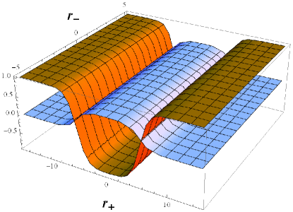
Figure 3: (Color online) Coexisting superconducting (downward) and antiferromagnetic stripe-like (upward) orders. The envelope functions from Eqs. (18), (19) are plotted in real space, $r_{-}$ and $r_{+}$ coordinates are measured in units of correlation length $\xi$, other parameters are: $a=7$, $\Delta_{d}=1$, $m_{0}=0.2$.

The spin inhomogeneity generates the charge distribution $\delta\rho({\bf r})\propto m^{2}({\bf r})$. Note, that two-soliton solution in the similar form was used for describing polaron-bipolaron states in the Peierls dielectrics brkir .

The superconducting correlation length is increased in comparison with clean superconductor case $\xi_{s}$ as $\xi=\xi_{s}\sqrt{1+\xi^{2}_{s}/\xi^{2}_{AF}}$, where the following definitions are assumed: $\xi_{s}=<v_{p}/\Delta_{p}>_{p}$, and $\xi_{AF}=<v_{p}/m_{0}>_{p}$.

The obtained structure is stabilized by applying a magnetic field. To show this we include the uniform magnetic field, perpendicular to the plane of the system. We will work in the limit of extreme type-II superconductivity (with Ginzburg-Landau parameter $\kappa=\lambda/\xi\to\infty$, $H_{c1}\sim\ln\kappa/\kappa\to 0$); so there is no screening of the magnetic field by the Meissner currents, and $\nabla\times{\bf A}=H\hat{\bf z}$, is an applied, space-independent magnetic field. In the symmetric gauge we have $A_{x}=-yH/2$, $A_{y}=xH/2$. In equations (13), (14) we substitute $-i\nabla\to-i\nabla-e{\bf A}/c$. The magnetic field can be excluded by transformation $u,v\to(u,v)\exp(ieHr_{+}r_{-}/2c)$.

The energy of the stripe structure (18), (19) in the magnetic field is given by

$$W=\sum E_{j}+\int d^{2}\\ r\left[\frac{\Delta_{d}^{2}}{g^{2}}+\frac{m^{2}}{g_{AF}^{2}}\right]-\int MHd^{2}r-W(a=0,m=0),$$ (20)

where

$$-\int MHd^{2}r=-\int m(r_{+})\cos(Qr_{+})Hdr_{+}=$$

$$-\frac{m_{0}\Gamma H\xi\tanh a}{\pi v_{p}\lambda}\frac{2\pi\sin(Q\xi a/2)}{\sinh(\pi Q\xi/2)}=-m_{0}H\frac{2}{\lambda\Delta_{p}}\sqrt{\Gamma}\frac{\sin\frac{Qv_{F}a}{2\sqrt{\Gamma}\Delta_{p}\tanh a}}{\sinh\frac{\pi Qv_{F}}{2\sqrt{\Gamma}\Delta_{p}\tanh a}},$$ (21)

$\xi=\xi_{0}/\tanh a$, $\xi_{0}=v_{F}/(\Delta_{p}\sqrt{\Gamma})$.

The first sum in (20) is found similar to brkir . After cumbersome calculations we obtain

$$W/L=\frac{4}{\pi}\Delta_{p}\left[\sqrt{\Gamma}\tanh a-\sqrt{1-\Gamma\tanh^{2}a}\,\arcsin[\sqrt{\Gamma}\tanh a]\right]+\frac{4}{\pi}m_{0}^{2}\frac{\sqrt{\Gamma}\tanh a}{\Delta_{p}\,\lambda}+$$

$$\frac{4}{\pi}m_{0}^{2}\frac{\Gamma^{3/2}}{\Delta_{p}}(a-\tanh a)\left(\frac{1}{\lambda_{AF}}-\frac{1}{\lambda}\right)-m_{0}H\frac{2}{\Delta_{p}\lambda}\sqrt{\Gamma}\frac{\sin\frac{Qv_{F}a}{2\sqrt{\Gamma}\Delta_{p}\tanh a}}{\sinh\frac{\pi Qv_{F}}{2\sqrt{\Gamma}\Delta_{p}\tanh a}},$$ (22)

where $\lambda=g^{2}/\pi v_{F}$. A typical dependence $W(a)$ is shown in Fig. 4

Figure 4: (Color online) The energy W(a) for magnetic fields $h=0$ (top curve), $h=0.5,0.8,1$ and $h=2$ (bottom curve)

The energy has a minimum with $W(a_{0})<0$ at $a_{0}\sim 1$ in a magnetic fields $\mu_{B}H\gtrsim m_{0}$ .

We conclude that in the region of inhomogeneity of superconducting order parameter a spin-density is formed. This coexisting structure is stabilized by applied magnetic field due to the fact, that $-\int MHd^{2}r$ in Eq.(21) over a finite-size AFM stripe is nonzero due to envelope shape suppression AFM spin variation close to the boundaries of the AFM stripe.

Note, that a similar solution can be written for the low-doping AFM spin-density wave region. The applied magnetic field stabilizes the stripe structure and results in generation of superconducting order parameter. Hence, the system possesses a kind of ’SO(5)’ symmetry.

IV Discussion

We considered a simple self-consistent 2D model on a squared lattice to describe different states, including charge-spin structures, superconductivity, and their coexistence. The origin of spin-charge periodic state (which is responsible for the pseudogap) is due to the existence of flat parallel segments of the Fermi surface (nesting) at low hole doping concentrations. Effects of commensurability lead to a pinning of stripe structure at rational filling points $|\rho-1|=m/n$. As a result, there is an exponentially small (for large $n$) decrease in the total energy of the order $\delta E\sim\exp(-c\,n)$ at any commensurate point, stabilizing stripes, as in 1D systems. For this reason, we think, stripes are mostly observable near $n=8$ point ($|\rho-1|=1/8$). An increase of doping leads to the decrease of flat segments of the Fermi surface and attenuation of spin-charge structure.

We found the solution describing the coexistence of superconductivity and stripes (18), (19). The decrease (or a deviation from the homogenous value) of the superconducting order parameter generates the spin-charge periodic structure in this region. Note, that due to symmetry of Eqs. (6),(13), (14) (duality $\Delta\leftrightarrow im$) we can write the same equation, describing the origin of superconducting correlations in the region of a inhomogeneity of spin-charge density. The situation is qualitatively similar to the 1D case ma . Experimental data in underdoped high-T_c cuprates LSCO aeppli1 indicates that antiferromagnetic stripe-like spin-density order can be induced by magnetic field perpendicular to the CuO planes in the interval of fields much smaller than upper critical field H_c2 . The size of the magnetically ordered domains exceeds superconducting vortex’s core size $\xi_{s}$ and the inter-vortex distance in the Abrikosov’s lattice. Our present theoretical results demonstrate that this is indeed possible in the simple Hubbard t-U-V model that we consider. In particular, the dimensionless parameter $a$ in Eqs. (18), (19) is an independent variational parameter and depends on the magnetic and superconducting coupling strengths ma , as well as on the magnitude of the external magnetic field. Hence, the size $\sim a\times\xi$ of the antiferromagnetic domain (see Fig. 3, upward bump) can exceed the superconducting (and magnetic) Ginzburg-Landau correlation length $\xi$ when $a(H)>>1$. Previously coexistence of superconducting order and slow antiferromagnetic fluctuations was studied merely on the basis of a phenomenological Ginzburg-Landau free energy functional approach in sachdev1 . We note also, that equations Eqs. (13), (14) can be simply extended to include d-density waves (DDW).
When this work was already done, we found a recent paper, in which authors efetov had provided theoretical description of the onset of charge ordered domain in the vortex core, where the superconducting order parameter turns to zero. This approach differs from ours in three major respects. The first one is that in efetov the absence of antiferromagnetic (AFM) order is assumed, while critical antiferromagnetic fluctuations are considered to provide coupling between electron-hole and Cooper channel fluctuations at the hot-spots and antipodal regions of the under-doped cuprates Fermi-surface, leading to a coexistence of superconducting (SC) and charge orders (CDW). The influence of an external magnetic field is considered in efetov merely as the prerequisite of CDW formation inside the superconducting cores. The second important respect of the difference with our approach is that the authors efetov consider an SU(2)-symmetric composite order parameter (CDW and SC), while we consider analytically a composite CDW-AFM-SC order parameter, since the AFM ’stripe’ coexisting with superconductivity incorporates CDW, AFM and SC orders. Finally, the third aspect of the difference is that the external magnetic field in our model couples to both the SC order and to finite-width stripe of AFM order. Unlike in the CDW-SC coexistence case in efetov , this leads to a two-fold stabilization of the stripe phase inside the superconducting cores: both by suppression of superconductivity and by dipole-like coupling of a net magnetic moment of a finite size AFM domains to magnetic field. Definitely, our model yet lacks all the versatile families of hot spot and antinodal nesting vectors (to be farther allowed for in the future), as considered in efetov , while so far we considered only two anti-ferromagnetic nesting wave-vectors instead.

V Acknowledgements

The work was carried out with financial support in part from the Ministry of Education and Science of the Russian Federation in the framework of Increase Competitiveness Program of NUST ”MISIS” (No. K2-2014-015) and from RFFI grant 12-02-01018.

References

- (1) Louis Taillefer, Annu. Rev. Condens Matter Phys. 1,51 (2010).
- (2) K. Jin, N.P. Butch, K. Kirshenbaum, J. Paglione and R.L. Greene, Nature 476, 73 (2011).
- (3) R. Daou et al., Nature 463, 519(2010).
- (4) B. Lake et al., Nature 415, 299 (2002).
- (5) A. T. Savici, et al., Physica B 289-290, 338 (2000).
- (6) Daniel Knapp, Catherine Kallin, Amit Ghosal and Sarah Mansour, Phys. Rev. B 71, 064504 (2005).
- (7) M. Einenkel, H. Meier, C. Pepin, and K. B. Efetov, Phys. Rev. B 90, 054511 (2014).
- (8) J. Zaanen and O. Gunnarsson, Phys. Rev. B 40, 7391 (1989).
- (9) M. Fujita, H. Goka, K. Yamada, J. M. Tranquada, and L. P. Regnault, Phys. Rev.B 70, 104517 (2004).
- (10) N. Ichikawa, S. Uchida, J. M. Tranquada, T. Niemöller, P. M. Gehring, S.-H. Lee, and J. R. Schneider, Phys. Rev. Lett. 85, 1738 (2000).
- (11) V. Hücker, M. v.Zimmermann, G. D. Gu, Z. J. Xu, J. S. Wen, Guangyong Xu, H. J. Kang, A. Zheludev, and J. M. Tranquada, Phys. Rev. B 83, 104506 (2011).
- (12) S. I. Mukhin, Phys. Rev. B 62, 4332 (2000).
- (13) S. I. Matveenko, S. I. Mukhin, Phys. Rev. lett. 84, 6066 (2000).
- (14) T. Valla, A.V. Federov, J. Lee, J. C. Davis, and G. D. Gu, Science 314, 1914 (2006).
- (15) B. Lake et al. Science 291, 1759 (2001).
- (16) J.E. Hoffman, E.W. Hudson, K.M. Lang, V. Madhavan, S.H. Pan, H. Eisaki, S. Uchida, and J.C. Davis, Science 295, 466 (2002).
- (17) V.F. Mitrovic., E.E. Sigmund, H.N. Bachman, M. Eschrig, W.P. Halperin, A.P. Reyes, P. Kuhns, and W.G. Moulton, Nature 413, 501 (2001).
- (18) S.-C. Zhang, Science 275, 1089 (1997).
- (19) Daniel P. Arovas, A.J. Berlinsky, C. Kallin, and Shou-Cheng Zhang, Phys. Rev. Lett. 79, 2871 (1997).
- (20) E. Demler, S. Sachdev and Y. Zhang, Phys. Rev. Lett. 87, 067202 (2001).
- (21) K. Park, S. Sachdev, Phys. Rev. B 64, 184510 (2001).
- (22) Y. Zhang, E. Demler and S. Sachdev, Phys. Rev. B 66, 094501 (2002).
- (23) G. E. Volovik, JETP Lett. 58, 469 (1993); P.I. Soininen, C. Kallin, A.J. Berlinsky, Phys. Rev. B 50, 13883 (1994); Y. Wang, A. H. MacDonald, Phys. Rev. B 52, R3876 (1995); M. Ichioka, N. Hayashi, N. Enomoto, and K. Machida, Phys. Rev. B 53, 15316 (1996); M. Franz, Z. Tesanovic, Phys. Rev. Lett. 80, 4763 (1998).
- (24) S. I. Mukhin, S. I. Matveenko, Int. Journ. Mod. Phys. B 17, 3749 (2003).
- (25) S. I. Matveenko, JETP Lett. 78, 384 (2003).
- (26) S. I. Matveenko, Int. Journ. Mod. Phys. B 23, 4297 (2009).
- (27) S. I. Matveenko, S. I. Mukhin, F. V. Kusmartsev, arXiv:1111.4139 [cond-mat.supr-con]
- (28) P.- G. de Gennes, Superconductivity of Metals and Alloys, Adison-Wesley Publ. Comp., 1966.
- (29) H. J. Schulz, J. Phys. (Paris) 50, 2833 (1989); Phys. Rev. Lett. 64, 1445 (1990).
- (30) L. D. Faddeev and L. A. Takhtajan, Hamiltonian Methods in the Theory of Solitons, Springer, Berlin (1987).
- (31) S. A. Brazovskii and S. I. Matveenko, Sov.Phys.JETP 60, 804 (1984).
- (32) S. A. Brazovskii and N. N. Kirova, JETP Lett. 33, 4 (1981).