Comparing different muscle activation dynamics using sensitivity analysis

Abstract

In this paper, we mathematically compared two models of mammalian striated muscle activation dynamics proposed by Hatze [8] and Zajac [27]. Both models are representative of a broad variety of biomechanical models formulated as ordinary differential equations (ODEs). The models incorporate some parameters that directly represent known physiological properties. Other parameters have been introduced to reproduce empirical observations. We used sensitivity analysis as a mathematical tool for investigating the influence of model parameters on the solution of the ODEs. That is, we adopted a former approach [16] for calculating such (first order) sensitivities. Additionally, we expanded it to treating initial conditions as parameters and to calculating second order sensitivities. The latter quantify the non-linearly coupled effect of any combination of two parameters. As a completion we used a global sensitivity analysis approach from Chan et al. [2] to take the variability of parameters into account. The method we suggest has numerous uses. A theoretician striving for model reduction may use it for identifying particularly low sensitivities to detect superfluous parameters. An experimenter may use it for identifying particularly high sensitivities to facilitate determining the parameter value with maximised precision.

We found that, in comparison to Zajac’s linear model, Hatze’s non-linear model incorporates a set of parameters to which activation dynamics is clearly more sensitive. Other than Zajac’s model, Hatze’s model can moreover reproduce measured shifts in optimal muscle length with varied muscle activity. Accordingly, we extracted a specific parameter set for Hatze’s model that combines best with a particular muscle force-length relation. We also give an outlook on how sensitivity analysis could be used for optimising parameter sets in future work.

List of symbols

Symbol	Meaning	Value
${\ell}_{CE}$	contractile element (CE) length	time-depending
$\dot{\ell}_{CE}$	contraction velocity	first time derivative of ${\ell}_{CE}$
${\ell}_{CEopt}$	optimal CE length	muscle-specific
${\ell}_{CErel}$	relative CE length	$\ell_{CErel}=\frac{{\ell}_{CE}}{{\ell}_{CEopt}}$ (dimensionless)
$F_{max}$	maximum isometric force of the CE	muscle-specific
$\sigma$	neural muscle stimulation	time-depending ; here: a fixed parameter
$q$	muscle activity (bound $Ca^{2+}$-concentration)	time-depending
$q_{0}$	basic activity according to Hatze [10]	$0.005$
$q_{H}$	activity according to Hatze [8]	time-length-depending
$q_{H,0}$	initial condition for Hatze’s activation ODE	mutable
$q_{Z}$	activity according to Zajac [27]	time-depending
$q_{Z,0}$	initial condition for Zajac’s activation ODE	mutable
$\tau$	activation time constant in Zajac [27]	here: $\frac{1}{40}\,s$
$\tau_{deact}$	deactivation time constant in Zajac [27]	here: $\frac{1}{40}\,s$ or $\frac{3}{40}\,s$
$\beta$	corresponding deactivation boost [27]	$\beta=\tau/\tau_{deact}$
$\nu$	exponent in Hatze’s formulation	2 or 3
$m$	activation frequency constant in Hatze [8]	range: $3.67\ldots 11.25\,\frac{1}{s}$ ; here: $10\frac{1}{s}$
$c$	maximal $Ca^{2+}$-concentration in Hatze [9]	$1.37\cdot 10^{-4}\,\frac{mol}{l}$
$\gamma$	representation of free $Ca^{2+}$-concentration [8, 10]	time-depending
$\rho$	length dependency of Hatze [9] activation dynamics	$\rho({\ell}_{CErel})=\rho_{c}\cdot\frac{{\ell}_{\rho}-1}{\frac{{\ell}_{\rho}}{{\ell}_{CErel}}-1}$
$\ell_{\rho}$	pole in Hatze’s length dependency function	$2.9$
$\rho_{0}$	factor in van Soest [24], Hatze [8]	$6.62\cdot 10^{4}\,\frac{l}{mol}$ ($\nu=2$) or $5.27\cdot 10^{4}\,\frac{l}{mol}$ ($\nu=3$)
$\rho_{c}$	merging of $\rho_{0}$ and $c$	$\rho_{c}=\rho_{0}\cdot c$ ; here: $9.10$ ($\nu=2$) or $7.24$ ($\nu=3$)
$\Lambda$	model parameter set	$\Lambda=\{\lambda_{1},\ldots,\lambda_{n}\}$

1 Introduction

In science, knowledge is gained by an interplay between quantitative real world measurements of physical, chemical, or biological phenomena and the development of mathematical models accounting for the dynamical processes behind. In general, such phenomena are determined as spatio-temporal patterns of physical measures (state variables). Modelling consists of distinguishing the surrounding world from a system that yields the phenomena, and formulating a mathematical description of the system, a model, that can calculate its state variables. The calculations depend on model parameters and often on prescribing measured input variables. By changing parameter values and analysing the resulting changes in the values of the state variables, the model may then be used as a predictive tool. This way, the model’s validity can be verified. If the mathematical model description is moreover derived from first principles, the model can potentially even explain the phenomena in a causal sense.

Calculating the sensitivities of a model’s predicted output, i.e., the system’s state variables, with respect to model parameters is a means of eliminating redundancy and indeterminancy from models, and thus helps to identify valid models. Sensitivity analyses can be helpful both in model-based experimental approaches and in purely theoretical work. A modelling theoretician may be looking for parameters to which all state variables are non-sensitive. Such parameters may be superfluous. An experimenter may inspect the model that represents his working hypothesis and analyse which of the model’s state variables are specifically sensitive to a selected parameter. It would then make sense to measure exactly this state variable to identify the value of the selected parameter.

In a biomechanical study, Scovil and Ronsky [21] applied sensitivity analysis to examine the dynamics of a mechanical multi-body system (a runner’s skeleton) coupled to muscle activation-contraction dynamics. They calculated specific sensitivity coefficients in three slightly different ways. A sensitivity coefficient is the difference quotient that is calculated from dividing the change in a state variable by the change in a model parameter value, evaluated in a selected system state [16]. The corresponding partial derivative may be simply called “sensitivity”. A sensitivity function is then the time evolution of a sensitivity [16]. Thus, Lehman and Stark [16] had proposed a more general and unified approach than Scovil and Ronsky [21], which allows to systematically calculate the sensitivities of any dynamical system described in terms of ordinary differential equations. As an example for sensitivity functions, Lehman and Stark [16] had applied their proposed method to a muscle-driven model of saccadic eye movement. By calculating a percentage change in a state variable value per percentage change in a parameter value, all sensitivities can be made comprehensively comparable, even across models. A sensitivity as defined so far is of first order. Methodically, we aim at introducing a step beyond, namely at calculating second order sensitivities. These measures are suited to quantifying how much the sensitivity of a state variable with respect to (w.r.t.) one model parameter depends on changing another parameter. This way, the strength of their interdependent influence on model dynamics can be determined.

In addition to this so-called local sensitivity analysis we furthermore take the variability of the parameters into account aiming for a global sensitivity analysis as presented in Chan et al. [2] and Saltelli [19]. This approach allows to translate sensitivities with respect to parameters into importances of parameters.

In this study, we will apply the sensitivity analysis to models that predict how the activity of a muscle (its chemical state) changes when the muscle is stimulated by neural signals (electrical excitation). Such models are used for simulations of muscles’ contractions coupled to their activation dynamics. Models for coupled muscular dynamics are often part of neuro-musculo-skeletal models of biological movement systems. In particular, we want to try and rate two specific model variants of activation dynamics formulated by Zajac [27] and by Hatze [8]. As a first result, we present an example of a simplified version of the Zajac [27] model, in which sensitivity functions can even be calculated in closed form. Then, we calculate the sensitivities numerically with respect to all model parameters in both models, aiming at an increased understanding of the influence of changes in model parameters on the solutions of the underlying ordinary differential equations (ODEs). Additionally, we discuss which of both models may be the more physiological one. The arguments come from a mixture of three different aspects: sensitivity analysis, others’ experimental findings, and an additional attempt to best fit different combinations of activation dynamics and force-length relations of the contractile element (CE) in a muscle to known data on shifts in optimal CE length with muscle activity [11].

2 Two models for muscle activation dynamics

Macroscopically, a muscle fibre or an assembly of muscle fibres (muscle belly) is often mapped mathematically by a one-dimensional massless thread called “contractile component” or “contractile element” (CE) [24, 25, 3, 6, 7]. Its absolute length is ${\ell}_{CE}$ which may be normalised to the optimal fibre length ${\ell}_{CEopt}$ by ${\ell}_{CErel}={\ell}_{CE}/{\ell}_{CEopt}$. In macroscopic muscle models, the CE muscle force is usually modelled as a function of a force-(CE-)length relation, a force-(CE-)velocity relation, and (CE-)activity $q$. A common view is that muscle activity $q$ represents the number of attached cross-bridges within the muscle, normalised to the maximum number available ($q_{0}\leq q\leq 1$). It can also be considered as the concentration of bound Ca²⁺-ions in the muscle sarcoplasma relative to its physiological maximum. The parameter $q_{0}$ represents the minimum activity that is assumed to occur without any stimulation [8].

We analyse two different formulations of muscle activation dynamics, i.e., the time (its symbol: $t$) evolution of muscle activity $q(t)$. One formulation of muscle activation dynamics was suggested by Zajac [27] which we modified slightly to take $q_{0}$ into account:

$$\dot{q}_{Z}=\frac{1}{\tau\cdot(1-q_{0})}\cdot\left[\sigma\cdot(1-q_{0})-\sigma\cdot(1-\beta)\cdot(q_{Z}-q_{0})-\beta\cdot(q_{Z}-q_{0})\right],\quad q_{Z}(0)=q_{Z,0}\quad.$$ (1)

Here, $\sigma$ is meant to represent the (electrical) stimulation of the muscle, thus, a parameter for controlling muscle dynamics. It represents the output of the nervous system’s dynamics applied to the muscle which in turn interacts with the skeleton, the body mass distribution, the external environment, and so with the nervous system in a feedback loop. Electromyographic (EMG) signals can be seen as a compound of such neural stimulations collected in a finite volume (being the input to a number of muscle fibres), over a frequency range, and coming from a number of (moto-)neurons. The parameter $\tau$ denotes the activation time constant, and $\beta=\tau/\tau_{deact}$ is the ratio of activation to deactivation time constants (deactivation boost).

An alternative formulation of muscle activation dynamics was introduced by Hatze [8]:

$$\dot{\gamma}=m\cdot(\sigma-\gamma)\quad.$$ (2)

Here, we divided the original equation from Hatze [8] by the parameter $c=1.37\cdot 10^{-4}\,\frac{mol}{l}$ which represents the maximum concentration of free Ca²⁺-ions in the muscle sarcoplasma. Thus, the values of the corresponding normalised concentration are $0\leq\gamma\leq 1$. The activity is then finally calculated by the function

$$q_{H}(\gamma,{\ell}_{CErel})=\frac{q_{0}+[\rho({\ell}_{CErel})\cdot\gamma]^{\nu}}{1+[\rho({\ell}_{CErel})\cdot\gamma]^{\nu}}\quad,$$ (3)

and the parameter $c$ is shifted to the accordingly renormalised function

$$\rho({\ell}_{CErel})=\rho_{c}\cdot\frac{{\ell}_{\rho}-1}{\frac{\ell_{\rho}}{{\ell}_{CErel}}-1}\quad,$$ (4)

with $\rho_{c}=c\cdot{\rho}_{0}$ and ${\ell}_{\rho}=2.9$. Two cases have been suggested by Hatze [10]: ${\rho}_{0}=6.62\cdot 10^{4}\,\frac{l}{mol}$ (i.e. $\rho_{c}=9.10$) for $\nu=2$ and ${\rho}_{0}=5.27\cdot 10^{4}\,\frac{l}{mol}$ (i.e. $\rho_{c}=7.24$) for $\nu=3$ which has been applied in literature [24, 11, 12, 13]. By substituting equations (2) and (3) into $\dot{q_{H}}=\frac{dq_{H}(\gamma,{\ell}_{CErel})}{d\gamma}\cdot\dot{\gamma}$ and resubstituting the inverse of (3) afterwards, Hatze’s formulation of an activation dynamics can be transformed into a non-linear differential equation directly in terms of the activity:

$$\dot{q}_{H}=\frac{\nu\cdot m}{1-q_{0}}\cdot\left[\sigma\cdot\rho({\ell}_{CErel})\cdot(1-q_{H})^{1+1/\nu}\cdot(q_{H}-q_{0})^{1-1/\nu}-(1-q_{H})\cdot(q_{H}-q_{0})\right]\;,\qquad\;$$ (5)

with initial condition $q_{H}(0)=q_{H,0}$.

The solutions $q_{Z}(t)$ and $q_{H}(t)$ of both formulations of activation dynamics (1) and (5), respectively, can now be directly compared by integrating them with the same initial condition $q_{Z}(t=0)=q_{H}(t=0)$ using the same stimulation $\sigma$.

3 Local first and second order sensitivity of ODE systems regarding their parameters

Let $\Omega\subseteq\mathbb{R}\times\mathbb{R}^{M}\times\mathbb{R}^{N}$ and $f:\,\Omega\rightarrow\mathbb{R}^{M}$. We then consider a system of ordinary, first order initial value problems (IVP)

$$\dot{Y}=f(t,Y(t,\Lambda),\Lambda)\quad,\qquad Y(0)=Y_{0}\quad,$$ (6)

where $Y=(y_{1}(t),y_{2}(t),\ldots,y_{M}(t))$ denotes the vector of state variables, $f=(f_{1},f_{2},\ldots,f_{M})$ the vector of right-hand sides of the ODE, and $\Lambda=\{\lambda_{1},\lambda_{2},\ldots,\lambda_{N}\}$ the set of parameters which the ODE depends on. The vector of initial conditions is abbreviated by

$$Y(0)=(y_{1}(0),y_{2}(0),\ldots,y_{M}(0))=(y_{1,0},y_{2,0},\ldots,y_{M,0})=Y_{0}\quad.$$ (7)

Then, the first order solution sensitivity with respect to the parameter set $\Lambda$ is defined as the matrix

$$S(t,\Lambda)=(S_{ik}(t,\Lambda))_{i=1,\ldots,N,k=1,\ldots,M}\quad,\qquad\text{with}\qquad S_{ik}(t,\Lambda)=\frac{d}{d\lambda_{i}}y_{k}(t,\Lambda)\quad.$$ (8)

For simplicity, we denote $Y=Y(t,\Lambda)$, $f=f(t,Y,\Lambda)$, $S_{ik}=S_{ik}(t,\Lambda)$ but keep the dependencies in mind. Because the solution $Y(t)$ might only be gained numerically rather than in a closed-form expression, we have to apply the well-known theory of sensitivity analysis as stated in Vukobratovic [26], Gelinas [5], Lehman and Stark [16], ZivariPiran [28]. Differentiating equation (8) w.r.t. $t$ and applying the chain rule yields

$$\frac{d}{dt}S_{ik} =\frac{d^{2}}{dt\,d\lambda_{i}}y_{k}=\frac{d^{2}}{d\lambda_{i}\,dt}y_{k}=\frac{d}{d\lambda_{i}}f_{k}=\frac{d}{d\lambda_{i}}Y\cdot\frac{\partial}{\partial Y}f_{k}+\frac{\partial}{\partial\lambda_{i}}f_{k}\quad,$$

with $$\frac{\partial}{\partial Y}$$ being the gradient of state variables. Hence, we obtain the following ODE for the first order solution sensitivity

$$\dot{S}_{ik} =\sum\limits_{l=1}^{M}S_{il}\cdot\frac{\partial}{\partial y_{l}}f_{k}+\frac{\partial}{\partial\lambda_{i}}f_{k}\quad,\qquad S_{ik}(0)=\frac{\partial}{\partial\lambda_{i}}y_{k,0}=0\quad,$$ (9)

or in short terms

$$\dot{S}=S\cdot J+B\quad,\qquad S(0)=\mathbf{0}_{N\times M}\quad,$$

where $S=S(t)$ is the $N\times M$ sensitivity matrix, $J=J(t)$ is the $M\times M$ Jacobian matrix with $J_{kl}=\frac{\partial}{\partial y_{l}}f_{k}$, furthermore $B=B(t)$ the $N\times M$-matrix containing the partial derivatives $B_{ik}=\frac{\partial}{\partial\lambda_{i}}f_{k}$ and $\mathbf{0}_{N\times M}$ the $N\times M$-matrix consisting of zeros only.

By analogy, the second order sensitivity of $Y(t)$ with respect to $\Lambda$ is defined as the following $N\times N\times M$-tensor

$$R(t,\Lambda)=(R_{ijk}(t,\Lambda))_{i,j=1,\ldots N,k=1,\ldots M}\quad,$$

with

$$R_{ijk}(t,\Lambda)=\frac{d}{d\lambda_{i}}S_{jk}=\frac{d}{d\lambda_{j}}S_{ik}=\frac{d^{2}}{d\lambda_{i}\,d\lambda_{j}}y_{k}=R_{jik}(t,\Lambda)\quad,$$ (10)

assuming $R_{ijk}=R_{jik}$ for all $k=1,\ldots,M$. That is, we assume that the prerequisites of Schwarz’ Theorem (symmetry of the second derivatives) are fulfilled throughout. Again, differentiating w.r.t. $t$ and applying the chain rule leads to the ODE

$$\dot{R}_{ijk}=\sum\limits_{l=1}^{M}\left(R_{ijl}\frac{\partial}{\partial y_{l}}f_{k}+S_{il}\frac{\partial}{\partial\lambda_{j}}f_{k}+S_{jl}\frac{\partial}{\partial\lambda_{i}}f_{k}\right)+\sum\limits_{l_{1}=1}^{M}\sum\limits_{l_{2}=1}^{M}S_{il_{1}}S_{jl_{2}}\frac{\partial^{2}}{\partial y_{l_{1}}\partial y_{l_{2}}}f_{k}+\frac{\partial^{2}}{\partial\lambda_{i}\partial\lambda_{j}}f_{k}\quad,$$ (11)

with $R_{ijk}(0)=0$. For purposes beyond the aim of this paper, a condensed notation introducing the concept of tensor (or Kronecker) products as in ZivariPiran [28] may be helpful. For a practical implementation in MatLab see Kolda [14].

Furthermore, if an initial condition $y_{k,0}$ (see (7)) is considered as another parameter we can derive a separate sensitivity differential equation by rewriting equation (6) in its integral form

$$Y(t)=Y_{0}+\int\limits_{0}^{t}f(s,Y(s))\text{ d}s\quad.$$

Differentiating this equation w.r.t. $Y_{0}$ yields

$$S_{Y_{0}}(t)=\frac{\partial}{\partial Y_{0}}Y(t)=1+\int\limits_{0}^{t}\frac{\partial}{\partial Y}f\cdot\frac{\partial}{\partial Y_{0}}Y(s)\text{ d}s$$

and differentiating again w.r.t. $t$ results in a homogeneous ODE for each component $S_{y_{k,0}}(t)$, namely

$$\dot{S}_{y_{k,0}}(t)=\sum\limits_{l=1}^{M}\frac{\partial}{\partial y_{l}}f_{k}\cdot S_{y_{l,0}}\quad,\qquad\text{ with }\qquad S_{y_{k,0}}(0)=\frac{\partial}{\partial y_{k,0}}y_{k,0}=1\quad.$$ (12)

The parameters of our analysed models are meant to represent physiological processes, and bear physical dimensions therefore. For example, $m$ and $\frac{1}{\tau}$ are frequencies measured in [Hz], whereas $c$ is measured in [mol/l]. Accordingly, $S_{\tau}=\frac{d}{d\tau}q_{Z}$ would be measured in [Hz] and $S_{m}$ in [s] (note that our model only consists of $one$ ODE and therefore we do not need a second index). Normalisation provides a comprehensive comparison between all sensitivities, even across models. For any parameter, the value $\lambda_{i}$ fixed for a specific simulation is a natural choice. For any state variable, we chose its current value $y_{k}(t)$ at each point in time of the corresponding ODE solution. Hence, we normalise each sensitivity $S_{ik}=\frac{dy_{k}}{d\lambda_{i}}$ by multiplying it with the ratio $\frac{\lambda_{i}}{y_{k}(t)}$ to get the relative sensitivity

$$\tilde{S}_{ik}=S_{ik}\cdot\frac{\lambda_{i}}{y_{k}}\quad.$$ (13)

A relative sensitivity $\tilde{S}_{ik}$ thus quantifies the percentage change in the $k$-th state variable value per percentage change in the $i$-th parameter value. This applies accordingly to the second order sensitivity

$$\tilde{R}_{ijk}=R_{ijk}\cdot\frac{\lambda_{i}\cdot\lambda_{j}}{y_{k}}\quad.$$ (14)

It can be shown that this method is valid and mathematically equivalent to another common method in which the whole model is non-dimensionalised a priori [20]. A non-normalised model formulation has the additional advantage of usually allowing a more immediate appreciation of and transparent access for experimenters. In the remainder of this manuscript, we always present and discuss relative sensitivity values normalised that way.

In our model, the specific case $M=1$ applies, so equations (9) and (11) simplify to the case $k=1$ (no summation).

4 Variance-based global sensitivity analysis

The previous presented differential sensitivity analysis is called a local method because it does not take the physiological range of parameter values into account. If we imagine the parameter space as a $N$-dimensional cuboid $\mathcal{C}=[\lambda_{1}^{-};\lambda_{1}^{+}]\times\ldots\times[\lambda_{N}^{-};\lambda_{N}^{+}]$, where $\lambda_{i}^{-},\lambda_{i}^{+}$ are the minimal and maximal parameter value, we can only fix a certain point $\hat{\Lambda}=(\hat{\lambda}_{1},\ldots,\hat{\lambda}_{N})\in\mathcal{C}$ and calculate the local gradient of the solution w.r.t. $\hat{\Lambda}$. By changing only one parameter at once the investigated star-shaped area lies within a ball around $\hat{\Lambda}$ whose volume vanishes in comparison to $\mathcal{C}$ for an increasing number of parameters as shown in Saltelli and Annoni [18].

For taking the range of parameter values into account, Saltelli [19] gave a detailed elaboration of so-called global methods. The main idea behind most global methods is to include a statistical component to scan the whole parameter space $\mathcal{C}$ and combine the percentage change of the state variable per percentage change of the parameters with the variability of the parameters themselves. For an overview of the numerous methods like ANOVA, FAST, Regression or Sobol’ Indexing we refer the reader to Saltelli [19] and Frey [4].

In this paper we want to sketch the main idea of the variance-based sensitivity analysis approach presented in Chan et al. [2] based on Sobol’ indexing. We chose this method because of its transparency and low computational cost. The aim of this method is to calculate two measurands of sensitivity w.r.t. parameter $\lambda_{i}$: the variance based sensitivity function denoted by $VBS_{i}(t)$ and the total sensitivity index function denoted by $TSI_{i}(t)$. The $VBS$ functions give a normalised first order sensitivity quite similar to $\tilde{S}$ from the previous section but include the parameter range. The $TSI$ functions, however, even include higher order sensitivities and give a measurand for interactions of parameter influences.

A receipt for calculating $VBS$ and $TSI$ can be given as follows. First of all set boundaries for all model parameters, either by model assumptions or literature reference, thus by resulting in $\mathcal{C}$. Secondly generate two sets of $n$ sample points $\hat{\Lambda}_{1,j},\hat{\Lambda}_{2,j}\in\mathcal{C},\;j=1,..,n$ w.r.t to the underlying probability distribution of each parameter, in our case the uniform distribution. Thirdly calculate $2nN$ sets of new sample points $\hat{\Lambda}_{1,j}^{i},\hat{\Lambda}_{1,j}^{\sim i},\;j=1,..,n,\;i=1,..,N$ where $\hat{\Lambda}_{1,j}^{i}$ consists of all sample points in $\hat{\Lambda}_{1,j}$ with the $i$-th component of $\hat{\Lambda}_{2,j}$. Consequently $\hat{\Lambda}_{1,j}^{\sim i}$ consists of the $i$-th component of $\hat{\Lambda}_{1,j}$ and every other component of $\hat{\Lambda}_{2,j}$. Fourthly evaluate the model from Eqn. (6) on every of the $2n(N+1)$ sample points $\hat{\Lambda}_{1,j},\hat{\Lambda}_{2,j},\hat{\Lambda}_{1,j}^{i},\hat{\Lambda}_{1,j}^{\sim i}$ resulting in a family of solutions. For this family perform the following calculations:

1. Compute the variance of the family of all $2n(N+1)$ solutions as a function of time, namely $V(t)$. This variance function indicates the general model output variety throughout the whole parameter range.

2. Compute the variance of the family of all $nN+1$ solutions resulting from an evaluation of the model at $\hat{\Lambda}_{1,j}$ and $\hat{\Lambda}_{1,j}^{i}$. Again the variance is a function of time, namely $V_{i}(t)$, that indicates the model output variety if only one parameter value is changed.

3. Compute the variance of the family of all $nN+1$ solutions resulting from an evaluation of the model at $\hat{\Lambda}_{1,j}$ and $\hat{\Lambda}_{1,j}^{\sim i}$, namely $V_{\sim i}(t)$, that indicates the model output variety if only one parameter value fixed.

Note that in Chan et al. [2] the coputations are done via an approximation by Monte-Carlo integrals. The $VBS$ and $TSI$ can finally be calculated as

$$VBS_{i}(t)=\frac{V_{i}(t)}{V(t)},\qquad TSI_{i}=1-\frac{V_{\sim i}(t)}{V(t)}$$ (15)

As a consequence of the normalisation we can give additional properties of $VBS$ and $TSI$ that can be comprehended in [2, Fig. 1]:

$$\sum\limits_{i=1}^{N}VBS_{i}(t)\leq 1,\qquad\sum\limits_{i=1}^{N}TSI_{i}(t)\geq 1$$ (16)

In other words $VBS_{i}(t)$ gives the normalised first order sensitivity function of the solution w.r.t. $\lambda_{i}$ in relation to the model output range. Accordingly $TSI_{i}(t)$ gives a relative influence of parameter $\lambda_{i}$ on the model output regarding all interactions between other parameters. Chan et al. [2] suggested relating the $TSI_{i}(t)$ value to the “importance” of $\lambda_{i}$.

5 An analytical example for local sensitivity analysis including a link between Zajac’s and Hatze’s formulations

By further simplifying Zajac’s formulation of an activation dynamics (1) through assuming an deactivation boost $\beta=1$ (activation and deactivation time constants are equal) and a basic activity $q_{0}=0$, we obtain a linear ODE for this specific case $q_{Z}^{sp}$ which is equivalent to Hatze’s equation (2) modelling the time evolution of the free Ca²⁺-ion concentration:

$$\dot{q}_{Z}^{sp}=\frac{1}{\tau}(\sigma-q_{Z}^{sp})\quad,\qquad q_{Z}^{sp}(0)=q_{Z,0}\quad.$$ (17)

By analysing this specific case, we aim at making the above described sensitivity analysis method more transparent for the reader. Solving equation (17) yields

$$q_{Z}^{sp}(t)=\sigma\cdot(1-e^{-t/\tau})+q_{Z,0}\cdot e^{-t/\tau}$$ (18)

depending on just two parameters $\sigma$ (stimulation: control parameter) and $\tau$ (time constant of activation: internal parameter) in addition to the initial value $y_{0}=q_{Z,0}$. The solution $q_{Z}(t)$ equals the $\sigma$ value after about $\tau$.

Although already knowing the solution (18) explicitly in terms of time and both parameters, we still apply, because of transparency, the more generally applicable, implicit method (9),(12) to determine the derivatives of the solution w.r.t. the parameters (the sensitivities). For that, we calculate the gradient of the right hand side $f(q_{Z}^{sp},\sigma,\tau)$ of the ODE (17)

$$\frac{\partial}{\partial q_{Z}^{sp}}f=-\frac{1}{\tau}\quad,\quad\frac{\partial}{\partial\sigma}f=\frac{1}{\tau}\quad,\text{and}\quad\frac{\partial}{\partial\tau}f=-\frac{\sigma-q_{Z}^{sp}}{\tau^{2}}=\frac{q_{Z,0}-\sigma}{\tau^{2}}e^{-t/\tau}$$

and insert these partial derivatives into equations (9) and (12). Solving the respective three ODEs for the three parameters ($\sigma,\tau$, $q_{Z,0}$) and normalising them according to (13) gives the relative sensitivities of $q_{Z}^{sp}$ w.r.t. $\sigma$, $\tau$, and $q_{Z,0}$ as functions of time (see Fig. 1):

$$\tilde{S}_{\sigma}(t)=(1-e^{-t/\tau})\cdot\frac{\sigma}{q_{Z}^{sp}(t)}=\frac{\sigma\cdot(e^{t/\tau}-1)}{\sigma\cdot(e^{t/\tau}-1)+q_{Z,0}}\quad,$$ (19)

$$\tilde{S}_{\tau}(t)=\left(\frac{(q_{Z,0}-\sigma)\cdot t}{\tau^{2}}e^{-t/\tau}\right)\cdot\frac{\tau}{q_{Z}^{sp}(t)}=\frac{t\cdot(q_{Z,0}-\sigma)}{\tau\cdot[\sigma\cdot(e^{t/\tau}-1)+q_{Z,0}]}\quad\text{, and}$$ (20)

$$\tilde{S}_{q_{Z,0}}(t)=e^{-t/\tau}\cdot\frac{q_{Z,0}}{q_{Z}^{sp}(t)}=\frac{q_{Z,0}}{\sigma\cdot(e^{t/\tau}-1)+q_{Z,0}}\quad.$$ (21)

A straight forward result is that the time constant $\tau$ has its maximum effect on the solution (Fig. 1: see $\tilde{S}_{\tau}(t)$) at time $t=\tau$. In case of a step in stimulation, the sensitivity $\tilde{S}_{\tau}(t)$ vanishes in the initial situation and exponentially approaches zero again after a few further times the typical period $\tau$. Note that $\tilde{S}_{\tau}(t)$ is negative which means that an increase in $\tau$ decelerates activation. That is, for a fixed initial value $q_{Z,0}$, the solution value $q_{Z}(t)$ decreases at a given point in time if $\tau$ is increased. After a step in stimulation $\sigma$, the time in which the solution $q_{Z}(t)$ bears some memory of its initial value $q_{Z,0}$ is equal to the period of being non-sensitive to any further step in $\sigma$ (compare $\tilde{S}_{q_{Z,0}}(t)$ to $\tilde{S}_{\sigma}(t)$ and (19) to (21)). After about $\tau/2$ the sensitivity $\tilde{S}_{q_{Z,0}}(t)$ has already fallen to about $0.1$ and $\tilde{S}_{\sigma}(t)$ to about $0.9$ accordingly.

Figure 1: Relative sensitivities $\tilde{S}_{i}$ w.r.t. the three parameters in the simplified formulation (17) of Zajac’s activation dynamics (1). Parameters: stimulation $\sigma$ (see (19): solid line), activation time-constant $\tau$ (see (20): dashed line), and initial activation $q_{Z,0}$ (see (21): dash-dotted line). Note that $\tilde{S}_{\tau}$ is negative, but for reasons of comparability we have plotted its absolute value. Parameter values are $\sigma=1$, $\tau=\frac{1}{40}\,s=0.025\,s$, and $q_{Z,0}=0.05$. Because the ODE (17) for $q_{Z}^{sp}$ is equivalent to Hatze’s ODE (2) for the free Ca²⁺-ion concentration, $\gamma$, we can identify the sensitivity of $\frac{1}{\tau}$ with that of $m$.

6 The numerical approach and results

Typically, biological dynamics are represented by non-linear ODEs. So the linear ODE used for describing activation dynamics in the Zajac [27] case (1) is more of an exception. For example, a closed-form solution can be given. (18) is an example as shown in the previous section for the reduced case of non-boosted deactivation (17).

In general, however, non-linear ODEs used in biomechanical modelling, as the Hatze [8] case (5) for describing activation dynamics, can only be solved numerically. It is understood that any explicit formulation of a model in terms of ODEs allows to provide the partial derivatives of their right hand sides $f$ w.r.t. the model parameters in a closed form. Fortunately, this is exactly what is required as part of the sensitivity analysis approach presented in section 3, in particular in equation (9).

As an application for applying this approach, we will now present a comparison of both formulations of activation dynamics. The example indicates that the approach may be of general value because it is common practice in biomechanical modelling to (i) formulate the ODEs in closed form and (ii) integrate the ODEs numerically. Adding further sensitivity ODEs for model parameters is then an inexpensive enhancement of the procedure used to solve the problem anyway.

For the two different activation dynamics [27] and [8], the parameter sets $\Lambda_{Z}$ and $\Lambda_{H}$, respectively, consist of

$$\Lambda_{Z} =\{\,q_{Z,0},\,\sigma,\,q_{0},\,\tau,\,\beta\,\}\quad,$$ (22)

$$\Lambda_{H} =\{\,q_{H,0},\,\sigma,\,q_{0},m,\,\rho_{c},\,\nu,\,\ell_{\rho},\,{\ell}_{CErel}\,\}\quad,$$ (23)

including the initial conditions. The numerical solutions for these ODEs were computed within the MATLAB environment (The MathWorks, Natick, USA; version R2013b) using the pre-implemented numerical solver $ode45$ which is a Runge-Kutta algorithm of order 5 (for details see [1]).

6.1 Results for Zajac’s activation dynamics: sensitivity functions

We simulated activation dynamics for the parameter set $\Lambda_{Z}$ (22) leaving two of the values constant ($q_{0}=0.005$, $\tau=\frac{1}{40}\,s$) and varying the other three (initial condition $q_{Z,0}$, stimulation $\sigma$, and deactivation boost $\beta$). The time courses of the relative sensitivities $\tilde{S}_{i}(t)$ w.r.t. all parameters $\lambda_{i}\in\Lambda_{Z}$ are plotted in Fig. 2. In the left column of Fig. 2, $\beta=1$ is used, in the right column $\beta=1/3$. Pairs of the parameter values $q_{0}=0.005\leq q_{Z,0}\leq 0.5$ and $0.01\leq\sigma\leq 1$ are specified in the legend of Fig. 2, with increasing values of both parameters from top to bottom.

Relative sensitivity $\tilde{S}_{q_{0}}$

Solutions are non-sensitive to the $q_{0}$ choice except if both initial activity and stimulation (also approximating the final activity if $\beta=1$ and $\sigma>>q_{0}$) are very low nearby $q_{0}$ itself.

Relative sensitivity $\tilde{S}_{q_{Z,0}}$

The memory (influence on solution) of the initial value is lost after about $2\tau$, almost independently of all other parameters. This loss in memory is obviously slower than in the extreme case $q_{Z,0}=0$ (initial value) and $\sigma=1$ (for $\beta=1$ and $q_{0}=0$ exactly the final value; see section 5 and Fig. 1). In that extreme case, the influence (relative sensitivity) of the lowest possible initial value ($q_{Z,0}=0$) on the most rapidly increasing solution (maximum possible final value: $\sigma=1$) is lost earlier.

Relative sensitivity $\tilde{S}_{\tau}$

The influence of the time constant $\tau$ on the solution is reduced with decreasing difference between initial and final activity values (compare maximum $\tilde{S}_{\tau}$ values in Figs. 1 and 2) and, no matter the $\beta$ value, with compoundly raised levels of initial activity $q_{Z,0}$ and $\sigma$, the latter determining the final activity value if $\beta=1$. When deactivation is slower than activation ($\beta<1$: right column in Fig. 2) $\tilde{S}_{\tau}$ is higher than in the case $\beta=1$, both in its maximum amplitude and for longer times after the step in stimulation, especially at low activity levels (upper rows in Fig. 2).

Relative sensitivity $\tilde{S}_{\sigma}$

Across all parameters, the solution is in general most sensitive to $\sigma$. However, the influence of the deactivation boost parameter $\beta$ is usually comparable. In some situations, this holds also for the activation time constant $\tau$ (see below). For $\beta=1$ (Fig. 2, left), the solution becomes a little less sensitive to $\sigma$ with decreasing activity level ($\tilde{S}_{\sigma}<1$), which reflects that the final solution value is not determined by $\sigma$ alone but by $q_{0}>0$ and $\beta\neq 1$ as much. If deactivation is much slower than activation ($\beta=\frac{1}{3}<1$: Fig. 2, right), we find the opposite to the case $\beta=1$: $\sigma$ determines the solution the less the more the activity level rises. Additionally, stimulation $\sigma$ somehow competes with both deactivation boost $\beta$ and time constant $\tau$ (see further below). Using the term “compete” is meant to illustrate the idea that any single parameter should have in a sense an individual interest in influencing the dynamics as much as possible in order not to be considered superfluous.

Relative sensitivity $\tilde{S}_{\beta}$

Sensitivity w.r.t $\beta$ generally decreases with increasing activity $q_{Z,0}$ and stimulation $\sigma$ levels, and vanishes at maximum stimulation $\sigma=1$.

Relative sensitivities $\tilde{S}_{\sigma}$, $\tilde{S}_{\beta}$, $\tilde{S}_{\tau}$

At submaximal stimulation levels $\sigma<1$, the final solution value is determined to almost the same degree by stimulation $\sigma$ and deactivation boost $\beta$, yet, with opposite tendencies ($\tilde{S}_{\sigma}>0$, $\tilde{S}_{\beta}<0$). Both parameters compete, in the above explained meaning, for their impact on the final solution value. Only at maximum stimulation $\sigma=1$ (lowest row in Fig. 2), this parameter competition is resolved in favour of $\sigma$. In this specific case, $\beta$ does not influence the solution at all. For $\beta=1$ the competition about influencing the solution is intermittently but only slightly biased by $\tau$: sensitivity $\tilde{S}_{\tau}$ peaks at comparably low magnitude around $t=\tau$. This $\tau$ influence comes likewise intermittently at the cost of $\beta$ influence: the absolute value of $\tilde{S}_{\beta}$ rises a little slower than $\tilde{S}_{\sigma}$. In the case $\beta<1$, this competition becomes even more differentiated and spreaded out in time. Again at submaximal stimulation and activity levels, the absolute value of $\tilde{S}_{\tau}$ is lower than that of $\tilde{S}_{\sigma}$ but higher than that of $\tilde{S}_{\beta}$, making all three parameters $\sigma$, $\beta$, and $\tau$ compete to comparable degrees for an impact on the solution until about $t=4\tau$. Also, $\tilde{S}_{\tau}$ does not vanish before about $t=10\tau$.

$\begin{matrix}\includegraphics[width=170.71652pt]{Sens_Zajac1}&\includegraphics[width=170.71652pt]{Sens_Zajac5}\\ \includegraphics[width=170.71652pt]{Sens_Zajac2}&\includegraphics[width=170.71652pt]{Sens_Zajac6}\\ \includegraphics[width=170.71652pt]{Sens_Zajac3}&\includegraphics[width=170.71652pt]{Sens_Zajac7}\\ \includegraphics[width=170.71652pt]{Sens_Zajac4}&\includegraphics[width=170.71652pt]{Sens_Zajac8}\end{matrix}$

Figure 2: Relative sensitivities $\tilde{S}_{i}$ w.r.t. all parameters $\lambda_{i}$ (set $\Lambda_{Z}$ (22)) in Zajac’s activation dynamics (1). Parameter values varied from top (i) to bottom (iv) row: (i) $q_{Z,0}=q_{0}=0.005,\,\sigma=0.01$, (ii) $q_{Z,0}=0.05,\,\sigma=0.1$, (iii) $q_{Z,0}=0.2,\,\sigma=0.4$, (iv) $q_{Z,0}=0.5,\,\sigma=1$; left column: $\beta=1$, right column: $\beta=1/3$.

6.2 Results for Hatze’s activation dynamics: sensitivity functions

We also simulated activation dynamics for the parameter set $\Lambda_{H}$ (23), leaving now four of the values constant ($q_{0}=0.005$, $m=10\,\frac{1}{s}$, $\ell_{\rho}=2.9$, $\ell_{CErel}=1$) and again varying three others (initial condition $q_{Z,0}$, stimulation $\sigma$, and non-linearity $\nu$), keeping in mind that the eighth parameter ($\rho_{c}$) is assumed to depend on $\nu$. Again, time courses of the relative sensitivities $\tilde{S}_{i}(t)$ w.r.t. all parameters $\lambda_{i}$ (set $\Lambda_{H}$) are plotted (see Fig. 3). In the left column of Fig. 3, $\nu=2,\,\rho_{c}=9.10$ is used, in the right column $\nu=3,\,\rho_{c}=7.24$. Here again, the same pairs of the parameter values ($q_{0}=0.005\leq q_{Z,0}\leq 0.5$ and $0.01\leq\sigma\leq 1$, increasing from top to bottom; see legend of Fig. 3) are used as in the previous section 6.1 (Fig. 2).

Hatze’s activation dynamics (5) are non-linear unlike Zajac’s activation dynamics (1). This non-linearity manifests particularly in a changeful influence of the parameter $\nu$. Additionally, the parameter $m$ is just roughly comparable to the inverse of the exponential time constant $\tau$ in Zajac’s linear activation dynamics.

Relative sensitivity $\tilde{S}_{m}$

In Zajac’s linear differential equation (1), $\tau$ establishes a distinct time scale independent of all other parameters. The parameter $m$ in Hatze’s activation dynamics (5) is just formally equivalent to the reciprocal of $\tau$: the sensitivity $\tilde{S}_{m}$ does not peak stringently at $t=1/m=0.1\,s$ but rather diffusely between about $0.05\,s$ and $0.1\,s$ in both cases $\nu=2$ and $\nu=3$. At first sight, this is not a surprise because the scaling factor in Hatze’s dynamics is $\nu\cdot m$ rather than just $m$. However, $\nu\cdot m$ does neither fix an invariant time scale for Hatze’s non-linear differential equation. This fact becomes particularly prominent at extremely low activity levels for $\nu=2$ (Fig. 3, left, top row) and up to moderately submaximal activity levels for $\nu=3$ (Fig. 3, right, top two rows). Here, $\tilde{S}_{m}$ is negative which means that increasing the parameter $m$ results in less steeply increasing activity. This observation is counter-intuitive to identifying $m$ with a reciprocal of a time constant like $\tau$. Moreover, as might be expected from the product $\nu\cdot m$, the exponent $\nu$ does not linearly scale the time behaviour because $\tilde{S}_{m}$ peaks do not occur systematically earlier in the $\nu=3$ case as compared to $\nu=2$.

Relative sensitivity $\tilde{S}_{q_{H,0}}$

Losing the memory of the initial condition confirms the above analysis of time behaviour based on $\tilde{S}_{m}$. At high activity levels (Fig. 3, bottom row), Hatze’s activation dynamics loses memory after practically identical time horizons, no matter the $\nu$ value, seemingly even slower for higher $\nu$ at intermediate levels (Fig. 3, two middle rows), and clearly faster at very low levels (Fig. 3, top row). Still, the parameter $m$ does roughly determine the time horizon in which the memory of the initial condition $q_{H,0}$ is lost and the influence of all other parameters is continuously switched on from zero influence at $t=0$.

Relative sensitivity $\tilde{S}_{q_{0}}$

As in Zajac’s dynamics the solution is generally only sensitive to $q_{0}$ at very low stimulation levels $\sigma\approx q_{0}$ (Fig. 3, top row). Only at such levels, the $\nu=3$ case shows, however, the peculiarity that the solution becomes strikingly insensitive to any other parameter than $q_{0}$ itself (and $q_{H,0}$). The time evolution of the solution is more or less determined by just this minimum ($q_{0}$) and initial ($q_{H,0}$) activities, and $m$ determining the approximate switching time horizon between both. In particular, the $\ell_{CE}$ dependency, constituting a crucial property of Hatze’s activation dynamics, is practically suppressed for $\nu=3$ at very low activities and stimulations. For $\nu=2$, in contrast, $\tilde{S}_{\ell_{CErel}}$ remains on a low but still significant level of about a fourth of the three dominating quantities $\tilde{S}_{q_{0}}$, $\tilde{S}_{q_{H,0}}$, and $\tilde{S}_{\nu}$.

Relative sensitivity $\tilde{S}_{\nu}$

The latter sensitivity w.r.t. $\nu$ itself is extraordinarily high at low activities and stimulations around $0.1$, both for $\nu=2$ and $\nu=3$ (Fig. 3, second row from top), additionally at extremely low levels for $\nu=2$ (Fig. 3, left, top row). At moderately submaximal levels (Fig. 3, third row from top), the solution is then influenced with an already inverted tendency ($\tilde{S}_{\nu}$ changes sign to positive) after around an $1/m$ time horizon for $\nu=2$. Here however, the solution is practically insensitive to $\nu$ for any $\nu$. At high levels (Fig. 3, bottom row) then, we find that there is no change in the character of time evolution of the solution, whatever specific $\nu$ value. The degree of non-linearity $\nu$ does not matter because the time evolution and the ranking of all other sensitivities is hardly influenced by $\nu$. In both cases anyway, the rise in activity is speeded up by increasing $\nu$ ($\tilde{S}_{\nu}>0$), as opposed to low activity and stimulation levels where rises in activity are slowed down ($\tilde{S}_{\nu}<0$; see also above).

Relative sensitivities $\tilde{S}_{\sigma}$, $\tilde{S}_{\rho_{c}}$, $\tilde{S}_{\ell_{CErel}}$, $\tilde{S}_{\ell_{\rho}}$

Of all the remaining parameters, stimulation $\sigma$, scaled maximum free Ca²⁺-ion concentration $\rho_{c}$, relative CE length $\ell_{CErel}$, and the pole $\ell_{\rho}$ of the length dependency in Hatze’s activation dynamics, the latter has the lowest influence on the solution, whereas the influence characters of these four parameters are completely identical. That is, their sensitivities are always positive and coupled by fixed scaling ratios due to all of them occurring within just one product on the right side of (5). $\tilde{S}_{\sigma}$ and $\tilde{S}_{\rho_{c}}$ are identical, and the sensitivity w.r.t. $\ell_{CErel}$ is the highest, with a ratio $\tilde{S}_{\ell_{CErel}}/\tilde{S}_{\ell_{\rho}}\approx 3$ and $\tilde{S}_{\ell_{CErel}}/\tilde{S}_{\sigma}\approx 1.2$. Except at very low activity, where $q_{0}$ plays a dominating role, and except for the generally changeful $\nu$ influence, these are the four parameters that dominate the solution after an initial phase in which the initial activity $q_{H,0}$ determines its evolution. The parameter $m$ does not have a strong direct influence on the solution. As said above, it yet defines the approximate time horizon in which the $q_{H,0}$ influence gets lost and all other parameters’ influence is switched on from zero at $t=0$.

$\begin{matrix}\includegraphics[width=170.71652pt]{Sens_Hatze1}&\includegraphics[width=170.71652pt]{Sens_Hatze5}\\ \includegraphics[width=170.71652pt]{Sens_Hatze2}&\includegraphics[width=170.71652pt]{Sens_Hatze6}\\ \includegraphics[width=170.71652pt]{Sens_Hatze3}&\includegraphics[width=170.71652pt]{Sens_Hatze7}\\ \includegraphics[width=170.71652pt]{Sens_Hatze4}&\includegraphics[width=170.71652pt]{Sens_Hatze8}\end{matrix}$

Figure 3: Relative sensitivities $\tilde{S}_{i}$ w.r.t. all parameters $\lambda_{i}$ (set $\Lambda_{H}$ (23)) in Hatze’s activation dynamics (5). Parameter values varied from top (i) to bottom (iv) row: (i) $q_{H,0}=q_{0}=0.005,\,\sigma=0.01$, (ii) $q_{H,0}=0.05,\,\sigma=0.1$, (iii) $q_{H,0}=0.2,\,\sigma=0.4$, (iv) $q_{H,0}=0.5,\,\sigma=1$; left column: $\nu=2,\,\rho_{c}=9.10$, right column: $\nu=3,\,\rho_{c}=7.24$.

6.3 Variance-based sensitivity and total sensitivity indices for Zajac’s and Hatze’s activation dynamics

In the table below we give the lower and upper boundaries for every parameter in $\Lambda_{Z}$ and $\Lambda_{H}$ used in our calculations. We do not relate any individual boundary value to a literature source but refer to Hatze [9], Zajac [27] or Günther et al. [6] for traceability of our choices.

Parameter	$\beta$	$\ell_{CErel}$	$\ell_{p}$	$m$	$\nu$	$q_{0}$	$q_{Z,0},q_{H,0}$	$\rho_{c}$	$\sigma$	$\tau$
Lower bound	$0.1$	$0.4$	$2.2$	3	1.5	0.001	0.01	4	0	0.01
Upper bound	1	$1.6$	$3.6$	11	4	0.05	1	11	1	0.05

The left hand side of Fig. 4 shows the variance-based sensitivity functions of every parameter in $\Lambda_{Z}$ of Zajac’s model. We compare these results to our previously computed relative first order sensitivity functions from Fig. 2: At first sight $\tilde{S}_{q_{Z,0}}$ and $VBS_{q_{Z,0}}$ look equal but the variance based sensitivity function increases the duration of influence of $q_{Z,0}$ a little. For $\tau$ the $VBS$ also peaks at the typical time from $\tilde{S}_{\tau}$ but with a smaller amplitude. The behaviour of $VBS_{\sigma}$ and $VBS_{\beta}$ is also comparable to $\tilde{S}_{\sigma}$ and $\tilde{S}_{\beta}$ from the second and third row of Fig. 2. Additionally we plotted the sum of all first order sensitivities. This sum indicates which amount of the total variance is covered by first order sensitivities. The closer the sum is to 1 the less second and higher order sensitivities occur.

On the right hand side of Fig. 4 we see the total sensitivity index functions of every parameter in $\Lambda_{Z}$ of Zajac’s model. It is noticeable that the $TSI_{i}$ look similar to the previous mentioned $VBS_{i}$. We interpret the graphic results as an importance of every parameter as suggested by Chan et al. [2]. Hence, the importance of $q_{Z,0}$ is only measurable at the beginning of the activation. At $t=0$ the importance is nearly $100\%$ but exponentially vanishing. The parameter $\tau$ is just of a little importance while the activation build-up is in progress. After saturating at a constant activation level the importance is only shared between $\sigma$ (major importance) and $\beta$ (minor importance).

Figure 4: Variance-based sensitivity (left) and total sensitivity index (right) of every parameter of Zajac’s activation dynamics equation

The left hand side of Fig. 5 shows the variance-based sensitivity functions of every parameter in $\Lambda_{H}$ of Hatze’s model. The curve shape of $VBS_{q_{H,0}}$ is similar to $VBS_{q_{Z,0}}$ and $\tilde{S}_{q_{H,0}}$. For $\sigma$ the $VBS$ is again comparable to the second and third row in Fig. 3. $VBS_{m}$ is peaking in a small value and similar to $VBS_{\tau}$. The main differences are $VBS_{\ell_{CErel}}$, $VBS_{\nu}$, $VBS_{\ell_{p}}$ and $VBS_{\rho_{c}}$ which are significant lower than the respective relative sensitivity functions.

On the right hand side we see again the total sensitivity indices of Hatze’s model. As above the $TSI_{i}$ and $VBS_{i}$ look alike and allow an interpretation in the meaning of importance. Hence, $q_{H,0}$ is as important for Hatze’s model as is $q_{Z,0}$ for Zajac’s. In the steady state of Hatze’s dynamics, which is reached after a longer time period than in Zajac’s, the importance is again split almost exclusively between $\sigma$ (major importance) and $\ell_{CErel}$ (minor importance). All other parameter are of almost negligible importance.

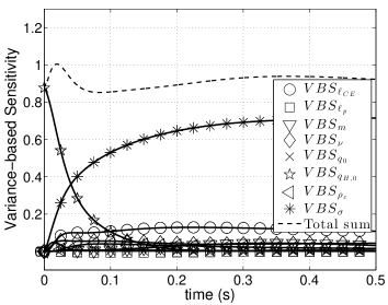
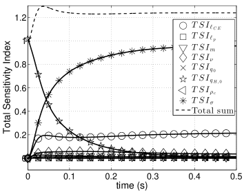
Figure 5: Variance-based sensitivity (left) and total sensitivity index (right) of every parameter of Hatze’s activation dynamics equation

7 Consequences, discussion, conclusions

7.1 A bottom line for comparing Zajac’s and Hatze’s activation dynamics: second order sensitivities

At first sight, Zajac’s activation dynamics [27] is more transparent because it is descriptive in a sense that it captures the physiological behaviour of activity rise and fall in an apparently simple way. It thereto utilises a linear differential equation with well-known properties, allowing for a closed-form solution. It needs only a minimum number of parameters to describe the Ca²⁺-ion influx to the muscle as a response to electrical stimulation: the stimulation $\sigma$ itself as a control parameter, the time constant $\tau$ for an exponential response to a step increase in stimulation, and a third parameter $\beta$ (deactivation boost) biasing both the rise time and saturation value of activity depending on stimulation and activity levels. The smaller $\beta<1$ (deactivation in fact slowed down compared to activation), the faster is the very activity level $q_{Z}\,|_{{}_{\beta=1}}=q_{0}+\sigma\cdot(1-q_{0})$ reached, at which saturation would occur for $\beta=1$. Saturation for $\beta<1$ occurs at a level $q_{Z}=q_{0}+(1-q_{0})/((1-\beta)+\beta/\sigma)$ that is higher than $q_{Z}\,|_{{}_{\beta=1}}$. Altogether, in Zajac’s as compared to Hatze’s activation dynamics, the outcome of setting a control parameter value $\sigma$ in terms of how fast and at which level the activity saturates seems easier to be handled by a controller.

A worse controllability of Hatze’s activation dynamics [8] may be expected from its non-linearity, a higher number of parameters, and their interdendent influence on model dynamics. Additionally, Hatze’s formulation depends on the CE length $\ell_{CErel}$, which makes the mutual coupling of activation with contraction dynamics more interwoven. So, at first sight, this seems to be a more intransparent construct for a controller to deal with a muscle as the biological actuator. Regarding the non-linearity exponent $\nu$, solution sensitivity further depends non-monotonously on activity level, partly even with the strongest influence, partly without any influence. We also found that the solution is more sensitive to its parameters $\sigma$, $\ell_{CErel}$, $\ell_{\rho}$ than is Zajac’s activation dynamics to any of its parameters.

This higher complexity of Hatze’s dynamics becomes even more evident by analysing the second order sensitivities (see (10) as well as (14) for their relative values). They express how a first order sensitivity changes upon variation of any other model parameter. In other words, they are a measure of model entanglement and complexity. Here, we found that the highest values amongst all relative second order sensitivities in Zajac’s activation dynamics are about $-0.8$ ($\tilde{R}_{\beta\,\sigma}$) and $1.6$ ($\tilde{R}_{\beta\,\beta}$). In Hatze’s activation dynamics, the highest relative second order sensitivities are those with respect to $\nu$ or $\ell_{CErel}$ (in particular for $\sigma$, $\rho_{c}$ and $\nu$, $\ell_{CErel}$ themselves) with maximum values between about $-8.0$ ($\tilde{R}_{\ell_{CErel}\,\nu}$, $\tilde{R}_{\nu\,\rho_{c}}$) and $13.4$ ($\tilde{R}_{\ell_{CErel}\,\ell_{CErel}}$, $\tilde{R}_{\ell_{CErel}\,\rho_{c}}$, $\tilde{R}_{\ell_{CErel}\,\sigma}$, $\tilde{R}_{\nu\,\nu}$ at submaximal activity). That is, they are an order of magnitude higher than in Zajac’s activation dynamics.

Yet, we have to acknowledge that Hatze’s activation dynamics contains crucial physiological features that go beyond Zajac’s description.

7.2 A plus for Hatze’s approach: length dependency

It has been established that the length dependency of activation dynamics is both physiological [11] and functionally vital [13] because it largely contributes to low-frequency muscle stiffness. It was also verified that Hatze’s model approach provides a good approximation for experimental data [11]. In that study, $\nu=3$ was used without comparing to the $\nu=2$ case. There seem to be arguments in favour of $\nu=2$ from a mathematical point of view. Especially, the less changeful scaling of the activation dynamics’ characteristics down to very low activity and stimulation levels, and particularly a remaining CE length sensitivity of the dynamics, seem to be an advantage when compared to the $\nu=3$ case. This applies subject to being in accordance with physiological reality. It seems that experimental data with a good resolution of activation dynamics as a response to very low muscular stimulation levels are missing in literature so far: the lowest analysed level in Kistemaker et al. [11] was $\sigma=0.08$, i.e., comparable to the second rows from top in Figs. 2,3.

7.3 An optimal parameter set for Hatze’s activation dynamics plus CE force-length relation

Sensitivity analysis allows to rate Hatze’s approach as an entangled construct. Additionally, Kistemaker et al. [11] decided to choose $\nu=3$ without giving a reason for discarding $\nu=2$. Also, it seemed that they did not perform an algorithmic optimisation on their muscle parameters to fit known shifts in optimal CE length $\Delta\ell_{CE,isom,max}$ at submaximal stimulation levels, i.e., the CE length value where the submaximal isometric force $F_{isom}=F_{isom}(q,\ell_{CE})$ peaks. Accordingly, it seemed worth to perform such an optimisation because $F_{isom}$ generally depends on length $\ell_{CE}$ and activity $q$, and the latter may be additionally biased by an $\ell_{CE}$-dependent capability for building up cross-bridges at a given level $\gamma$ of free Ca²⁺-ions in the sarcoplasma, as formulated in Hatze’s approach: $F_{isom}(q,\ell_{CE})=F_{max}\cdot q(\gamma,\ell_{CE})\cdot F_{\ell}(\ell_{CE})$. Thus, a shift in optimal CE length $\Delta\ell_{CE,isom,max}$ with changing $\gamma$ can occur depending on the specific choices of both the length-dependency of activation $q(\gamma,\ell_{CE})$ (see (3),(4)) and the CE’s force-length relation $F_{\ell}(\ell_{CE})$.

Consequently, we searched for optimal parameter sets of Hatze’s activation dynamics in combination with two different force-length relations $F_{\ell}(\ell_{CE})$: either a parabola [11] or bell-shaped curves [6, 17]. For a given optimal CE length $\ell_{CE,opt}=14.8\,mm$ [22] representing a rat gastrocnemius muscle and three fixed exponent values $\nu=2,3,4$ in Hatze’s activation dynamics (all other parameters as given in section 2), we thus determined Hatze’s constant $\rho_{0}$ and the width parameters of the two different force-length relations $F_{\ell}(\ell_{CE})$ ($WIDTH$ in Kistemaker et al. [11], van Soest and Bobbert [25] and $\Delta W_{asc}=\Delta W_{des}=\Delta W$ in Mörl et al. [17], respectively) by an optimisation approach. The objective function to be minimised was the sum of squared differences between the $\Delta\ell_{CE,isom,max}$ values as predicted by the model and as derived from experiments (see Table 2 in Kistemaker et al. [11]) over five stimulation levels $\sigma=0.55,0.28,0.22,0.17,0.08$. Note that $\gamma=\sigma$ applies in the isometric situation (see (2) and compare (3)).

The optimisation results are summarised in Table 1. The higher the $\nu$ value, the smaller is the optimisation error. Along with that decrease the predicted width values $WIDTH$ or $\Delta W$, respectively. We would, however, tend to exclude the case $\nu=4$ because the predicted width values seem unrealistically low when compared to published values from other sources (e.g., $WIDTH=0.56$ [25], $\Delta W=0.35$ [17]). Furthermore, $\rho_{0}$ decreases with $\nu$ using the parabola model for $F_{\ell}(\ell_{CE})$ whereas it saturates between $\nu=3$ and $\nu=4$ for the bell-shaped model. The bell-shaped model shows the most realistic $\Delta W$ in the case $\nu=3$ ($\Delta W=0.32$). Fitting the same model to other contraction modes of the muscle [17], a value of $\Delta W=0.32$ had been found . In contrast, when using the parabola model, realistic $WIDTH$ values between $0.5$ and $0.6$ are predicted by our optimisation for $\nu=2$. When comparing the optimised parameter values across all start values of the $F_{\ell}(\ell_{CE})$ widths, across all $\nu$ values, and across both $F_{\ell}(\ell_{CE})$ model functions, we find that the resulting optimal parameter sets are more consistent for bell-shaped $F_{\ell}(\ell_{CE})$ than for the parabola function. The bell-shaped force-length relation gives generally a better fit. For each single $\nu$ value, the corresponding optimisation error is smaller when comparing realistic, published $WIDTH$ and $\Delta W$ values that may correspond to each other ($WIDTH=0.56$ [25] and $\Delta W=0.35$ [17]). Additionally, the error values from our optimisations are generally smaller than the corresponding value calculated from Table 2 in Kistemaker et al. [11] ($0.23\,mm$).

In a nutshell, we would say that the most realistic model for the isometric force $F_{isom}$ at submaximal activity levels is the combination of Hatze’s approach for activation dynamics with $\nu=3$ and a bell-shaped curve for the force-length relation $F_{\ell}(\ell_{CE})$ with $\nu_{asc}=3$. As a side effect, we predict that the parameter value $\rho_{0}$, being a weighting factor of the first addend in the compact formulation of Hatze’s activation dynamics (5), should be reduced by about 40% ($\rho_{0}=3.25\cdot 10^{4}\,\frac{l}{mol}$) as compared to the value originally published in Hatze [10] ($\rho_{0}=5.27\cdot 10^{4}\,\frac{l}{mol}$).

7.4 A generalised method for calculating parameter sensitivities

The findings in the last section were initiated by thoroughly comparing two different biomechanical models of muscular activation using a systematic sensitivity analysis as introduced in Gelinas [5] and Lehman and Stark [16], respectively. Starting with the latter formulation, Scovil and Ronsky [21] calculated specific parameter sensitivities for muscular contractions. They applied three variants of this method:

Method 1 applies to state variables that are explicitly known to the modeller as, for example, an eye model [16], a musculo-skeletal model for running that includes a Hill-type muscle model [21], or the activation models analysed in our study. Scovil and Ronsky [21] calculated the change in the value of a state variable averaged over time per a finite change in a parameter value, both normalised to each their unperturbed values. They thus calculated just one (mean) sensitivity value for a finite time interval (e.g., a running cycle) rather than time-continuous sensitivity functions.

Method 2: Whereas Gelinas [5] and Lehman and Stark [16] had introduced the full approach for calculating such sensitivity functions, Scovil and Ronsky [21] distorted this approach by suggesting that the partial derivative of the right hand side of an ODE, i.e., of the rate of change of a state variable, w.r.t. a model parameter would be a “model sensitivity”. The distortion becomes explicitly obvious from our formulation: this partial derivative is just one of two addends that contribute to the rate of change of the sensitivity function (9), rather than it defines the sensitivity of the state variable itself (i.e., the solution of the ODE) w.r.t. a model parameter (8).

Method 3: Scovil and Ronsky [21] had also asked for calculating the influence of, for example, a parameter of the activation dynamics (like the time constant) on an arbitrary joint angle, i.e., a variable that quantifies the overall output of a coupled dynamical system. Of course, the time constant does not explicitly appear in the mechanical differential equation for the acceleration of this very joint angle, which renders applicability of method 2 impossible. The conclusion in Scovil and Ronsky [21] was to apply method 1. Here, the potential of our formulation comes particularly to the fore. It enables to calculate the time-continuous sensitivity of all components of the coupled solution, i.e., any state variable $y_{k}(t)$. This is because all effects of a parameter change are in principle reflected within any single state variable, and the time evolution of a sensitivity according to (9) takes this into account.

In this paper, we have further worked out the sensitivity function approach by Lehman and Stark [16], presenting the differential equations for sensitivity functions in more detail to those modellers who want to apply the method. Furthermore, we enhanced the approach by Lehman and Stark [16] to also calculating the sensitivities of the state variables w.r.t. their initial conditions (12). This should be helpful not only in biomechanics but also, for example, in meteorology when predicting the behaviour of storms [15]. Since initial conditions are often just known approximately but start with the relative sensitivity values of $1$, their influence should be traced to verify how their uncertainty propagates during a simulation. In the case of muscle activation dynamics, the sensitivities $\tilde{S}_{q_{Z,0}}$ and $\tilde{S}_{q_{H,0}}$, respectively, rapidly decreased to zero: initial activity has no effect on the solution early before steady state is reached.

Furthermore, we included a second order sensitivity analysis which is not only helpful for a deeper understanding of the parameter influence but also part of mathematical optimisation techniques [23]. The values of $\tilde{R}_{ijk}$ could be either interpreted as the relative sensitivity of the sensitivity $\tilde{S}_{ik}$ w.r.t. another parameter $\lambda_{j}$ (and vice versa: $\tilde{S}_{jk}$ w.r.t $\lambda_{i}$) or as the curvature of the graph of the solution $y_{k}(t)$ in the $N+M$-dimensional solution-parameter space. The latter may help to connect the results to the field of mathematical optimisation in which the second derivative (Hessian) of a function is often included in objective functions to find optimal parameter sets.

7.5 Deeper understanding through global methods

As a last point for discussion we want to give some additional conclusions arising from the use of a global sensitivity analysis method. In section 6.3 we presented the variance-based sensitivity and the total sensitivity index according to Chan et al. [2]. In the case of Zajac’s activation dynamics, we can strengthen our assumption that there are no significant second and higher order sensitivities with the exception of activation build-up. For an experimenter the only way to get information about the activation time constant $\tau$ is through looking at the first few milliseconds after a change in stimulation, but keeping in mind that the influence is biased by the other parameters.

For Hatze’s activation dynamics, we see that there are higher order sensitivities even in the steady state case. When we talked about controllability of the models we presumed that Zajac’s dynamics would be easier to handle than Hatze’s. But Fig. 5 shows that the stimulation is as well the most important control factor with even a higher importance than in Zajac’s formulation.

Another, at first sight unapparent, result is the importance of $\rho_{c}$. From a strictly differential analysis we concluded that this parameter should have the same sensitivity as $\sigma$ since they both are linear factors in Hatze’s ODE which holds true for their relative sensitivities. The importance, in contrast, is significantly smaller, almost negligible. An explanation can be found if we look at the respective ranges. In the product $\rho_{c}\cdot\sigma\in[4;11]\times[0;1]$ the parameter $\rho_{c}$ has a wider range but only serves as a lever for $\sigma$ which has a much larger percentage changeability. The same observation can be made for the parameter $\nu$ which has a very small variability throughout literature. Although the differential sensitivity is quite large, $\nu$ has not much importance for the model output.

Nevertheless the advantages of a global sensitivity analysis the findings must be treated with caution because we have a whole dynamical system summed up to a single function per parameter. In sections 6.1 and 6.2 we evaluated the local sensitivity of Zajac’s and Hatze’s formulation each at 8 different points in the parameter space. Therefore we saw the effects of each parameter on the solution in some borderline cases which are averaged in a global analysis.

Summarizing the findings of this article it takes three components to a meaningful sensitivity analysis: a deep understanding of the model, a complete mathematical investigation and an interpretation of the results based on the model itself.

Table 1: Parameters minimising the sum over five submaximal stimulation levels $\gamma=\sigma=0.55,0.28,0.22,0.17,0.08$ of squared differences between shifts in optimal CE length $\Delta\ell_{CE,isom,max}(\gamma)$ ($\Delta l_{MA,opt}$ by Roszek et al. (1994) in third column of Table 2 in Kistemaker et al. [11]) at these levels predicted by the model with the isometric force $F_{isom}(q,\ell_{CE})=F_{max}\cdot q(\gamma=\sigma,\ell_{CE})\cdot F_{\ell}(\ell_{CE})$ and by experiments; simulated data represent a rat gastrocnemius muscle with an optimal CE length $\ell_{CE,opt}=14.8\,mm$ [22]; start value of $\rho_{0}$ was $6.0\cdot 10^{4}\frac{l}{mol}$; the exponents of the bell-shaped force-length relations $F_{\ell}(\ell_{CE})$ were fixed according to Mörl et al. [17] ($\nu_{asc}=3$, $\nu_{des}=1.5$), the corresponding width values in the ascending and descending branch were assumed to be equal: $\Delta W_{asc}=\Delta W_{des}=\Delta W$; van Soest and Bobbert [25] and Kistemaker et al. [11] used a parabola for $F_{\ell}(\ell_{CE})$; for all other model parameters see sections 7.3 and 2; optimisation was done by $fminsearch$ (Nelder-Mead algorithm) in MATLAB with error tolerances of $10^{-8}$; $error$ is the square-root of the above mentioned sum divided by five; corresponding error value given in Table 2 in Kistemaker et al. [11] was $0.23\,mm$.

$\nu$	bell-shaped [6, 17]			parabola [25, 11]
	$\Delta W_{start}=0.25$			$WIDTH_{start}=0.46$
	$\Delta W\,[]$	$\rho_{0}\,[10^{4}\frac{l}{mol}]$	$error\,[mm]$	$WIDTH\,[]$	$\rho_{0}\,[10^{4}\frac{l}{mol}]$	$error\,[mm]$
2	0.46	3.80	0.08	0.63	8.78	0.10
3	0.32	3.25	0.05	0.41	5.45	0.07
4	0.26	3.20	0.02	0.34	4.60	0.05
	$\Delta W_{start}=0.35$			$WIDTH_{start}=0.56$
	$\Delta W\,[]$	$\rho_{0}\,[10^{4}\frac{l}{mol}]$	$error\,[mm]$	$WIDTH\,[]$	$\rho_{0}\,[10^{4}\frac{l}{mol}]$	$error\,[mm]$
2	0.45	3.80	0.07	0.53	6.92	0.11
3	0.32	3.30	0.05	0.41	5.67	0.07
4	0.26	3.20	0.02	0.34	4.55	0.05
	$\Delta W_{start}=0.45$			$WIDTH_{start}=0.66$
	$\Delta W\,[]$	$\rho_{0}\,[10^{4}\frac{l}{mol}]$	$error\,[mm]$	$WIDTH\,[]$	$\rho_{0}\,[10^{4}\frac{l}{mol}]$	$error\,[mm]$
2	0.45	3.78	0.07	0.55	7.35	0.11
3	0.32	3.25	0.05	0.41	5.35	0.07
4	0.26	3.20	0.02	0.34	4.56	0.05

References

- Benker [2005] Benker, H., 2005. Differentialgleichungen mit MathCad und MatLab. Vol. 1. Springer.
- Chan et al. [1997] Chan, K., Saltelli, A., Tarantola, S., 1997. Sensitivity analysis of model output: variance-based methods make the difference. In: Andradóttir, S., Healy, K., Withers, D., Nelson, B. (Eds.), Proceedings of the 29th Conference on Winter Simulation. Winter Simulation Conference. IEEE Computer Society, Washington, DC, USA, pp. 261–268.
- Cole et al. [1996] Cole, G., van den Bogert, A., Herzog, W., Gerritsen, K., 1996. Modelling of force production in skeletal muscle undergoing stretch. J. Biomechanics 29, 1091 – 1104.
- Frey [2003] Frey, H. C. ; Mokthari, A. . D. T., 2003. Evaluation of selected sensitivity analysis methods based upon application to two food safety process risk models. Tech. rep., Computational Laboratory for Energy, North Carolina State University.
- Gelinas [1976] Gelinas, R. D. R., 1976. Sensitivity analysis of ordinary differential equation systems - a direct method. Journal of Computational Physics 21, 123–143.
- Günther et al. [2007] Günther, M., Schmitt, S., Wank, V., 2007. High-frequency oscillations as a consequence of neglected serial damping in Hill-type muscle models. Biological Cybernetics (97), 63–79.
- Haeufle et al. [2014] Haeufle, D., Günther, M., Bayer, A., Schmitt, S., 2014. Hill-type muscle model with serial damping and eccentric force-velocity relation. Journal of Biomechanics, published online.
- Hatze [1977] Hatze, H., 1977. A myocybernetic control model of skeletal muscle. Biological Cybernetics 25, 103–119.
- Hatze [1978] Hatze, H., 1978. A general myocybernetic control model of skeletal muscle. Biological Cybernetics 28, 143–157.
- Hatze [1981] Hatze, H., 1981. Myocybernetic control models of skeletal muscle. University of South Africa.
- Kistemaker et al. [2005] Kistemaker, D., van Soest, A., Bobbert, M., 2005. Length-dependent [Ca2+] sensitivity adds stiffness to muscle. Journal of Biomechanics 38 (9), 1816–1821.
- Kistemaker et al. [2006] Kistemaker, D., van Soest, A., Bobbert, M., 2006. Is equilibrium point control feasible for fast goal-directed single-joint movements? Journal of Neurophysiology 95 (5), 2898–2912.
- Kistemaker et al. [2007] Kistemaker, D., van Soest, A., Bobbert, M., 2007. A model of open-loop control of equilibrium position and stiffness of the human elbow joint. Biological Cybernetics 96 (3), 341–350.
- Kolda [2006] Kolda, B. W. B. T. G., 2006. Algorithm 862: Matlab tensor classes for fast algorithm prototyping. ACM Transactions on Mathematical Software 32 (4), 635–653.
- Langland [2002] Langland, R., 2002. Initial condition sensitivity and error growth in forecasts of the 25 january 2000 east coast snowstorm. AMS 130 (4), 957–974.
- Lehman and Stark [1982] Lehman, S., Stark, L., 1982. Three algorithms for interpreting models consisting of ordinary differential equations: sensitivity coefficients, sensitivity functions, global optimization. Mathematical Biosciences 62 (1), 107–122.
- Mörl et al. [2012] Mörl, F., Siebert, T., Schmitt, S., Blickhan, R., Günther, M., 2012. Electro-mechanical delay in Hill-type muscle models. Journal of Mechanics in Medicine and Biology 12 (5), 85–102.
- Saltelli and Annoni [2010] Saltelli, A., Annoni, P., 2010. How to avoid a perfunctory sensitivity analysis. Environmental Modelling & Software 25 (12), 1508–1517.
- Saltelli [2000] Saltelli, A. ; Chan, K. . S. E., 2000. Sensitivity Analysis, 1st Edition. John Wiley.
- Scherzer [2009] Scherzer, O., 2009. Mathematische Modellierung - Vorlesungsskript. Universität Wien.
- Scovil and Ronsky [2006] Scovil, C., Ronsky, J., 2006. Sensitivity of a Hill-based muscle model to pertubations in model parameters. J. Biomechanics 39, 2055–2063.
- Siebert et al. [2014] Siebert, T., Till, O., Blickhan, R., 2014. Work partitioning of transversally loaded muscle: experimentation and simulation. Computer Methods in Biomechanics and Biomedical Engineering 17 (3), 217–229.
- Sunar and Belegundu [1991] Sunar, M., Belegundu, A., 1991. Trust region methods for structural optimization using exact second order trust region method for structural optimization using exact second order sensitivity. International Journal for Numerical Methods in Engineering 32, 275–293.
- van Soest [1992] van Soest, A., 1992. Jumping from structure to control: a simulation study of explosive movements. Ph.D. thesis, Vrije Universiteit, Amsterdam.
- van Soest and Bobbert [1993] van Soest, A., Bobbert, M., 1993. The contribution of muscle properties in the control of explosive movements. Biological Cybernetics 69 (3), 195–204.
- Vukobratovic [1962] Vukobratovic, R. T. M., 1962. General Sensitivity Theory. American Elsevier, New York.
- Zajac [1989] Zajac, F. E., 1989. Muscle and tendon: Properties, models, scaling, and application to biomechanics and motor control. Crit. Rev. Biomed. Eng 17 (4), 359–411.
- ZivariPiran [2009] ZivariPiran, H., 2009. Efficient simulation, accurate sensitivity analysis and reliable parameter estimation for delay differential equations. Ph.D. thesis, University Toronto.