Understanding Common Perceptions from Online Social Media

Abstract

Modern society habitually uses online social media services to publicly share observations, thoughts, opinions, and beliefs at any time and from any location. These geo-tagged social media posts may provide aggregate insights into people’s perceptions on a broad range of topics across a given geographical area beyond what is currently possible through services such as Yelp and Foursquare. This paper develops probabilistic language models to investigate whether collective, topic-based perceptions within a geographical area can be extracted from the content of geo-tagged Twitter posts. The capability of the methodology is illustrated using tweets from three areas of different sizes. An application of the approach to support power grid restoration following a storm is presented.

1 Introduction and Motivation

Online social media services are now deeply rooted in our modern culture and people routinely turn to these services to share their thoughts and opinions. These frequent updates can provide tremendous insights into how people perceive the world around them. A significant portion of these updates are shared via smartphones and mobile devices, and hence, have location information embedded in them. This geo-tagging offers a unique opportunity to understand how the content or what of the posts is influenced by the location or from where the posts are shared [4]. Such linking of “what” to “where” can be used to support many geographic information retrieval systems [1]. Commercial agencies can also use this association between perception and location to tailor their marketing strategies to geographic demands [10].

Presently, geo-tagged social media posts are linked to specific businesses using services such as Yelp and Foursquare. Through this linking, people can share their reviews and experiences and alert friends to their whereabouts. Opinions about specific businesses, however, may not offer insights into how people feel about the underlying abstract notions or topics. For example, reviews about specific fast food restaurants cannot indicate whether people in the area like to eat fast food, or that eating fast food is popular. Instead, posts that talk about fast food generally, with or without reference to specific restaurants, provide clues about area-wide perceptions on the topic of fast food.

This paper proposes a methodology that uses social media posts to identify localities where a specific topic-based perception runs strong. Partitioning a geographic area into non-overlapping sub-areas, the methodology trains probabilistic language models over posts from these sub-areas. This ensemble of models is then queried with a phrase defining a topic-based perception to identify sub-areas where that perception runs strong. Illustrations using Twitter feeds from three areas of vastly different sizes, population densities, and other characteristics show that despite the diversity, the methodology can identify sub-areas with strong perceptions for several common topics. The paper concludes with an industrial application of the methodology to support efficient power recovery following a major weather storm.

The paper is organized as follows: Section 2 presents our methodology. Section 3 describes Twitter data. Section 4 illustrates the methodology. Section 5 applies it to storm damage response. Section 6 compares related work. Conclusions and future directions are in Section 7.

2 Locating Perceptions

In this section, we motivate and present the methodology for finding perceptions.

2.1 Defining Perceptions

People’s perceptions about various topics may be embodied in their spoken language and now in their social media posts. These topic-based perceptions may be influenced by the general characteristics of an area and also by specific local features. For example, although people across New York City may frequently talk and post about traffic congestion and delays, this issue is unlikely to be on their minds as they stroll through Central Park. Because it is impossible to exhaustively define all topics and their perceptions, we propose a flexible approach which models the language of the social media posts for each sub-area within a given area. These language models can then be queried with multi-word phrases which define a perception about a given topic to identify sub-areas which strongly represent that topic-based perception. For example, to identify perceptions of stressful (slow) traffic, we can use the query ”hate traffic” (”traffic is slow”). Note that sub-areas with stressful traffic may or may not overlap those with slow traffic.

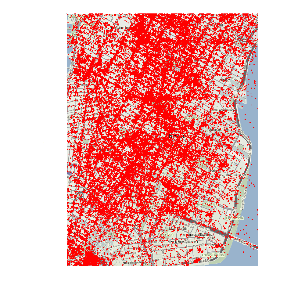
(a) NYC: Local-level

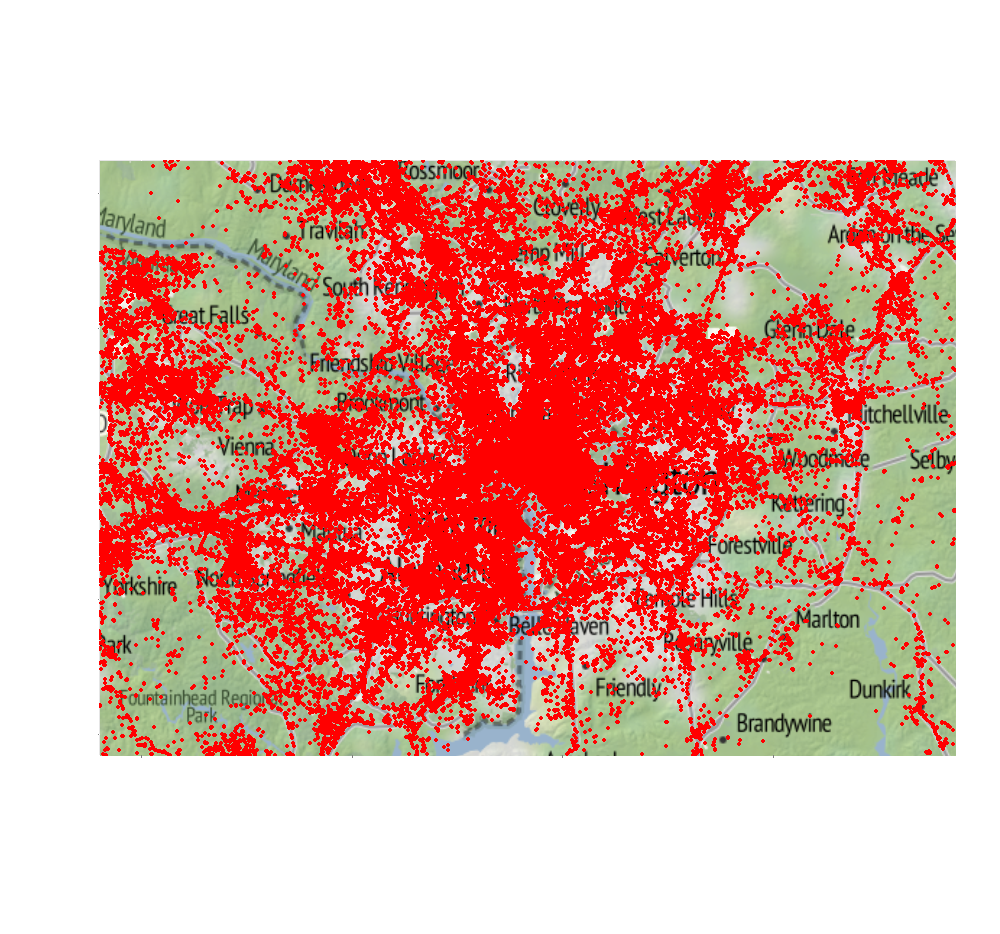
(b) DC: District-level

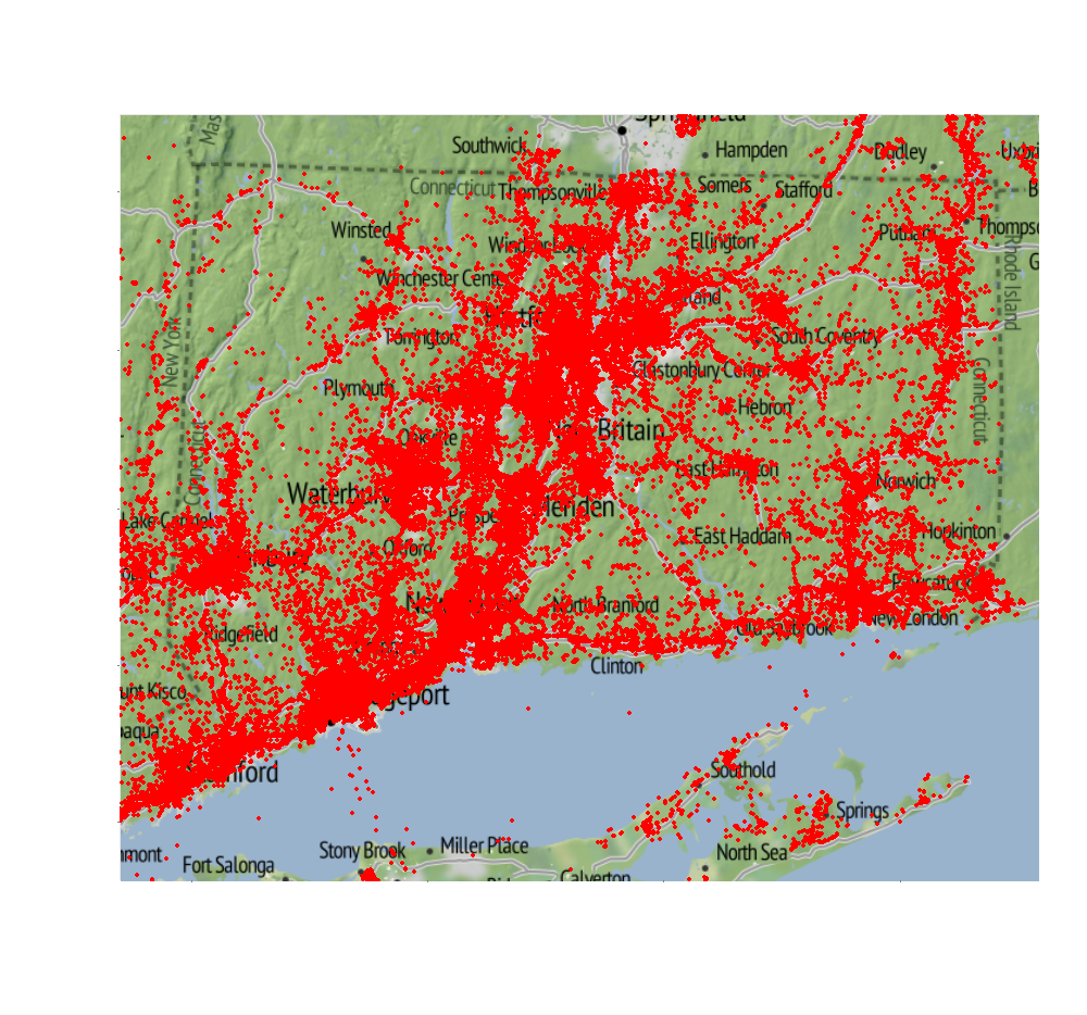
(c) CT: Region-level

Figure 1: Tweet Distribution in the Areas

2.2 Specifying Language Models

A language model captures the features of the written language in a collection of documents or a training corpus. It defines a probability distribution over all $n$-grams, where an $n$-gram is an ordered sequence of $n$ words $(w_{1},....,w_{n})$. We define language models for non-overlapping sub-areas $\ell_{i}$ which comprise an area $\mathcal{L}$. The maximum likelihood estimate of an $n$-gram, computed over a corpus of social media posts within $\ell_{i}\in\mathcal{L}$, is given by [3]:

$$P_{\ell_{i}}(w_{1},....w_{n})=\frac{c(w_{1},...w_{n})}{c(w_{1},...,w_{n-1})}$$

where $c(.)$ is the number of times the sequence appears in the posts. The probability that the language within a sub-area generates a phrase $T=(w_{1},...,w_{k})$ is computed as the product of the probabilities of the $n$-grams that comprise $T$:

$$P(T|\ell_{i})=\prod_{j=n}^{k}P_{\ell}(w_{j-n+1},...,w_{j})$$

Contextual information increases with $n$ as higher order sequences of words are considered. However, because the frequency that larger sequences appear in social media posts is very low, prevalent language models over these posts restrict to the lowest order unigrams ($1$-grams), which model distinct words independent of their order [16, 5, 11]. Unigrams cannot model perceptions because these must be understood in the context of some topic or subject. For example, unigrams trained over “I love driving” and “I hate driving” will model the perceptions of “love” and “hate” but will not associate them with the topic of “driving”. Bigrams, on the other hand, can model the perceptions “I love”, “love driving”, “I hate”, and “hate driving” and associate them with a person (“I”) and the act of driving. Thus, unigrams can only recognize “love” or “hate”, while bigrams actually identify what is being loved or hated. However, because social media posts may contain numerous distinct bigrams presenting unique thoughts on various topics, the estimates of bigrams over these posts may be inaccurate. To improve this accuracy, we model the probability of bigram estimates using a linear interpolation of both the bigram and unigram estimates. This interpolation compensates for the low count of a bigram (e.g. “love driving”) by incorporating the expected higher count of the unigram “driving”. Thus, for a sub-area $\ell_{i}$, the probability of observing the bigram $(w_{j-1},w_{j})$ is given as:

$$P_{\ell_{i}}(w_{j-1},w_{j})=\lambda_{1}c(w_{j-1},w_{j})/c(w_{j-1})+\lambda_{2}c(w_{j})/|W(\ell_{i})|$$

where $\lambda_{1}+\lambda_{2}=1$, $|W(\ell_{i})|$ is the number of distinct words in all posts in $\ell_{i}$ and $c(w_{j})/|W(\ell_{i})|$ is the estimate of the unigram that completes the bigram [3].

We use smoothing to compensate for the probability of future unseen bigrams, which allocates some of the probability of the training bigrams to those that are as yet unobserved [6]. The Modified Kneser-Ney (MKN) smoothing algorithm [9] is chosen because of its superior performance with interpolated language models [6]. The MKN algorithm subtracts a constant $\hat{d}$ from the observed frequency of every known bigram. It then estimates the likelihood that an unknown bigram $(w_{j-1},w_{j})$ will appear using a modified estimate of the unigram $w_{j}$, where only the number of distinct bigrams that $w_{j}$ completes is considered:

$$P_{c}(w_{j})=\frac{|\{w:c(w,w_{j})>0\}|}{\sum_{v}|\{w:c(w,v)>0\}|}$$

and then weighing this proportion by the probability mass $\lambda(w_{j-1})$ taken from the known bigrams:

$$\lambda(w_{j-1})=\frac{\hat{d}|\{w:c(w_{j-1},w)>0\}|}{c(w_{j-1})}$$

Thus, under MKN smoothing the probability of observing a bigram becomes:

$$P_{\ell}(w_{j-1},w_{j})=\frac{\max(c(w_{j-1},w_{j})-\hat{d},0)}{c(w_{j-1})}+\lambda(w_{j-1})P_{c}(w_{j})$$

If $(w_{j-1},w_{j})$ is unknown, the probability is just given by $\lambda(w_{j-1})P_{c}(w_{j})$, and if it is known, the probability is given as a linear interpolation of the modified bigram and unigram estimates. Note that the modified unigram estimate $P_{c}(w_{j})$ is superior to $c(w_{j})/|W(\ell)|$ because under $P_{c}(w_{j})$ words that appear frequently but within few distinct contexts will not strongly influence the probability of the bigram. We estimate $\hat{d}$ such that the log-likelihood that the model generates a given bigram is maximized:

$$\hat{d}=\arg\max_{d}\sum_{v}c(v,w_{j})\log P_{\ell}(v,w_{j})$$

This has a closed form approximation depending on whether $c(w_{i-1},w_{i})$ is equal to $1$, $2$, or $\geq 3$ [14]. Using these approximations, we set $\hat{d}$ equal to $d_{1},d_{2}$, or $d_{3}$ respectively:

$$d_{1}=1-\frac{2n_{2}n_{1}}{n_{1}(n_{1}+2n_{2})}$$

$$d_{2}=2-\frac{3n_{3}n_{1}}{n_{2}(n_{1}+2n_{2})}$$

$$d_{3}=3-\frac{4n_{4}n_{1}}{n_{3}(n_{1}+2n_{2})}$$

with $n_{i}$ is the number of bigrams with frequency $i$.

The ensemble of language models, one for each sub-area, is then queried to compute the probability that a phrase $T$ is generated from a sub-area $\ell_{i}$ using Bayes rule:

$$P(\ell_{i}|T)=\frac{P(T|\ell_{i})P(\ell_{i})}{\sum_{j}P(T|\ell_{j})P(\ell_{j})}$$

$P(\ell_{i})$ is the prior probability that a social media post is from sub-area $\ell_{i}$ and is given by $N(\ell_{i})/N(\mathcal{L})$. $N(\ell_{i})$ is the number of posts in $\ell_{i}$ and $N(\mathcal{L})$ is the total number of posts in the entire area $\mathcal{L}$. Finally, we we define define $P(T|\ell_{i})$ as:

$$P(T|\ell_{i})=\prod_{j=2}^{k}P_{\ell_{i}}(w_{j-1},w_{j})$$

3 Data Description

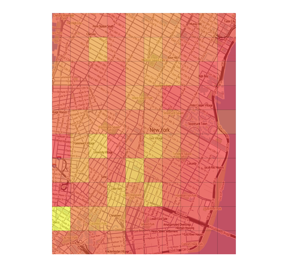
(a) “Restaurant”

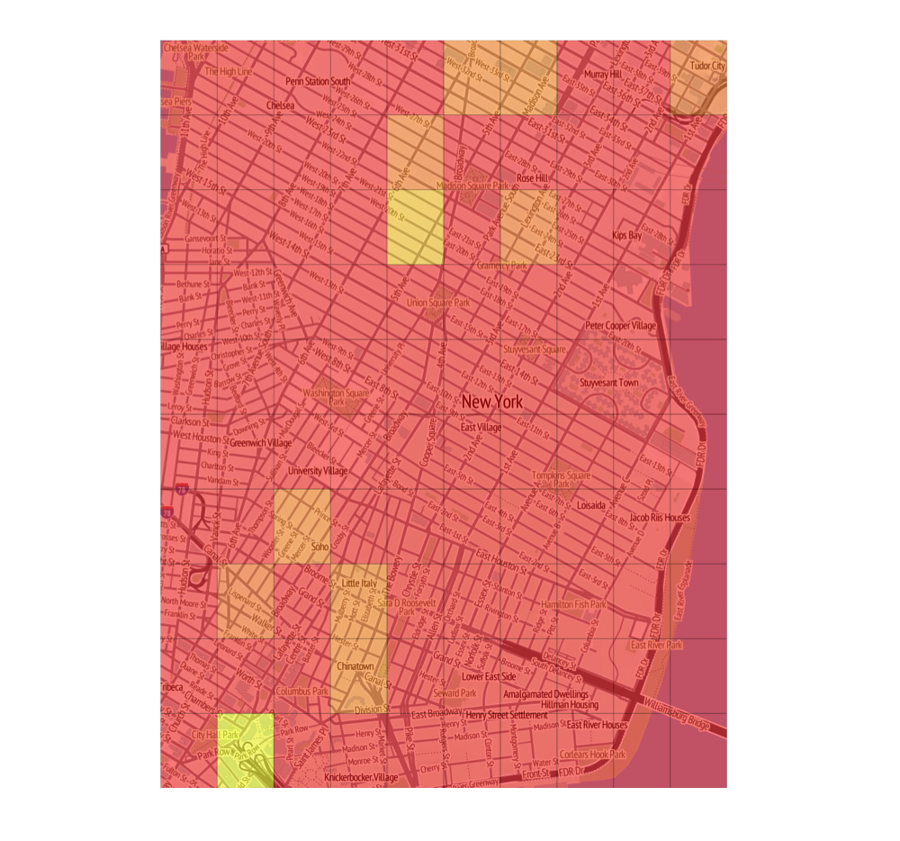
(b) “Italian restaurant”

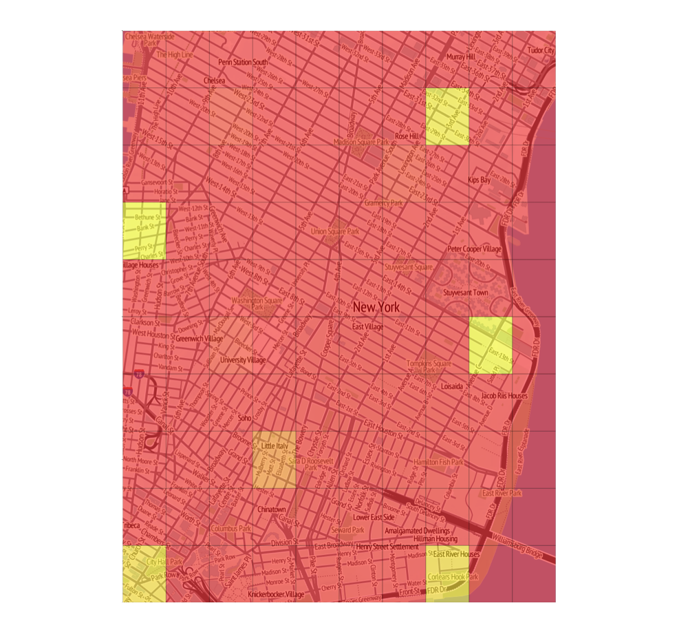
(c) “Went to a great Italian restaurant”

Figure 2: Local-level Perceptions in NYC

We harvested geo-tagged tweets from Twitter between January $29^{th}$ and February $28^{th}$ 2013 from three areas, namely, Downtown Manhattan in New York City (NYC), the greater Washington D.C. area and its surroundings (DC), and the entire state of Connecticut (CT). Although these areas can be partitioned according to town and city jurisdictions or even by zip code, for the sake of illustration, we divide them into $100$ equal sub-areas along a $10\times 10$ grid using latitudinal and longitudinal coordinates. The partitions of each area differ widely: (i) NYC sub-areas include a few blocks and provide a local-level perspective; (ii) DC sub-areas include substantial portions of cities, suburbs, and interstates providing a district-level perspective; and (iii) CT sub-areas contain multiple towns, entire cities and woods offering a region-level perspective.

For each area, we eliminated non-English tweets and those without geo-tags. Table 1 shows that the tweet density in NYC is an order higher than DC and two orders higher than CT. The lower densities in DC and CT, however, do not impede training of the language models, because in each area tweet distributions conform to population spread as shown in Figure 1 [7]. Thus, tweets in NYC are almost uniform, in DC they cluster around major cities and follow paths to major highways, and in CT they concentrate around the three major interstates, with sparse densities in the woods and farmland towns.

(a) “traffic”

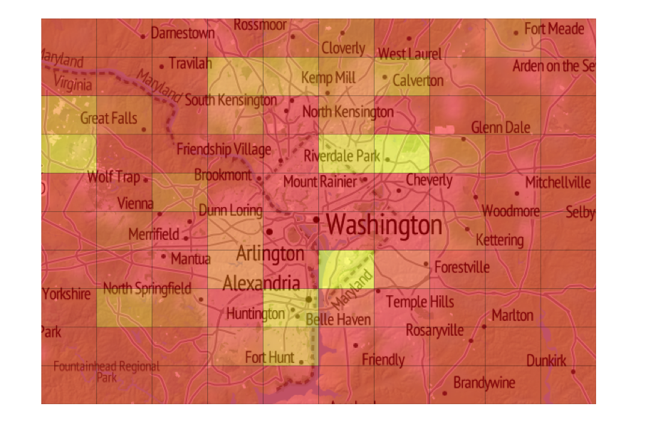
(b) “traffic during commute”

Figure 3: District-level Perceptions in DC

Area	Sub-area	Area Size	Tweets	Density
NYC	Local	82.3km2	110,924	1,347/km2
DC	District	3,452km2	394,072	114/km2
CT	County	22,140km2	355,678	16/km2

Table 1: Area-wise Summary of Tweets

Geo-tagged tweets were further pre-processed by converting all words to lowercase and by stripping punctuation, hashtags (terms starting with #), username replies (terms beginning with $@$), and Web links. Common words such as “at”, “the”, and “or” lack contextual information, and hence, were eliminated using a stopword list of $200$ most frequently used words. The stopword list was limited to $200$ which is approximately equal to $1\%$ of the average number of distinct words across each area. We also include a “catch all” unigram “$<$misc$>$” to aggregate the probability of all words that occur only once. It also accounts for miscellaneous, shorthand, mis-spelled, and other user-specific notations. On an average $3.16\%$ of the words in each area were mapped to “$<$misc$>$”, suggesting that we can control this source of distortion without impacting the models’ fidelity.

4 Illustrations

In this section, we illustrate how our approach can identify sub-areas with strong topic-based perceptions.

4.1 Perceptions in NYC

Downtown Manhattan is a popular tourist destination and includes Chinatown and Little Italy as well as Broadway and Penn Station. Given its multi-cultural neighborhoods and popularity, this area is rife with many types of eateries, due to which we extract perceptions about restaurants. Figure 2a displays the results in the form of a heat map, produced by a generic query “restaurants”. Brighter shades across many sub-areas indicate that people discuss restaurants broadly. Figure 2b shows the results of a refined query “Italian restaurants”. The heat map now concentrates on fewer sub-areas, mostly in the southwest, which corresponds to Little Italy. It also includes northern sub-areas; home to many high-end Italian restaurants. Finally, a specific query “went to a great Italian restaurant” produces Figure 2c which tells us that this perception is most strongly present in Little Italy, and at the entrances to the Holland Tunnel, Brooklyn and Williamsburg Bridges. That this perception is strong in sub-areas used to leave the city suggests that visitors may be more inclined to share their satisfaction about a great meal in Little Italy compared to the city’s residents.

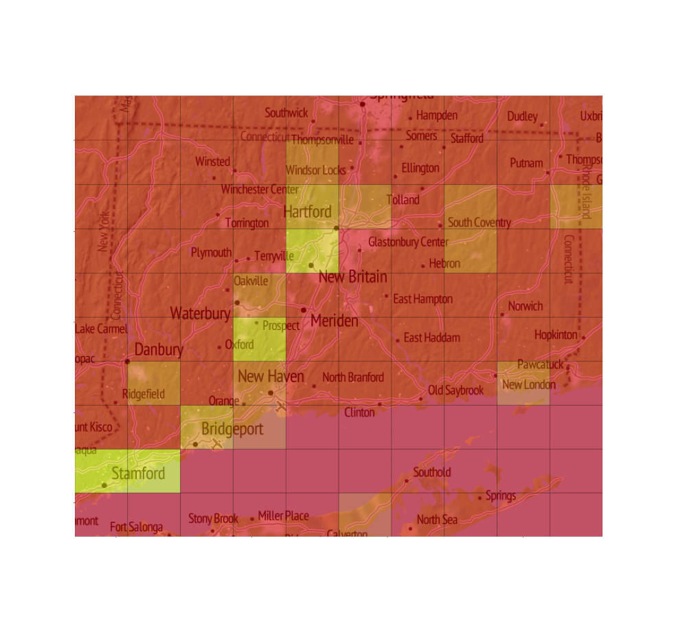
(a) “crime”

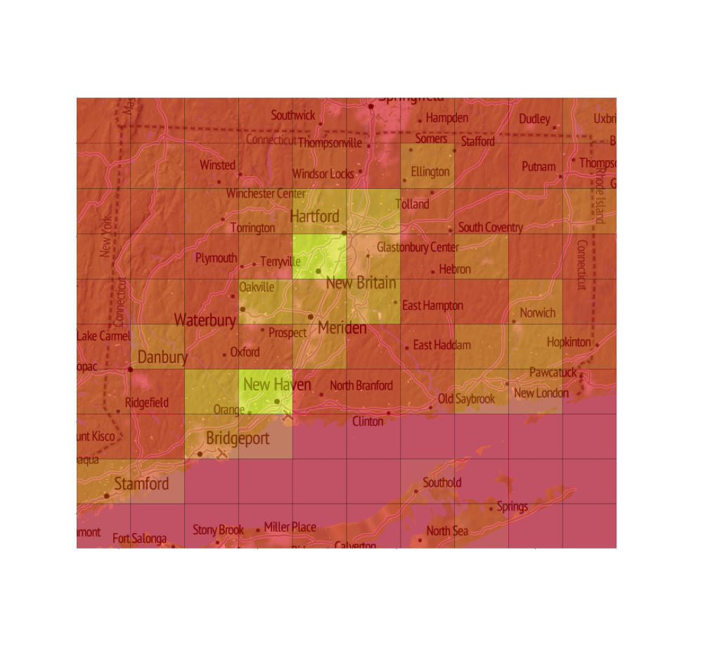
(b) “hospital”

Figure 4: Region-level Perceptions in CT

4.2 Perceptions in DC

This area encompasses Washington D.C. and the surrounding suburbs. Here, sub-areas include entire communities, parts of Washington D.C., portions of the I-95/495 interstate loop infamous for its heavy traffic, regional parks, and major roads that connect Washington D.C. to Maryland and Virginia. The city is dominated by office parks, federal agencies, and corporate headquarters bringing in a large number of commuters from outside towns and suburbs. We thus extract perceptions on “traffic” for this area. The heat map in Figure 3a, resulting from a generic query “traffic”, shows that traffic is most strongly perceived inside and around the four sub-areas of downtown and decreases in prominence as we go farther away. The heat map in Figure 3b, resulting from a more nuanced query “traffic during commute”, finds that people do not discuss traffic and commute within the city, but as expected in the sub-areas which contain portions of the I-95/495 interstate loop and those to the west neighboring Dulles Airport.

4.3 Perceptions in CT

This area covers the state of Connecticut featuring large sub-areas that include entire towns and cities. A hot-button issue that many people consider when deciding to relocate to a neighborhood is the public perception of crime. City and town governments must thus be aware of how crime is perceived in their jurisdictions. The heat map in Figure 4a, resulting from a generic query “crime”, suggests that the people of CT do not think about crime except for sub-areas along the I-91 interstate containing the cities of New Haven, Bridgeport, Stamford, and Hartford, which are notorious for its dangerousness. Because a state encompasses a large area, we also extract perceptions about topics that are less likely to be thought of at a local- and district-level. The heap map in Figure 4b, resulting from the query “hospital”, shows that the hottest sub-areas coincide with the Yale-New Haven Hospital and UConn Health Center. Also, adjacent sub-areas are more likely to think of hospitals, compared to other sub-areas in the state.

5 Storm Power Grid Damage Response

The above examples illustrate the capability of our approach to identify varied topic-based perceptions. We now discuss how such identification can be leveraged for a disaster response scenario. Natural and other disasters can create potentially life-threatening conditions because of their destructive impact on an electric power grid. Responding to such outages efficiently and quickly can minimize this damage and reduce the costs of restoration and loss of productivity. Currently, utilities rely on experts to estimate locations of outages and the type and extent of damages in order to dispatch appropriate crews and materials. We describe how public perceptions on the damages caused to the power grid following a storm provides situational or “on-the-ground” data supporting the expert’s analysis. On January 31^st 2013, the CT area experienced hurricane force winds causing widespread power outages. The heat map in Figure 5, resulting from the query “power outage”, shows that locations of this perception correspond to the power outage map . Zooming into an area northeast of Hartford, generates another heat map for the same perception, which now highlights a residential block. Zooming in even further identifies specific places on the streets, which may correspond to houses or electric poles. Based on this data, experts can tag these streets as prone to power loss. They can analyze the power grid in the area to determine what components failed, and using tweets within the highlighted sub-areas, hypothesize about the source of damage (e.g. downed trees crushing overhead lines). The appropriate crews and components can then be dispatched to quickly repair these failures.

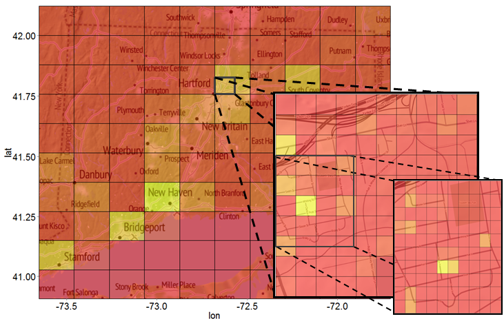
Figure 5: Perception of “power outage” in CT

6 Related Research

Language models have been built over social media posts for a variety of purposes. Iskandar et al. develop a query likelihood model with Dirichlet smoothing to retrieve content from social media and Wikipedia articles [2]. Li predicts the point-of-interest of a tweet with a unigram language model [11]. The models are also combined with location information to evaluate the origin of tweets. Kinsella et al. estimate cities from which tweets originate by comparing KL-divergences among language models [8]. Chandra et al. also predict originating cities based on unigram models over tweet-reply chains [5]. Chang predicts positions based on the spatial usage of words in the tweets [15], Sadilek et al. incorporate the position of friends and content of tweets for prediction [13], Liu et al consider check-in histories with tweet content [12] and Wing et al use unigram models of tweet content across areas within geo-grids [16].

This work differs from contemporary efforts because rather than focusing on a specific set of tasks, we develop language models to generally identify perceptions of users across geographic areas. Also, our sophisticated language model uses smoothing to combine accurate estimation of unigrams with contextual information in bigrams compared to the prevalent models that consider only unigrams.

7 Conclusions and Future Work

This paper presented a methodology to identify where perceptions about a topic are strongly represented across a given geographic area. Central to the methodology are language models that can be queried using phrases that define any kind of perception for any topic. Without any a priori information and aid of external data sources, we demonstrate how the approach can identify where a specific topic-based perception is strongly represented in sub-areas with sizes ranging from just a few urban blocks to entire cities.

In the future, we plan to enhance the methodology with geographic and temporal variations in word usage. We will also explore the use of the methodology for many different applications including location prediction, storm and disaster management, and analytics for city planning and public services including mass transit.

References

- [1] G. Andogah. Geographically Constrained Information Retrieval. PhD thesis, University of Groningen, 2010.
- [2] D. Awang Iskandar, J. Pehcevski, J. Thom, and S. Tahaghoghi. Social media retrieval using image features and structured text. In Proc. of Workshop on Initiative for the Evaluation of XML Retrieval, pages 358–372, 2007.
- [3] L. R. Bahl, F. Jelinek, and R. L. Mercer. A maximum likelihood approach to continuous speech recognition. IEEE Transactions on Pattern Analysis and Machine Intelligence, pages 179–190, 1983.
- [4] R. B. Brandom. Between Saying and Doing: Towards an Analytic Pragmatism: Towards an Analytic Pragmatism. OUP Oxford, 2008.
- [5] S. Chandra, L. Khan, and F. Muhaya. Estimating twitter user location using social interactions–a content based approach. In Intl. Conf. on Social Computing, pages 838–843. IEEE, 2011.
- [6] S. Chen and J. Goodman. An empirical study of smoothing techniques for language modeling. In Proc. of Association for Computational Linguistics Annual Meeting, pages 310–318. Association for Computational Linguistics, 1996.
- [7] P. Division. Land Area, Population, and Density for Plances and (in selected states) County Subdivisions: 2000. United States Census Bureau, 2000.
- [8] S. Kinsella, V. Murdock, and N. O’Hare. I’m eating a sandwich in Glasgow: modeling locations with tweets. In Proceedings of Intl. Workshop on Search and Mining User-Generated Content, pages 61–68. ACM, 2011.
- [9] R. Kneser and H. Ney. Improved backing-off for m-gram language modeling. In Intl. Conference on Acoustics, Speech, and Signal Processing, volume 1, pages 181–184. IEEE, 1995.
- [10] J. A. Lesser and M. A. Hughes. The generalizability of psychographic market segments across geographic locations. Journal of Marketing, pages 18–27, 1986.
- [11] W. Li, P. Serdyukov, A. P. de Vries, C. Eickhoff, and M. Larson. The Where in the Tweet. In Proc. of Intl. Conference on Knowledge Management, 2011.
- [12] H. Liu, B. Luo, and D. Lee. Location Type Classification Using Tweet Content. In Proc. of Intl Conference on Machine Learning and Applications, 2012.
- [13] A. Sadilek, H. Kautz, and J. Bigham. Finding Your Friends and Following Them to Where You Are. In Proc. of Intl. Coference on Web Search and Data Mining, 2012.
- [14] M. Sundermeyer, R. Schlüter, and H. Ney. On the estimation of discount parameters for language model smoothing. Interspeech, 2011.
- [15] H. wen Change, D. Lee, M. Eltaher, and J. Lee. @Phillies Tweeting from Philly? Predicting Twitter User Locations with Spatial Word Usage. In Proc. of Intl. Conference on Advances in Social Networks Analysis and Mining, pages 111–118. IEEE, 2012.
- [16] B. Wing and J. Baldridge. Simple supervised document geolocation with geodesic grids. In Proc. of the Annual Meeting of the Association for Computational Linguistics, volume 1, pages 955–964, 2011.