Bounds for the genus of a normal surface

Abstract

This paper gives sharp linear bounds on the genus of a normal surface in a triangulated compact, orientable 3–manifold in terms of the quadrilaterals in its cell decomposition—different bounds arise from varying hypotheses on the surface or triangulation. Two applications of these bounds are given. First, the minimal triangulations of the product of a closed surface and the closed interval are determined. Second, an alternative approach of the realisation problem using normal surface theory is shown to be less powerful than its dual method using subcomplexes of polytopes.

57N10; 57Q15; 57M20; 57N35; 53A05

1 Introduction

The theory of normal surfaces, introduced by Kneser [31] and further developed by Haken [20, 21], plays a crucial role in $3$–manifold topology. Normal surfaces allow topological problems to be translated into algebraic problems or linear programs, and they are the key to many important advances over the last $50$ years, including the solution of the unknot recognition problem by Haken [20], the $3$–sphere recognition problem by Rubinstein and Thompson [39, 40, 44], and the homeomorphism problem for Haken 3–manifolds by Haken, Hemion and Matveev [21, 23, 36].

A normal surface in a triangulated 3–manifold is decomposed into triangles and quadrilaterals. It is well known that the topology of a normal surface is determined by the quadrilaterals in its cell structure. In this paper, we give a sharp linear bound on the genus $g$ of a closed, orientable normal surface in terms of the number $q$ of quadrilateral discs in the surface; namely $3q\geq 2g.$ This bound is sharp and significantly improves the previously known bound $7q\geq 2g$ due to Kalelkar [30].

All triangulations in this paper are assumed to be semi-simplicial (alias singular) and all manifolds are orientable, unless stated otherwise. If one restricts the class of triangulations or the class of normal surfaces, one can improve the above bound. For instance, in the case of simplicial 3–manifolds satisfying extra hypotheses, the third author [42] established the bound $q\geq 4g$ for certain normal surfaces. We establish the bound $7q\geq 6g$ for arbitrary normal surfaces in simplicial 3–manifolds or minimally triangulated irreducible 3–manifolds. We also show that for incompressible surfaces in arbitrary triangulated 3–manifolds, one has $q\geq 2g.$ This gives a very simple, new test for compressibility. Moreover, we show that for any oriented normal surface $S$ in an arbitrary triangulated 3–manifold, we have $q\geq||\,[S]\,||,$ where the right hand side is the Thurston norm of the homology class represented by $S.$

Our work is combined with bounds by Burton and Ozlen [11] to give bounds on the genus of a vertex normal surface in terms of the number of tetrahedra of the triangulation, and hence on the smallest genus of an incompressible surface in terms of the complexity of a 3–manifold. The material described up to now, as well as additional special cases (such as 1–sided surfaces or surfaces with boundary) is given in Section 3 and complemented with an extended set of examples in Section 6.

We give two applications of our newly obtained bounds.

$\blacktriangleright$ In Section 4.2 we use (a corollary to) the bound for essential surfaces to characterise the minimal triangulations of the cartesian product of an orientable surface of genus $g$ and an interval, $F\times I.$ A key feature of any triangulation of this manifold is that it contains a canonical splitting surface of genus at least $g$ and having at least $2g$ quadrilaterals. The resulting lower bound of $10g-4$ on the number of tetrahedra of any triangulation of $F\times I$ is attained by the minimal triangulations, which all arise as inflations of the cones of 1–vertex triangulations of $F.$

$\blacktriangleright$ Given a combinatorial orientable surface $S$, the problem of finding a polyhedral embedding of $S$ into $\mathbb{R}^{3}$ is known as the realisation problem. One particular sub-problem is to find realisable surfaces, where the genus is as large as possible with respect to the number of vertices of the surface. The state-of-the-art technique to obtain the best known lower bound for the genus is due to Ziegler [47], who projects $2$–dimensional subcomplexes of polytopes into $\mathbb{R}^{3}.$ However, experimental evidence suggests great potential for improvement of this bound and thus new techniques to tackle this problem are highly sought after. In Section 5 we show that the dual method (using normal surfaces instead of subcomplexes) cannot yield any improved bounds. Given the generality of this approach and the similarity to the powerful subcomplex method this is a surprising result, which gives new insights into the well-studied realisation problem.

Acknowledgements The first author is partially supported by the Grayce B. Kerr Foundation. The third author is supported by the Australia-India Strategic Research Fund (project number AISRF06660). The fourth author is partially supported under the Australian Research Council’s Discovery funding scheme (project number DP130103694), and thanks the Max Planck Institute for Mathematics, where parts of this work have been carried out, for its hospitality.

2 Preliminaries

The notation and terminology of [26] and [45] will be used in this paper, and is briefly recalled in this section. Only the material in §2.4 is not part of the standard repertoire: here, we define quadrilateral regions and triangle regions in normal surfaces.

2.1 Triangulations

A triangulation $\mathcal{T}$ consists of a union of pairwise disjoint 3–simplices, $\widetilde{\Delta},$ a set of face pairings, $\Phi,$ and a natural quotient map $p\co\widetilde{\Delta}\to\widetilde{\Delta}/\Phi=M,$ which is required to be injective on the interior of each simplex of each dimension. Here, $\widetilde{\Delta}$ is given the natural simplicial structure with four vertices for each 3–simplex. It is customary to refer to the image of a 3–simplex as a tetrahedron in $M$ (or of the triangulation) and to refer to its faces, edges and vertices with respect to the pre-image. Images of 2–, 1–, and 0–simplices, will be referred to as faces, edges and vertices in $M$ (or of the triangulation), respectively. The quotient space $M$ is a pseudo-manifold (possibly with boundary), and the set of non-manifold points is contained in the 0–skeleton.

The degree of an edge in $M$ is the number of 1–simplices in $\widetilde{\Delta}$ that map to it. A triangulation of $M$ is minimal if it minimises the number of tetrahedra in $M.$

If a triangulation $M$ is also a simplicial complex we say that $M$ is a simplicial triangulation. A simplicial triangulation in which a simplicial neighborhood of each vertex is a simplicial triangulation of the $2$-sphere is referred to as a combinatorial $3$-manifold. By construction, given an arbitrary triangulation of a closed and compact $3$-manifold, its second barycentric subdivision is a combinatorial $3$-manifold. A combinatorial $3$-sphere is called polytopal if it is isomorphic to the boundary complex of a convex $4$-polytope. Note that not all combinatorial $3$-spheres are polytopal whereas all simplicial triangulations of the $2$-sphere are isomorphic to the boundary complex of a convex $3$-polytope [43].

2.2 Complexity

There are different approaches to define the complexity of a 3–manifold. In this paper, the complexity $c(M)$ of the compact 3–manifold $M$ is the number of tetrahedra in a minimal (semi-simplicial) triangulation. It follows from the definition that for every integer $k,$ there are at most a finite number of 3–manifolds with complexity $k$, and it is shown in [29], that there is at least one closed, irreducible, orientable 3–manifold of complexity $k.$ Given a closed, irreducible 3–manifold, this complexity agrees with the complexity defined by Matveev [35] unless the manifold is $S^{3},$ ${\rm I\kern-1.69998ptR}P^{3}$ or $L(3,1).$ The complexity for an infinite family of closed manifolds has first been given in [28]. The complexity determined here for the infinite family of manifolds with boundary of the form $F\times I$ adds to the known complexities for handlebodies, where a straight forward Euler characteristic argument gives that $c(\mathbb{H}_{g})=3g-2$, where $\mathbb{H}_{g}$ is the handlebody of genus $g\geq 1$.

Matveev’s complexity of a 3–manifold is defined as the minimal number of true vertices in an almost simple spine for the manifold. It has the following finiteness property: For every integer $k,$ there exist only a finite number of pairwise distinct compact, irreducible, boundary irreducible 3–manifolds that contain no essential annuli and have complexity $k.$ This complexity has been computed for various infinite families of hyperbolic 3–manifolds with one totally geodesic boundary component, see for instance [17] and [18]. However, if one removes the hypothesis on essential annuli, there may be infinitely many 3–manifolds of a given Matveev complexity. In particular, the manifolds of the form $F\times I,$ where $F$ is a closed, orientable surface, and $I$ is a closed interval, have Matveev complexity equal to zero, and we determine their complexity in §4.3.

2.3 Normal surfaces

A normal surface $S$ in $M$ is a properly embedded surface that meets each tetrahedron $\Delta$ of $M$ in a disjoint collection of triangles and quadrilaterals, each running between distinct edges of $\Delta$, as illustrated in Figure 1. There are four triangle types and three quadrilateral types according to which edges they meet. Within each tetrahedron there may be several triangles or quadrilaterals of any given type; collectively these are referred to as normal pieces. The intersection of a normal piece of a tetrahedron with one of its faces is called normal arc; each face has three arc types according to which two edges of the face an arc meets.

Figure 1: Normal triangles and quadrilaterals within a tetrahedron.

Counting the number of pieces of each type for a normal surface $S$ gives rise to a $7$-tuple per tetrahedron of $M$ and hence a $7n$-tuple of non-negative integers describing $S$ as a point in $\mathbb{R}_{\geq 0}^{7n}$, called its normal coordinates. Such a point must satisfy a set of linear homogeneous matching equations (one for each arc type of each internal face). The solution set to these constraints in $\mathbb{R}_{\geq 0}^{7n}$ is a polyhedral cone whose cross-section polytope is called the projective solution space. Not all of the rational points in this polytope give rise to a valid normal surface: For each tetrahedron, at most one of the three quadrilateral coordinates can be non-zero. This condition is called the quadrilateral constraints, and it can be shown that each rational point in the projective solution space satisfying the quadrilateral constraints corresponds to a normal surface. These points and their coordinates are called admissible. If a normal surface corresponds to a vertex in the projective solution space it is called a vertex normal surface, or extremal surface meaning that its coordinates lie on an extremal ray of the solution cone. The easiest example of such a vertex normal surface is the boundary of a small neighborhood around a vertex, called a vertex link—if $M$ is a manifold, then this is necessarily a sphere or disc consisting entirely of triangles.

Due to work by Tollefson [46] we know that any normal surface without vertex linking components is determined by its quadrilaterals and hence by a vector in $\mathbb{R}_{\geq 0}^{3n}$. In this case, the matching equations are given by the intersection of the quadrilaterals and the edges of the triangles called the $Q$-matching equations. Intuitively, these equations arise from the fact that as one circumnavigates the earth, one crosses the equator from north to south as often as one crosses it from south to north. We now give the precise form of these equations. To simplify the discussion, we assume that $M$ is oriented and all tetrahedra are given the induced orientation; see [45, Section 2.9] for details.

(a) Abstract neighbourhood $B(e)$

(b) Positive slope $+1$

(c) Negative slope $-1$

Figure 2: Slopes of quadrilaterals

Consider the collection $\mathcal{C}$ of all (ideal) tetrahedra meeting at an edge $e$ in $M$ (including $k$ copies of tetrahedron $\sigma$ if $e$ occurs $k$ times as an edge in $\sigma$). We form the abstract neighbourhood $B(e)$ of $e$ by pairwise identifying faces of tetrahedra in $\mathcal{C}$ such that there is a well defined quotient map from $B(e)$ to the neighbourhood of $e$ in $M$; see Figure 2(a) for an illustration. Then $B(e)$ is a ball (possibly with finitely many points missing on its boundary). We think of the (ideal) endpoints of $e$ as the poles of its boundary sphere, and the remaining points as positioned on the equator.

Let $\sigma$ be a tetrahedron in $\mathcal{C}$. The boundary square of a normal quadrilateral of type $q$ in $\sigma$ meets the equator of $\partial B(e)$ if and only it has a vertex on $e$. In this case, it has a slope $\pm 1$ of a well–defined sign on $\partial B(e)$ which is independent of the orientation of $e$. Refer to Figures 2(b) and 2(c), which show quadrilaterals with positive and negative slopes respectively.

Given a quadrilateral type $q$ and an edge $e,$ there is a total weight $\operatorname{wt}_{e}(q)$ of $q$ at $e,$ which records the sum of all slopes of $q$ at $e$ (we sum because $q$ might meet $e$ more than once, if $e$ appears as multiple edges of the same tetrahedron). If $q$ has no corner on $e,$ then we set $\operatorname{wt}_{e}(q)=0.$ For normal coordinates $x$, the set of quadrilateral types $\square$, and an edge $e$ in $M,$ the $Q$–matching equation of $e$ is then defined by $0=\sum_{q\in\square}\;\operatorname{wt}_{e}(q)\;x(q)$.

The following result is related to Haken’s Hauptsatz 2 in [20], see [45, Theorem 2.4] for a proof in the setting of this paper.

Theorem 1.

For each $x\in{\rm I\kern-1.69998ptR}^{3n}$ with the properties that $x$ has integral coordinates, $x$ is admissible and $x$ satisfies the $Q$–matching equations, there is a (possibly non-compact) normal surface $S$ such that $x=x(S).$ Moreover, $S$ is unique up to normal isotopy and adding or removing vertex linking surfaces, i.e., normal surfaces consisting entirely of normal triangles.

2.4 Triangle and quadrilateral regions

Let $S$ be a normal surface in a triangulated, compact 3–manifold $M.$ Denote by $S_{\Delta}$ the subcomplex of $S$ made up of all triangles in $S,$ $S_{\square}$ the subcomplex made up of all quadrilaterals, and $S^{(0)}$ the set of its vertices. A triangle region in $S$ is the closure in $S$ of a connected component of $S_{\Delta}\setminus S^{(0)},$ and a quadrilateral region in $S$ is the closure in $S$ of a connected component of $S_{\square}\setminus S^{(0)}.$ (Kalelkar [30] calls these regions strongly connected.)

All triangles in a triangle region link the same vertex of $M.$ In fact, since $S$ contains at most finitely many normal triangles, a triangle region in $S$ never contains two normally isotopic triangles. To see this, suppose $\Delta_{a}$ and $\Delta_{b}$ are two normally isotopic triangles in same triangle region $R.$ Then $\Delta_{a}$ and $\Delta_{b}$ are contained in some tetrahedron $\sigma_{0}.$ Without loss of generality, we may assume that the corner cut off by $\Delta_{a}$ from $\sigma_{0}$ contains no normal discs, and the corner cut off by $\Delta_{b}$ contains only $\Delta_{a}.$ Since $R$ is a triangle region, there is a path of normal triangles

$$\Delta_{b}=\Delta_{0},\,\,\Delta_{1},\,\,\ldots\,\,,\,\,\Delta_{k}=\Delta_{a}$$

with the property that subsequent triangles share a common edge, and we may assume that all these normal triangles are pairwise distinct. We denote by $\sigma_{j}$ the tetrahedron containing $\Delta_{j},$ and note that these tetrahedra are not necessarily pairwise distinct. Since $\Delta_{1}$ is glued to $\Delta_{b}$ in $R$ along a normal arc, it follows that $\Delta_{a}$ is glued in $S$ to a normal disc contained in the corner cut off by $\Delta_{1}$ in $\sigma_{1}.$ Thus $\Delta_{a}$ is glued in $S$ to a normal triangle, denoted $\Delta_{1}^{\prime},$ along a normal arc. It follows that $\Delta_{1}^{\prime}$ is also contained in $R.$ Iterating this argument gives, for each $j,$ a normal triangle $\Delta_{j}^{\prime}$ in $R$ which is in the corner cut off by $\Delta_{j}$ in $\sigma_{j}.$ But this contradicts the fact that the corner in $\sigma_{k}$ cut off by $\Delta_{k}=\Delta_{a}$ contains no normal triangle.

A triangle region is a 2–complex, and not necessarily a surface with boundary. We therefore say that the topological type of a triangle region $R$ in $S$ is the topological type of its interior. From the above discussion, we know that this is the topological type of a topologically finite planar surface. Given a triangle region $R$ in $S,$ choose a compact core $C$ of the planar surface ${int}(R).$ Then $C$ is a compact planar surface, and each of its boundary components naturally corresponds to a graph made up of quadrilateral edges. These graphs are termed chains of (unglued) quadrilateral edges.

3 Bounds on genera of normal surfaces

Given the closed, orientable, connected surface $S$ of genus $g=g(S),$ there are at least $2g$ branches in any spine for $S.$ If $S$ is a normal surface in the triangulated 3–manifold $M,$ denote $q(S)$ the number of quadrilateral discs in $S.$ We will give several bounds on the genus of $S,$ and indicate whether or not they are known to be sharp.

3.1 Quadrilateral surfaces

The first bound is based on a simple Euler characteristic argument and applies to surfaces entirely made up of quadrilaterals.

Lemma 2 (Bound for quadrilateral surfaces).

Suppose $M$ is a triangulated, compact, orientable 3–manifold, and let $S$ be a closed, connected, orientable normal surface in $M$ consisting entirely of quadrilaterals and having exactly $v$ vertices in its cell structure. Then $q(S)=2g(S)+v-2.$ In particular, if $v\geq 2,$ then $q(S)\geq 2g(S).$ If $v=1,$ then for each quadrilateral in $S$, there is a vertex normal surface in $M$ having exactly one quadrilateral disc (and possibly some triangles) in its cell structure.

$\blacktriangleright$ Examples 1 and 2 show that this bound is sharp.

Proof.

The proof is a simple Euler characteristic argument. Note that for a quadrilateral surface, the number of edges is exactly twice the number of quadrilaterals. Thus the Euler characteristic formula gives us $\chi(S)=v-2q(S)+q(S)=v-q(S)$. Substituting $\chi(S)=2-2g(S)$ yields $q(S)=2g(S)+(v-2).$

Now suppose $S$ has exactly one vertex in its cell structure. In this case, all corners of quadrilaterals are identified and $S$ meets each tetrahedron in at most one quadrilateral disc. Since all corners of quadrilaterals are identified and $[S]_{Std}=\sum Q_{k},$ where $Q_{i}\neq Q_{j},$ we see that each $Q_{k}$ is a solution to the $Q$–matching equations. In particular $Q_{k}$ is a vertex solution to the $Q$–matching equations. ∎

3.2 Closed normal surfaces and applications

Theorem 3 (Bound for closed normal surfaces).

Let $M$ be a triangulated, compact, orientable 3–manifold, and $S$ be a closed, connected, orientable normal surface in $M.$ Then

$$3q(S)\geq 2g(S).$$

$\blacktriangleright$ This improves the bound of $7q(S)\geq 2g(S)$ given by Kalelkar [30].
  $\blacktriangleright$ Examples 5 and 7 show that this is a sharp bound.

We will give two proofs: the first is short; the second (given in the next subsection) provides extra insight in the structure of orientable normal surfaces, that will be used in some of the corollaries.

First proof of Theorem 3.

First note that the inequality clearly holds if $S$ is a sphere; it also holds if $S$ is a torus since a closed normal surface with no quadrilateral discs is a vertex linking sphere.

The triangle regions in $S$ are planar surfaces (see §2.4). We will construct a new cell structure on $S$ by modifying the original one as follows: Let $R$ be a triangle region. Given an edge incident with two triangles in $R$ and connecting different boundary components of $R,$ we will shrink this edge to a point, turning the two adjacent triangles into bigons (we term this process collapsing). This connects the two boundary components. We will then continue in this fashion until all the boundary components of $R$ have been joined into a single connected graph.

If a normal triangle in $R$ connects three distinct boundary components of $R,$ then we will need to shrink at most two of its edges, collapsing the triangle at most into a monogon. Since this is the most we would ever need to collapse a triangle, each triangle collapses to either a triangle, bigon or monogon (but not a single vertex). Because the original triangle region was planar, its image after this operation will have simply connected interior.

Apply the above construction to all triangle regions in $S,$ giving $S$ a new cell decomposition. Then we can find a spine for $S$ carried by edges in this cell structure that are disjoint from the interior of any of the regions corresponding to triangle regions in the original cell decomposition. Such a spine will consist of edges of quadrilaterals from the original cell structure.

If some quadrilateral has all four edges in the spine, then the complement of the spine consists entirely of the interior of the quadrilateral disc. But then the four edges of the quadrilateral must be identified in pairs, and hence $S$ is a sphere or a torus. We already know that the inequality holds in this case. So we may assume that each quadrilateral has at most three edges in the spine, and so there are at most $3q(S)$ branches in the spine. Since the number of branches is at least $2g(S),$ we have the claimed inequality. ∎

The following corollaries are consequences of the relationship between genus and Euler characteristic. Recall that for a non-orientable surface $S,$ one has $\chi(S)=2-g(S),$ where the genus $g(S)$ of a non-orientable surface is the number of cross-caps.

Corollary 4 (Bound for non-orientable normal surfaces).

Let $M$ be a triangulated, compact, orientable 3–manifold, and $S$ be a closed, connected non-orientable normal surface in $M.$ Then

$$g(S)\leq 3q(S)+1.$$

$\blacktriangleright$ Example 7 shows that this bound is sharp with $q=1$ and $g=4.$

Proof.

Since $M$ is orientable, doubling the normal surface coordinate of a non-orientable normal surface gives the coordinate of the orientable double cover of the surface. The (orientable) genus of the double cover will be equal to the (non-orientable) genus of the original surface, but the number of quadrilaterals will be double. Thus Theorem 3 implies the inequality. ∎

Corollary 5 (Bound for normal surfaces with boundary).

Let $M$ be a triangulated, compact, orientable 3–manifold, and $S$ be a closed, connected, orientable normal surface in $M$ with $b>0$ boundary components. Then

$$2g(S)+b\leq 3q(S)+1.$$

$\blacktriangleright$ Example 9 shows that this bound is sharp with $g=q=1$, and $b=2$.

Remark 6.

Note that the number of boundary components $b$ does not need to be known in order to check if equality in Corollary 5 is satisfied: The genus of a bounded surface $S$ with $b$ boundary components is given by $g(S)=1-(\chi(S)+b)/2$. Hence, $2g(S)+b=2-\chi(S)-b+b$ and we have

$$2-\chi(S)\leq 3q(S)+1.$$

Proof.

Double $M$ along its boundary, notice that the double of $S$ is a normal surface in the induced triangulation with twice as many quadrilateral discs, and apply Theorem 3. ∎

Corollary 7 (Bound for Haken sum).

Let $M$ be a triangulated, compact, orientable 3–manifold, and $S$ be a closed, connected, orientable normal surface in $M.$ Suppose that the disjoint union of $S$ and $m$ vertex linking spheres is the Haken sum of $n$ closed, connected, orientable normal surfaces. Then

$$2g(S)\leq 3q(S)+2(1-n+m).$$

$\blacktriangleright$ Example 10 shows that this bound is sharp for non-trivial Haken sums.

Proof.

By hypothesis, we have a Haken sum of the form $S+\sum m_{j}V_{j}=\sum n_{k}F_{k},$ where $\sum m_{j}=m$ and $\sum n_{k}=n.$ Linearity of Euler characteristic for Haken sums and Theorem 3 applied to each $F_{k}$ yields the result. ∎

3.3 A second proof and its applications

Second proof of Theorem 3.

Suppose $M$ is a triangulated, compact, orientable 3–manifold, and $S$ is a closed, connected, orientable normal surface in $M$. We give each $M$ and $S$ an orientation. This determines a transverse orientation of $S,$ and hence of all normal discs and arcs in $S$ (see Figure 3) as well as their pre-images in $\widetilde{\Delta}.$ Before we use this extra structure to study $S,$ we recall the following notions from [13].

Figure 3: Transversely oriented normal arcs and discs.

Let $\sigma$ be a 2–simplex and $\alpha\subset\sigma$ be a transversely oriented normal arc. The transverse orientation can be viewed as a function, which maps one component of $\sigma\setminus\alpha$ to $+1$ and the other to $-1.$ We say that the maximal subcomplex of $\sigma$ contained in the component of $\sigma\setminus\alpha$ having positive sign is dual to $\alpha.$ This subcomplex is either a 0–simplex, in which case we call $\alpha$ a short arc; or a 1–simplex, in which case $\alpha$ is a long arc. See Figure 3.

The transverse orientation on each normal disc in a 3–simplex induces a transverse orientation of the normal arcs in its boundary. Each triangle will either have all three edges dual to the same vertex or all three edges dual to different edges. In the first case, we will say that the triangles are small. In the second case, we will say that they are large. Two opposite edges of each quadrilateral will be long, and will be dual to the same edge of the 3–simplex. We will say that the quadrilateral is dual to this edge. The other two edges will be short.

The notions of short and long edges descend from $\widetilde{\Delta}$ to the triangulation of $M$ since they are preserved by the face pairings. In particular, the definition of short and long edges is not relative to the polygon that it is contained in. So if two quadrilaterals have an edge in common, then this is either a short edge of both quadrilaterals, or a long edge of both quadrilaterals. (Note that the notions of short/long and small/large are interchanged by changing the orientation of $S.$ Using the long edges for the construction is motivated by the applications.)

We will use these properties of quadrilateral edges to define an equivalence relation on the set of all long edges in the quadrilateral subcomplex of $S$. Call the long edges $e$ and $f$ of the quadrilaterals $P$ and $Q$ respectively equivalent if there is a chain of quadrilaterals $P=Q_{0},\ldots,Q_{k}=Q$ with the property that successive quadrilaterals are identified along long edges. In particular, the two long edges of one quadrilateral are equivalent.

Figure 4: Equivalence classes of long quadrilaterals and vertical short edge paths.

We will again define a new cell structure on $S.$ As above, we pinch the boundary components of each non-simply connected triangle region together by shrinking edges in the region that connect disconnected boundary components of each triangle region. As before, the interior of each resulting region will be simply connected. Denote the resulting surface $\widetilde{S},$ and note that it is homeomorphic to $S,$ and that a spine of $\widetilde{S}$ is again contained in the union of all quadrilateral edges.

But we can restrict the locus of the spine even further: Consider the graph $\Gamma$ on $\widetilde{S},$ consisting of the union of all short edges and precisely one long edge from each equivalence class of long edges. We claim that the complement of $\Gamma$ in $\widetilde{S}$ is a union of pairwise disjoint open discs. Consider a vertical path of quadrilateral discs. If this closes up on itself (in which case the quadrilaterals form an annulus linking a common edge in $M$), then our construction yields an open disc formed by cutting the open annulus along one of the long edges. If this does not close up on itself, then the extremal quadrilaterals connect to pinched simply-connected triangle regions (possibly the same). Cutting the union of this simply-connected region with the chain of quadrilaterals along any long edge in the chain results in one or two open discs, and hence again results in simply connected regions. One can now iterate this procedure over all vertical paths of quadrilateral discs.

Since the complement in $\widetilde{S}$ of $\Gamma$ is a collection of (open) discs, a spine for $\widetilde{S}$ can be chosen in $\Gamma.$ Since each quadrilateral meets $\Gamma$ in at most two short edges and at most one long edge, the spine has at most $2q+q=3q$ edges. ∎

Corollary 8 (Bound for incompressible normal surfaces).

Let $M$ be a triangulated, compact, orientable 3–manifold, and $S$ be a closed, connected, orientable normal surface in $M.$ If $S$ is incompressible, then

$$2g(S)\leq q(S).$$

$\blacktriangleright$ This bound is sharp for all $g\geq 1$ for manifolds with boundary (see §4.3 and Example 11).

$\blacktriangleright$ An incompressible torus with 2 quads in a closed 3–manifold is also given in Example 11.

$\blacktriangleright$ The contrapositive certifies compressibility of many of our examples in §6.

Proof.

Suppose $S$ is an incompressible, closed, connected, orientable normal surface in $M.$ We may assume that $g(S)\geq 1.$ In particular, $S$ contains at least one quadrilateral disc. We will modify the second proof of Theorem 3 and make some additional observations.

First suppose that there is a triangle region, say $R,$ in $S,$ which is not simply connected. Since every simple closed loop in $\partial R$ bounds a disc in $M,$ it also bounds a disc on $S.$ We may choose a simple closed curve $b\subset\partial R$ with the property that the closed disc $D\subset S$ with $\partial D=b$ contains $R.$ In particular, the graph $\Gamma$ can be chosen such that $\Gamma\cap D\subset b;$ the complement of $D$ contains quadrilateral discs; and the chain of quadrilateral edges corresponding to $b$ can be contracted to a point in $S$ (though we will not do this at this stage).

Recall that the long edges $e$ and $f$ of the quadrilaterals $P$ and $Q$ respectively are equivalent if there is a chain of quadrilaterals $P=Q_{0},\ldots,Q_{k}=Q$ with the property that successive quadrilaterals are identified along long edges. The chain of quadrilaterals $P=Q_{0},\ldots,Q_{k}=Q$ identifies successive short edges, and we will term a maximal chain of such short edges a vertical short edge path.

Figure 5: Loop of short quadrilateral edges can be homotoped into a vertex link

We now claim that the vertical short edge paths in $\Gamma$ can, one by one, be contracted to points, hence showing that the spine contained in $\Gamma$ arises from at most $q(S)$ long edges. In the iterative process, we still maintain the terms short quadrilateral edges, long quadrilateral edges and vertical short edge path for the images of these objects, even though after a contraction, some quadrilaterals have turned into triangles or bigons, and we denote the surface resulting after $k$ iterations by $S_{k}$. Suppose that a vertical short edge path in $S_{k}$ contains a loop $\gamma_{k}.$ We may assume without loss of generality that $\gamma_{k}$ is simple. Then the original surface $S$ contains a loop $\tilde{\gamma}_{k}$ made up of short quadrilateral edges and that maps to $\gamma_{k},$ since we have only pinched short edges in the boundary of quadrilateral discs. This loop is normally homotopic into a vertex link (see Figure 5) and hence bounds a disc on $S.$ This disc maps to a disc on $S_{k}$ with boundary $\gamma_{k},$ and so $\gamma_{k}$ can be contracted to a point. It follows that after all vertical short edge path have been iteratively collapsed, we have a surface homeomorphic to $S$ and with a spine made up of the images of at most $q(S)$ long edges. ∎

The argument in the above proof can be applied more generally, but pinching a vertical short edge path may then result in compressions of the surface. One can still obtain useful bounds if one has conditions that ensure that the genus of any compression is bounded from below; we illustrate this in two situations.

Corollary 9 (Bound for the splitting surface of a product).

Let $M=F\times I,$ where $F$ is a closed, connected, orientable surface, with a triangulation. Suppose $S$ is a closed, connected, orientable normal surface in $M,$ which separates the two boundary components of $M.$ Then

$$2g(F)\leq q(S).$$

$\blacktriangleright$ The canonical splitting surfaces in the minimal triangulations of $F\times I$ given in Section 4.3 show that this bound is sharp for all values of $g\geq 1$.

Proof.

The argument of the previous proof only needed the fact that a spine for the surface can be chosen outside of regions on the surface which are bounded by curves made up of short quadrilateral edges. For any oriented normal surface $S$ in $M,$ a simple closed curve made up of short quadrilateral edges in $S$ is homotopic into a vertex link and hence bounds a disc $D$ in $M$ with boundary on $S.$ If $D$ also bounds a disc on $S,$ then a spine for $S$ can be chosen disjoint from $D.$ Otherwise, $D$ is a compression disc, and $S\setminus\partial D$ contains a spine for each component of the surface obtained by compressing $S$ along $D.$ Also note that any further compression disc for a component $S^{\prime}$ of the surface arising from the compression can be chosen disjoint from the disc on $S^{\prime}$ parallel to $D.$

If $M=F\times I$ and $S$ is a surface separating the two boundary components of $M,$ it follows that if one compresses $S$ along any sequence of compression discs, the resulting surface has a component that is incompressible, separates the boundary components of $M,$ and has genus at least the genus of $F.$ Let $\Gamma_{0}$ be a spine for $S_{0}=S$ contained in the union of all short edges and one edge from each equivalence class of long edges. In the previous proof, vertical short edge paths in $\Gamma_{0}$ were, one by one, contracted to points. This is now adjusted as follows. Let $\gamma_{0}$ be a vertical short edge path in $\Gamma_{0}.$ If this bounds a disc on $S,$ then it is contracted to a point, giving a surface $S_{1}$ and we denote $\Gamma_{1}$ the image of $\Gamma_{0}.$ Otherwise, we may assume that a simple closed loop in the vertical short edge path $\gamma_{0}$ is the boundary of a compression disc for $S_{0}.$ We then cut $S_{0}$ along this loop to obtain a surface with two boundary components, and contract each of the boundary components to a point. If this process results in a connected surface, we denote it $S_{1}.$ Otherwise we denote $S_{1}$ a component that separates the two boundary components of $M,$ and $\Gamma_{1}$ the image of $\Gamma_{0}$ in this component. We can now, as before, iterate this procedure using the induced cell decomposition. The final surface will have no vertical edge paths left, and hence the final spine $\Gamma$ will consist of at most one edge from each equivalence class of long edges and the genus is bounded below by the genus of $F$. Whence $2g(F)\leq|\Gamma|\leq q(S).$ ∎

Corollary 10 (Bound for Thurston norm).

Let $M$ be a triangulated, compact, orientable 3–manifold, and $S$ be a closed, oriented normal surface in $M.$ Then

$$||\,[S]\,||\leq q(S),$$

where the left hand side is the Thurston norm of the homology class represented by $S.$

Proof.

Assuming that $S$ is connected, we make the following adjustment to the previous proof. Instead of discarding components, we keep each component after each compression and terminate when in each component all vertical edge paths have been collapsed. We then delete all components that are spheres or tori. If the resulting surface is empty, then $||\,[S]\,||=0$ and there is nothing to prove. Otherwise, denote $S_{k}$ the resulting oriented surfaces and $\Gamma_{k}$ their spines consisting of long edges. Then

$$q(S)\geq\sum|\Gamma_{k}|\geq\sum 2g(S_{k})\geq\sum(2-\chi(S_{k}))\geq\sum-\chi(S_{k})\geq||\,[\cup S_{k}]\,||=||\,[S]\,||.$$

This completes the proof for the case where $S$ is connected. If $S$ is not connected, we obtain the result by summing the first inequality over all components—the remaining inequalities then apply as above. ∎

Corollary 11 (Bound in terms of quads and chains).

Let $M$ be a triangulated, compact, orientable 3–manifold, and $S$ a closed, connected, orientable, normal surface in $M.$ If every chain of quadrilateral edges in the boundary of a non-simply connected triangle region in $S$ contains at least $n$ edges, then

$$2g(S)\leq\Bigg{(}1+\frac{4}{n}\Bigg{)}q(S),$$

where we set $n=\infty$ if there is no non-simply connected triangle region.

$\blacktriangleright$ The incompressible surfaces in Example 11 show that this bound is sharp for $n=\infty$.

Remark 12.

The corollary can also be applied with $n$ denoting the minimal number of edges in any chain of quadrilateral edges. Note that one needs at least $n=3$ to obtain an improvement on the general bound, and that the above bound is not sharp, as the number of non-simply connected triangle regions has not been taken into account.

Proof.

We modify the previous proofs as follows. We only pinch the small triangle regions to give simply connected components. In the large triangle regions, we add edges connecting the boundary components of a non-simply connected region. For each non-simply connected region, this adds one less than the total number of boundary components, and we term these edges long cut edges. A spine for the surface is then contained in the union of all short quadrilateral edges, one edge from each equivalence class of long quadrilateral edges and the long cut edges. We would again like to pinch the portion of every vertical short edge path, which is contained in the spine, to a point. We can do this successively. If a short edge has two distinct end-points, it can be pinched to a point. If it has identical end-points then there is a loop (on $S$) of short edges. This must correspond to a boundary component of a non-simply connected small triangle region since the initial pinching of small triangle regions only identifies corners of quadrilaterals contained on distinct chains of short quadrilateral edges. This shows that all short edges in the spine can be contracted to points except for at most as many as there are boundary components of small triangle regions. Whence the spine can be chosen to have at most $q+|\partial|$ edges, where $|\partial|$ is the total number of boundary components of non-simply connected triangle regions. By hypothesis, $n|\partial|\leq 4q,$ giving the desired inequality. ∎

Corollary 13 (Bound for normal surfaces in simplicial manifolds).

Let $M$ be a triangulated, compact, orientable 3–manifold, and $S$ be a closed, connected, orientable normal surface in $M.$ If the triangulation of $M$ is simplicial, then

$$6g(S)\leq 7q(S).$$

Proof.

We may apply Corollary 11 with $n=3.$ ∎

Remark 14.

The bound in Corollary 13 is not known to be sharp. Examples of normal surfaces $S$ can be constructed with $q(S)=3g(S)+O(\sqrt{g(S)})$ quadrilaterals (see Example 4 for a discussion of these examples). All these examples are well within the conjectured bound of $q(S)\geq 3g(S)$ from [42].

Corollary 15 (Bound for normal surface in minimal, prime manifold).

Let $M$ be a triangulated, compact, orientable, prime 3–manifold, and $S$ be a closed, connected, orientable normal surface in $M.$ If the triangulation of $M$ is minimal, then

$$6g(S)\leq 7q(S).$$

Proof.

The proof is divided into two cases. If the triangulation consists of one or two tetrahedra, then one can verify the conclusion, for instance, using Regina [9], for all fundamental surfaces in the finite list of prime manifolds of complexity up to two. The case of a general connected surface in these manifolds then follows as in the proof of Corollary 7.

Hence assume that there are at least 3 tetrahedra in the triangulation. We will show that work by Jaco-Rubinstein [26] and Burton [7, 8] allows us to apply Corollary 11 with $n=3.$ Since $M$ is prime and the minimal triangulation has at least 3 tetrahedra, it is $0$–efficient (see [26]). If a quadrilateral edge in the orientable surface $S$ forms a loop, then some face is a cone. Corollary 5.4 in [26] now implies $M=S^{3},$ contradicting the fact that minimal triangulations of $S^{3}$ have one tetrahedron. If two short quadrilateral edges in $S$ form a bigon, then two faces in the triangulation form a cone (possibly with further self-identifications), and the triangulation is again not minimal due to [7, Lemma 2.7 and Corollary 2.10] and [8, Lemma 3.6 and Corollary 3.8]. ∎

Remark 16.

The same bound $6g(S)\leq 7q(S)$ applies to the face-generic, face-pair reduced triangulations of Luo-Tillmann [32].

3.4 Bounds in terms of the size of the triangulation

Improving upon bounds of Hass, Lagarias and Pippenger [22] for vertex normal surfaces in simplicial triangulations, Burton and Ozlen [11] showed that the maximal coordinate of a vertex normal surface in a semi-simplicial triangulation of an orientable closed $3$-manifold is at most $(4n^{2}+2)(\sqrt{6})^{n}$, where $n$ is the number of tetrahedra. The quadrilateral constraints imply that no vertex normal surface in a closed orientable $3$-manifold triangulation can have more than $n(4n^{2}+2)(\sqrt{6})^{n}$ quadrilaterals. Theorem 3 and Corollary 8 therefore have the following consequences.

Corollary 17.

Let $M$ be a triangulated, compact, orientable 3-manifold. Suppose the triangulation has $n$ tetrahedra and $S$ is a closed, orientable vertex normal surface $S$ in $M.$ Then

$$g(S)\leq(6n^{2}+3)(\sqrt{6})^{n}.$$ (3.1)

If, in addition, $S$ is incompressible, then

$$g(S)\leq(2n^{2}+1)(\sqrt{6})^{n}.$$ (3.2)

Remark 18.

Equation (3.1) also follows from an elementary counting argument: Let $S$ be an orientable vertex normal surface in $M$ with $v(S)$ vertices, then using the bounds on triangle and quadrilateral coordinates from [11] one obtains

$$g(S)\leq(6n^{2}+3)(\sqrt{6})^{n}+\frac{2-v(S)}{2}.$$

This equation can be improved further by giving a lower bound on $v(S)$. In contrast, equation (3.2) cannot be derived from [11] and combined with [25] has the following immediate application.

Corollary 19.

Let $M$ be a compact, orientable 3-manifold with complexity $c=c(M).$ Then the minimal genus $g$ of an incompressible, closed, orientable surface in $M$ satisfies

$$g\leq(2c^{2}+1)(\sqrt{6})^{c}.$$

In [12] there are examples of families of triangulations containing normal surfaces with exponentially large normal coordinates. However, these normal surfaces are discs and spheres.

4 Minimal triangulations of $\mathbf{F}\times\mathbf{I}$

We now determine the complexity and all minimal triangulations of manifolds of the form $F\times I$, where $F$ is a closed, orientable surface and $I$ is a closed interval. The required results on minimal triangulations of manifolds with boundary in §4.2 are of independent interest.

4.1 Examples

We begin by describing the construction of a fairly simple triangulations of $F\times I$. Our triangulations come from the Jaco-Rubinstein inflation construction [27] and are obtained by taking the cone over a minimal triangulation of a closed surface, then inflating at the ideal vertex created by the cone point. We give a brief review of the inflation construction as needed for these examples. Inflations of more general ideal triangulations and their inverse operation of crushing a triangulation along a normal surface are fully developed by Jaco-Rubinstein in [27] and [26], respectively.

4.1.1 Inflations of triangulations

Suppose $\mathcal{T}_{g}$ is a minimal triangulation of the closed, orientable surface $F_{g}$ of genus $g$ and let $\mathcal{T}^{*}$ be the cone on $\mathcal{T}_{g}$ with cone point $v^{*}$. An inflation of $\mathcal{T}^{*}$ at $v^{*}$ is a triangulation $\mathcal{T}$ of $F_{g}\times I$. The triangulation $\mathcal{T}$ is very closely related to $\mathcal{T}^{*}$; in particular, the inflation $\mathcal{T}$ is a minimal vertex triangulation of $F\times I$ (has all its vertices in the boundary and only one vertex in each boundary component) and can be crushed along a component of its boundary [27] giving back the triangulation $\mathcal{T}^{*}$.

The collection of all normal triangles at the vertex $v^{*}$ in the tetrahedra of $\mathcal{T}^{*}$ form a normal surface (made up only of triangles) called the vertex-linking surface at $v^{*}$; let $S^{*}$ denote this vertex-linking surface. The surface $S^{*}$ has an induced triangulation, say $\mathcal{S}^{*}$, isomorphic to $\mathcal{T}_{g}$; hence, $\mathcal{S}^{*}$ is a minimal triangulation of the vertex-linking surface $S^{*}$. The minimal triangulation $\mathcal{S}^{*}$ of $S^{*}$ can be viewed as a triangulation of a $4g$–gon in the plane, obtained without adding vertices, and with its boundary edges identified in pairs. The inflation construction starts with the selection of a minimal spine in the one-skeleton of the triangulation $\mathcal{S}^{*}$; we call such a minimal spine a frame. In the current situation the collection of boundary edges in any $4g$–gon representation of $\mathcal{S}^{*}$ gives rise to a frame, say $\lambda$; such a frame $\lambda$ in $\mathcal{S}^{*}$ has one vertex and $2g$ edges. See Figure 7.

An inflation of $\mathcal{T}^{*}$ is guided by such a frame $\lambda$ in the triangulation $\mathcal{S}^{*}$ of the vertex-linking surface $S^{*}$. Each edge of $\lambda$ is a normal arc in a face of $\mathcal{T}^{*}$ and corresponds to the intersection of that face with the vertex-linking surface $S^{*}$; see Figure 6. Each vertex in $\lambda$ corresponds to the intersection of an edge of $\mathcal{T}^{*}$ with the vertex-linking surface $S^{*}$. Figure 7 shows examples of possible frames in $\mathcal{S}^{*}_{g}$ for $g=1$ and $g=2$, along with their intersection with a small neighbour of the vertex of the frame in the vertex-linking surface $S^{*}$. The frames are indicated in the figure by bold edges.

Figure 6: The intersection of the frame with a face $\sigma$ of $\mathcal{T}^{*}$ is a single edge of the frame; shown here as the bold line.

(a) Local picture in $\mathcal{T}_{1}$

(b) Local picture in $\mathcal{T}_{2}$

Figure 7: The local view of edges of a frame at the vertex where the vertex-linking surface $S^{*}$ meets the edge $E$ of $\mathcal{T}^{*}$. The bold edges are edges of the frame $\lambda$ and the lighter edges are non frame edges of the triangulation $\mathcal{S}^{*}$ of $S^{*}$, coming from the triangulations $\mathcal{T}_{1}$ and $\mathcal{T}_{2}$, respectively.

Inflation at a face. Each edge in a frame accounts for the addition of a tetrahedron to the ideal triangulation $\mathcal{T}^{*}$ by the construction we call “an inflation at a face” of $\mathcal{T}^{*}$. This construction comes with a prescription for undoing face identifications of $\mathcal{T}^{*}$ and introducing new face identifications between faces of tetrahedra in $\mathcal{T}^{*}$ and faces of the added tetrahedra; see Figure 8. At this step some of the faces of the added tetrahedra have not been assigned face identifications. In Figure 8(B) these are the faces $(e_{j})(012)$ and $(e_{j})(013)$; this is resolved by a construction at each vertex of the frame, which we refer to as “an inflation at an edge of $\mathcal{T}^{*}$.” The new edge $(e_{j})(01)$ will be an edge in the triangulation $\mathcal{T}$ that is in the boundary of $F_{g}\times I$; the edge $(p)(cb)\leftrightarrow(e_{j})(23)\leftrightarrow(p^{\prime})(c^{\prime}b^{\prime})$ is an edge of the given triangulation $\mathcal{T}_{g}$ of $F_{g}$.

(a) $(p)(abc)\leftrightarrow(p^{\prime})(a^{\prime}b^{\prime}c^{\prime})$

(b) $(p)(abc)\leftrightarrow(e_{j})(032)$
and $(e_{j})(132)\leftrightarrow(p^{\prime})(a^{\prime}b^{\prime}c^{\prime})$

Figure 8: The edge $e_{j}$ of the frame $\lambda$ lies in the face common to tetrahedra $(p)$ and $(p^{\prime})$. An inflation at the face $\sigma$ opens up the identification between $(p)$ and $(p^{\prime})$ and adds a new tetrahedron $(e_{j})$ along with induced face identifications between $(p)$ and $(e_{j})$ and $(e_{j})$ and $(p^{\prime})$.

Inflation at an edge. In general, an inflation at an edge can take on a combination from three possibilities denoted in [27] as generic, crossing, or branch. However, in our very simple situation in this work, there is only one vertex in the frame $\lambda$ and at that vertex we have a branch of index $4g$ leading to precisely $4g$ unidentified faces of added tetrahedra. We complete these face identifications by adding a cone over a $4g$–gon, $P^{*}$ in Figure 9; the unidentified faces of the added tetrahedra, following the “inflation at a face,” are identified with the $4g$ triangular faces in the cone $P^{*}$. The identification of the unidentified faces of the added tetrahedron $(e_{j})$ are determined by the orientation of the edge $e_{j}$ in $S^{*}$. To complete the triangulation we can subdivide the cone in numerous ways using $4g-2$ tetrahedra.

Figure 9: The edge $E$ meets the frame in one point, an index $4g$ branch point ($g\geq 1$). The cone over a planar $4g$-gon is added and then is subdivided into $(4g-2)$ tetrahedra, without adding vertices.

Complexity of an inflation. The complexity of an inflation is defined in [27]; the complexity is determined by the frame and, in general, involves the number of edges, the number of crossings, and the index of each branch point. However, the results from [27] applied here give the complexity of our frame, written $C(\lambda)$, as

$$C(\lambda)=e(\lambda)+2(b(\lambda)-1),$$

where $e(\lambda)$ is the number of edges of the frame $\lambda$ and $b(\lambda)$ is the index of the branch point of $\lambda$. It follows from [27] that if $|\mathcal{T}^{*}|$ denotes the complexity of the ideal triangulation $\mathcal{T}^{*}$, then the complexity of the inflation $\mathcal{T}$ of $\mathcal{T}^{*}$ is

$$|\mathcal{T}|=|\mathcal{T}^{*}|+C(\lambda).$$

In particular, for $\mathcal{T}^{*}$ the cone over a minimal triangulation of a compact, orientable surface of genus $g\geq 1$, $|\mathcal{T}^{*}|=4g-2$ and $C(\lambda)=2g+2(2g-1)$. As a special case of Theorem 4.3 and Theorem 4.4 of [27], we have the following theorem.

Theorem 20.

Suppose $\mathcal{T}_{g}$ is a minimal triangulation of the closed, orientable surface $F_{g},g\geq 1$, and $\mathcal{T}^{*}$ is the ideal triangulation formed by taking the cone over $\mathcal{T}_{g}$ with ideal vertex, $v^{*}$. Let $\mathcal{T}$ be an inflation of $\mathcal{T}^{*}$. Then the underlying point set of $\mathcal{T}$ is homeomorphic to $F_{g}\times I$ and $\mathcal{T}$ has complexity $|\mathcal{T}|=10g-4.$

4.1.2 Examples of Inflations

Here we give examples by carrying out the construction of Theorem 20; these examples provide very straight forward examples of inflations of ideal triangulations and are shown later in this section to provide models for the minimal triangulations of the family of 3–manifolds $M=F_{g}\times I,$ where $F_{g}$ is the closed orientable surface of genus $g\geq 1$. We also provide a five tetrahedron (minimal) triangulation of $S^{2}\times I$ via an inflation of the cone over a minimal triangulation of the 2-sphere, $S^{2}$.

$\mathbf{(g=1)}$ In Figure 10 we give an inflation of the ideal triangulation determined by taking the cone over a two-tetrahedron triangulation of $S^{1}\times S^{1}$. By following the sequence of steps we start with a minimal triangulation of the 2–torus, cone this triangulation getting an ideal triangulation of $S^{1}\times S^{1}\times[0,1)$ with ideal vertex $v^{*}$. We choose a frame $\lambda=<e_{1}>\cup<e_{2}>$ in the vertex-linking surface $\mathcal{S}^{*}$. The next step is to inflate in the edges of $\lambda$, adding the tetrahedra $(e_{1})$ and $(e_{2})$. We then inflate at the edge $E$ adding a cone on the 4–gon for the branch point of order 4. By Theorem 20, we have a triangulation of $F_{1}\times I$. Note the complexity of the frame is $C(\lambda)=4$, hence, the 6 tetrahedron triangulation.

Figure 10: Triangulation of $F_{g}\times I$: An inflation of the cone on a minimal triangulation of $F_{1}=S^{1}\times S^{1}$ at the cone point $v^{*}$, resulting in a 6 tetrahedra triangulation of $F_{1}\times I$. The boundary-linking, canonical splitting surface $S$ is the inflation of the vertex-linking surface $\mathcal{S}^{*}$

$\mathbf{(g\geq 2)}$ If $F$ has genus at least 2, the procedure is as above for the torus. In Figure 11 we give an informative way to visualize an inflation of an idea triangulation by constructing the induced “inflation” of the vertex-linking surface $S^{*}$. The edges of the frame inflate to normal quadrilaterals in the tetrahedra added by an inflation at a face. The vertex of the frame inflates to $4g-2$ normal triangles in the $4g-2$ tetrahedra added with an inflation at an edge. This inflation of the vertex-linking surface $S^{*}$ results in a normal cell decomposition of a boundary-linking and canonical splitting surface, $S$, in $\mathcal{T}$ of $F_{g}\times I$.

Figure 11: Boundary components and canonical separating genus two surface of a minimal $16$-tetrahedra triangulation of $F_{2}\times I$. The solid and dashed lines denote spines in the boundary components corresponding to the four quadrilaterals in the splitting surface.

$\mathbf{(g=0)}$ In this example we show a minimal triangulation of $S^{2}\times I$ using the inflation construction. Note, in particular, that we have chosen a frame that separates and so for the inflation at the edge, we have two cones to attach, each a cone over a single triangle, itself a cone over the circle. Again, the steps of the inflation construction can be observed by following the sequence of arrows, beginning with a 2-triangle minimal triangulation of $S^{2}$ and forming the cone over this triangulation with ideal vertex $v^{*}$. We have a frame with a single edge $\lambda=<e_{1}>$ in the vertex-linking surface $\mathcal{S}^{*}$. The next step is to inflate in the edge $e_{1}$, adding the tetrahedron $(e_{1})$ to $\mathcal{T}^{*}$ and a quadralateral to the vertex-linking surface $\mathcal{S}^{*}$. We then inflate at the edge $E$ adding two cones, each a cone on a triangle. By Theorem 20, we have a 5–tetrahedron triangulation of $S^{2}\times I$. This process is not unique, leading to three combinatorially distinct minimal triangulations of $S^{2}\times I$. One of them is shown in the Figure 12 below.

Figure 12: Triangulations of $S^{2}\times I$: A five-tetrahedron triangulation of $S^{2}\times I$ obtained by inflating from the cone point $v^{*}$ of the cone on a minimal triangulation of $S^{2}$.

4.2 Boundary faces of tetrahedra and edges of small order

We start with some general observations. Suppose $M$ is a compact, irreducible, $\partial$–irreducible, orientable 3–manifold with non-empty boundary. Jaco and Rubinstein [26] show that a minimal triangulation of $M$ is 0–efficient and all vertices are in $\partial M$ with precisely one vertex in each boundary component (unless $M$ is the 3–ball).

Lemma 21.

Suppose $M$ is a compact, irreducible, $\partial$–irreducible, orientable 3–manifold with non-empty boundary, and $M$ is not homeomorphic with the 3–ball. If $\mathcal{T}$ is a minimal triangulation of $M$, then no tetrahedron of $\mathcal{T}$ has more than one face in the boundary of $M$.

Proof.

Suppose $\mathcal{T}$ is a minimal triangulation of $M$. Our proof considers possible cases.

If a tetrahedron of $\mathcal{T}$ has four faces in the boundary, then $\mathcal{T}$ is the one-tetrahedron triangulation of the 3–ball, which contradicts $M$ not homeomorphic to the 3–ball.

If a tetrahedron of $\mathcal{T}$ has three faces in the boundary, then $\mathcal{T}$ has a boundary component with at least two vertices since the vertex in common to the three faces cannot be identified with any of the other vertices of the tetrahedron. Hence, by the results of [26] mentioned above, a component of $\partial M$ is a 2–sphere and contradicts $M$ not homeomorphic to the 3–ball.

If a tetrahedron of $\mathcal{T}$ has two faces in the boundary, then suppose $\Delta$ is such a tetrahedron. In this case $\Delta$ has all its vertices in the same component, say $B$, of $\partial M$. Let $e$ be the edge of $\Delta$ common to the two faces of $\Delta$ in $B$. Then $e$ is a diagonal of a quadrilateral $Q$ (possibly with some identifications) in a minimal triangulation of $B$ induced by the triangulation $\mathcal{T}$. Let $e^{\prime}$ be the edge of $\Delta$ opposite $e$ (i.e., $\Delta$ is the join of the edges $e$ and $e^{\prime}$). Suppose $\text{int}(e^{\prime})\subset\text{int}(M)$. If the two faces of $\Delta$ having $e^{\prime}$ in common are not identified with each other, then $\Delta$ is a tetrahedron layered on a triangulation of $M$ and hence, $\mathcal{T}$ would not be a minimal triangulation of $M$. If the two faces of $\Delta$ having $e^{\prime}$ in common are identified with each other, then $\mathcal{T}$ is a one-tetrahedron triangulation of the 3–ball or the solid torus, contradicting our hypothesis. The only remaining possibility is $e^{\prime}\subset\partial M$. Hence, we have $e^{\prime}\subset B$, the same component as $e$, and an edge in the minimal triangulation of $B$, say $\mathcal{T}_{B}$, induced by $\mathcal{T}$. However, $\operatorname{e}^{\prime}$ is a loop in $M$ homotopic through $\Delta$ to the diagonal of $Q$ transverse to $e$. Let $e^{*}$ denoted the diagonal in $Q$ transverse to $e$; then a diagonal flip in $Q$ exchanging $e$ for $e^{*}$, gives a minimal triangulation of $B$ with both $e^{\prime}$ and $e^{*}$ as edges. But $e^{\prime}$ is homotopic through $M$ to $e^{*}$ and $M$ $\partial$–irreducible, gives that $e^{\prime}$ and $e^{*}$ are homotopic in $B$. This is impossible for distinct edges of a minimal triangulation of $B$, unless $B$ were the 2–sphere. But this contradicts $M$ is not homeomorphic to the 3–ball. ∎

Remark 22.

The hypotheses that $M$ not be homeomorphic to the 3–ball and that $M$ be $\partial$–irreducible are both necessary. The minimal (one-tetrahedon) and 0-efficient triangulation of the 3–ball has two faces in the boundary. Every minimal triangulation of a handlebody of genus $g,$ $g\geq 1$, is layered and hence must have a tetrahedron with two faces in the boundary; a handlebody of genus $g\geq 1$ is not $\partial$–irreducible.

An analysis of edges of small order was provided for minimal triangulations of closed manifolds in [26, 28]; we provide a similar analysis here, in the case of edges of order one or order two, for minimal triangulations of manifolds with boundary. The necessary modifications for the case of nonempty boundary from the argument in [26] are minor.

Proposition 23.

Suppose $M$ is a compact, orientable, irreducible, $\partial$–irreducible 3–manifold with nonempty boundary and $\mathcal{T}$ is a minimal triangulation of $M$.

1. if $\mathcal{T}$ has an edge of order 1, then $M$ is a 3–ball,

2. if $\mathcal{T}$ has an edge of order 2, then it must be in $\partial$M.

Proof.

Given $M$ as in the hypothesis, suppose $\mathcal{T}$ is a minimal triangulation of $M$.

Suppose $\mathcal{T}$ has an edge $e$ of order 1. If $e$ is in $\partial M$, then a tetrahedron of $\mathcal{T}$ would meet $\partial M$ in at least two faces; hence, by Lemma 21, $M$ is homeomorphic to the 3–ball. So, we consider the case where the interior of $e$, an edge of order 1, is in $\text{int}(M)$. Let $\Delta$ denoted the tetrahedron of $\mathcal{T}$ containing $e$; then the edge $e^{\prime}$ opposite $e$ in $\Delta$ bounds a disk in $\Delta\subset M$. If $e^{\prime}$ were in $\partial M$, then by $M$ $\partial$–irreducible, we have $M$ a 3–ball and $\mathcal{T}$ the one-tetrahedron, 0-efficient triangulation of the 3–ball. So, the only possibility is that $e^{\prime}$ is in the interior of $M$. Let $D^{\prime}$ denote the disk bounded by $e^{\prime}$ in $M$ and let $N=N(D^{\prime})$ be a small regular neighborhood of $D^{\prime}$ in $M$. Then the frontier of $N$, denoted $D$ is a properly embedded disk in $M$ ($D^{\prime}$ meets $\partial M$ in the vertex of the triangulation $\mathcal{T}$). The edge $e^{\prime}$ serves as a barrier and $D$ shrinks to a normal disk or sweeps completely across $M$. The former contradicts $M$ 0–efficient [26] and the latter results in $M$ being the 3–ball and contradicts $\mathcal{T}$ minimal.

Figure 13: Interior edge of order two.

Suppose $\mathcal{T}$ has an interior edge, say $e$, of order 2. Then as in Figure 13 (Figure 38 of [26]), there are two tetrahedra $a^{\prime}b^{\prime}c^{\prime}d^{\prime}$ and $a^{\prime\prime}b^{\prime\prime}c^{\prime\prime}d^{\prime\prime}$ meeting in at least two faces that have the edge $e$ in common. Our proof is similar to that in [26] with just a couple of minor twists. The idea, just as in [26], is to show that the triangulation can be collapsed and contradict that it is minimal. However, there are possible obstruction to such a collapse. One obstruction would be that the edges $e^{\prime}$ and $e^{\prime\prime}$ are already identified and the identification takes $\overline{b^{\prime}c^{\prime}}$ to $\overline{c^{\prime\prime}b^{\prime\prime}}$; however, in this case there would be an $\mathbb{R}P^{2}$ embedded in $M$ contradicting $M$ irreducible ($M$ has nonempty boundary). A second obstruction to collapsing is that the faces $t$ and $t^{\prime}$ (or $b$ and $b^{\prime}$) are both in $\partial M$; but then $M$ would have an isolated vertex $a$ (or $b$) in the boundary and $\mathcal{T}$ would not be a minimal triangulation. The last possible obstruction to the desired collapse is that $t$ and $t^{\prime}$ (or $b$ and $b^{\prime}$) are already identified. Since $M$ is orientable, there are three possible identifications of the face $a^{\prime}b^{\prime}c^{\prime}$ with the face $a^{\prime\prime}b^{\prime\prime}c.^{\prime\prime}$ Just as in the proof of Proposition 6.3 of [26], two of these identifications lead to a 3–fold in $M$, giving $M$ a connected summand the lens space $L(3,1)$ and contradicting $M$ irreducible ($M$ has boundary); the third $a^{\prime}b^{\prime}c^{\prime}\leftrightarrow a^{\prime\prime}b^{\prime\prime}c^{\prime\prime}$ makes the vertex an interior vertex contradicting $\mathcal{T}$ minimal. ∎

Recall that the complexity of a 3–manifold was defined in §2.2 as the minimal number of tetrahedra in a triangulation.

Proposition 24.

Suppose $M$ is a compact, irreducible, $\partial$–irreducible, orientable 3–manifold with non-empty boundary. A lower bound on the complexity of $M$ in terms of the genus of its boundary is given by:

$$c(M)\geq 2\sum_{F\subseteq\partial M}(2g(F)-1),$$

where the sum is taken over all connected components $F$ of $\partial M.$

Proof.

This is an immediate consequence of Lemma 21 and the fact that the number of faces in a minimal triangulation of a closed surface of genus $g$ is $4g-2$. ∎

4.3 Complexity of $\mathbf{F\times I}$ and its minimal triangulations

Theorem 25.

Let $F$ be a closed, orientable surface of genus $g\geq 1$ and $I$ be a closed interval. Then $c(F\times I)=10g-4.$

Proof.

The lower bound on complexity from above gives $c(F\times I)\geq 8g-4,$ where $g=g(F).$ This arises from taking into account the boundary faces of the triangulation. Choose one colour (called red) for one boundary component, denoted $F_{r}$, and another colour (called blue) for the other, $F_{b}$. We have $\text{genus}(F_{r})=\text{genus}(F_{b})=g.$

This gives tetrahedra of types $A_{r},$ $A_{b},$ $B_{r},$ $B_{b},$ and $C,$ where $A_{x}$ has four vertices of colour $x,$ $B_{x}$ precisely three vertices of colour $x,$ and $C$ precisely two vertices of colour $x.$ The faces in the red boundary component are all in tetrahedra of type $A_{r}$ or $B_{r},$ so $|A_{r}|+|B_{r}|\geq 4g-2.$ Similarly $|A_{b}|+|B_{b}|\geq 4g-2,$ and so $|A_{r}|+|A_{b}|+|B_{r}|+|B_{b}|\geq 8g-4.$

We get a canonical normal splitting surface $S$ from the colouring, which contains exactly one quadrilateral disc for each tetrahedron of type $C.$ Hence Corollary 9 implies that $|C|=q(S)\geq 2g.$ Thus, $c(F\times I)\geq 10g-4.$ The equality now follows from the triangulations described in 4.3. ∎

Proposition 26.

$c(S^{2}\times I)=5$

Proof.

Above we provided an example of a triangulation of $S^{2}\times I$ with 5 tetrahedra; it remains to prove that this is the minimal number required. We will use the notation from the proof of Theorem 25. The splitting surface $S$ is not a vertex link and hence must contain at least one quadrilateral disc, whence $|C|\geq 1.$ Also note that $S$ cannot consist of quadrilaterals alone, and that the number of triangles in $S$ is even. Since each quadrilateral disc has two short edges and two long edges, and each small (resp. large) triangle has three short (resp. long) edges, the numbers $|B_{r}|$ and $|B_{b}|$ are both even. It remains to show that neither can be zero. We may take advantage of the symmetry of the situation and suppose that $|B_{r}|=0.$ Since $F_{r}$ is non-empty, this implies $|A_{r}|\neq 0,$ but then the triangulation is not connected since tetrahedra of type $A_{r}$ can only connect to tetrahedra of type $C$ through tetrahedra of type $B_{r}.$ In particular, the minimal number required is $|C|=1$ and $|B_{r}|=2=|B_{b}|.$ It is now easy to check that any triangulation of this form arises from the inflation procedure and that there are precisely three combinatorially inequivalent minimal triangulations. ∎

We conclude that the triangulations constructed in §4.1 are minimal triangulations; we end this discussion by showing that all minimal triangulations arise in this way.

Proposition 27.

Let $S$ be a closed, orientable surface. Every minimal triangulation of $F\times I$ is obtained by inflating the cone over a 1–vertex triangulation of $F.$

Proof.

We suppose that $g(F)\geq 1$ (the case of a sphere was already treated in Proposition 26), and use the notation and conclusions from the proof of Theorem 25. Assuming minimality of the triangulation gives $|C|=2g$ and $|A_{r}|+|A_{b}|+|B_{r}|+|B_{b}|=8g-4.$ In particular, each tetrahedron of type $A_{x}$ or $B_{x}$ has a unique face in the boundary of $F\times I.$ But this forces $|A_{r}|=0=|A_{b}|,$ since otherwise the triangulation is not connected. So there are $2g$ tetrahedra of type $C$ and $4g-2$ tetrahedra of each type $B_{r}$ and $B_{b}.$

Denote $S$ the splitting surface, which is known to have genus $g.$ We first show that there are exactly two triangle regions in $S,$ each of which is a closed disc. Indeed, the vertex link $V_{b}$ of the blue vertex is a disc and $S$ has a subsurface normally isotopic to the subsurface of $V_{b}$ consisting of exactly those normal triangles in $V_{b}$ that do not meeting $\partial V_{b}.$ Similarly for the link of the red vertex. Moreover, this accounts for all normal triangles present in $S.$ Let $R_{b}$ and $R_{r}$ denote these triangle regions in $S.$ It follows that $\partial R_{b}$ (resp. $\partial R_{r}$) is a union of quadrilateral edges in $S.$

The homotopy taking $S$ into the blue boundary component takes $R_{b}$ onto $F_{b}$ and hence $\partial R_{b}$ onto a frame in $F_{b}.$ Since there are $2g$ quadrilateral discs, there are at most $2g$ edges in the frame on $F_{b}.$ But since the triangulation of $F_{b}$ is minimal, there must be exactly $2g$ edges in the frame and in particular, no two quadrilaterals in $S$ meet along blue edges. It follows that the disc $R_{b}$ in $S$ has $4g$ edges and $4g-2$ faces, and hence is a $4g$–gon triangulated with all vertices on the boundary. The same reasoning applies to the disc $R_{r}.$

Crushing the triangulation of $F\times I$ along $S$ now results in two triangulated cones; one is a cone on the triangulation of $F_{b},$ and the other a cone on the triangulation of $F_{r}.$ We work with the former triangulated cone and denote it $\mathcal{T}_{b}.$ The frame on $F_{b}$ arising from $\partial R_{b}$ can be isotoped to a frame in the link of the cone point of $\mathcal{T}_{b}$. Now inflation inserts $2g$ tetrahedra of type $C$ as well as a cone on a $4g$–gon. The interior of the $4g$–gon is naturally identified with the image of the interior of $R_{r}$ on $F_{r},$ and hence the cone can be subdivided to give a triangulation combinatorially equivalent to the one we started with. ∎

5 The polyhedral realisation problem

The famous realisation problem asks whether or not a given combinatorial orientable surface $S$ is realisable, i.e. if it has a polyhedral embedding into $\mathbb{R}^{3}$. We will show that there is no sequence of realisable normal surfaces of unusually high genus, i.e. super-linear genus with respect to the number of vertices.

5.1 Polyhedral embeddings

A decomposition of a surface into polygons such that the intersection of each pair of polygons is either empty, a common vertex or a common edge is called a combinatorial surface. Given a combinatorial surface $S$ with set of vertices $V$, a polyhedral embedding of $S$ is a function

$$i\co V\hookrightarrow\mathbb{R}^{3}$$

assigning coordinates to the vertices of $S,$ such that the convex hull of the vertices of each polygon of $S$ under $i$ is a (flat) $2$-dimensional polygon in $\mathbb{R}^{3}$ and that two of these polygons intersect at most in a common vertex or edge, i.e. no self-intersections of the surface occur. An orientable combinatorial surface is called realisable into $\mathbb{R}^{3}$ if it has a polyhedral embedding.

5.2 Surfaces of unusually high genus

Despite major research efforts to solve the realisation problem in general, only partial results exist as of today. It is well-known that all combinatorial $2$-spheres are realisable [43]. Moreover, while there are combinatorial tori with no polyhedral embedding [47, 19], we know that all the triangulated ones are realisable [3]. For higher genus surfaces results become increasigly sparse. For example, we know due to [41] that none of the neighbourly $12$–vertex triangulated orientable surfaces of genus six, i.e. the ones with the maximum number of edges, is realisable.

Furthermore, many other aspects of the realisation problem are largely unknown. Here we will focus on one of them: given a sequence of combinatorial surfaces $(S_{k})_{k\in\mathbb{N}}$ with $n_{k}$ vertices, $n_{k}\overset{k\to\infty}{\to}\infty$, what is the highest genus $g(S_{k}),$ such that $S_{k}$ can be polyhedrally embedded into $\mathbb{R}^{3}$? An elementary calculation shows that a combinatorial surface $S$ with $n$ vertices has genus at most quadratic in $n$, namely $g(S)~{}\leq~{}\frac{1}{12}~{}(n-3)~{}(n-4)$ (see for example [47, Lemma 2.1]) and this bound is sharp in infinitely many cases as shown by Ringel [38]. However, neither a general obstruction nor any examples are known for families of surfaces of genus $g(S_{k})\sim n_{k}^{\alpha}$, $\alpha\in(1,2]$, to be realisable in $\mathbb{R}^{3}$. The best current lower bound of

$$g(S_{k})\sim\frac{1}{8}n_{k}\log_{2}n_{k}$$

is due to McMullen, Schulz and Wills [37] or, more recently, Ziegler [47]. This bound is only slightly better than the trivial bound $g(S_{k})\in O(n_{k})$. We will therefore call a sequence of realisable combinatorial surfaces $S_{k}$ to be of unusually high genus if $\frac{g(S_{k})}{n_{k}}\to\infty$.

5.3 Polyhedral embeddings of normal surfaces

There are various techniques to find realisable surfaces of high genus:

• Császár [14] proved the realisability of Möbius’ triangulated $7$–vertex torus by giving explicit coordinates of the vertices, found by an intuitive search.

• Bokowski developed a more systematic approach to find coordinates for a polyhedral embedding of a combinatorial surface using oriented matroids (see Bokowski and Brehm [5] or Bokowski and Eggert [6]). This technique also yields obstructions to polyhedral embeddings of certain combinatorial surfaces.

• The realisation problem was settled for small triangulations of surfaces using a computer aided random search for coordinates due to Lutz [33], Bokowski [4] and Hougardy, Lutz and Zelke [24].

• McMullen, Schulz and Wills [37] constructed a sequence of surfaces of unusually high genus by recursively connecting parallel copies of a surface with itself by an increasing number of handles. These are the first examples of realisable combinatorial surfaces with less vertices than handles.

• A more recent approach, due to Ziegler [47], looks at surfaces as sub-complexes of the $2$–skeleton of a $4$–polytope. Any of these sub-complexes has a polyhedral realisation by projecting the $4$–polytope into one facet and hence into $\mathbb{R}^{3}$ via the projection of a Schlegel diagram. This approach yields an alternative construction of polyhedral embeddings of combinatorial surfaces of unusually high genus. To illustrate the power and convenience of this method note that the $7$–vertex Möbius torus is a subcomplex of the cyclic $4$-polytope with $7$ vertices and hence realisable (cf. Császár’s result in [14] and [1, 15]). Another corollary of this method is that any triangulated surface (oriented or non-oriented) has a polyhedral embedding into $\mathbb{R}^{5},$ since any triangulated surface occurs as a subcomplex of a cyclic $6$-polytope.

Here, we present an additional realisation technique using normal surfaces. Namely, we consider a normal surface $S$ in the boundary complex $\partial P$ of the simplicial $4$–polytope $P$. The surface $S$ can be realised in $\mathbb{R}^{3}$ by projecting $S\subset\partial P$ into a tetrahedron $\Delta\in\partial P,$ which is disjoint to $S$. If no such tetrahedron exist, we can choose $\Delta$ to be a tetrahedron with the least number of normal discs and push these discs out of $\Delta$ by inserting a small number of extra vertices in their exterior: for any normal triangle near a vertex $v$ of $\Delta$ place an extra vertex above $v$ and cone over its three normal arcs, see Figure 14. For each quadrilateral, enlarge the quadrilateral around $\Delta$ by adding three extra vertices and cone over a fourth vertex to close the surface as shown in Figure 15. Since at most one quadrilateral type exist, arbitrarily many normal pieces inside $\Delta$ can be embedded simultaneously in this way.

Figure 14: Subdividing and embedding a normal triangle.

Figure 15: Subdividing and embedding a normal quadrilateral.

A normal surface where additional vertices have to be added will be referred to as nearly realisable. For instance, each Gale surface of Example 3 is contained in the boundary complex of the cyclic $4$–polytopes, and one needs to add four vertices in the interior of one quadrilateral disc. The Gale surfaces give a family of nearly realisable normal surfaces with increasing genus.

This new realisation technique applies to normal subsets of all triangulations of $\mathbb{R}^{3}$ and thus a natural question to ask is whether if it can be used to construct normal surfaces of unusually high genus. We will use Corollary 13 from Section 3 to show that this is in fact not possible.

5.4 An obstruction to normal surfaces of unusually high genus

Theorem 28.

Let $M$ be a combinatorial 3–manifold and let $S\subset M$ be a closed, orientable normal surface. Then

$$2g(S)<7f_{0}(S).$$

Remark 29.

The theorem in particular applies with $M=\partial P,$ where $P$ is a simplicial $4$-polytope, and $S\subset\partial P$ an orientable normal surface in the boundary complex of $P$.

Definition 30 ((vista from vertex link)).

Let $M$ be a compact, triangulated $3$–manifold with vertex set $V.$ Let $x\in V$ and denote $V_{x}$ the normal surface in $M$ linking $x.$ Suppose $S\subset M$ is a normal surface. Then the vista $C_{x}(S)$ of $S$ from $V_{x}$ is the union of all normal arcs contained in the quadrilateral subcomplex of $S,$ which are normally isotopic into $V_{x}.$

As an example of the definition, consider the normal sphere $S$ linking the edge $\langle x,y\rangle$ in a combinatorial 3–manifold. The vistas $C_{x}(S)$ and $C_{y}(S)$ are topological circles, whilst any other vista is either empty or an interval. The following lemma is proven by drawing a picture of the vista on the vertex link.

Lemma 31.

Let $M$ be a combinatorial 3–manifold with vertex set $V$ and $x\in V.$ Suppose $S\subset M$ is a normal surface in $M.$ If $C_{x}(S)$ is non-empty, then the number of edges in $C_{x}(S)$ is strictly less than $3$ times the number of vertices in $C_{x}(S)$.

Proof.

Let $G$ be a connected component of $C_{x}(S).$ Then $G$ is a graph, and there is a normal homotopy taking it to a graph $G^{\prime}$ in $V_{x}.$ Denote $p\co G\to G^{\prime}$ the natural projection map. Now $G^{\prime}$ is a planar graph, and since $M$ is a combinatorial 3–manifold, $G^{\prime}$ is simple. So $G^{\prime}$ is either a tree or has at least three vertices. In either case, $e(G^{\prime})<3v(G^{\prime}).$ If the pre-image of some edge of $G^{\prime}$ contains $k$ edges in $G,$ then the pre-image of each of its endpoints contains at least $k$ vertices in $G$ (possibly more). In particular, for each vertex $v$ of $G^{\prime},$ $|p^{-1}(v)|\geq\max\{|p^{-1}(e)|\},$ where the maximum is taken over all edges $e$ incident with $v.$ Whence we also have $e(G)<3v(G).$ ∎

Proof of Theorem 28.

Each vertex $v$ of the quadrilateral subcomplex of $S$ lies in exactly two vistas, being the two endpoints of the edge $S$ intersects in $v$. Whence

$$\sum\limits_{x\in V}f_{0}(C_{x}(S))\leq 2f_{0}(S).$$

By definition, no two vistas have an edge in common. Since there are at least $2q$ edges in the quadrilateral subcomplex of $S,$ we have

$$|\bigcup\limits_{x\in V}C_{x}(S)|=\sum\limits_{x\in V}|C_{x}(S)|\geq 2q.$$

By Lemma 31, we have

$$3f_{0}(C_{x}(S))>|C_{x}(S)|,$$

and altogether, evoking Corollary 13, we have

$$6g(S) \leq 7q(S)$$

$$\leq \frac{7}{2}\sum\limits_{x\in V}|C_{x}(S)|$$

$$< \frac{7}{2}\cdot 3\cdot\sum\limits_{x\in V}f_{0}(C_{x}(S))$$

$$\leq 7\cdot 3\cdot f_{0}(S).$$

This proves the result. ∎

Remark 32.

By [42, Conjecture 4.6] the inequality of Theorem 28 would even change to

$$g(S)<f_{0}(S)$$

which is fairly close to the values of the Gale surfaces of Example 3.

Remark 33.

For each Gale surface of Example 3 its genus is close to the maximum genus possible for a (simplicial) normal surface with the same number of vertices. Since it is embedded in the boundary complex of a $4$–polytope, we see that in the framework of normal surfaces, polyhedral realisation into $\mathbb{R}^{3}$ does not seem to invoke any significantly stricter constraints than the existence of a polyhedral embedding into an arbitrary combinatorial $3$–manifold.

Question 34.

Do similar observations hold for the polytopal subcomplex method? In particular, is it more difficult to find surfaces of unusually high genus in the $2$–skeleton of $4$–polytopes than in the $2$–skeleton of an arbitrary combinatorial $3$–manifold?

6 Examples

Figure 16: Lower bounds and examples for simplicial, essential and general normal surfaces.

In the following we will provide an extended set of examples certifying that most bounds presented in Section 3 are in fact sharp. For an overview over the lower bounds in the simplicial, the essential and the general case as well as the currently known best examples for genus $g(S)\leq 10$ see Figure 16.

6.1 Quadrilateral surfaces

Example 1 ((A Heegaard torus in $S^{3}$)).

Lemma 2 is sharp for $v=1$ and genus $1.$ To see this consider the $1$–quadrilateral torus in the $1$–tetrahedron triangulation of the $3$-sphere shown in Figure 17.

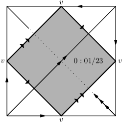
Figure 17: An edge link in the $1$-tetrahedron triangulation of the $3$-sphere—a torus consisting of a single quadrilateral.

Example 2 ((Quadrilateral surfaces with two vertices)).

Lemma 2 is also sharp for $v=2$ and arbitrary genus. For the $2$-vertex case consider the following family of $2g$-tetrahedra $3$-vertex $3$-spheres $\mathscr{B}_{g}$, $g\geq 2$, given by the following gluing table; here $i(abc)$ in row $j$, column $(def)$ means that triangle $(def)$ of tetrahedron $j$ is glued to triangle $(abc)$ of tetrahedron $i$. Each of the $\mathscr{B}_{g}$, $g\geq 2$, contains a quadrangulated genus $g$ splitting surface with only two vertices for all $g\geq 2$. The splitting surface is given by one quadrilateral per tetrahedron each separating vertices $0$ and $2$ from $1$ and $3$ and is shown in Figure 18.

tetrahedron	face $(012)$	face $(013)$	face $(023)$	face $(123)$
$0$	$0(032)$	$1(013)$	$0(021)$	$1(123)$
$1$	$2(012)$	$0(013)$	$2(023)$	$0(123)$
$2$	$1(012)$	$\ldots$	$1(023)$	$\ldots$
$\ldots$	$\ldots$	$\ldots$	$\ldots$	$\ldots$
$\ldots$	$\ldots$	$\ldots$	$\ldots$	$\ldots$
$2k-1$	$2k(012)$		$2k(023)$
$2k$	$2k-1(012)$	$2k+1(013)$	$2k-1(023)$	$2k+1(123)$
$2k+1$	$\ldots$	$2k(013)$	$\ldots$	$2k(123)$
$\ldots$	$\ldots$	$\ldots$	$\ldots$	$\ldots$
$\ldots$	$\ldots$	$\ldots$	$\ldots$	$\ldots$
$2g-3$	$2g-2(012)$	$\ldots$	$2g-2(023)$	$\ldots$
$2g-2$	$2g-3(012)$	$2g-1(013)$	$2g-3(023)$	$2g-1(123)$
$2g-1$	$2g-1(032)$	$2g-2(013)$	$2g-1(021)$	$2g-2(123)$

Figure 18: Genus $g$ splitting surface in $\mathscr{B}_{g}$ with only $2g$ quadrilaterals.

Example 3 ((Gale surfaces)).

The following construction describes a family of simplicial triangulations of the 3–sphere containing interesting quadrilateral surfaces. The cyclic $4$–polytope $C_{4}(n)$ with vertex set $V=\{0,1,\ldots,n-1\}$ is neighbourly, i. e. it contains all possible ${n\choose 2}$ edges. On the other hand, by Gale’s evenness condition, the span of all odd vertices $V_{1}=\{1,3,\ldots,n-1\}$ as well as the span of all even vertices $V_{2}=\{0,2,\ldots,n-2\}$ both have dimension $1$. Altogether, the normal surface $G_{n}$ separating $V_{1}$ from $V_{2}$ slices each of the ${n\choose 2}-n$ tetrahedra in the boundary of the polytope in a quadrilateral and has genus ${\frac{n}{2}-1\choose 2}$. As a consequence, $G_{n}$ has $\frac{n^{2}}{4}$vertices and the $f$-vector

$$f(G_{n})=\left(\frac{n^{2}}{4},2\left({n\choose 2}-n\right),{n\choose 2}-n\right).$$

Whence

$$g(G_{n})=\frac{n^{2}}{8}-\frac{3n}{4}+1=\frac{f_{0}(G_{n})}{2}-\frac{3\sqrt{f_{0}(G_{n})}}{2}+1.$$

We call the splitting surface $G_{n}$ a Gale surface (cf. [42]). It has the maximum genus with respect to $n$ and linear genus with a relatively large constant with respect to $f_{0}(G_{n})$. Furthermore, it is polyhedrally realisable in $\mathbb{R}^{3}$ by just adding four vertices in one quadrilateral disc (cf. Section 5).

Example 4 ((Simplicial triangulations)).

Given an $n$-vertex simplicial $3$-manifold triangulation $M$ containing a complete graph $K_{m}$ on $m$ vertices $m<n$ such that each edge in $K_{m}$ is of degree three in $M$. Then the boundary of a small neighborhood of $K_{m}$ is a normal surface $S$ of genus $g(S)={m-1\choose 2}$ consisting of $q(S)=3{m\choose 2}$ quadrilaterals and possibly a large number of triangles. Given an arbitrarily large number of vertices such a simplicial triangulationn $M$ is easy to construct: take a collection of cones over simplicial $2$-sphere triangulations with sufficiently many degree three vertices and pairwise join these cones together by identifying the star around a degree three edge, and finally closing off the resulting complex. Note that this family can also be extended to all values $g\geq 0$, $g(S)\neq{m-1\choose 2}$, by slightly modifying $M$. All together this results in in normal surfaces $S$ with

$$q(S)=3g(S)+O(\sqrt{g(S)}).$$

Despite an extended computer search using the classification of simplicial $3$-manifold triangulations with few vertices [2, 34] and the library of $3$-manifold triangulations contained in the GAP-package simpcomp [16] these examples of normal surfaces in simplicial triangulations have the least number of quadrilaterals for fixed $g\neq 2$ amongst all known examples. In the case $g=2$ there is an $8$-vertex $3$-manifold triangulation of $S^{3}$ containing a normal surface with only $14$ quadrilaterals where the above method would result in $15$ quadrilaterals.

It is thus conjectured that for normal surfaces in simplicial triangulations

$$q(S)\geq 3g(S)$$

holds [42].

6.2 Fundamental normal surfaces

Example 5 (($3q=2g$)).

Theorem 3 is sharp for $g=0$ and $g=3,$ and hence a sharp linear bound of genus in terms of quadrilateral discs.

• $g=0$: For this case consider any vertex linking sphere in a closed 3–manifold.

• $g=3$: The $6$-tetrahedra triangulation of the $3$-sphere given by below gluing table contains a genus $3$ vertex normal surface (in standard coordinates) with only two quadrilaterals, which is shown in Figure 19.

  tetrahedra	face $(012)$	face $(013)$	face $(023)$	face $(123)$
  $0$	$0(301)$	$0(120)$	$2(023)$	$1(123)$
  $1$	$3(012)$	$2(103)$	$2(123)$	$0(123)$
  $2$	$4(012)$	$1(103)$	$0(023)$	$1(023)$
  $3$	$1(012)$	$5(013)$	$4(123)$	$4(023)$
  $4$	$2(012)$	$5(203)$	$3(123)$	$3(023)$
  $5$	$5(231)$	$3(013)$	$4(103)$	$5(201)$

  

  Figure 19: A genus $3$ quadrilateral fundamental normal surface with only $2$ quadrilaterals.

Example 6 (($q=g$)).

For $g=1$ and $g=2$ there exist examples of orientable normal surfaces with the minimal number of quadrilaterals with respect to Theorem 3.

• $g=1$: For this case consider the $1$-quadrilateral torus inside the $1$-tetrahedron triangulation of the $3$-sphere from Example 1.

• $g=2$: There is a $4$-tetrahedra $0$-efficient $3$-sphere given by the following gluings.

  tetrahedra	face $(012)$	face $(013)$	face $(023)$	face $(123)$
  $0$	$3(012)$	$1(013)$	$2(023)$	$1(123)$
  $1$	$3(013)$	$0(013)$	$2(013)$	$0(123)$
  $2$	$3(231)$	$1(023)$	$0(023)$	$3(023)$
  $3$	$0(012)$	$1(012)$	$2(123)$	$2(201)$

  The triangulation contains a genus $2$ fundamental normal surface in quadrilateral coordinates with only two quadrilaterals which is shown in Figure 20.

Figure 20: A genus $2$ quadrilateral fundamental normal surface with only $2$ quadrilaterals.

Example 7 ((Non-orientable normal surface)).

The $5$-terahedra triangulation of $S^{2}\times S^{1}$ given by the gluing table

tetrahedra	face $(012)$	face $(013)$	face $(023)$	face $(123)$
$0$	$0(013)$	$0(012)$	$2(023)$	$1(123)$
$1$	$4(012)$	$4(013)$	$3(023)$	$0(123)$
$2$	$4(230)$	$4(231)$	$0(023)$	$3(123)$
$3$	$3(013)$	$3(012)$	$1(023)$	$2(123)$
$4$	$1(012)$	$1(013)$	$2(201)$	$2(301)$

contains a non-orientable vertex normal surface of Euler characteristic $-2$ with only $1$ quadrilateral. The surface is shown in Figure 21. Note that taking the orientable double cover of this surface yields a $2$ quadrilateral orientable surface of Euler characteristic $-4$, and hence another sharp example for Theorem 3.

Figure 21: A $1$ quadrilateral non-orientable normal surface of Euler characteristic $-2$.

Example 8 (($g=q$)).

The family of triangulations $\mathscr{A}_{n}$ given in [12] provides examples of normal surfaces of arbitrary $g\geq 1$ each with few quadrilaterals with respect to their genus. It consists of a cycle of $n$ tetrahedra, each identified with itself around a degree one edge and joined to each other along the remaining triangles such that all vertices become identified. For all $n\geq 1$, the triangulation $\mathscr{A}_{n}$ is a $1$–vertex $0$–efficient triangulation of the $3$–sphere.

The triangulation $\mathscr{A}_{n}$ contains exactly ${n\choose k}$ genus $k$ normal surfaces, each having $k$ quadrilaterals dual to $k$ of the $n$ edges of degree one. In particular, there is a genus $n$ normal surface containing exactly $n$ quadrilaterals.

In standard coordinates all of these surfaces are fundamental normal surfaces. However, the $n$ quadrilateral genus $n$ normal surface is the sum of $n$ fundamental tori minus $(n-1)$ copies of the vertex link; so it is not fundamental in $Q$–coordinates.

Example 9 ((Normal surface with boundary)).

There is a $4$-tetrahedra triangulation of the $3$-ball containing a $2$-punctured torus with only one quadrilateral and thus an example of equality in Corollary 5 ($g=1$, $b=2$, and $q=1$). The triangulation is given by the following gluing table, where $\partial$ denotes a triangle in the boundary. The $2$-punctured torus is shown in Figure 22.

tetrahedra	face $(012)$	face $(013)$	face $(023)$	face $(123)$
$0$	$0(013)$	$0(012)$	$\partial$	$1(123)$
$1$	$3(012)$	$3(013)$	$2(023)$	$0(123)$
$2$	$2(013)$	$2(012)$	$1(023)$	$\partial$
$3$	$1(012)$	$1(013)$	$3(312)$	$3(230)$

Figure 22: A $2$-punctured torus ($b=2$, $g=1$) with only one quadrilateral.

Example 10 ((A non-trivial Haken sum with $g=5$ and $q=4$)).

Consider the following $8$-tetrahedra triangulation $M$ of $S^{2}\times S^{1}$:

tetrahedra	face $(012)$	face $(013)$	face $(023)$	face $(123)$
$0$	$3(012)$	$1(013)$	$2(023)$	$1(123)$
$1$	$4(132)$	$0(013)$	$4(023)$	$0(123)$
$2$	$3(032)$	$5(013)$	$0(023)$	$3(321)$
$3$	$0(012)$	$6(013)$	$2(021)$	$2(321)$
$4$	$7(120)$	$7(013)$	$1(023)$	$1(021)$
$5$	$6(032)$	$2(013)$	$6(021)$	$7(320)$
$6$	$5(032)$	$3(013)$	$5(021)$	$7(123)$
$7$	$4(201)$	$4(013)$	$5(321)$	$6(123)$

$M$ contains a one quadrilateral non-orientable surface $\mathbf{s}_{1}$ of non-orientable genus $4$ with coordinates

$$\begin{array}[]{rcl}\mathbf{s}_{1}&=(&(0,0,0,0;0,1,0),(1,0,1,0;0,0,0),(0,0,0,1;0,0,0),(0,1,0,0;0,0,0),\\ &&(1,1,1,0;0,0,0),(0,0,1,1;0,0,0),(0,1,1,0;0,0,0),(1,1,1,0;0,0,0)\quad),\end{array}$$

as well as a two quadrilateral orientable surface $\mathbf{s}_{2}$ of genus $3$ with coordinates

$$\begin{array}[]{rcl}\mathbf{s}_{2}&=(&(0,1,0,1;0,1,0),(1,1,1,1;0,0,0),(0,0,0,2;0,0,0),(0,2,0,0;0,0,0),\\ &&(1,1,1,1;0,0,0),(0,0,0,2;0,0,0),(0,2,0,0;0,0,0),(1,1,0,0;1,0,0)\quad).\end{array}$$

Hence, both $\mathbf{s}_{1}$ and $\mathbf{s}_{2}$ attain equality in Corollary 4 and Theorem 3 respectively. Moreover, $\mathbf{s}_{1}$ and $\mathbf{s}_{2}$ are compatible, non-disjoint and the sum of the orientable double cover of $\mathbf{s}_{1}$ together with $\mathbf{s}_{2}$ is connected. It follows that $2\mathbf{s}_{1}+\mathbf{s}_{2}$ is a non-trivial example for which the bound from Corollary 7 is sharp.

$2\mathbf{s}_{1}+\mathbf{s}_{2}$ has $48$ triangles, $4$ quadrilaterals and genus $5$. It is shown in Figure 23.

Figure 23: A non-trivial Haken sum genus five surface with only four quadrilaterals.

6.3 Incompressible surfaces

Incompressible surfaces are extremely hard to find because checking for incompressibility requires running an algorithm with a doubly exponential worst case running time. However, the fourth author and others were able to obtain a complete classification of all incompressible surfaces of the $11031$ triangulations from the Hodgson-Weeks census by running extensive computer experiments [10]. As a result, there are $36449$ incompressible quad vertex normal surfaces, $19696$ of which are injective and $16753$ which occur as a double cover of a non-orientable vertex normal surface. All incompressible surfaces have genus $2\leq g\leq 5$ and none of them attains equality in Corollary 8. However, some of them have only few more quadrilaterals than necessary. Comparing the number of quadrilaterals in these surfaces to the number of quadrilaterals in the complete set of $441331$ quad vertex normal surfaces of genus $2\leq g\leq 5$ in the census reveals a slightly higher average number of quadrilaterals amongst the incompressible surfaces as can be seen in the following table.

	injective essential surfaces				double covers
genus	# surfaces	$\min_{s}q(S)$	$\overline{q(S)}$	$\max_{S}q(S)$	# surfaces	$\min_{S}q(S)$	$\overline{q(S)}$	$\max_{S}q(S)$
$2$	$16622$	$6$	$20$	$90$	$11711$	$6$	$23$	$114$
$3$	$3023$	$15$	$34$	$109$	$4598$	$14$	$44$	$226$
$4$	$46$	$27$	$48$	$85$	$355$	$24$	$61$	$166$
$5$	$5$	$36$	$43$	$56$	$89$	$32$	$55$	$98$
	all essential surfaces				all (orientable) vertex surfaces
genus	# surfaces	$\min_{S}q(S)$	$\overline{q(S)}$	$\max_{S}q(S)$	# surfaces	$\min_{S}q(S)$	$\overline{q(S)}$	$\max_{S}q(S)$
$2$	$28333$	$6$	$21$	$114$	$268202$	$5$	$13$	$100$
$3$	$7621$	$14$	$40$	$226$	$120844$	$7$	$22$	$187$
$4$	$401$	$24$	$59$	$166$	$37877$	$13$	$33$	$205$
$5$	$94$	$32$	$55$	$98$	$14408$	$19$	$42$	$200$

The complete data for all quad vertex normal surfaces compared to the incompressible surfaces of $2\leq g\leq 4$ in the census is summarised by Figure 24.

Figure 24: Number of quads in the incompressible surfaces (left) and in all quad vertex normal surfaces (right) of the Hodgson-Weeks census.

Example 11 ((Incompressible surfaces with $q=2g$)).

By construction, the separating surfaces used in Section 4.2 to show that $c(S_{g}\times I)\leq 10g-4$, are incompressible and have exactly $2g$ quadrilaterals each. Hence, the bound presented in Corollary 8 is sharp for all values $g\geq 1$.

Below we present the case $g=1$ where the two quadrilateral incompressible torus lives inside the minimal trivial torus bundle $T^{2}\times S^{1}$ which can be obtained from the six tetrahedra triangulation of $S_{g}\times I$ by identifying its two boundary components (cf. Figure 25).

tetrahedra	face $(012)$	face $(013)$	face $(023)$	face $(123)$
$0$	$4(012)$	$3(013)$	$2(023)$	$1(123)$
$1$	$3(320)$	$4(230)$	$5(023)$	$0(123)$
$2$	$3(231)$	$4(321)$	$0(023)$	$5(123)$
$3$	$5(103)$	$0(013)$	$1(210)$	$2(201)$
$4$	$0(012)$	$5(102)$	$1(301)$	$2(310)$
$5$	$4(103)$	$3(102)$	$1(023)$	$2(123)$

Figure 25: A $2$ quadrilateral incompressible torus.

References

- [1] A. Altshuler. Polyhedral realization in of triangulations of the torus and -manifolds in cyclic -polytopes. Discrete Math., 1, (1971/1972), no. 3, 211–238.
- [2] A. Altshuler. Combinatorial -manifolds with few vertices. J. Combinatorial Theory Ser. A, 16:165–173, 1974.
- [3] D. Archdeacon, C. P. Bonnington, and J. A. Ellis-Monaghan. How to exhibit toroidal maps in space. Discrete Comput. Geom., 38 (2007), no. 3, 573–594.
- [4] J. Bokowski. On heuristic methods for finding realizations of surfaces. In Discrete differential geometry, volume 38 of Oberwolfach Semin., Birkhäuser, Basel, (2008), 255–260.
- [5] J. Bokowski and U. Brehm. A new polyhedron of genus with vertices. In Intuitive geometry (Siófok, 1985). Volume 48 of Colloq. Math. Soc. János Bolyai. North-Holland, Amsterdam, (1987), 105–116.
- [6] J. Bokowski and A. Eggert. Toutes les réalisations du tore de Möbius avec sept sommets. Structural Topology, 17, (1991), 59–78.
- [7] B. A. Burton: Face pairing graphs and 3-manifold enumeration, J. Knot Theory Ramifications 13 (2004), no. 8, 1057–1101.
- [8] B. A. Burton: Enumeration of non-orientable 3-manifolds using face-pairing graphs and union-find, Discrete Comput. Geom. 38 (2007), no. 3, 527–571.
- [9] B. A. Burton, R. Budney, W. Pettersson, et al.: Regina: Software for 3-manifold topology and normal surface theory, http://regina.sourceforge.net/, 1999–2012.
- [10] B. Burton, A. Coward, S. Tillmann. Computing closed essential surfaces in knot complements. In Proceedings of the 29th Annual Symposium on Computational Geometry, (2013), 405–414.
- [11] B. Burton and M. Ozlen. A tree traversal algorithm for decision problems in knot theory and 3-manifold topology. Algorithmica, 65(4), (2013), 772–801.
- [12] B. Burton, J. Paixao and J. Spreer. Computational topology and normal surfaces: Theoretical and experimental complexity bounds. In Proceedings of the 15th Meeting on Algorithm Engineering and Experiments, (2013), 78–87.
- [13] D. Cooper and S. Tillmann: The Thurston norm via normal surfaces. Pacific J. Math. 239 (2009), no. 1, 1–15.
- [14] Á. Császár. A polyhedron without diagonals. Acta Univ. Szeged. Sect. Sci. Math., 13, (1949), 140–142.
- [15] R. A. Duke. Geometric embedding of complexes. Amer. Math. Monthly, 77, (1970), 597–603.
- [16] F. Effenberger and J. Spreer. simpcomp - a GAP package, Version 2.0.0. https://code.google.com/p/simpcomp, 2013.
- [17] E. Fominykh and A. Vesnin. Exact values of complexity for Paoluzzi–Zimmermann manifolds (Russian). Dokl. Akad. Nauk 439 (2011), no. 6, 727–729. Translation in Dokl. Math. 84 (2011), no. 1, 542–544.
- [18] R. Frigerio, B. Martelli, C. Petronio. Complexity and Heeagaard genus of an infinite class of compact 3-manifolds, Pacific J. Math. 210, (2003), 283–297.
- [19] B. Grünbaum. Convex polytopes. Volume 221 of Graduate Texts in Mathematics. Springer-Verlag, New York, second edition, (2003). Prepared and with a preface by Volker Kaibel, Victor Klee and Günter M. Ziegler.
- [20] W. Haken. Theorie der Normalflächen. Acta Math., 105, (1961), 245–375.
- [21] W. Haken. Über das Homöomorphieproblem der –Mannigfaltigkeiten. I, Math. Z., 80, (1962), 89–120.
- [22] J. Hass, J. C. Lagarias, and N. Pippenger. The computational complexity of knot and link problems. J. ACM 46, (1999), no. 2, 185–211.
- [23] G. Hemion: On the classification of homeomorphisms of 2–manifolds and the classification of 3–manifolds. Acta Math. 142 (1979), no. 1-2, 123–155.
- [24] S. Hougardy, F. H. Lutz, and M. Zelke. Surface realization with the intersection segment functional. Experiment. Math., 19, (2010), no. 1, 79–92.
- [25] W. Jaco and U. Oertel. An algorithm to decide if a 3-manifold is a Haken manifold. Topology 23 (1984), no. 2, 195–209.
- [26] W. Jaco and J. H. Rubinstein. 0–efficient triangulations of 3–manifolds. Journal of Differential Geometry 65, (2003), no. 1, 61–168.
- [27] W. Jaco and J. .H. Rubinstein. Inflations of ideal triangulations. Advances in Mathematics 267, (2014) 176–224.
- [28] W. Jaco, J. H. Rubinstein and S. Tillmann. Minimal triangulations for an infinite family of lens spaces. Journal of Topology 2, (2009), no. 1, 157–180.
- [29] W. Jaco, J. H. Rubinstein and S. Tillmann. Coverings and minimal triangulations of -manifolds. Algebr. Geom. Topol., 11, (2011), no. 3, 1257–1265.
- [30] T. Kalelkar. Euler characteristic and quadrilaterals of normal surfaces. Proc. Indian Acad. Sci. Math. Sci., 118, (2008), no. 2, 227–233.
- [31] H. Kneser. Geschlossene Flächen in dreidimensionalen Mannigfaltigkeiten. Jahresbericht der deutschen Mathematiker-Vereinigung, 38, (1929), 248–260.
- [32] F. Luo and S. Tillmann: Triangulated 3-Manifolds: Combinatorics and Volume Optimisation, arXiv:1312.5087.
- [33] F. H. Lutz. Enumeration and random realization of triangulated surfaces. In Discrete differential geometry, volume 38 of Oberwolfach Semin., Birkhäuser, Basel, (2008), 235–253.
- [34] F. H. Lutz. The Manifold Page. http://www.math.tu-berlin.de/diskregeom/stellar.
- [35] S. V. Matveev. Complexity theory of three-dimensional manifolds. Acta Appl. Math. 19, (1990), no. 2, 101–130.
- [36] S. Matveev: Algorithmic topology and classification of 3-manifolds. Algorithms and Computation in Mathematics, 9. Springer-Verlag, Berlin, 2003.
- [37] P. McMullen, C. Schulz, and J. M. Wills. Polyhedral -manifolds in with unusually large genus. Israel J. Math., 46, (1983), no. 1–2, 127–144.
- [38] G. Ringel. Map color theorem. Volume 209 of Die Grundlehren der mathematischen Wissenschaften. Springer-Verlag, New York, (1974).
- [39] J. H. Rubinstein. An algorithm to recognize the 3–sphere. In Proceedings of the International Congress of Mathematicians (Zürich, 1994), volume 1, Birkhäuser, Basel, (1995), 601–611.
- [40] J. H. Rubinstein. Polyhedral minimal surfaces, Heegaard splittings and decision prob- lems for 3–dimensional manifolds. In Geometric Topology (Athens, GA, 1993). AMS/IP Stud. Adv. Math. 2, Amer. Math. Soc. (1997), 1–20.
- [41] L. Schewe. Nonrealizable minimal vertex triangulations of surfaces: showing nonrealizability using oriented matroids and satisfiability solvers. Discrete Comput. Geom., 43, (2010), no. 2, 289–302.
- [42] J. Spreer. Normal surfaces as combinatorial slicings. Discrete Math., 311, (2011), no. 14, 1295–1309.
- [43] E. Steinitz. Über die Eulerschen Polyederrelationen. Arch. der Math. u. Phys., 11, (1906), no. 3, 86–88.
- [44] A. Thompson. Thin position and the recognition problem for , Math. Res. Lett. 1, (1994), 613–630.
- [45] S. Tillmann. Normal surfaces in topologically finite 3–manifolds, L’Enseignement Mathématique, 54, (2008), no. 2, 329–380.
- [46] J. L. Tollefson. Normal surface –theory, Pacific J. of Math., 183, (1998), 359–374.
- [47] G. M. Ziegler. Polyhedral surfaces of high genus. In Discrete differential geometry, volume 38 of Oberwolfach Semin., Birkhäuser, Basel, (2008), 191–213.