Vector meson spectral function and dilepton production rate in a hot and dense medium within an effective QCD approach

Abstract

The properties of the vector meson current-current correlation function and its spectral representation are investigated in details with and without isoscalar-vector interaction within the framework of effective QCD approach, namely Nambu$\textendash$Jona-Lasinio (NJL) model and its Polyakov Loop extended version (PNJL), at finite temperature and finite density. The influence of the isoscalar-vector interaction on the vector meson correlator is obtained using the ring resummation known as the Random Phase Approximation (RPA). The spectral as well as the correlation function in PNJL model show that the vector meson retains its bound property up to a moderate value of temperature above the phase transition. Using the vector meson spectral function we, for the first time, obtained the dilepton production rate from a hot and dense medium within the framework of PNJL model that takes into account the nonperturbative effect through the Polyakov Loop fields. The dilepton production rate in PNJL model is enhanced compared to NJL and Born rate in the deconfined phase due to the suppression of color degrees of freedom at moderate temperature. The presence of isoscalar-vector interaction further enhances the dileption rate over the Born rate in the low mass region. Further, we also have computed the Euclidean correlation function in vector channel and the conserved density fluctuation associated with temporal correlation function appropriate for a hot and dense medium. The dilepton rate and the Euclidean correlator are also compared with available lattice data and those quantities in PNJL model are found to agree well in certain domain.

1 Introduction

Quantum Chromodynamics (QCD) being the fundamental theory of strong interaction exhibits a very rich phase structure at extreme conditions, i.e., high temperature and/or high density. It is now well established that at these conditions a transition from normal hadronic matter to a state of strongly interacting exotic quark gluon plasma (QGP) is possible Muller:1983ed ; Heinz:2000bk . In recent years, a tremendous effort has been devoted to the creation of QGP in the laboratory. The heavy-ion collider experiments presently dedicated to this search are the Relativistic Heavy Ion Collider (RHIC) at Brookhaven National Laboratory (BNL) Arsene:2004fa ; Back:2004je ; Adams:2005dq ; Adcox:2004mh and the Large Hadron Collider (LHC) at the European Organization for Nuclear Research (CERN) Carminati:2004fp ; Alessandro:2006yt . Also, future fixed target experiments are planned at the Facility for Antiproton and Ion Research (FAIR) at the Gesellschaft für Schwerionenforschung (GSI) Friman:2011zz . In all these experiments heavy ions are accelerated to relativistic speeds in order to achieve such extreme conditions required for the creation of a short-lived QGP. Various diagnostic measurements at RHIC BNL Adare:2009qk ; Adler:2006yt ; Adare:2006ti ; Adcox:2001jp ; Adcox:2002au ; Adler:2003kg ; Chujo:2002bi ; Adare:2006nq ; Abelev:2006db in the recent past have indicated a strong hint for the creation of a semi-QGP (not weakly interacting like usual QGP) within a first few fm/$c$ of the collisions through the manifestation of hadronic final states. Also, new data from LHC CERN Aamodt:2010pb ; Aamodt:2010pa ; Aamodt:2010jd ; Aad:2010bu ; Chatrchyan:2011sx have further consolidated the formation of such a state of matter.

One of the most interesting as well as promising subjects in the area of theoretical high energy physics is the study of the strongly interacting many particle system under these extreme conditions. Dynamical properties of many particle system are associated with the correlation function Forster(book):1975HFBSCF ; Callen:1951vq ; Kubo:1957mj . We know that many of the hadron properties are embedded in the correlation function and its spectral representation. Such properties in vacuum Davidson:1995fq are very well studied in QCD. The presence of a stable mesonic state is understood by the delta function like peak in the spectral function. At low temperature most of the hadronic models Andronic:2012ut ; Huovinen:2009yb work well but break down near the phase transition temperature, $T_{c}$. While propagating through the hot and dense medium Kapusta_Gale(book):1996FTFTPA ; Lebellac(book):1996TFT , the vacuum properties of any particle get modified due to the change of its dispersion properties in the medium. The temporal correlation function is related to the response of the conserved density fluctuations due to the symmetry of the system. On the other hand, the spatial correlation function exhibits information on the masses and width. So, in a hot and dense medium the properties of hadrons, viz., response to the fluctuations, masses, width, compressibility etc., will be affected. Hence, hadron properties at finite temperature and density are also encoded in the structure of its correlation function and the corresponding spectral representation, which may reflect the degrees of freedom around the phase transition point and thus the properties of the deconfined, strongly interacting matter. As for example, the spectral representation of the vector current-current correlation can be indirectly accessible by high energy heavy-ion experiments as it is related to the differential thermal cross section for the production of lepton pairs Kapusta_Gale(book):1996FTFTPA ; Lebellac(book):1996TFT . Moreover, in the limit of small frequencies, various transport coefficients of the hot and dense medium can be determined from the spatial spectral representation of the vector channel correlation Kapusta_Gale(book):1996FTFTPA ; Lebellac(book):1996TFT . The static limit of the temporal correlation function provides the response to the fluctuation of the conserved quantities. For a quasiparticle in the medium, the $\delta$-like peak is expected to be smeared due to the thermal width, which increases with the increase in temperature. At sufficiently high temperature and density, the contribution from the mesonic state in the spectral function will be broad enough so that it is not very meaningful to speak of it as a well defined state any more Gale:1990pn ; Mustafa:1999dt ; Ghosh:2009bt .

At high temperature but zero chemical potential, the structure of the vector meson correlation function, determination of thermal dilepton rate and various transport coefficients have been studied using Lattice QCD (LQCD) framework at zero momentum Ding:2010ga ; Kaczmarek:2011ht ; Francis:2011bt ; Datta:2003ww ; Aarts:2007wj ; Aarts:2002cc ; Aarts:2002tn ; Amato:2013naa ; Karsch:2001uw and also at nonzero momentum Aarts:2005hg , which is a first principle calculation that takes into account the nonperturbative effects of QCD. Such studies for hot and dense medium are also performed within perturbative techniques like Hard Thermal Loop (HTL) approximation Karsch:2000gi ; Braaten:1990wp ; Greiner:2010zg ; Chakraborty:2003uw ; Chakraborty:2001kx ; Chakraborty:2002yt ; Laine:2011xm ; Czerski:2008zz ; Czerski:2006ct ; Alberico:2006wc ; Alberico:2004we ; Arnold:2000dr ; Arnold:2003zc ; Burnier:2012ze , and in dimensional reduction Laine:2003bd ; Hansson:1991kb appropriate for weakly interacting QGP. Nevertheless, at RHIC and LHC energies the maximum temperature reached is not very far from the phase transition temperature $T_{c}$ and a hot and dense matter created in these collisions is nonperturbative in nature (semi-QGP). So, most of the perturbative methods may not be applicable in this temperature domain but these methods, however, are very reliable and accurate at very high temperature Haque:2013sja ; Haque:2014rua ; Haque:2013qta ; Haque:2012my for usual weakly interacting QGP. In effective QCD model framework Gale:1990pn ; Mustafa:1999dt ; He:2003jza ; He:2002pv ; He:2002ii ; Kunihiro:1991qu ; Oertel:2000jp , several studies have also been done in this direction. Mesonic spectral functions and the Euclidean correlator in scalar, pseudoscalar and vector channel have been discussed in Refs. He:2003jza ; He:2002pv ; He:2002ii ; Kunihiro:1991qu ; Oertel:2000jp using Nambu$\textendash$Jona-Lasinio (NJL) model. The NJL model has no information related to the confinement and thus does not have any nonperturbative effect associated with the semi-QGP above $T_{c}$. However, the Polyakov Loop extended NJL (PNJL) model Fukushima:2003fw ; Fukushima:2003fm contains nonperturbative information through Polyakov Loop Pisarski:2000eq ; Dumitru:2001xa ; Dumitru:2002cf ; Dumitru:2003hp ; Gross:1980br ; Gocksch:1993iy ; Weiss:1980rj ; Weiss:1981ev that suppresses the color degrees of freedom as the Polyakov Loop expectation value decreases when $T\rightarrow T_{c}^{+}$. The thermodynamic properties of strongly interacting matter have been studied extensively within the framework of NJL and PNJL models Ghosh:2006qh ; Mukherjee:2006hq ; Ghosh:2007wy ; Ratti:2005jh ; Ghosh:2014zra . The properties of the mesonic correlation functions have also been studied in scalar and pseudoscalar channel using PNJL model in Refs. Hansen:2006ee ; Deb:2009ng . We intend to study, for the first time in PNJL model, the properties of the vector correlation function and its spectral representation to understand the nonperturbative effect on the spectral properties, e.g., the dilepton production rate and the conserved density fluctuations, in a hot and dense matter created in heavy-ion collisions.

Further, the low temperature and high density part of the phase diagram is still less explored compared to the high temperature one. At finite densities the effect of chirally symmetric vector channel interaction becomes important and it is established that within the NJL or PNJL model this type of interaction weakens the first order transition line Carignano:2010ac ; Kashiwa:2006rc ; Sakai:2008ga ; Fukushima:2008wg ; Fukushima:2008is ; Denke:2013jmp in contrary to the scalar coupling which tends to favor the appearance of first order phase transitions. It is important to mention here that the determination of the strength of vector coupling constant is crucial under model formalism. It cannot be fixed using vector meson mass as it is beyond the characteristic energy cut-off of the model. However, at the same time incorporation of vector interaction is important if one intends to study the various spectral properties of the system at non-zero chemical potential Kunihiro:1991qu ; Jaikumar:2001jq appropriate for FAIR scenario Friman:2011zz . In the present work, we study the nonperturbative effect of Polyakov Loop, along with the presence as well as the absence of the repulsive isoscalar-vector interaction, on the spectral function, correlation function and various spectral properties, (e.g., the rate of dilepton production, fluctuation of conserved charges) in a hot and dense matter. The influence of this repulsive vector channel interaction on the correlator and its spectral representation has been obtained using ring resummation. The results are compared with NJL model and the available lattice QCD (LQCD) data.

The paper is organized as follows: in Sec. 2 we will briefly outline some of the generalities related to the correlation function and its spectral representation, and their relations to various physical quantities we would like to study. In Sec. 3 we briefly sketch the effective models namely NJL and PNJL model. In Sec. 4 we obtain the vector correlation function and its spectral properties through the isoscalar-vector interaction within the ring resummation both in vacuum as well as in a hot and dense medium. We present our findings relevant for a hot and dense medium in Sec. 5 and finally, conclude in Sec. 6.

2 Some Generalities

2.1 Correlation Function and its Spectral Representation

In general the correlation function in coordinate space is given by

$${\cal G}_{AB}(t,{\vec{x}})\equiv{\cal T}({\hat{A}}(t,{\vec{x}}){\hat{B}}(0,{\vec{0}}))=\int\frac{d\omega}{2\pi}\int\frac{d^{3}{q}}{(2\pi)^{3}}\ \ e^{i\omega t-i{\vec{q}}\cdot{\vec{x}}}\ \ {\cal G}_{AB}(\omega,{\vec{q}}),$$ (1)

where ${\cal T}$ is the time-ordered product of the two operators $\hat{A}$ and $\hat{B}$, and the four momentum $Q\equiv(\omega,{\vec{q}})$ with $q=|{\vec{q}}|$.

By taking the Fourier transformation one can obtain the momentum space correlation function as

$${\cal G}_{AB}(\omega,{\vec{q}}) = \int dt\int d^{3}{\vec{x}}\ \ {\cal G}_{AB}(t,{\vec{x}})\ \ e^{-i\omega t+i{\vec{q}}\cdot{\vec{x}}}\ \ .$$ (2)

The thermal meson current-current correlator in Euclidean time $\tau\in$ [$0,\ \beta=1/T$] is given as Karsch:2000gi ; Haque:2011iz

$${\cal G}^{E}_{M}(\tau,{\vec{x}})=\langle{\cal T}(J_{M}(\tau,{\vec{x}})J_{M}^{\dagger}(0,{\vec{0}}))\rangle_{\beta}=T\sum_{n=-\infty}^{\infty}\int\frac{d^{3}q}{(2\pi)^{3}}\ e^{-i(\omega_{n}\tau+{\vec{q}}\cdot{\vec{x}})}\ {\cal G}^{E}_{M}(i\omega_{n},{\vec{q}}),$$ (3)

where the mesonic current is defined as $J_{M}={\bar{\psi}}(\tau,{\vec{x}})\Gamma_{M}\psi(\tau,{\vec{x}})$, with $\Gamma_{M}$ =$1,\gamma_{5},\gamma_{\mu},\gamma_{\mu}\gamma_{5}$ for scalar, pseudoscalar, vector and pseudovector channel respectively. The momentum space correlator ${\cal G}^{E}_{M}(i\omega_{n},\vec{q})$ at the discrete Matsubara modes $\omega_{n}=2\pi nT$ can be obtained as

$${\cal G}^{E}_{M}(i\omega_{n},\vec{q})=-\int_{-\infty}^{\infty}d\omega\ \ \frac{\sigma_{M}(\omega,\vec{q})}{i\omega_{n}-\omega}.$$ (4)

The spectral function $\sigma_{H}(\omega,\vec{q})$ for a given mesonic channel $H$, can be obtained from the imaginary part of the momentum space Euclidean correlator in (4) by analytic continuation as

$$\sigma_{H}(\omega,\vec{q}) = \frac{1}{\pi}{\mbox{Im}}\ {\cal G}^{E}_{H}(i\omega_{n}=\omega+i\epsilon,\vec{q}),$$ (5)

where $H=00,ii$ and $V$ stand for temporal, spatial and vector spectral function, respectively. The vector spectral function is expressed in terms of temporal and spatial components as ${\rm\sigma_{V}}=\sigma_{00}-\sigma_{ii}$.

Using (3) and (4) one obtains the spectral representation of the thermal correlation function in Euclidean time but at a fixed momentum $\vec{q}$ as

$${\cal G}^{E}_{H}(\tau,\vec{q})=\int_{0}^{\infty}\ d\omega\ \sigma_{H}(\omega,\vec{q})\ \frac{\cosh[\omega(\tau-\beta/2)]}{\sinh[\omega\beta/2]}.$$ (6)

Because of the difficulty in analytic continuation in LQCD the spectral function can not be obtained directly using (5). Instead a calculation in LQCD proceeds by evaluating the Euclidean correlation function. Using a probabilistic application based on maximum entropy method (MEM) Nakahara:1999vy ; Asakawa:2000tr ; Wetzorke:2000ez , (6) is then inverted to extract the spectral function and thus various spectral properties are computed in LQCD.

2.2 Vector Spectral Function and Dilepton Rate

The vector meson spectral function, $\sigma_{V}$, and the differential dilepton production rate are related as Karsch:2000gi

$$\frac{dR}{d^{4}xd^{4}Q}=\frac{5\alpha^{2}}{54\pi^{2}}\frac{1}{M^{2}}\ \frac{1}{e^{\omega/T}-1}\ \sigma_{V}(\omega,{{\vec{q}}})\ ,$$ (7)

where the invariant mass of the lepton pair is $M^{2}=\omega^{2}-q^{2}$ and $\alpha$ is the fine structure constant.

2.3 Temporal Euclidean Correlation Function and Response to Conserved Density Fluctuation

The quark number susceptibility (QNS), $\chi_{q}$ measures of the response of the quark number density $\rho$ with infinitesimal change in the quark chemical potential, $\mu+\delta\mu$ and is related to temporal correlation function through fluctuation dissipation theorem Kunihiro:1991qu as

$$\chi_{q}(T) = \!\!\left.\frac{\partial\rho}{\partial\mu}\right|_{\mu=0}\!\!=\!\!\!\int\ d^{4}x\ \left\langle J_{0}(0,{\vec{x}})J_{0}(0,{\vec{0}})\right\rangle\$$ (8)

$$= {\lim_{\vec{q}\rightarrow 0}}\ \beta\int\frac{d\omega}{2\pi}\frac{-2}{1-e^{-\omega/T}}{\mbox{Im}}{\cal G}_{00}(\omega,{{\vec{q}}})=-{\lim_{\vec{q}\rightarrow 0}}{\mbox{Re}}\ {\cal G}_{00}(\omega=0,\vec{q}),$$

where Kramers-Kronig dispersion relation has also been used.

The quark number conservation implies that ${\lim_{\vec{q}\rightarrow 0}}{\mbox{Im}}{\cal G}_{00}(\omega,{\vec{q}})\propto\delta(\omega)$ and the temporal spectral function in (5) becomes

$$\sigma_{00}(\omega,{\vec{0}})=\frac{1}{\pi}{\mbox{Im}}{\cal G}_{00}(\omega,{\vec{0}})=-\omega\delta(\omega)\chi_{q}(T).$$ (9)

The relation of the Euclidean temporal correlation function and the response to the fluctuation of conserved number density, $\chi_{q}$, can be obtained from (6) as

$${\cal G}_{00}^{E}(\tau T)=-T\chi_{q}(T),$$ (10)

which is independent of the Euclidean time, $\tau$, but depends on $T$.

3 Effective QCD Models

3.1 NJL Model

In the present work we consider 2 flavor NJL model with vector channel interaction. The corresponding Lagrangian is Kunihiro:1991qu ; Klevansky:1992qe ; Hatsuda:1994pi ; Buballa:2003qv ; Davidson:1995fq :

$$\mathcal{L}_{\rm{NJL}}=\bar{\psi}(i\gamma_{\mu}\partial^{\mu}-m_{0})\psi+\frac{G_{S}}{2}[(\bar{\psi}\psi)^{2}+(\bar{\psi}i\gamma_{5}\vec{\tau}\psi)^{2}]-\frac{G_{V}}{2}(\bar{\psi}\gamma_{\mu}\psi)^{2},$$ (11)

where, $m_{0}=$diag$(m_{u},m_{d})$ with $m_{u}=m_{d}$ and $\vec{\tau}$’s are Pauli matrices. $G_{S}$ and $G_{V}$ are the coupling constants of local scalar type four-quark interaction and isoscalar-vector interaction respectively.

The scalar four quark interaction term leads to the formation of chiral condensate $\sigma=\langle\bar{\psi}\psi\rangle$. The condensate resulting from the additional vector coupling term only contains the time like component and the corresponding condensate is $n=\langle\bar{\psi}\gamma^{0}\psi\rangle$ Buballa:2003qv ; Kashiwa:2006rc . The thermodynamic potential in mean field approximation is given as:

$$\Omega_{\rm{NJL}} = \frac{G_{S}}{2}\sigma^{2}-\frac{G_{V}}{2}n^{2}-2N_{f}N_{c}\int_{\Lambda}\frac{d^{3}p}{(2\pi)^{3}}E_{p}$$ (12)

$$- 2N_{f}N_{c}T\int\frac{d^{3}p}{(2\pi)^{3}}\left[{\rm{ln}}(1+e^{-(E_{p}-\tilde{\mu})/T)}+{\rm{ln}}(1+e^{-(E_{p}+\tilde{\mu})/T)}\right].$$

Here $E_{p}=\sqrt{{\vec{p}}^{2}+M_{f}^{2}}$ is the energy of a quark with flavor $f$ having constituent mass or the dynamical mass $M_{f}$ and $\Lambda$ is a finite three momentum cut-off. The thermodynamic potential depends on the dynamical fermion mass $M_{f}$ and the modified quark chemical potential $\tilde{\mu}$ which are related to the scalar ($\sigma$) and vector ($n$) condensates through the relations

$$M_{f}=m_{0}-G_{S}\sigma,$$ (13)

and

$$\tilde{\mu}=\mu-G_{V}n,$$ (14)

respectively.

3.2 PNJL Model

Let us now briefly discuss PNJL model Ghosh:2006qh ; Mukherjee:2006hq ; Ghosh:2007wy ; Ratti:2005jh ; Fukushima:2008wg ; Ghosh:2014zra , where, unlike NJL model we have a couple of more mean fields in the form of the expectation value of the Polyakov Loop fields  $\Phi$ and its conjugate $\bar{\Phi}$. The Lagrangian for the 2 flavor PNJL model with vector channel interaction is given by,

$${\mathcal{L}}_{\rm PNJL} = \bar{\psi}(i\not{D}-m_{0}+\gamma_{0}\mu)\psi+\frac{G_{S}}{2}[(\bar{\psi}\psi)^{2}+(\bar{\psi}i\gamma_{5}\vec{\tau}\psi)^{2}]-\frac{G_{V}}{2}(\bar{\psi}\gamma_{\mu}\psi)^{2}$$ (15)

$$- {\mathcal{U}}(\Phi[A],\bar{\Phi}[A],T),$$

where $D^{\mu}=\partial^{\mu}-ig{\mathcal{A}}^{\mu}_{a}\lambda_{a}/2$, ${\mathcal{A}}^{\mu}_{a}$ being the $SU(3)$ background fields and $\lambda_{a}$’s are the Gell-Mann matrices. The thermodynamic potential can be obtained as Ghosh:2006qh ; Mukherjee:2006hq ; Ghosh:2007wy ; Ratti:2005jh

$${\Omega}_{\textrm{PNJL}} = {\mathcal{U}}(\Phi,{\bar{\Phi}},T)+\frac{G_{S}}{2}\sigma^{2}-\frac{G_{V}}{2}n^{2}$$ (16)

$$- 2N_{f}T\int\frac{d^{3}p}{(2\pi)^{3}}\ln\left[1+3\left(\Phi+{\bar{\Phi}}e^{-(E_{p}-\tilde{\mu})/T}\right)e^{-(E_{p}-\tilde{\mu})/T}+e^{-3(E_{p}-\tilde{\mu})/T}\right]$$

$$- 2N_{f}T\int\frac{d^{3}p}{(2\pi)^{3}}\ln\left[1+3\left({\bar{\Phi}}+\Phi e^{-(E_{p}+\tilde{\mu})/T}\right)e^{-(E_{p}+\tilde{\mu})/T}+e^{-3(E_{p}+\tilde{\mu})/T}\right]$$

$$- \kappa T^{4}\ln[J(\Phi,{\bar{\Phi}})]-2N_{f}N_{c}\int_{\Lambda}\frac{d^{3}p}{(2\pi)^{3}}E_{p}\ .$$

The effective Polyakov Loop gauge potential is parametrized as

$$\frac{{\mathcal{U}}(\Phi,\bar{\Phi},T)}{T^{4}}=-\frac{b_{2}(T)}{2}\Phi\bar{\Phi}-\frac{b_{3}}{6}(\Phi^{3}+{\bar{\Phi}}^{3})+\frac{b_{4}}{4}(\bar{\Phi}\Phi)^{2},$$ (17)

with

$$b_{2}(T)=a_{0}+a_{1}\left(\frac{T_{0}}{T}\right)+a_{2}\left(\frac{T_{0}}{T}\right)^{2}+a_{3}\left(\frac{T_{0}}{T}\right)^{3}.\\$$

	$a_{0}$	$a_{1}$	$a_{2}$	$a_{3}$	$b_{3}$	$b_{4}$	$\kappa$
	6.75	-1.95	2.625	-7.44	0.75	7.5	0.1

Table 1: Parameter set used in this work for the Polyakov Loop potential and the Vander Monde term.

Values of different coefficients $a_{0},\ a_{1},\ a_{2},\ a_{3},\ b_{3}$ , $b_{4}$ and $\kappa$ have been tabulated Ghosh:2007wy ; Hansen:2006ee in table 1. The Vandermonde determinant $J(\Phi,{\bar{\Phi}})$ is given as Ghosh:2007wy ; Islam:2014tea

$$J[\Phi,{\bar{\Phi}}]=\frac{27}{24\pi^{2}}\left[1-6\Phi{\bar{\Phi}}+4(\Phi^{3}+{\bar{\Phi}}^{3})-3{(\Phi{\bar{\Phi}})}^{2}\right].$$ (18)

We also note that the mass gap in (13) and the modified chemical potential in (14) will now have dependence on $\Phi$ and $\bar{\Phi}$ through $\sigma$ and $n$.

4 Vector Meson correlator in Ring Resummation

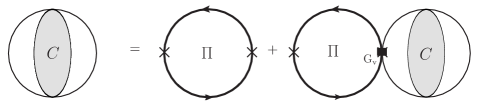
Figure 1: Vector correlator in ring resummation.

We intend here to consider the isoscalar-vector interaction. Generally, from the structure of the interaction one can write the full vector channel correlation function by a geometric progression of one-loop irreducible amplitudes Davidson:1995fq . In the present form of our model Lagrangian with effective coupling $G_{V}$, the Dyson-Schwinger equation (DSE) for the vector correlator $C_{\mu\nu}$ within the ring approximation as shown in Fig. 1 reads as

$$C_{\mu\nu}=\Pi_{\mu\nu}+G_{V}\Pi_{\mu\sigma}C^{\sigma}_{\nu},$$ (19)

where $\Pi_{\mu\nu}$ is one loop vector correlator.

4.1 Ring resummation at zero temperature and chemical potential

The general properties of a vector correlation function at vacuum :

$$\Pi_{\mu\nu}(Q^{2}) = \left(g_{\mu\nu}-\frac{Q_{\mu}Q_{\nu}}{Q^{2}}\right)\Pi(Q^{2}),$$ (20)

$$C_{\mu\nu}(Q^{2}) = \left(g_{\mu\nu}-\frac{Q_{\mu}Q_{\nu}}{Q^{2}}\right)C(Q^{2}),$$ (21)

where $\Pi(Q^{2})$ and $C(Q^{2})$ are scalar quantities with $Q\equiv(q_{0},{\vec{q}})$, is the four momentum.

Using (20) and (21), (19) can be reduced to a scalar DSE as

$$C = \Pi+G_{V}\Pi C$$

$$C = \frac{\Pi}{1-G_{V}\Pi}$$ (22)

The general structure of a vector correlator in vacuum becomes

$$C_{\mu\nu}=\frac{\Pi}{1-G_{V}\Pi}\left(g_{\mu\nu}-\frac{Q_{\mu}Q_{\nu}}{Q^{2}}\right).$$ (23)

Using (23) the spectral representation in vacuum can be obtained from (5). The vacuum properties of vector meson can be studied using this spectral function Davidson:1995fq but we are interested in those at finite temperature and density appropriate for hot and dense medium formed in heavy-ion collisions and the vacuum, as we will see later, is in-built therein. Below we briefly outline how the vector correlation function and its spectral properties will be modified in a hot and dense medium.

4.2 Ring resummation at finite temperature and chemical potential

The general structure of one-loop and resummed vector correlation function in the medium ($T\ {\mbox{and}}\ \mu\neq 0$) can be decomposed Kapusta_Gale(book):1996FTFTPA ; Lebellac(book):1996TFT ; Das(book):FTFT as :

$$\Pi_{\mu\nu}(Q^{2}) = \Pi_{T}(Q^{2})P^{T}_{\mu\nu}+\Pi_{L}(Q^{2})P^{L}_{\mu\nu},$$ (24)

$$C_{\mu\nu}(Q^{2}) = C_{T}(Q^{2})P^{T}_{\mu\nu}+C_{L}(Q^{2})P^{L}_{\mu\nu},$$ (25)

where $\Pi_{L(T)}$ and $C_{L(T)}$ are the respective scalar parts of $\Pi_{\mu\nu}$ and $C_{\mu\nu}$. $P_{\mu\nu}^{L(T)}$ are longitudinal (transverse) projection operators with their well defined properties in the medium and can be chosen as Das(book):FTFT ,

$$P_{\mu\nu}^{L}=\frac{Q^{2}}{\tilde{Q}^{2}}{\bar{U}_{\mu}}{\bar{U}_{\nu}},~{}~{}~{}~{}~{}~{}P_{\mu\nu}^{T}=\eta_{\mu\nu}-U_{\mu}U_{\nu}-\frac{\tilde{Q}_{\mu}\tilde{Q}_{\nu}}{\tilde{Q}^{2}}.$$ (26)

Here $U_{\mu}$ is the proper four velocity which in the rest frame of the heat bath has the form $U_{\mu}=(1,0,0,0)$. $\tilde{Q}_{\mu}=(Q_{\mu}-\omega U_{\mu})$ is the four momentum orthogonal to $U_{\mu}$ whereas $\bar{U}_{\mu}=(U_{\mu}-\omega Q_{\mu}/Q^{2})$ is orthogonal component of $U_{\mu}$’s with respect to the four momentum $Q_{\mu}$. Also, the respective scalar parts, $\Pi_{L(T)}$, of $\Pi_{\mu\nu}$ are obtained as

$$\Pi_{L}=-\frac{Q^{2}}{{q}^{2}}\Pi_{00};~{}~{}~{}~{}~{}~{}~{}\Pi_{T}=\frac{1}{(D-2)}\left[\frac{\omega^{2}}{{q}^{2}}\Pi_{00}-\Pi_{ii}\right],$$ (27)

where $D$, is the space-time dimension of the theory.

Using (24) and (25) in (19) one obtains

$$C_{T}(Q^{2})P^{T}_{\mu\nu}+C_{L}(Q^{2})P^{L}_{\mu\nu} = \left[\Pi_{T}+G_{V}\Pi_{T}C_{T}\right]P^{T}_{\mu\nu}+\left[\Pi_{L}+G_{V}\Pi_{L}C_{L}\right]P^{L}_{\mu\nu}.$$ (28)

Now, the comparison of coefficients on both sides leads to two scalar DSEs: One, for transverse mode, reads as

$$C_{T} = \frac{\Pi_{T}}{1-G_{V}\Pi_{T}},$$ (29)

and the other one, for the longitudinal mode, reads as:

$$C_{L} = \frac{\Pi_{L}}{1-G_{V}\Pi_{L}}$$ (30)

Let us first write the temporal component of the resummed correlator: it is clear from (26) that $P_{00}^{T}=0$. So we have from (25)

$$C_{00} = \frac{\Pi_{L}}{1-G_{V}\Pi_{L}}P_{00}^{L}=\frac{\Pi_{00}}{1+G_{V}\frac{Q^{2}}{{q}^{2}}\Pi_{00}},$$ (31)

and the imaginary part of the temporal component of $C_{00}$ is obtained as

$${\rm ImC_{00}}=\frac{{\rm Im\Pi_{00}}}{\Big{[}1-G_{V}\Big{(}1-\frac{\omega^{2}}{{q}^{2}}\Big{)}{\rm Re\Pi_{00}}\Big{]}^{2}+\Big{[}G_{V}(1-\frac{\omega^{2}}{{q}^{2}}){\rm Im\Pi_{00}}\Big{]}^{2}}.$$ (32)

The spatial component of the resummed correlator ($C_{ii}$) can be written as:

$$C_{ii}=C_{T}P_{ii}^{T}+C_{L}P_{ii}^{L}=\frac{\Pi_{T}}{1-G_{V}\Pi_{T}}P_{ii}^{T}+\frac{\Pi_{L}}{1-G_{V}\Pi_{L}}P_{ii}^{L}.$$ (33)

Using (29) and (30), it becomes for $D=4$

$$C_{ii} = \frac{\Pi_{ii}-\frac{\omega^{2}}{q^{2}}\Pi_{00}}{1-\frac{G_{V}}{2}(\frac{\omega^{2}}{q^{2}}\Pi_{00}-\Pi_{ii})}+\frac{\frac{\omega^{2}}{q^{2}}\Pi_{00}}{1+G_{V}(\frac{Q^{2}}{q^{2}})\Pi_{00}}$$ (34)

$$= C_{T}^{\prime}+C_{L}^{\prime}.$$

The imaginary part of the spatial vector correlator can be obtained as

$${\mbox{Im}}C_{ii}={\mbox{Im}}C_{T}^{\prime}+{\mbox{Im}}C_{L}^{\prime}.$$ (35)

where

$${\rm Im}C_{T}^{\prime}=\frac{{\rm{Im}}\Pi_{ii}-\frac{\omega^{2}}{{q}^{2}}{\rm{Im}}\Pi_{00}}{\left[1+\frac{G_{V}}{2}{\rm{Re}}\Pi_{ii}-\frac{G_{V}}{2}\frac{\omega^{2}}{{q}^{2}}{\rm{Re}}\Pi_{00}\right]^{2}+\frac{G_{V}^{2}}{4}\Big{[}{{\rm{Im}}\Pi_{ii}-\frac{\omega^{2}}{{q}^{2}}\rm{{Im}}\Pi_{00}}\Big{]}^{2}},$$ (36)

and,

$${\rm Im}C_{L}^{\prime}=\frac{\frac{\omega^{2}}{{q}^{2}}\rm{Im}\Pi_{00}}{\Big{[}1-G_{V}\Big{(}1-\frac{\omega^{2}}{{q}^{2}}\Big{)}{\rm Re\Pi_{00}}\Big{]}^{2}+\Big{[}G_{V}(1-\frac{\omega^{2}}{{q}^{2}}){\rm Im\Pi_{00}}\Big{]}^{2}}=\frac{\omega^{2}}{{q}^{2}}{\rm Im}C_{00}.$$ (37)

Folowing (5), the resummed vector spectral function

$$\sigma_{V}=\frac{1}{\pi}\Big{[}{\rm Im}C_{00}-{\rm Im}C_{ii}\Big{]}.$$ (38)

4.3 Conserved Density Fluctuation in Ring Approximation

Following (8) the response to the conserved density fluctuation, i.e., QNS, at finite $T$ and $\mu$ in ring approximation can be obtained in terms of the real part of the temporal correlation function $C_{00}$. The real part of $C_{00}$ is obtained from (31) as

$${\rm{Re}}C_{00}(\omega,\vec{q}) = \frac{{\rm{Re}}\Pi_{00}(\omega,\vec{q})+G_{V}\left(\frac{\omega^{2}}{q^{2}}-1\right)\left[({\rm{Re}}\Pi_{00}(\omega,\vec{q}))^{2}+({\rm{Im}}\Pi_{00}(\omega,\vec{q}))^{2}\right]}{1+2G_{V}{\left(\frac{\omega^{2}}{q^{2}}-1\right){\rm{Re}}\Pi_{00}(\omega,\vec{q})}+\left(G_{V}(\frac{\omega^{2}}{q^{2}}-1)\right)^{2}\Big{[}({\rm{Re}}\Pi_{00}(\omega,\vec{q}))^{2}+({\rm{Im}}\Pi_{00}(\omega,\vec{q}))^{2}\Big{]}}.$$

Now the resummed QNS in ring approximation becomes

$$\chi^{R}_{q}(T,\tilde{\mu})=-\lim_{\vec{q}\rightarrow 0}{\rm{Re}}C_{00}(0,\vec{q})=\frac{\chi_{q}(T,\tilde{\mu})}{1+G_{V}\chi_{q}(T,\tilde{\mu})},$$ (40)

where we note that $\lim_{{\vec{q}}\rightarrow 0}{\rm{Im}}\Pi_{00}(0,\vec{q})=0$ and one-loop $\chi_{q}(T,\tilde{\mu})=-\lim_{\vec{q}\rightarrow 0}{\rm{Re}}\Pi_{00}(0,\vec{q})$.

Now, we note that at $G_{V}=0$, all the resummed quantities in ring approximation become equivalent to those of one-loop. To compute all resummed quantities, we just need to compute one-loop vector self-energy within the effective models considered here.

4.4 Vector correlation function in one-loop

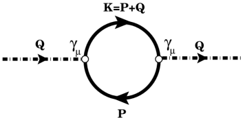
Figure 2: Vector channel correlator at one-loop.

The current-current correlator in vector channel at one-loop level can be written as

$$\Pi_{\mu\nu}(Q)=\int\frac{d^{4}P}{(2\pi)^{4}}{\rm{Tr}}_{D,c}\left[\gamma_{\mu}S(P+Q)\gamma_{\nu}S(P)\right],$$ (41)

where ${\textrm{Tr}}_{D,c}$ is trace over Dirac and color indices, respectively. We would like to compute this in effective models, viz., in NJL and PNJL model.

The NJL quark propagator in Hartree approximation is given as

$${S_{\textrm{NJL}}}(L)=\left[\not{l}-m_{0}+\gamma_{0}\tilde{\mu}+G_{S}\sigma\right]^{-1}=\left[\not{l}-M_{f}+\gamma_{0}{\tilde{\mu}}\right]^{-1},$$ (42)

whereas for PNJL it reads as

$$S_{\textrm{PNJL}}(L)=\left[\not{l}-M_{f}+\gamma_{0}{\tilde{\mu}}-i\gamma_{0}{\cal A}_{4}\right]^{-1}$$ (43)

where the four momentum, $L\equiv(l_{0},{\vec{l}}\hskip 1.42271pt)$. The gap equation for constituent quark mass $M_{f}$ and the modified quark chemical potential $\tilde{\mu}$ due to vector coupling $G_{V}$ are given, respectively, in (13) and (14). Now in contrast to NJL one, the presence of background temporal gauge field ${\cal A}_{4}$ will make a connection to the Polyakov Loop field $\Phi$ Pisarski:2000eq ; Dumitru:2001xa ; Dumitru:2002cf ; Dumitru:2003hp ; Gross:1980br ; Gocksch:1993iy ; Weiss:1980rj ; Weiss:1981ev . While performing the frequency sum and color trace in (41), the thermal distribution function in PNJL case will be different from that of NJL one.

For convenience, we will calculate the one-loop vector correlation in NJL model. This NJL correlation function, as discussed, can easily be generalized to PNJL one by replacing the thermal distribution function  as

$$f(E_{p}\pm\tilde{\mu})=\frac{\Phi e^{-\beta(E_{p}\pm\tilde{\mu})}+2\bar{\Phi}e^{-2\beta(E_{p}\pm\tilde{\mu})}+e^{-3\beta(E_{p}\pm\tilde{\mu})}}{1+3\Phi e^{-\beta(E_{p}\pm\tilde{\mu})}+3\bar{\Phi}e^{-2\beta(E_{p}\pm\tilde{\mu})}+e^{-3\beta(E_{p}\pm\tilde{\mu})}},$$ (44)

which at $\Phi({\bar{\Phi}})=1$ reduces to the thermal distribution for NJL or free as the cases may be. On the other hand for $\Phi({\bar{\Phi}})=0$, the effect of confinement is clearly evident in which three quarks are stacked in a same momentum and color state Islam:2014tea .

4.4.1 Temporal Part

The time-time component of the vector correlator in (41) reads as

$$\Pi_{00}(Q)=\int{\frac{d^{4}P}{(2\pi)^{4}}{\mathrm{Tr}}[\gamma_{0}S(K)\gamma_{0}S(P)]},$$ (45)

where $K=P+Q$. After some mathematical simplifications we are left with

$$\Pi_{00}(\omega,\vec{q}) = N_{c}N_{f}\int\frac{d^{3}p}{(2\pi)^{3}}\frac{1}{E_{p}E_{k}}\Bigg{\{}\frac{E_{p}E_{k}+M_{f}^{2}+\vec{p}\cdot\vec{k}}{\omega+E_{p}-E_{k}}$$ (46)

$$\times\left[f(E_{p}-\tilde{\mu})+f(E_{p}+\tilde{\mu})-f(E_{k}-\tilde{\mu})-f(E_{k}+\tilde{\mu})\right]$$

$$+\left(E_{p}E_{k}-M_{f}^{2}-\vec{p}\cdot\vec{k}\right)\left[\frac{1}{\omega-E_{p}-E_{k}}-\frac{1}{\omega+E_{p}+E_{k}}\right]$$

$$\times\left[1-f(E_{p}+\tilde{\mu})-f(E_{k}-\tilde{\mu})\right]\Bigg{\}}.$$

The real and imaginary parts of the temporal vector correlator are, respectively, obtained as

$$\textrm{Re}\Pi_{00}(\omega,\vec{q}) = {\large{\textrm{P}}}\Bigg{[}\ N_{f}N_{c}\int\frac{d^{3}p}{(2\pi)^{3}}\frac{1}{E_{p}E_{k}}\Bigg{\{}\frac{E_{p}E_{k}+M_{f}^{2}+\vec{p}\cdot\vec{k}}{\omega+E_{p}-E_{k}}$$ (47)

$$\times\left[f(E_{p}-\tilde{\mu})+f(E_{p}+\tilde{\mu})-f(E_{k}-\tilde{\mu})-f(E_{k}+\tilde{\mu})\right]$$

$$+(E_{p}E_{k}-M_{f}^{2}-\vec{p}\cdot\vec{k})\left(\frac{1}{\omega-E_{p}-E_{k}}-\frac{1}{\omega+E_{p}+E_{k}}\right)$$

$$\times\left[1-f(E_{p}+\tilde{\mu})-f(E_{k}-\tilde{\mu})\right]\Bigg{\}}\Bigg{]},$$

as P stands for principal value, and

$${\textrm{Im}}\Pi_{00}(\omega,\vec{q}) = \lim_{\eta\rightarrow 0}\ \frac{1}{2i}\Big{[}\Pi_{00}(\omega\rightarrow\omega+i\eta,q)-\Pi_{00}(\omega\rightarrow\omega-i\eta,q)\Big{]}$$ (48)

$$= -\pi N_{f}N_{c}\int\frac{d^{3}p}{(2\pi)^{3}}\frac{1}{E_{p}E_{k}}\Bigg{\{}(E_{p}E_{k}+M_{f}^{2}+\vec{p}\cdot\vec{k})$$

$$\times\left[f(E_{p}-\tilde{\mu})+f(E_{p}+\tilde{\mu})-f(E_{k}-\tilde{\mu})-f(E_{k}+\tilde{\mu})\right]\times\delta(\omega+E_{p}-E_{k})$$

$$+(E_{p}E_{k}-M_{f}^{2}-\vec{p}\cdot\vec{k})\left[1-f(E_{p}+\tilde{\mu})-f(E_{k}-\tilde{\mu})\right]$$

$$\times[\delta(\omega-E_{p}-E_{k})]\Bigg{\}}.$$

It is now worthwhile to check some known results in the limit $\vec{q}\rightarrow 0$ and $\tilde{\mu}=0$, (48) can be written as:

$$\textrm{Im}\Pi_{00}(\omega) = -\pi N_{f}N_{c}\int\frac{d^{3}p}{(2\pi)^{3}}\frac{1}{E_{p}^{2}}\left(3E_{p}^{2}-3M_{f}^{2}-p^{2}\right)\left(2f^{\prime}(E_{p})\right)\left(-\omega\delta\left(\omega\right)\right),$$ (49)

and which, in the limit $M_{f}=m_{0}-G_{S}\sigma=0$, further becomes

$$\textrm{Im}\Pi_{00}(\omega) = -2\pi T^{2}\omega\delta(\omega).$$ (50)

The vacuum part in (47) is now separated as

$${\textrm{Re}}\Pi_{00}^{\textrm{vac}}(\omega,\vec{q})\!\! = \!\!\frac{N_{f}N_{c}}{4\pi^{2}}\!\!\int_{0}^{\Lambda}\!\!p\ dp\frac{1}{2E_{p}q}\left[4pq+6E_{p}X_{-}-6E_{p}X_{+}-Y_{-}\ln\left|\frac{E_{p}+X_{-}-\omega}{E_{p}+X_{+}-\omega}\right|\right.$$ (51)

$$\left.+Y_{+}\ln\frac{E_{p}+X_{+}+\omega}{E_{p}+X_{-}+\omega}\right],$$

$${\textrm{with}}\,\,\,\,Y_{\pm} = (4E_{p}^{2}\pm 4E_{p}\omega+M^{2}),\,\,\,\,X_{\pm}=\sqrt{E_{p}^{2}\pm 2pq+q^{2}}\ \ \ {\textrm{and}}\ \ \ \ M^{2}=\omega^{2}-q^{2}.$$ (52)

We note that the ultraviolet divergence in the vacuum part is regulated by using a finite three momentum cut-off $\Lambda$. The corresponding matter part of (47) is obtained as

$${\textrm{Re}}\Pi_{00}^{\textrm{mat}}(\omega,\vec{q}) = \frac{N_{f}N_{c}}{2\pi^{2}}\int_{0}^{\infty}p\ dp\big{[}f(E_{p}-\tilde{\mu})+f(E_{p}+\tilde{\mu})\big{]}\left[\frac{\omega}{q}\ln\left|\frac{M^{2}-4\left(pq+\omega E_{p}\right)^{2}}{M^{2}-4\left(pq-\omega E_{p}\right)^{2}}\right|\right.$$ (53)

$$\left.-\left(\frac{4E_{p}^{2}+M^{2}}{4qE_{p}}\right)\ln\left|\frac{\left(M^{2}-2pq\right)^{2}-4\omega^{2}E_{p}^{2}}{\left(M^{2}+2pq\right)^{2}-4\omega^{2}E_{p}^{2}}\right|-\frac{2p}{E_{p}}\right].$$

The imaginary part in (48) can be simplified as

$${\textrm{Im}}\Pi_{00}(\omega,\vec{q}) = \frac{N_{f}N_{c}}{4\pi}\!\!\!\int_{p_{-}}^{p_{+}}\!\!\!p\ dp\ \frac{4\omega E_{p}-4E_{p}^{2}-M^{2}}{2E_{p}q}\ \big{[}f(E_{p}-\tilde{\mu})+f(E_{p}+\tilde{\mu})-1\big{]}$$ (54)

where the vacuum part does not require any momentum cut-off as the energy conserving $\delta$-function ensures the finiteness of the limits:

$$p_{\pm}={\frac{\omega}{2}\sqrt{1-\frac{4M_{f}^{2}}{M^{2}}}\pm\frac{q}{2}},$$ (55)

with a threshold restricted by a step function, $\Theta(M^{2}-4M_{f}^{2})$.

4.4.2 Spatial Part

The space-space component of the vector correlator in (41) reads as

$$\Pi_{ii}(Q)=\int{\frac{d^{4}P}{(2\pi)^{4}}{\mathrm{Tr}}[\gamma_{i}S(K)\gamma_{i}S(P)]},$$ (56)

which can be simplified to

$$\Pi_{ii}(\omega,\vec{q}) = N_{c}N_{f}\int\frac{d^{3}p}{(2\pi)^{3}}\frac{1}{E_{p}E_{k}}\Bigg{\{}\frac{3E_{p}E_{k}-3M_{f}^{2}-\vec{p}\cdot\vec{k}}{\omega-E_{p}+E_{k}}$$ (57)

$$\times\left[f(E_{k}+\tilde{\mu})+f(E_{k}-\tilde{\mu})-f(E_{p}+\tilde{\mu})-f(E_{p}-\tilde{\mu})\right]$$

$$+\left(3E_{p}E_{k}+3M_{f}^{2}+\vec{p}\cdot\vec{k}\right)\left[\frac{1}{\omega-E_{p}-E_{k}}-\frac{1}{\omega+E_{p}+E_{k}}\right]$$

$$\times\left[1-f(E_{k}+\tilde{\mu})-f(E_{p}-\tilde{\mu})\right]\Bigg{\}}.$$

In the similar way as before the imaginary part can be obtained

$${\textrm{Im}}\Pi_{ii}(\omega,\vec{q}) = -\pi N_{f}N_{c}\int\frac{d^{3}p}{(2\pi)^{3}}\frac{1}{E_{p}E_{k}}\Bigg{\{}(3E_{p}E_{k}-3M_{f}^{2}-\vec{p}\cdot\vec{k})$$ (58)

$$\times\left[f(E_{k}+\tilde{\mu})+f(E_{k}-\tilde{\mu})-f(E_{p}+\tilde{\mu})-f(E_{p}-\tilde{\mu})\right]\delta(\omega+E_{p}-E_{k})$$

$$+\left(3E_{p}E_{k}+3M_{f}^{2}+\vec{p}\cdot\vec{k}\right)\left[1-f(E_{k}+\tilde{\mu})-f(E_{p}-\tilde{\mu})\right]$$

$$\times\delta(\omega-E_{p}-E_{k})\Bigg{\}},$$

whereas the real part can be obtained as

$$\textrm{Re}\Pi_{ii}(\omega,\vec{q}) = {\large{\textrm{P}}}\Bigg{[}N_{f}N_{c}\int\frac{d^{3}p}{(2\pi)^{3}}\frac{1}{E_{p}E_{k}}\Bigg{\{}\frac{3E_{p}E_{k}-3M_{f}^{2}-\vec{p}\cdot\vec{k}}{\omega-E_{p}+E_{k}}$$ (59)

$$\times\left[f(E_{k}-\tilde{\mu})+f(E_{k}+\tilde{\mu})-f(E_{p}-\tilde{\mu})-f(E_{p}+\tilde{\mu})\right]$$

$$+(3E_{p}E_{k}+3M_{f}^{2}+\vec{p}\cdot\vec{k})\left(\frac{1}{\omega-E_{p}-E_{k}}-\frac{1}{\omega+E_{p}+E_{k}}\right)$$

$$\times\left[1-f(E_{k}+\tilde{\mu})-f(E_{p}-\tilde{\mu})\right]\Bigg{\}}\Bigg{]}.$$

At this point we also check the known results in the limit $\vec{q}\rightarrow 0$ and $\tilde{\mu}=0$, (58) can be written as:

$$\textrm{Im}\Pi_{ii}(\omega) = -\pi N_{f}N_{c}\int\frac{d^{3}p}{(2\pi)^{3}}\frac{1}{E_{p}^{2}}\left(3E_{p}^{2}-3M_{f}^{2}-p^{2}\right)\left(2f^{\prime}(E_{p})\right)\left(-\omega\delta\left(\omega\right)\right)$$ (60)

$$-\frac{3}{2\pi\omega}\sqrt{\omega^{2}-4M_{f}^{2}}\left(\omega^{2}+2M_{f}^{2}\right)\tanh\left(\frac{\omega}{4T}\right)\Theta(\omega-2M_{f}),$$

and when $M_{f}=m_{0}-G_{S}\sigma=0$, it becomes

$$\textrm{Im}\Pi_{ii}(\omega) = -2\pi T^{2}\omega\delta(\omega)-{\frac{3}{2\pi}}\omega^{2}\tanh\left(\frac{\omega}{4T}\right).$$ (61)

As seen both massive and massless cases show a sharp peak due to the delta function at $\omega\rightarrow 0$, which leads to pinch singularity for calculation of transport coefficients.

Now, the vacuum part in (59) is simplified as

$${\textrm{Re}}\Pi^{\textrm{vac}}_{ii}(\omega,\vec{q})\!\!\! = \!\!\!\frac{N_{f}N_{c}}{4\pi^{2}}\!\!\int_{0}^{\Lambda}\!\!\!\!p\ dp\ \frac{1}{2E_{p}q}\left[-4pq+10E_{p}(X_{-}-X_{+})-Z_{-}\ln\left|\frac{E_{p}+X_{-}-\omega}{E_{p}+X_{+}-\omega}\right|\right.$$ (62)

$$\left.+Z_{+}\ln\frac{E_{p}+X_{+}+\omega}{E_{p}+X_{-}+\omega}\right],$$

where $Z_{\pm}=4p^{2}\pm 4E_{p}\omega-M^{2}$. The corresponding matter part is obtained as

$${\textrm{Re}}\Pi_{ii}^{\textrm{mat}}(\omega,\vec{q}) = \frac{N_{f}N_{c}}{4\pi^{2}}\int_{0}^{\infty}p\ dp\ \big{[}f(E_{p}-\tilde{\mu})+f(E_{p}+\tilde{\mu})\big{]}\left[2\frac{\omega}{q}\ln\left|\frac{M^{2}-4(pq+E_{p}\omega)^{2}}{M^{2}-4(pq-E_{p}\omega)^{2}}\right|\right.$$ (63)

$$\left.+\left(\frac{M^{2}-4p^{2}}{2qE_{p}}\right)\ln\left|\frac{\left(M^{2}-2pq\right)^{2}-4\omega^{2}E_{p}^{2}}{\left(M^{2}+2pq\right)^{2}-4\omega^{2}E_{p}^{2}}\right|+4\frac{p}{E_{p}}\right].$$

Finally, the imaginary part in (58) is simplified as

$${\textrm{Im}}\Pi_{ii}(\omega,\vec{q}) = \frac{N_{f}N_{c}}{4\pi}\int_{p_{-}}^{p_{+}}p\ dp\ \frac{4\omega E_{p}-4p^{2}+M^{2}}{2E_{p}q}\ \left(f(E_{p}-\tilde{\mu})+f(E_{p}+\tilde{\mu})-1\right)$$ (64)

where the vacuum part does not need any finite momentum cut-off as stated above.

5 Results

5.1 Gap Equations and Mean Fields

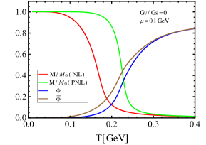
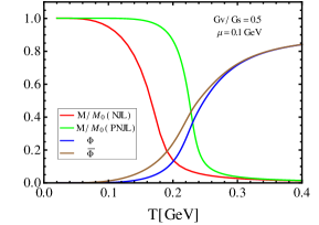
Figure 3: Variation of scaled constituent quark mass with zero temperature quark mass and the Polyakov Loop fields ($\Phi$ and $\bar{\Phi}$) with temperature at chemical potential $\mu=100$ MeV for (a) $G_{V}/G_{S}=0$ and (b) $G_{V}/G_{S}=0.5$.

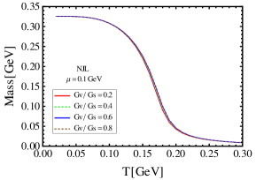
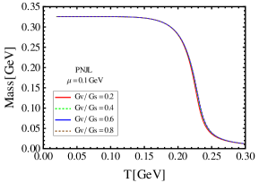
Figure 4: Variation of constituent quark mass with temperature in (a) NJL and (b) PNJL model for chemical potential $\mu=100$ MeV and a set of values for vector coupling $G_{V}$.

The thermodynamic potential $\Omega$ for both NJL and PNJL model is extremized with respect to the mean fields X, i.e.,

$$\frac{\partial\Omega}{\partial X}=0$$ (65)

where, X stands for $\sigma$ and $n$ for NJL model and $\Phi,\bar{\Phi},\sigma$ and $n$ for PNJL model. The value of the parameters, $G_{S}=10.08\ {\textrm{GeV}}^{-2}$ and $\Lambda=0.651$ GeV were taken from literature Ratti:2005jh and $m_{0}=0.005$ GeV. However, the value of $G_{V}$ is difficult to fix within the model formalism, since this quantity should be fixed using the $\rho$ meson mass which, in general, happens to be higher than the maximum energy scale $\Lambda$ of the model. So, we consider the vector coupling constant $G_{V}$ as a free parameter and different choices are considered as ${G_{V}}=x\times{G_{S}}$, where $x$ is chosen from $0$ to $1$ appropriately.

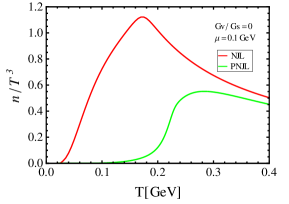
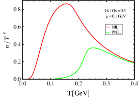
Figure 5: Comparison of the scaled quark number density with $T^{3}$ as a function of $T$ in NJL and PNJL model with chemical potential $\mu=100$ MeV for (a) $G_{V}/G_{S}=0$ and (b) $G_{V}/G_{S}=0.5$ .

In Fig. 3 a comparison between the scaled quark mass with its zero temperature value ($M_{f}(T)/M_{f}(0)$) in NJL and PNJL model is displayed as a function of temperature $T$ for two values of $G_{V}(=0\ {\textrm{and}}\ 0.5G_{S})$ with $\mu=100$MeV. It also contains a variation of the Polyakov loop fields ($\Phi(T)$ and $\bar{\Phi}(T)$) with $T$. In both models the scaled quark mass decreases with increase in $T$ and approaches the chiral limit at very high $T$. However, in the temperature range $60\leq T({\textrm{MeV}})\leq 300$, the variation of the scaled quark mass is slower in PNJL than that of NJL model. This slow variation is due to the presence of the confinement effect in it through the Polyakov Loop fields ($\Phi(T)$ and $\bar{\Phi}(T)$), as can be seen that the Polyakov Loop field ($\Phi(T)$) and its conjugate ($\bar{\Phi}(T)$) increase from zero in confined phase and approaches unity (free state) at high temperature. Now, we note that $\Phi={\bar{\Phi}}$ at $\mu=0$ as there is equal number of quarks and antiquarks. However, because of non-zero chemical potential there is an asymmetry in quark and antiquark numbers, which leads to an asymmetry in the Polyakov Loop fields $\Phi$ and $\bar{\Phi}$. This asymmetry disappears for $T>300$ MeV, which is much greater than $\mu$. We also note that the fields depend weakly with the variation of the vector coupling $G_{V}$ akin to that of mass as displayed in Fig. 4 for $\mu=100$ MeV and $G_{V}/G_{S}=0\ {\textrm{to}}\ 0.8$.

In Fig. 5 the number density scaled with $T^{3}$ for both NJL and PNJL model is displayed as a function of $T$ with $\mu=100$ MeV for two values of $G_{V}$. At very high temperature, as seen in Fig. 3, the Polyakov Loop fields $\Phi({\bar{\Phi}})\rightarrow 1$ and masses in both models become same. So, PNJL model becomes equivalent to NJL model because the thermal distribution function becomes equal as can be seen from (44) and thus the number density. On the other hand, for temperature $T<400$ MeV and a given $\mu$, the PNJL number density is found to be suppressed than that of NJL case as the thermal distribution function in (44) is suppressed. This is due to the combination of two complementary effects: (i) the nonperturbative effect through $\Phi$ and ${\bar{\Phi}}$ and (ii) the slower variation of mass in PNJL model, which are clearly evident from Fig. 3. It is also obvious from Fig. 5 and Fig. 5 that the presence of vector interaction $G_{V}$ reduces the number density for both NJL and PNJL model, which could be understood due to the reduction of ${\tilde{\mu}}$ as given in (14).

5.2 Vector spectral function and dilepton rate

The vector spectral function is proportional to the imaginary part of the vector correlation function as defined in (5) or (38). This imaginary part is restricted by, the energy conservation, $\omega=E_{p}+E_{k}$, as can be seen from (48) and (58). This equivalently leads to a threshold, $M^{2}\geq 4M_{f}^{2}$, which can also be found from (55). Now for a given $G_{V}$ and $T$, the resummed spectral function in (38) picks up continuous contribution above the threshold, $M^{2}>4M^{2}_{f}$, which provides a finite width to a vector meson that decays into a pair of leptons. However, below the threshold $M^{2}<4M^{2}_{f}$, the continuous contribution of the spectral function in (38) becomes zero and the decay to dileptons are forbidden. But if one analyses it below the threshold, one can find bound state contributions in spectral functions. When imaginary part approaches zero, the spectral function in (38) becomes discrete and can be written as:

$$\sigma_{V}(\omega,\vec{q}) =\atop{M<2M_{f}} \frac{1}{\pi}\Big{[}\delta\big{(}F_{1}(\omega,\vec{q})\big{)}\Big{]},$$

$$\textrm{where}\,\,\,\,\,\,\,\,\,F_{1}(\omega,\vec{q}) = {1+\frac{G_{V}}{2}{\rm{Re}}\Pi_{ii}-\frac{G_{V}}{2}\frac{\omega^{2}}{{q}^{2}}{\rm{Re}}\Pi_{00}}=0,$$ (66)

where only the dominant contribution of (36) is considered. Using the properties of $\delta$-function, one can write

$$\sigma_{V}(\omega,\vec{q}) =\atop{M<2M_{f}} \frac{1}{\pi}\frac{\delta(\omega-\omega_{0})}{\left|dF_{1}(\omega,\vec{q})/d\omega\right|_{\omega=\omega_{0}}},$$ (67)

which corresponds to a sharp $\delta$-function peak at $\omega=\omega_{0}$. However, we are interested here in continuous contribution $M>2M_{f}$, which are discussed below.

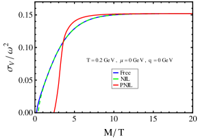
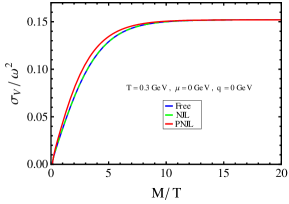
Figure 6: Scaled vector spectral function $\sigma_{V}/\omega^{2}$ as a function of scaled invariant mass, $M/T$, in NJL and PNJL model with external momentum $q=0$, quark chemical potential $\mu=0$ and $G_{V}/G_{S}=0$ for (a) $T=200$ MeV and (b) $T=300$ MeV

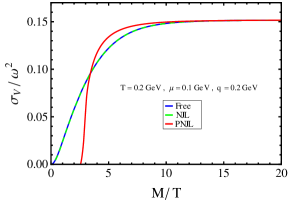
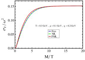
Figure 7: Scaled vector spectral function $\sigma_{V}/\omega^{2}$ as a function of scaled invariant mass, $M/T$, in NJL and PNJL model with external momentum $q=200$ MeV, quark chemical potential $\mu=100$ MeV and $G_{V}/G_{S}=0$ for (a) $T=200$ MeV and (b) $T=300$ MeV

5.2.1 Without vector interaction ($G_{V}=0$)

With no vector interaction ($G_{V}=0$), the spectral function in (38) is solely determined by the imaginary part of the one loop vector self energies $\Pi_{00}(\omega,\vec{q})$ and $\Pi_{ii}(\omega,\vec{q})$. Fig. 6 displays a comparison of vector spectral function with zero external momentum ($\vec{q}=0,\ \ M=\omega$) in NJL and PNJL model for $T=200$ MeV and $300$ MeV, when there is no vector interaction ($G_{V}=0$). Now, for $T=200$ MeV (left panel) the spectral function in PNJL model has larger threshold than NJL model because the quark mass in PNJL model is much larger than that of NJL one (see Fig. 3). Also the PNJL spectral function dominates over that of NJL one, because of the presence of nonperturbative effects due to Polyakov Loop fields $\Phi$ and ${\bar{\Phi}}$. At higher values of $T~{}(=300~{}\rm{MeV})$ (right panel), the threshold becomes almost same due to the reduction of mass effect in PNJL case whereas the nonperturbative effects at low $M/T$ still dominate. The reason is the following: at zero external momentum and zero chemical potential the spectral function is proportional to $[1-2f(E_{p})]$ (apart from the mass dependent prefactor) as can be seen from the second term of (60). In PNJL case the thermal distribution function, $f(E_{p})$, is more suppressed due to the suppression of color degrees of freedom than NJL at moderate values of $T$, so the weight factor $[1-2f(E_{p})]$ is larger than NJL case and causing an enhancement in the spectral function . All these features also persist at non-zero chemical potential and external momentum as can also be seen from Fig. 7.

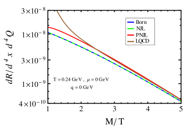
Figure 8: Comparison of dilepton rates as a function of $M/T$ for $T=240$ MeV with external momentum $q=0$, quark chemical potential $\mu=0$ and $G_{V}/G_{S}=0$. The LQCD rate is from Ref. Ding:2010ga .

At this point it is important to note that for $T>250$ MeV the mass in NJL model almost approaches current quark mass (see Fig. 3) and can be considered as a free case since there is no vector interaction present ($G_{V}=0$). Nevertheless, the PNJL case is different because of the presence of the nonperturbative confinement effect through the Polyakov Loop fields. The PNJL model can suitably describe a semi-QGP Fukushima:2003fw ; Fukushima:2003fm ; Gale:2014dfa scenario having nonperturbative effect due to the suppression of color degrees of freedom compared to NJL vis-a-vis free case above the deconfinement temperature.

The above features of the spectral function in a semi-QGP with no vector interaction will be reflected in the dilepton rate which is related to the spectral function, as given in (7). In Fig. 8, the dilepton rate is displayed as a function of scaled invariant mass $M$ with $T$. As already discussed, at this temperatures the quark mass in NJL approaches current quark mass faster than PNJL, thus the dilepton rates for Born and NJL cases become almost the same. However, the dilepton rate in PNJL model is enhanced than those of Born or NJL case. This in turn suggests that the nonperturbative dilepton production rate is higher in a semi-QGP than the Born rate in a weakly coupled QGP. The dilepton rate is also compared with that from LQCD result Ding:2010ga within a quenched approximation. It is found to agree well for $M/T\geq 2$, below which it differs from LQCD rate. We try to understand this as follows: the spectral function in LQCD is extracted using MEM from Euclidean vector correlation function by inverting (6), which requires an ansatz for the spectral function. Using a free field spectral function as an ansatz, the spectral function in a quenched approximation of QCD was obtained earlier Karsch:2001uw by inverting (6), which was then approaching zero in the limit $M/T\rightarrow 0$. So was the first lattice dilepton rate Karsch:2001uw at low $M/T$ whereas it was oscillating around the Born rate for $M/T>3$. Now, in a very recent LQCD calculation Ding:2010ga with larger size, while extracting the spectral function using MEM from Euclidean vector correlation function, an ansatz for the spectral function, a Briet-Wigner (BW) for low $M/T$ plus a free field one for $M/T\geq 2$, has been used. The ansatz of BW at low $M/T$ pushes up the spectral function and so is the recent dilepton rate in LQCD below $M/T\leq 2$. However, no such ansatz is required in thermal QCD and we can directly calculate the spectral function without any uncertainty by virtue of the analytic continuation.

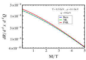
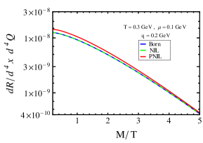
Figure 9: Different dilepton rates as a function of $M/T$ at $T=300$ MeV, $\mu=100$ MeV and $G_{V}/G_{S}=0$ for (a) $q=0$ (b) $q=200$ MeV

In Fig. 9 the dilepton rate is also displayed at $T=300$ MeV, non-zero chemical potential ($\mu=100$ MeV) and external momentum ($q=0$ and $200$ MeV). We note that this information could also be indicative for future LQCD computation of dilepton rate at non-zero $\mu$ and $q$. The similar feature of semi-QGP as found in Fig. 8 is also seen here but with a quantitative difference especially due to higher $T$, which could be understood from Fig. 3.

5.2.2 With vector interaction ($G_{V}\neq 0$)

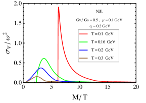
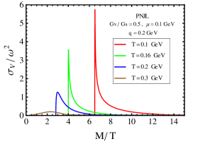
Figure 10: Scaled spectral function as a function of $M/T$ in (a) NJL and (b) PNJL model for a set of $T$ with $\mu=100$ MeV, $q=200$ MeV and $G_{V}/G_{S}=0.5$. Note the difference in $y$-scale.

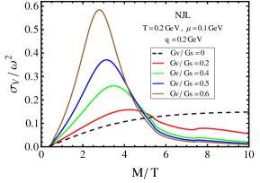
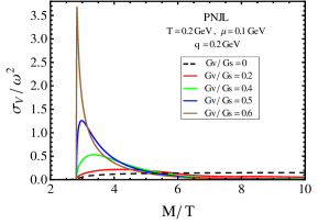
Figure 11: Scaled spectral function as a function of $M/T$ for (a) NJL and (b) PNJL model with $T=200$ MeV, $\mu=100$ MeV, $q=200$ MeV and a set of values of $G_{V}/G_{S}=0,\,0.2,\,0.4,\,0.5\,\,{\textrm{and}}\,\,0.6$.

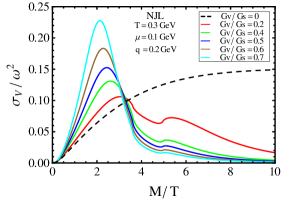
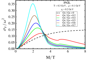
Figure 12: Scaled spectral function as a function of $M/T$ for (a) NJL and (b) PNJL model with $T=300$ MeV, $\mu=100$ MeV, $q=200$ MeV and a set of values of $G_{V}/G_{S}=0,\ 0.2,\,0.4,\,0.5,\,0.6\,\,{\textrm{and}}\,\,0.7$.

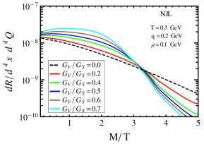
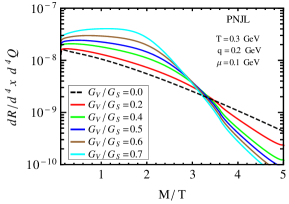
Figure 13: Dilepton rates as a function of $M/T$ (a) NJL and (b) PNJL model for a set of values of $G_{V}/G_{S}$ with $T=300$ MeV with external momentum $q=200$ MeV, quark chemical potential $\mu=100$ MeV.

In Fig. 10 the spectral function for $G_{V}/G_{S}=0.5$ with $q=200$ MeV and $\mu=100$ MeV in NJL (left panel) and PNJL (right panel) model is displayed. At $T=100<T_{c}\sim 160$ MeV Islam:2014tea ; Bazavov:2011nk ; Petreczky:2012ct ; Borsanyi:2010bp the spectral function above the respective threshold, $M>2M_{f}$, starts with a large value because the denominator in (36) is very small compared to those in (32) and (37). This is due to the two reasons: (i) the first term in the denominator involving real parts of $\Pi$ has zero below the threshold that corresponds to a sharp $\delta$-like peak as discussed in (67), thus it also becomes a very small number just above the threshold and (ii) the second term involving imaginary parts start building up, which is also very small. However, the increase in $T$ causes the spectral function to decrease due to mutual effects of denominator (involving both real and imaginary parts of $\Pi$) and numerator (involving only imaginary parts of $\Pi$). On the other hand, with the increase in $T$, the threshold in NJL case reduces quickly as the quark mass decreases faster whereas it reduces slowly for PNJL case because the Polyakov Loop fields experience a slow variation of the quark mass. So, the vector meson in NJL model acquires a width earlier than the PNJL model due to suppression of color degrees of freedom in presence of Polyakov Loop fields. As seen, for NJL model at $T=T_{c}\sim 160$ MeV the sharp peak like structure gets a substantial width than PNJL model. This suggests that the vector meson retains its bound properties at and above $T_{c}$ in PNJL model in presence of $G_{V}$ along with the nonperturbative effects through Polyakov Loop fields.

In Figs. 11 and 12 we present the dependence of the spectral function on the vector interaction in QGP for a set of values of the coupling $G_{V}$ in NJL (left panel) and PNJL (right panel) model, respectively, for $T=200$ and $T=300$ MeV. In both cases the spectral strength increases with that of $G_{V}$. Nevertheless, the strength of the spectral function in PNJL case at a given $T$ and $G_{V}$ is always stronger than that of NJL model. This suggests that the presence of the vector interaction further suppresses the color degrees of freedom in addition to the Polyakov Loop fields. The dilepton rates corresponding to $T=300$ MeV are also displayed in Fig. 13, which show an enhancement at low $M/T$ compared to $G_{V}=0$ case. The enhancement in PNJL case indicates that more lepton pairs will be produced at low mass ($M/T<4$) in semi-QGP with vector interaction, which would be appropriate for the hot and dense matter likely to be produced at FAIR energies.

5.3 Vector Correlation function

The vector correlation function can be obtained using (6) in the scaled Euclidean time $\tau T\in[0,1]$. We note that the correlation function in the $\tau T$ range is symmetrical around $\tau T=1/2$ due to the periodicity condition in Euclidean time guaranteed by the kernel $\cosh[\omega(2\tau T-1)/2T]/\sinh(\omega/2T)$ in (6).

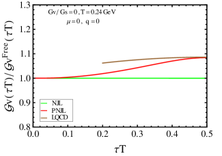
Figure 14: Comparison of various scaled Euclidean correlation function with respect to that of free field theory, ${\cal G}_{V}(\tau T)/{\cal G}_{V}^{\textrm{free}}(\tau T)$, as a function of the scaled Euclidean time $\tau T$ for $T=240$ MeV with external momentum $q=0$, quark chemical potential $\mu=0$ and $G_{V}/G_{S}=0$. The continuum extrapolated LQCD result is from Ref. Ding:2010ga .

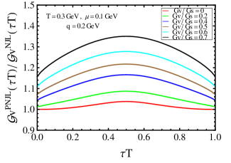
Figure 15: Ratio of Euclidean correlation function in PNJL model to that of NJL model as a function of $\tau T$ at $T=300$ MeV, $\mu=100$ MeV and $q=200$ MeV with a set of values of $G_{V}/G_{S}$.

In Fig. 14 a comparison of the ratio of the vector correlation function to that of free one is displayed at $T=240$ MeV, $G_{V}/G_{S}=0$, $\mu=0$ and $q=0$ for NJL, PNJL and the continuum extrapolated LQCD data Ding:2010ga in quenched approximation. It is plotted in the $\tau T$ range $[0,1/2]$ because LQCD data are available for the same range. As seen the NJL case becomes equal to that of free one as there is no effects from background gauge fields. On the other hand the PNJL result at $\tau T=0$ and $1$ becomes similar to those of free case because $\sigma_{V}^{\textrm{PNJL}}(\omega)/\sigma_{V}^{\textrm{free}}(\omega)=1$ as $\omega\rightarrow\infty$. Around $\tau T=1/2$ it deviates maximum from the free case due to the difference in spectral function at small $\omega$ and thus a nontrivial correlation exists among color charges due to the presence of the nonperturbative Polyakov Loop fields. This features are consistent with those in the spectral function in Fig. 6 and the dilepton rate in Fig. 8. In contrary, the correlation function around $\tau T=1/2$ agrees better with that of LQCD in quenched approximation Ding:2010ga .

In Fig. 15, we display the effect of the vector interaction $G_{V}$ in addition to the presence of the Polyakov Loop fields in QGP through the ratio of the correlation function in PNJL model to that of NJL model. Here we have displayed the result in the full range of the scaled Euclidean time $\tau T\in[0,1]$. As discussed the ratio is symmetric around $\tau T=1/2$ and always stay above unity. The ratio increases with the increase of the strength of the vector interaction. This is due to the fact that PNJL correlation function is always larger than that of the NJL case since $\sigma_{V}^{\textrm{PNJL}}(\omega,\vec{q})/\sigma_{V}^{\textrm{NJL}}(\omega,\vec{q})>1$, and it is even stronger in particular at small $\omega$ (see Fig. 12). This indicates that the color charges maintain a strong correlation among them due to the presence of both Polyakov Loop fields and the vector interaction. Thus the vector meson retains its bound properties in the deconfined phase.

5.4 Quark number susceptibility and temporal correlation function

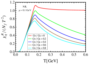
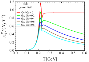
Figure 16: Resummed quark number susceptibility in (a) NJL model and (b) PNJL model at non-zero chemical potential for two flavor $(N_{f}=2)$.

Now, we can calculate quark number susceptibility (QNS) associated with the temporal part of the vector spectral function through the conserved density fluctuation as given in (40). The resummed susceptibility for a set of values of $G_{V}$ at finite quark chemical potential ($\mu=100$ MeV) is shown in Fig. 16. For positive vector coupling $G_{V}$ the denominator of (40) is always greater than unity and as a result the resummed susceptibility gets suppressed as one increases $G_{V}$. Since positive $G_{V}$ implies a repulsive interaction, the compressibility of the system decreases with increase of $G_{V}$, hence the susceptibility as seen from Fig. 16 decreases. We note that the QNS at finite $\mu$ shows an important feature around the phase transition temperature than that at $\mu=0$ Ghosh:2014zra . This is due to the fact that the mean fields ($X=\sigma,\ \,\Phi$ and $\bar{\Phi}$) which implicitly depend on $\mu$ contributes strongly as the change of these fields are most significant around the transition region. This feature could be important in the perspective of FAIR scenario where a hot but very dense matter is expected to be created. Using (10) one can compute the temporal Euclidean correlation function associated with the QNS as ${\cal G}^{E}_{00}(\tau T)/T=-\chi^{R}_{q}(T)$, which does not depend on $\tau$ but on $T$. This study could also provide useful information to future LQCD calculation at finite $\mu$.

6 Conclusion

In the present work, the behavior of the vector meson correlation function and its spectral representation, and various physical quantities associated with the spectral representation, in a hot and dense environment, have been studied within the effective model framework, viz. NJL and PNJL model. PNJL model contains additional nonperturbative information through Polyakov Loop fields than NJL model. In addition to this nonperturbative effect of Polyakov Loop, the repulsive isoscalar-vector interaction is also considered. The influence of such interaction on the correlator and its spectral representation in a hot and dense medium has been obtained using ring resummation known as Random Phase Approximation. The incorporation of vector interaction is important, in particular, for various spectral properties of the system at non-zero chemical potential. However, the value of the vector coupling strength is difficult to fix from the mass scale which is higher than the maximum energy scale $\Lambda$ of the effective theory. So, we have made different choices of this vector coupling strength to understand qualitatively its effect on the various quantities we have computed.

In absence of the isoscalar-vector interaction, the static spectral function and the correlation function in NJL model become quantitatively equivalent to those of free field theory. In case of PNJL these quantities are different from both free and NJL case because of the presence of the nonperturbative Polyakov Loop fields that suppress the color degrees of freedom in the deconfined phase just above $T_{c}$. This suggests that some nontrivial correlation exist among the color charges in the deconfined phase. As an important consequence, the nonperturbative dilepton production rate is enhanced in the deconfined phase compared to the leading order perturbative rate. We note that the Euclidean correlation function and the nonperturbative rate with zero chemical potential agree well with the available LQCD data in quenched approximation. We also discussed these quantities in presence of finite chemical potential and external momentum which could provide useful information if, in future, LQCD computes them at finite chemical potential and external momentum.

In presence of the isoscalar-vector interaction, appropriate for hot but very dense medium likely to be created at FAIR GSI, it is found that the color degrees of freedoms are, further, suppressed up to a moderate value of the temperature above the critical temperature implying a stronger correlation among the color charges in the deconfined phase. The correlation function, spectral function and its spectral property, e.g., the low mass dilepton rate are strongly affected in PNJL case than NJL case. We also note that the response to the conserved number density fluctuation at finite chemical potential exhibits an interesting characteristic around the phase transition temperature than that at vanishing chemical potential. This is because the mean fields (Polyakov Loop fields and condensates etc.) depend implicitly on chemical potential and so their variations are most significant around the transition region, in particular for PNJL model. Finally, some of our results presented in this work can be tested when LQCD computes them, in future, with the inclusion of the dynamical fermions.

- (1) B. Muller, “The Physics Of The Quark - Gluon Plasma,” Lect. Notes Phys. 225, 1 (1985).
- (2) U. W. Heinz and M. Jacob, “Evidence for a new state of matter: An Assessment of the results from the CERN lead beam program,” nucl-th/0002042.
- (3) I. Arsene et al. [BRAHMS Collaboration], “Quark gluon plasma and color glass condensate at RHIC? The Perspective from the BRAHMS experiment,” Nucl. Phys. A 757, 1 (2005) [nucl-ex/0410020].
- (4) B. B. Back, M. D. Baker, M. Ballintijn, D. S. Barton, B. Becker, R. R. Betts, A. A. Bickley and R. Bindel et al., “The PHOBOS perspective on discoveries at RHIC,” Nucl. Phys. A 757, 28 (2005) [nucl-ex/0410022].
- (5) J. Adams et al. [STAR Collaboration], “Experimental and theoretical challenges in the search for the quark gluon plasma: The STAR Collaboration’s critical assessment of the evidence from RHIC collisions,” Nucl. Phys. A 757, 102 (2005) [nucl-ex/0501009].
- (6) K. Adcox et al. [PHENIX Collaboration], “Formation of dense partonic matter in relativistic nucleus-nucleus collisions at RHIC: Experimental evaluation by the PHENIX collaboration,” Nucl. Phys. A 757, 184 (2005) [nucl-ex/0410003].
- (7) F. Carminati et al. [ALICE Collaboration], “ALICE: Physics performance report, volume I,” J. Phys. G 30, 1517 (2004).
- (8) B. Alessandro et al. [ALICE Collaboration], “ALICE: Physics performance report, volume II,” J. Phys. G 32, 1295 (2006).
- (9) B. Friman, C. Hohne, J. Knoll, S. Leupold, J. Randrup, R. Rapp and P. Senger, “The CBM physics book: Compressed baryonic matter in laboratory experiments,” Lect. Notes Phys. 814, 1 (2011).
- (10) A. Adare et al. [PHENIX Collaboration], “Detailed measurement of the pair continuum in and Au+Au collisions at GeV and implications for direct photon production,” Phys. Rev. C 81, 034911 (2010) [arXiv:0912.0244 [nucl-ex]].
- (11) S. S. Adler et al. [PHENIX Collaboration], “Measurement of direct photon production in p + p collisions at -GeV,” Phys. Rev. Lett. 98, 012002 (2007) [hep-ex/0609031].
- (12) A. Adare et al. [PHENIX Collaboration], “Scaling properties of azimuthal anisotropy in Au+Au and Cu+Cu collisions at = 200-GeV,” Phys. Rev. Lett. 98, 162301 (2007) [nucl-ex/0608033].
- (13) K. Adcox et al. [PHENIX Collaboration], “Suppression of hadrons with large transverse momentum in central Au+Au collisions at = 130-GeV,” Phys. Rev. Lett. 88, 022301 (2002) [nucl-ex/0109003].
- (14) K. Adcox et al. [PHENIX Collaboration], “Measurement of the Lambda and anti-Lambda particles in Au+Au collisions at -GeV,” Phys. Rev. Lett. 89, 092302 (2002) [nucl-ex/0204007].
- (15) S. S. Adler et al. [PHENIX Collaboration], “Scaling properties of proton and anti-proton production in -GeV Au+Au collisions,” Phys. Rev. Lett. 91, 172301 (2003) [nucl-ex/0305036].
- (16) T. Chujo [PHENIX Collaboration], “Results on identified hadrons from the PHENIX experiment at RHIC,” Nucl. Phys. A 715, 151 (2003) [nucl-ex/0209027].
- (17) A. Adare et al. [PHENIX Collaboration], “Energy Loss and Flow of Heavy Quarks in Au+Au Collisions at -GeV,” Phys. Rev. Lett. 98, 172301 (2007) [nucl-ex/0611018].
- (18) B. I. Abelev et al. [STAR Collaboration], “Erratum: Transverse momentum and centrality dependence of high- non-photonic electron suppression in Au+Au collisions at GeV,” Phys. Rev. Lett. 98, 192301 (2007) [Erratum-ibid. 106, 159902 (2011)] [nucl-ex/0607012].
- (19) K. Aamodt et al. [ALICE Collaboration], “Charged-particle multiplicity density at mid-rapidity in central Pb-Pb collisions at TeV,” Phys. Rev. Lett. 105, 252301 (2010) [arXiv:1011.3916 [nucl-ex]].
- (20) K. Aamodt et al. [ALICE Collaboration], “Elliptic flow of charged particles in Pb-Pb collisions at 2.76 TeV,” Phys. Rev. Lett. 105, 252302 (2010) [arXiv:1011.3914 [nucl-ex]].
- (21) K. Aamodt et al. [ALICE Collaboration], “Suppression of Charged Particle Production at Large Transverse Momentum in Central Pb–Pb Collisions at TeV,” Phys. Lett. B 696, 30 (2011) [arXiv:1012.1004 [nucl-ex]].
- (22) G. Aad et al. [ATLAS Collaboration], “Observation of a Centrality-Dependent Dijet Asymmetry in Lead-Lead Collisions at TeV with the ATLAS Detector at the LHC,” Phys. Rev. Lett. 105, 252303 (2010) [arXiv:1011.6182 [hep-ex]].
- (23) S. Chatrchyan et al. [CMS Collaboration], “Observation and studies of jet quenching in PbPb collisions at nucleon-nucleon center-of-mass energy = 2.76 TeV,” Phys. Rev. C 84, 024906 (2011) [arXiv:1102.1957 [nucl-ex]].
- (24) D. Forster, Hydrodynamics Fluctuation, Broken Symmetry and Correlation Function (Benjamin/Cummings, Menlo Park,CA, 1975);
- (25) H. B. Callen and T. A. Welton, “Irreversibility and generalized noise,” Phys. Rev. 83, 34 (1951).
- (26) R. Kubo, “Statistical mechanical theory of irreversible processes. 1. General theory and simple applications in magnetic and conduction problems,” J. Phys. Soc. Jap. 12, 570 (1957).
- (27) R. M. Davidson and E. Ruiz Arriola, “Mesonic correlation functions in the NJL model with vector mesons,” Phys. Lett. B 359, 273 (1995).
- (28) A. Andronic, P. Braun-Munzinger, J. Stachel and M. Winn, “Interacting hadron resonance gas meets lattice QCD,” Phys. Lett. B 718, 80 (2012) [arXiv:1201.0693 [nucl-th]].
- (29) P. Huovinen and P. Petreczky, “QCD Equation of State and Hadron Resonance Gas,” Nucl. Phys. A 837, 26 (2010) [arXiv:0912.2541 [hep-ph]].
- (30) J. I. Kapusta and C. Gale, Finite Temperature Field Theory Principle and Applications (Cambridge University Press, Cambridge, 1996), 2nd ed.
- (31) M. LeBellac, Thermal Field Theory (Cambridge University Press, Cambridge, 1996), 1st ed.
- (32) C. Gale and J. I. Kapusta, “Vector dominance model at finite temperature,” Nucl. Phys. B 357, 65 (1991).
- (33) M. G. Mustafa, A. Schafer and M. H. Thoma, “Nonperturbative dilepton production from a quark gluon plasma,” Phys. Rev. C 61, 024902 (2000) [hep-ph/9908461].
- (34) S. Ghosh, S. Sarkar and S. Mallik, “Analytic structure of rho meson propagator at finite temperature,” Eur. Phys. J. C 70, 251 (2010) [arXiv:0911.3504 [hep-ph]].
- (35) H.-T. Ding, A. Francis, O. Kaczmarek, F. Karsch, E. Laermann and W. Soeldner, “Thermal dilepton rate and electrical conductivity: An analysis of vector current correlation functions in quenched lattice QCD,” Phys. Rev. D 83, 034504 (2011) [arXiv:1012.4963 [hep-lat]].
- (36) O. Kaczmarek and A. Francis, “Electrical conductivity and thermal dilepton rate from quenched lattice QCD,” J. Phys. G 38, 124178 (2011) [arXiv:1109.4054 [hep-lat]].
- (37) A. Francis and O. Kaczmarek, “On the temperature dependence of the electrical conductivity in hot quenched lattice QCD,” Prog. Part. Nucl. Phys. 67, 212 (2012) [arXiv:1112.4802 [hep-lat]].
- (38) S. Datta, F. Karsch, P. Petreczky and I. Wetzorke, “Behavior of charmonium systems after deconfinement,” Phys. Rev. D 69, 094507 (2004) [hep-lat/0312037].
- (39) G. Aarts, C. Allton, J. Foley, S. Hands and S. Kim, “Spectral functions at small energies and the electrical conductivity in hot, quenched lattice QCD,” Phys. Rev. Lett. 99, 022002 (2007) [hep-lat/0703008 [HEP-LAT]].
- (40) G. Aarts and J. M. Martinez Resco, “Transport coefficients, spectral functions and the lattice,” JHEP 0204, 053 (2002) [hep-ph/0203177].
- (41) G. Aarts and J. M. Martinez Resco, “Ward identity and electrical conductivity in hot QED,” JHEP 0211, 022 (2002) [hep-ph/0209048].
- (42) A. Amato, G. Aarts, C. Allton, P. Giudice, S. Hands and J. I. Skullerud, “Electrical conductivity of the quark-gluon plasma across the deconfinement transition,” Phys. Rev. Lett. 111, 172001 (2013) [arXiv:1307.6763 [hep-lat]].
- (43) F. Karsch, E. Laermann, P. Petreczky, S. Stickan and I. Wetzorke, “A Lattice calculation of thermal dilepton rates,” Phys. Lett. B 530, 147 (2002) [hep-lat/0110208].
- (44) G. Aarts and J. M. Martinez Resco, “Continuum and lattice meson spectral functions at nonzero momentum and high temperature,” Nucl. Phys. B 726, 93 (2005) [hep-lat/0507004].
- (45) F. Karsch, M. G. Mustafa and M. H. Thoma, “Finite temperature meson correlation functions in HTL approximation,” Phys. Lett. B 497, 249 (2001) [hep-ph/0007093].
- (46) E. Braaten, R. D. Pisarski and T. C. Yuan, “Production of Soft Dileptons in the Quark - Gluon Plasma,” Phys. Rev. Lett. 64, 2242 (1990).
- (47) C. Greiner, N. Haque, M. G. Mustafa and M. H. Thoma, “Low Mass Dilepton Rate from the Deconfined Phase,” Phys. Rev. C 83, 014908 (2011) [arXiv:1010.2169 [hep-ph]].
- (48) P. Chakraborty, M. G. Mustafa and M. H. Thoma, “Quark number susceptibility, thermodynamic sum rule, and hard thermal loop approximation,” Phys. Rev. D 68, 085012 (2003) [hep-ph/0303009].
- (49) P. Chakraborty, M. G. Mustafa and M. H. Thoma, “Quark number susceptibility in hard thermal loop approximation,” Eur. Phys. J. C 23, 591 (2002) [hep-ph/0111022].
- (50) P. Chakraborty, M. G. Mustafa and M. H. Thoma, “Chiral susceptibility in hard thermal loop approximation,” Phys. Rev. D 67, 114004 (2003) [hep-ph/0210159].
- (51) M. Laine, A. Vuorinen and Y. Zhu, “Next-to-leading order thermal spectral functions in the perturbative domain,” JHEP 1109, 084 (2011) [arXiv:1108.1259 [hep-ph]].
- (52) P. Czerski, “HTL meson correlation functions at finite momentum and chemical potential,” Nucl. Phys. A 807, 11 (2008).
- (53) P. Czerski, “Pseudoscalar Meson Temporal Correlation Function in HTL approach,” Int. J. Mod. Phys. A 22, 672 (2007) [hep-ph/0608134].
- (54) W. M. Alberico, A. Beraudo, P. Czerski and A. Molinari, “Finite momentum meson correlation functions in a QCD plasma,” Nucl. Phys. A 775, 188 (2006) [hep-ph/0605060].
- (55) W. M. Alberico, A. Beraudo and A. Molinari, “Meson correlation functions in a QCD plasma,” Nucl. Phys. A 750, 359 (2005) [hep-ph/0411346].
- (56) P. B. Arnold, G. D. Moore and L. G. Yaffe, “Transport coefficients in high temperature gauge theories. 1. Leading log results,” JHEP 0011, 001 (2000) [hep-ph/0010177].
- (57) P. B. Arnold, G. D. Moore and L. G. Yaffe, “Transport coefficients in high temperature gauge theories. 2. Beyond leading log,” JHEP 0305, 051 (2003) [hep-ph/0302165].
- (58) Y. Burnier and M. Laine, “Massive vector current correlator in thermal QCD,” JHEP 1211, 086 (2012) [arXiv:1210.1064 [hep-ph]].
- (59) M. Laine and M. Vepsalainen, “Mesonic correlation lengths in high temperature QCD,” JHEP 0402, 004 (2004) [hep-ph/0311268].
- (60) T. H. Hansson and I. Zahed, “Hadronic correlators in hot QCD,” Nucl. Phys. B 374, 277 (1992).
- (61) N. Haque, J. O. Andersen, M. G. Mustafa, M. Strickland and N. Su, “Three-loop HTLpt Pressure and Susceptibilities at Finite Temperature and Density,” Phys. Rev. D 89, 061701 (2014) [arXiv:1309.3968 [hep-ph]].
- (62) N. Haque, A. Bandyopadhyay, J. O. Andersen, M. G. Mustafa, M. Strickland and N. Su, “Three-loop HTLpt thermodynamics at finite temperature and chemical potential,” JHEP 1405, 027 (2014) [arXiv:1402.6907 [hep-ph]].
- (63) N. Haque, M. G. Mustafa and M. Strickland, “Quark Number Susceptibilities from Two-Loop Hard Thermal Loop Perturbation Theory,” JHEP 1307, 184 (2013) [arXiv:1302.3228 [hep-ph]].
- (64) N. Haque, M. G. Mustafa and M. Strickland, Phys. Rev. D 87, no. 10, 105007 (2013) [arXiv:1212.1797 [hep-ph]].
- (65) B. He, H. Li, C. M. Shakin and Q. Sun, “Comparison of temperature dependent hadronic current correlation functions calculated in lattice simulations of QCD and with a chiral Lagrangian model,” Phys. Rev. C 67, 065203 (2003) [hep-ph/0302105].
- (66) B. He, H. Li, C. M. Shakin and Q. Sun, “Calculation of the pseudoscalar isoscalar hadronic current correlation functions of the quark gluon plasma,” Phys. Rev. D 67, 014022 (2003) [hep-ph/0210387].
- (67) B. He, H. Li, C. M. Shakin and Q. Sun, “Calculation of temperature dependent hadronic correlation functions of pseudoscalar and vector currents,” Phys. Rev. D 67, 114012 (2003) [hep-ph/0212345].
- (68) T. Kunihiro, “Quark number susceptibility and fluctuations in the vector channel at high temperatures,” Phys. Lett. B 271, 395 (1991).
- (69) M. Oertel, M. Buballa and J. Wambach, “Meson loop effects in the NJL model at zero and nonzero temperature,” Phys. Atom. Nucl. 64, 698 (2001) [Yad. Fiz. 64, 757 (2001)] [hep-ph/0008131].
- (70) K. Fukushima, “Chiral effective model with the Polyakov loop,” Phys. Lett. B 591, 277 (2004) [hep-ph/0310121].
- (71) K. Fukushima, “Relation between the Polyakov loop and the chiral order parameter at strong coupling,” Phys. Rev. D 68, 045004 (2003) [hep-ph/0303225].
- (72) R. D. Pisarski, “Quark gluon plasma as a condensate of SU(3) Wilson lines,” Phys. Rev. D 62, 111501 (2000) [hep-ph/0006205].
- (73) A. Dumitru and R. D. Pisarski, “Degrees of freedom and the deconfining phase transition,” Phys. Lett. B 525, 95 (2002) [hep-ph/0106176].
- (74) A. Dumitru and R. D. Pisarski, “Two point functions for SU(3) Polyakov loops near T(c),” Phys. Rev. D 66, 096003 (2002) [hep-ph/0204223].
- (75) A. Dumitru, Y. Hatta, J. Lenaghan, K. Orginos and R. D. Pisarski, “Deconfining phase transition as a matrix model of renormalized Polyakov loops,” Phys. Rev. D 70, 034511 (2004) [hep-th/0311223].
- (76) D. J. Gross, R. D. Pisarski and L. G. Yaffe, “QCD and Instantons at Finite Temperature,” Rev. Mod. Phys. 53, 43 (1981).
- (77) A. Gocksch and R. D. Pisarski, “Partition function for the eigenvalues of the Wilson line,” Nucl. Phys. B 402, 657 (1993) [hep-ph/9302233].
- (78) N. Weiss, “The Effective Potential for the Order Parameter of Gauge Theories at Finite Temperature,” Phys. Rev. D 24, 475 (1981).
- (79) N. Weiss, “The Wilson Line in Finite Temperature Gauge Theories,” Phys. Rev. D 25, 2667 (1982).
- (80) S. K. Ghosh, T. K. Mukherjee, M. G. Mustafa and R. Ray, “Susceptibilities and speed of sound from PNJL model,” Phys. Rev. D 73, 114007 (2006) [hep-ph/0603050].
- (81) S. Mukherjee, M. G. Mustafa and R. Ray, “Thermodynamics of the PNJL model with nonzero baryon and isospin chemical potentials,” Phys. Rev. D 75, 094015 (2007) [hep-ph/0609249].
- (82) S. K. Ghosh, T. K. Mukherjee, M. G. Mustafa and R. Ray, “PNJL model with a Van der Monde term,” Phys. Rev. D 77, 094024 (2008) [arXiv:0710.2790 [hep-ph]].
- (83) C. Ratti, M. A. Thaler and W. Weise, “Phases of QCD: Lattice thermodynamics and a field theoretical model,” Phys. Rev. D 73, 014019 (2006) [hep-ph/0506234].
- (84) S. K. Ghosh, A. Lahiri, S. Majumder, M. G. Mustafa, S. Raha and R. Ray, “Quark Number Susceptibility : Revisited with Fluctuation-Dissipation Theorem in mean field theories,” Phys. Rev. D 90, 054030 (2014) [arXiv:1407.7203 [hep-ph]].
- (85) H. Hansen, W. M. Alberico, A. Beraudo, A. Molinari, M. Nardi and C. Ratti, “Mesonic correlation functions at finite temperature and density in the Nambu-Jona-Lasinio model with a Polyakov loop,” Phys. Rev. D 75, 065004 (2007) [hep-ph/0609116].
- (86) P. Deb, A. Bhattacharyya, S. Datta and S. K. Ghosh, “Mesonic Excitations of QGP: Study with an Effective Model,” Phys. Rev. C 79, 055208 (2009) [arXiv:0901.1992 [nucl-th]].
- (87) S. Carignano, D. Nickel and M. Buballa, “Influence of vector interaction and Polyakov loop dynamics on inhomogeneous chiral symmetry breaking phases,” Phys. Rev. D 82, 054009 (2010) [arXiv:1007.1397 [hep-ph]].
- (88) K. Kashiwa, H. Kouno, T. Sakaguchi, M. Matsuzaki and M. Yahiro, “Chiral phase transition in an extended NJL model with higher-order multi-quark interactions,” Phys. Lett. B 647, 446 (2007) [nucl-th/0608078].
- (89) Y. Sakai, K. Kashiwa, H. Kouno, M. Matsuzaki and M. Yahiro, “Vector-type four-quark interaction and its impact on QCD phase structure,” Phys. Rev. D 78, 076007 (2008) [arXiv:0806.4799 [hep-ph]].
- (90) K. Fukushima, “Phase diagrams in the three-flavor Nambu-Jona-Lasinio model with the Polyakov loop,” Phys. Rev. D 77, 114028 (2008) [Erratum-ibid. D 78, 039902 (2008)] [arXiv:0803.3318 [hep-ph]].
- (91) K. Fukushima, “Critical surface in hot and dense QCD with the vector interaction,” Phys. Rev. D 78, 114019 (2008) [arXiv:0809.3080 [hep-ph]].
- (92) R.Z. Denke, J. C. Macias, M. B. Pinto, “Critical Line Back-Bending Induced either by Finite Nc Corrections or by a Repulsive Vector Channel,” Jour. of Mod. Phys 4, 1583 (2013).
- (93) P. Jaikumar, R. Rapp and I. Zahed, “Photon and dilepton emission rates from high density quark matter,” Phys. Rev. C 65, 055205 (2002) [hep-ph/0112308].
- (94) N. Haque, M. G. Mustafa and M. H. Thoma, “Conserved Density Fluctuation and Temporal Correlation Function in HTL Perturbation Theory,” Phys. Rev. D 84, 054009 (2011) [arXiv:1103.3394 [hep-ph]].
- (95) Y. Nakahara, M. Asakawa and T. Hatsuda, “Hadronic spectral functions in lattice QCD,” Phys. Rev. D 60, 091503 (1999) [hep-lat/9905034].
- (96) M. Asakawa, T. Hatsuda and Y. Nakahara, “Maximum entropy analysis of the spectral functions in lattice QCD,” Prog. Part. Nucl. Phys. 46, 459 (2001) [hep-lat/0011040].
- (97) I. Wetzorke and F. Karsch, “Testing MEM with diquark and thermal meson correlation functions,” hep-lat/0008008.
- (98) S. P. Klevansky, “The Nambu-Jona-Lasinio model of quantum chromodynamics,” Rev. Mod. Phys. 64, 649 (1992).
- (99) T. Hatsuda and T. Kunihiro, “QCD phenomenology based on a chiral effective Lagrangian,” Phys. Rept. 247, 221 (1994) [hep-ph/9401310].
- (100) M. Buballa, “NJL model analysis of quark matter at large density,” Phys. Rept. 407, 205 (2005) [hep-ph/0402234].
- (101) C. A. Islam, R. Abir, M. G. Mustafa, R. Ray and S. K. Ghosh, “The consequences of colorsingletness, Polyakov Loop and symmetry on a quark–gluon gas,” J. Phys. G 41, 025001 (2014).
- (102) Ashok Das, Finite Temperature Field Theory, World scientific.
- (103) C. Gale, Y. Hidaka, S. Jeon, S. Lin, J.-F. Paquet, R. D. Pisarski, D. Satow and V. V. Skokov et al., “Production and Elliptic Flow of Dileptons and Photons in the semi-Quark Gluon Plasma,” arXiv:1409.4778 [hep-ph].
- (104) A. Bazavov, T. Bhattacharya, M. Cheng, C. DeTar, H. T. Ding, S. Gottlieb, R. Gupta and P. Hegde et al., “The chiral and deconfinement aspects of the QCD transition,” Phys. Rev. D 85, 054503 (2012) [arXiv:1111.1710 [hep-lat]].
- (105) P. Petreczky, “Numerical study of hot strongly interacting matter,” J. Phys. Conf. Ser. 402, 012036 (2012) [arXiv:1204.4414 [hep-lat]].
- (106) S. Borsanyi et al. [Wuppertal-Budapest Collaboration], “Is there still any mystery in lattice QCD? Results with physical masses in the continuum limit III,” JHEP 1009, 073 (2010) [arXiv:1005.3508 [hep-lat]].