LU TP 14-38

arXiv:1411.6384 [hep-lat]

Revised January 2015

Finite Volume at Two-loops
in Chiral Perturbation Theory Johan Bijnens and Thomas Rössler
Department of Astronomy and Theoretical Physics, Lund University,

Sölvegatan 14A, SE 223-62 Lund, Sweden

We calculate the finite volume corrections to meson masses and decay constants in two and three flavour Chiral Perturbation Theory to two-loop order. The analytical results are compared with the existing result for the pion mass in two-flavour ChPT and the partial results for the other quantities. We present numerical results for all quantities.

1 Introduction

Lattice QCD now provides good calculations of a number of quantities relevant for low-energy particle physics as reviewed in [1]. These need several extrapolations, in the quark masses, in the lattice spacing, in the lattice size and in lattice artefacts. Chiral Perturbation Theory (ChPT) [2, 3, 4] provides guidance for all of these extrapolations. In particular, it can be used to estimate the corrections due to the finite lattice size. This was introduced by Gasser and Leutwyler in [5, 6, 7]. This is an alternative method compared to the one introduced by Lüscher [8] where the leading finite size corrections can be derived using the scattering amplitude.

In this paper we will restrict ourselves to the $p$-regime with $m_{\pi}L>>1$. We will not do the all order integration over the zero mode as is necessary in the so-called $\epsilon$-regime [5, 6, 7]. The finite volume corrections to the mass and decay constant in the equal mass case to one-loop order were calculated in these original papers. Since then, there have been many studies of finite size effects at one-loop order in ChPT, in particular the masses and decay constants to that order were derived in [9] and [10].

In infinite volume the ChPT expressions for masses and decay constants are known for all relevant cases and including a number of extensions as e.g. partially quenched ChPT to two-loop order. This is reviewed in [11]. There exist a few two-loop calculations at finite volume in ChPT. The mass in two-flavour ChPT was studied in [12] and the quark-anti quark vacuum expectation value in three-flavour ChPT in [13], the latter can be extended to the $\epsilon$-regime [14].

The main purpose of this paper is to provide the two-loop finite volume expressions in two and three-flavour ChPT for the masses and decay constants. The extension to partially quenched ChPT is planned for future work. The main reason this was not done earlier is the complexity of the sunset integral at finite volume. The needed integrals have been recently worked out in [15]. We will use their expressions extensively. Our expressions are valid in the frame with $\vec{p}=0$, often called the center-of-mass frame. In the so-called moving frames or with twisted boundary conditions there will be additional terms.

Some preliminary numerical results were reported in [16]. We find the typical $e^{-m_{\pi}L}$ behaviour for most quantities as expected. The corrections for the pion mass and decay constant are significant at the present lattice size and precision in lattice QCD calculations. The corrections for the kaon decay constant are needed but are not quite as large. The kaon mass has corrections below 1% and the corrections for the eta mass and decay constant turn out to be negligible at present precision. These results are in qualitative agreement with the earlier work.

We give a short list of references for ChPT and discuss some small points in Sect. 2. The definitions of the integrals we use and how they relate to the results in [15] is given in Sect. 3. The next section contains our first major results. The full finite volume correction to the pion mass and decay constant to two-loop order in ChPT. Sect. 5 contains the results for the three-flavour case for pion, kaon and eta for both the mass and decay constant but the large two-loop order formulas are collected in the appendices. The detailed numerical discussion of our results is in Sect. 6.

2 Chiral Perturbation Theory

An introduction to ChPT can be found in [17] and in the two-loop review [11]. The lowest order and $p^{4}$-Lagrangian can be found in [3] and [4] for the two and three flavour case respectively. The order $p^{6}$ Lagrangian is given in [18]. We use the standard renormalization scheme in ChPT. The needed part for the finite volume integrals is discussed in Sect. 3. An extensive discussion of the scheme can be found in [19] and [20]. An important comment is that the LECs do not depend on the volume [7].

We prefer to designate orders by the $p$-counting order at which the diagram appears. Thus we refer to order $p^{2}$, order $p^{4}$ or one-loop order and order $p^{6}$ or two-loop order and include in the terminology one- or two-loop order also the diagrams with fewer loops but the same order in $p$-counting.

We present the formulas here in terms of the physical infinite volume masses and decay constants.

3 Comments on the finite volume integrals

The loop integrals at finite volume at one-loop are well known. The difference with infinite volume is that there is a sum over discrete momenta in every direction with a finite size rather than a continuous integral. The use of the Poisson summation formula allows to identify the infinite volume part and the finite volume corrections. The remainder can be done in two ways. For one-loop tadpole integrals the first one was introduced in the original work [5, 6, 7] and one remains with a sum over Bessel functions, that for large $ML$ converges fast. The other method can be found in [9] and one remains with an integral over a Jacobi theta function, this method can be used for small and medium $ML$ as well. The extensions to other one-loop integrals can be done in both cases by combining propagators with Feynman parameters. The first method was extended to the equal mass two-loop sunset integral in [12]. The general mass case was then done in both methods in [15]. The methods are explained in detail in [15] for both the one and two-loop case. Note that here we use Minkowski notation for the integrals.

The tadpole integrals $A$ and $A_{\mu\nu}$ are defined via

$$\left\{A(m^{2}),A_{\mu\nu}(m^{2})\right\}=\frac{1}{i}\int_{V}\frac{d^{d}r}{(2\pi)^{d}}\frac{\left\{1,r_{\mu}r_{\nu}\right\}}{(r^{2}-m^{2})}\,.$$ (1)

The $B^{0}$ tadpole integrals are defined similarly with a doubled propagator, alternatively as the derivative w.r.t. $m^{2}$ of the $A$-tadpoles. The subscript $V$ on the integral indicates that the integral is a discrete sum over the three spatial components and an integral over the remainder. At finite volume, there are more Lorentz-structures possible. We define the tensor $t_{\mu\nu}$ as the spatial part of the Minkowski metric $g_{\mu\nu}$, to express these. For the center-of-mass (cms) case this is sufficient. The needed functions for $A_{\mu\nu}$ are

$$A_{\mu\nu}(m^{2})=g_{\mu\nu}A_{22}(m^{2})+t_{\mu\nu}A_{23}(m^{2})\,.$$ (2)

In infinite volume $A_{22}$ can be rewritten in terms of $A$. At finite volume, the relation is

$$dA_{22}(m^{2})+3A_{23}(m^{2})=m^{2}A(m^{2})\,.$$ (3)

This is used to remove $A_{22}$ from our expressions. In addition we do an expansion in $\epsilon$ with $d=4-2\epsilon$ via

$$A(m^{2})=\lambda_{0}\frac{m^{2}}{16\pi^{2}}+\overline{A}(m^{2})+A^{V}(m^{2})+\epsilon\left(A^{\epsilon}(m^{2})+A^{V\epsilon}(m^{2})\right)+\cdots\,.$$ (4)

with $\lambda_{0}=\frac{1}{\epsilon}+\log(4\pi)+1-\gamma$ and similarly for the other one-loop integrals. $\lambda_{0}$ corresponds to the usual $\overline{MS}$ variant used in ChPT. Doing the renormalization introduces a subtraction point dependence which corresponds to using for $\overline{A}(m^{2})$ and $\overline{B}^{0}(m^{2})$

$$\overline{A}(m^{2})=\frac{-m^{2}}{16\pi^{2}}\log\frac{m^{2}}{\mu^{2}}\,,\quad\overline{B}^{0}(m^{2})=\frac{-1}{16\pi^{2}}\left(\log\frac{m^{2}}{\mu^{2}}+1\right)\,.$$ (5)

The sunset integrals are defined as

$$\left\{H,H_{\mu},H_{\mu}^{s},H_{\mu\nu},H_{\mu\nu}^{rs},H_{\mu\nu}^{ss}\right\}(m_{1}^{2},m_{2}^{2},m_{3}^{2},p)=$$ (6)

$$\frac{1}{i^{2}}\int_{V}\frac{d^{d}r}{(2\pi)^{d}}\frac{d^{d}s}{(2\pi)^{d}}\frac{\left\{1,r_{\mu},s_{\mu},r_{\mu}r_{\nu},r_{\mu}s_{\nu},s_{\mu}s_{\nu}\right\}}{\left(r^{2}-m_{1}^{2}\right)\left(s^{2}-m_{2}^{2}\right)\left((r+s-p)^{2}-m_{3}^{2}\right)}\,.$$

The subscript $V$ again indicates that the spatial dimensions are a discrete sum rather than an integral. The conventions correspond to those in infinite volume of [21]. The interchange $r,m_{1}^{2}\leftrightarrow s,m_{2}^{2}$ shows that $H^{s}_{\mu},H^{ss}_{\mu\nu}$ are related directly to $H^{r}_{\mu},H^{rr}_{\mu\nu}$. $H^{rs}_{\mu\nu}$ can also be related to $H_{\mu\nu}$ using the trick shown in [21] which remains valid at finite volume in the cms frame [15].

In the cms frame we define the functions

$$H_{\mu} = p_{\mu}H_{1}\,$$ (7)

$$H_{\mu\nu} = p_{\mu}p_{\nu}H_{21}+g_{\mu\nu}H_{22}+t_{\mu\nu}H_{27}\,.$$

The arguments of all functions in the cms frame are $(m_{1}^{2},m_{2}^{2},m_{3}^{2},p^{2})$. These functions satisfy the relations, valid in finite volume [15],

$$H_{1}(m_{1}^{2},m_{2}^{2},m_{3}^{2},p^{2})+H_{1}(m_{2}^{2},m_{3}^{2},m_{1}^{2},p^{2})+H_{1}(m_{3}^{2},m_{1}^{2},m_{2}^{2},p^{2}) = H(m_{1}^{2},m_{2}^{2},m_{3}^{2},p^{2})\,,$$

$$p^{2}H_{21}+dH_{22}+3H_{27}-m_{1}^{2}H = A(m_{2}^{2})A(m_{3}^{2})\,.$$ (8)

The arguments of the sunset functions in the second relation are all $(m_{1}^{2},m_{2}^{2},m_{3}^{2},p^{2})$. These relations have been used to remove $H_{22}$ from the final result and simplify the expressions somewhat.

We now split the functions in an infinite volume part $\tilde{H}_{i}$ and a finite volume correction $\tilde{H}^{V}_{i}$ with $H_{i}=\tilde{H}_{i}+\tilde{H}^{V}_{i}$. The infinite volume part was derived in [21]. For the finite volume parts we define

$$\tilde{H}^{V} = \frac{\lambda_{0}}{16\pi^{2}}\left(A^{V}(m_{1}^{2})+A^{V}(m_{2}^{2})+A^{V}(m_{3}^{2})\right)+\frac{1}{16\pi^{2}}\left(A^{V\epsilon}(m_{1}^{2})+A^{V\epsilon}(m_{2}^{2})+A^{V\epsilon}(m_{3}^{2})\right)$$

$$+H^{V}\,,$$

$$\tilde{H}^{V}_{1} = \frac{\lambda_{0}}{16\pi^{2}}\frac{1}{2}\left(A^{V}(m_{2}^{2})+A^{V}(m_{3}^{2})\right)+\frac{1}{16\pi^{2}}\frac{1}{2}\left(A^{V\epsilon}(m_{2}^{2})+A^{V\epsilon}(m_{3}^{2})\right)+H^{V}_{1}\,,$$

$$\tilde{H}^{V}_{21} = \frac{\lambda_{0}}{16\pi^{2}}\frac{1}{3}\left(A^{V}(m_{2}^{2})+A^{V}(m_{3}^{2})\right)+\frac{1}{16\pi^{2}}\frac{1}{3}\left(A^{V\epsilon}(m_{2}^{2})+A^{V\epsilon}(m_{3}^{2})\right)+H^{V}_{21}\,,$$

$$\tilde{H}^{V}_{27} = \frac{\lambda_{0}}{16\pi^{2}}\left(A^{V}_{23}(m_{1}^{2})+\frac{1}{3}A_{23}(m_{2}^{2})+\frac{1}{3}A^{V}_{23}(m_{3}^{2})\right)$$ (9)

$$+\frac{1}{16\pi^{2}}\left(A^{V\epsilon}_{23}(m_{1}^{2})+\frac{1}{3}A^{V\epsilon}_{23}(m_{2}^{2})+\frac{1}{3}A^{V\epsilon}_{23}(m_{3}^{2})\right)+H^{V}_{27}\,,$$

Note that the finite parts are defined slightly different compared to the infinite volume definition in [21]. Here we have pulled out the extra parts with $A^{V\epsilon}$. These functions cancel in the final result. We will also use the derivatives w.r.t. $p^{2}$ of the sunset integrals. These we denote with and extra prime, $H^{V\prime}_{i}\equiv(\partial/\partial p^{2})H^{V}_{i}$.

The functions $H^{V}_{i}$ can be computed with the methods of [15]. They correspond to adding the parts labeled with $G$ and $H$ in Sect. 4.3 and the part of Sect. 4.4 in [15]. We have in addition added the derivatives w.r.t. $p^{2}$ for all the integrals and checked the analytical results with numerical differentiation.

For all cases discussed we have done checks that both methods, via Bessel or Jacobi theta functions, give the same results.

4 Two-flavour results

The diagrams needed to obtain the mass are shown in Fig. 1.

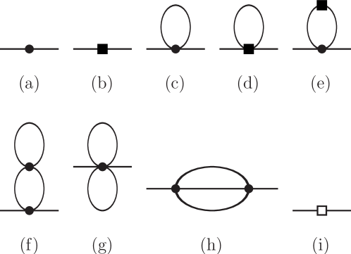
Figure 1: The Feynman diagrams needed for the mass calculation. A dot indicates a vertex of order $p^{2}$, a filled box of order $p^{4}$ and an open box of order $p^{6}$.

We write the result for the mass at finite volume in the form

$$m_{\pi}^{V2}=m_{\pi}^{2}+\Delta^{V}\!m^{2}_{\pi}\,,\quad\Delta^{V}\!m^{2}_{\pi}=\Delta^{V}\!m^{2(4)}_{\pi}+\Delta^{V}\!m^{2(6)}_{\pi}\,.$$ (10)

$m_{\pi}^{2}$ and $F_{\pi}$ denote the infinite volume physical pion mass and decay constant. We have reproduced the expression for the infinite volume mass derived in [22, 23, 24]. The extra parts due to the finite volume are

$$F_{\pi}^{2}\Delta^{V}\!m^{2(4)}_{\pi} = -\frac{1}{2}m_{\pi}^{2}{A}^{V}(m_{\pi}^{2})\,,$$

$$F_{\pi}^{4}\Delta^{V}\!m^{2(6)}_{\pi} = m_{\pi}^{4}{A}^{V}(m_{\pi}^{2})\,\Big{(}-l_{4}^{r}+5\,l_{3}^{r}+8\,l_{2}^{r}+14\,l_{1}^{r}\Big{)}+m_{\pi}^{2}{A}_{23}^{V}(m_{\pi}^{2})\,\Big{(}-12\,l_{2}^{r}-6\,l_{1}^{r}\Big{)}$$ (11)

$$+{A}^{V}(m_{\pi}^{2})\,\Big{(}13/12\,\frac{1}{16\pi^{2}}\,m_{\pi}^{4}-7/4\,\overline{A}(m_{\pi}^{2})\,m_{\pi}^{2}\Big{)}+{A}^{V}(m_{\pi}^{2})^{2}\,\Big{(}-3/8\,m_{\pi}^{2}\Big{)}$$

$$+{A}^{V}(m_{\pi}^{2})\,{B}^{0V}(m_{\pi}^{2})\,\Big{(}1/4\,m_{\pi}^{4}\Big{)}+{H}^{V}(m_{\pi}^{2},m_{\pi}^{2},m_{\pi}^{2},m_{\pi}^{2})\,\Big{(}5/6\,m_{\pi}^{4}\Big{)}$$

$$+{H}_{21}^{V}(m_{\pi}^{2},m_{\pi}^{2},m_{\pi}^{2},m_{\pi}^{2})\,\Big{(}3\,m_{\pi}^{4}\Big{)}+{H}_{27}^{V}(m_{\pi}^{2},m_{\pi}^{2},m_{\pi}^{2},m_{\pi}^{2})\,\Big{(}-3\,m_{\pi}^{2}\Big{)}\,.$$

$\Delta^{V}\!m^{2(4)}_{\pi}$ agrees with the results of [5]. The comparison of $\Delta^{V}m^{2(6)}_{\pi}$ with the result in [12] is not quite so simple. The reason is that the splitting in parts has been done very differently there and here. However, we agree on the sunset part, (44) in [12] and on the part that has $l_{i}^{r}$ multiplying finite volume integrals in (38) in [12]. The latter was first derived in [25]. Both their and our result are independent of the subtraction scale.

The pion decay constant is defined by

$$\langle 0|\bar{u}\gamma_{\mu}\gamma_{5}d|\pi^{-}(p)\rangle=\sqrt{2}iF_{\pi}p_{\mu}\,.$$ (12)

It can be computed by the diagrams of Fig. 1 where the outgoing meson is replaced by an insertion of the axial current. The diagrams needed for wave-function renormalization are the same as those for the mass. The calculation proceeds along the same lines as above. We reproduce the known infinite volume results of [22, 23, 24]. The decay constant at finite volume we write as

$$F_{\pi}^{V}=F_{\pi}+\Delta^{V}\!F_{\pi}\,,\quad\Delta^{V}\!F_{\pi}=\Delta^{V}\!F_{\pi}^{(4)}+\Delta^{V}\!F_{\pi}^{(6)}\,.$$ (13)

The results are:

$$F_{\pi}\Delta^{V}\!F_{\pi}^{(4)} = {A}^{V}(m_{\pi}^{2})\,,$$

$$F_{\pi}^{3}\Delta^{V}\!F_{\pi}^{(6)} = +{A}^{V}(m_{\pi}^{2})m_{\pi}^{2}\,\Big{(}3/2\,l_{4}^{r}-4\,l_{2}^{r}-7\,l_{1}^{r}\Big{)}+{A}_{23}^{V}(m_{\pi}^{2})\,\Big{(}6\,l_{2}^{r}+3\,l_{1}^{r}\Big{)}$$ (14)

$$+{A}^{V}(m_{\pi}^{2})\,\Big{(}-1/3\,\frac{1}{16\pi^{2}}\,m_{\pi}^{2}+1/2\,\overline{A}(m_{\pi}^{2})\Big{)}+{A}^{V}(m_{\pi}^{2})\,{B}^{0V}(m_{\pi}^{2})\,\Big{(}-1/2\,m_{\pi}^{2}\Big{)}$$

$$+{H}^{V}(m_{\pi}^{2},m_{\pi}^{2},m_{\pi}^{2},m_{\pi}^{2})\,\Big{(}-1/2\,m_{\pi}^{2}\Big{)}+{H}_{27}^{V}(m_{\pi}^{2},m_{\pi}^{2},m_{\pi}^{2},m_{\pi}^{2})\,\Big{(}3/2\Big{)}$$

$$+{H}^{V\prime}(m_{\pi}^{2},m_{\pi}^{2},m_{\pi}^{2},m_{\pi}^{2})\,\Big{(}5/12\,m_{\pi}^{4}\Big{)}+{H}_{21}^{V\prime}(m_{\pi}^{2},m_{\pi}^{2},m_{\pi}^{2},m_{\pi}^{2})\,\Big{(}3/2\,m_{\pi}^{4}\Big{)}$$

$$+{H}_{27}^{V\prime}(m_{\pi}^{2},m_{\pi}^{2},m_{\pi}^{2},m_{\pi}^{2})\,\Big{(}-3/2\,m_{\pi}^{2}\Big{)}\,.$$

$\Delta^{V}\!F_{\pi}^{(4)}$ agrees with the results of [5]. Here there exists no full two-loop calculation but an evaluation for the case with at most one propagator at finite volume [26]. We agree with their result for the terms containing $l_{i}^{r}$ if the term multiplying $B^{2}$ in (54) in that paper is divided by 2. Comparing with the remainder is difficult due to the very different treatment of the loop integrals.

5 Three-flavour results

The principle of the calculation is exactly the same as before. The diagrams needed for the mass are shown in Fig. 1. However, we now need to use the three-flavour Lagrangians and include the kaons and eta as well. As a result the expressions become much more cumbersome. Here we use as symbols, $m_{\pi}$, $m_{K}$ and $m_{\eta}$ as the physical volume pion, kaon and eta mass at infinite volume. We have rewritten all expressions as an expansion in these masses and in the physical pion decay constant at infinite volume. Given that the eta mass to lowest order is given by the Gell-Mann–Okubo relation, there is an inherent ambiguity in precisely how one writes the result in the combination of kaon and eta masses. The form of the $p^{6}$ result given here is to be used together with the form for the $p^{4}$ expressions given here as well.

The pion, kaon and eta masses at two-loop order in infinite volume are known, [21], we have reproduced that result. The finite volume corrections for the masses are given by

$$m_{i}^{V2}=m_{i}^{2}+\Delta^{V}\!m^{2}_{i}\,,\quad\Delta^{V}\!m^{2}_{i}=\Delta^{V}\!m^{2(4)}_{i}+\Delta^{V}\!m^{2(6)}_{i}\,,$$ (15)

for $i=\pi,K,\eta$. The $p^{4}$ results are:

$$F_{\pi}^{2}\Delta^{V}\!m^{2(4)}_{\pi} = {A}^{V}(m_{\pi}^{2})\,\Big{(}-1/2\,m_{\pi}^{2}\Big{)}+{A}^{V}(m_{\eta}^{2})\,\Big{(}1/6\,m_{\pi}^{2}\Big{)}\,,$$

$$F_{\pi}^{2}\Delta^{V}\!m^{2(4)}_{K} = {A}^{V}(m_{\eta}^{2})\,\Big{(}-1/4\,m_{\eta}^{2}-1/12\,m_{\pi}^{2}\Big{)}\,,$$

$$F_{\pi}^{2}\Delta^{V}\!m^{2(4)}_{\eta} = {A}^{V}(m_{\pi}^{2})\,\Big{(}1/2\,m_{\pi}^{2}\Big{)}+{A}^{V}(m_{K}^{2})\,\Big{(}-m_{\eta}^{2}-1/3\,m_{\pi}^{2}\Big{)}$$ (16)

$$+{A}^{V}(m_{\eta}^{2})\,\Big{(}8/9\,m_{K}^{2}-7/18\,m_{\pi}^{2}\Big{)}\,.$$

These agree with the expressions in [9, 10, 27]. The way in which the corrections are written is to be in agreement with the way the infinite volume result was written in [21]. The order $p^{6}$ expressions are rather large, they can be found in App. A. The contributions with at most one pion propagator at finite volume were calculated in [27] for the kaon and eta in three flavour ChPT, the expression for the pion was done in two-flavour ChPT and discussed above. We agree with the $L_{i}^{r}$ times finite volume part there. The remainder is difficult to compare due to the different treatment of the integrals.

The decay constants for the mesons are defined similarly to (12) via

$$\langle 0|\bar{u}\gamma_{\mu}\gamma_{5}d|\pi^{-}(p)\rangle = \sqrt{2}iF_{\pi}p_{\mu}\,,$$

$$\langle 0|\bar{u}\gamma_{\mu}\gamma_{5}s|K^{-}(p)\rangle = \sqrt{2}iF_{K}p_{\mu}\,,$$

$$\langle 0|\frac{1}{\sqrt{6}}\left(\bar{u}\gamma_{\mu}\gamma_{5}u+\bar{d}\gamma_{\mu}\gamma_{5}d-2\bar{s}\gamma_{\mu}\gamma_{5}s\right)|\eta(p)\rangle = \sqrt{2}iF_{\eta}p_{\mu}\,.$$ (17)

Note that since we work in the isospin limit, we use the octet axial current to define the eta decay constant.

We define

$$F_{i}^{V}=F_{i}+\Delta^{V}\!F_{i}\,,\quad\Delta^{V}\!F_{i}=\Delta^{V}\!F^{(4)}_{i}+\Delta^{V}\!F^{(6)}_{i}\,,$$ (18)

for $i=\pi,K,\eta$. The pion, kaon and eta decay constants at two-loop order in infinite volume are known, [21], we have reproduced that result. Note that we give the corrections to the decay constants here, not divided by the chiral limit decay constant as in [21]. Note the correction for the expressions for the infinite volume decay constants described in the erratum of [28]. The correct expressions can be downloaded from [29]

The order $p^{4}$ results are

$$F_{\pi}\Delta^{V}\!F_{\pi}^{(4)} = {A}^{V}(m_{\pi}^{2})+{A}^{V}(m_{K}^{2})\,\Big{(}1/2\Big{)}\,,$$

$$F_{\pi}\Delta^{V}\!F_{K}^{(4)} = {A}^{V}(m_{\pi}^{2})\,\Big{(}3/8\Big{)}+{A}^{V}(m_{K}^{2})\,\Big{(}3/4\Big{)}+{A}^{V}(m_{\eta}^{2})\,\Big{(}3/8\Big{)}\,,$$

$$F_{\pi}\Delta^{V}\!F_{\eta}^{(4)} = {A}^{V}(m_{K}^{2})\,\Big{(}3/2\Big{)}\,.$$ (19)

These agree with [9, 10, 27]. The $p^{6}$ expressions are again rather long and are given in App. B. The contributions with at most one-pion propagator at finite volume were calculated in [27] for the kaon in three flavour ChPT, the expression for the pion was done in two-flavour ChPT and discussed above. We agree with the $L_{i}^{r}$ dependent part if we multiply the contribution from the term with $B^{2}$ in (57) in by $1/2$. This is the same factor we needed to get agreement for the two-flavour pion decay constant.

6 Numerical results

For numerical input we use $F_{\pi}=92.2$ MeV, $m_{\pi}=m_{\pi^{0}}=134.9764$ MeV, the average $m_{K}$ with electromagnetic effects removed with the estimate of [30], $m_{K}=494.53$ MeV, and $m_{\eta}=547.30$ MeV. The values of the low-energy constants, we take from the last review [31]. We always use a subtraction scale $\mu=770$ MeV.

6.1 Two-flavour results

The $l_{i}^{r}$ we use we define via the usual $\bar{l}_{i}$ defined at the scale of the charged pion mass. The actual values we use are $\bar{l}_{1}=-0.4,\bar{l}_{2}=4.3,\bar{l}_{3}=3.0,\bar{l}_{4}=4.3$. The relative finite volume corrections to $m_{\pi}^{2}$ are shown in Fig. 2(a) as a function of $m_{\pi}L$. We have checked that changing the scale to $\mu=500$ MeV does not change the result, but it does increase the $l_{i}^{r}$ part. The equivalent plot for the relative correction to $F_{\pi}$ is shown in Fig. 2(b).

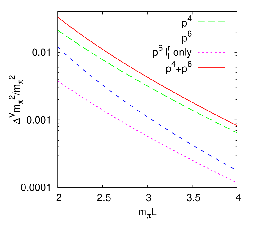
(a)

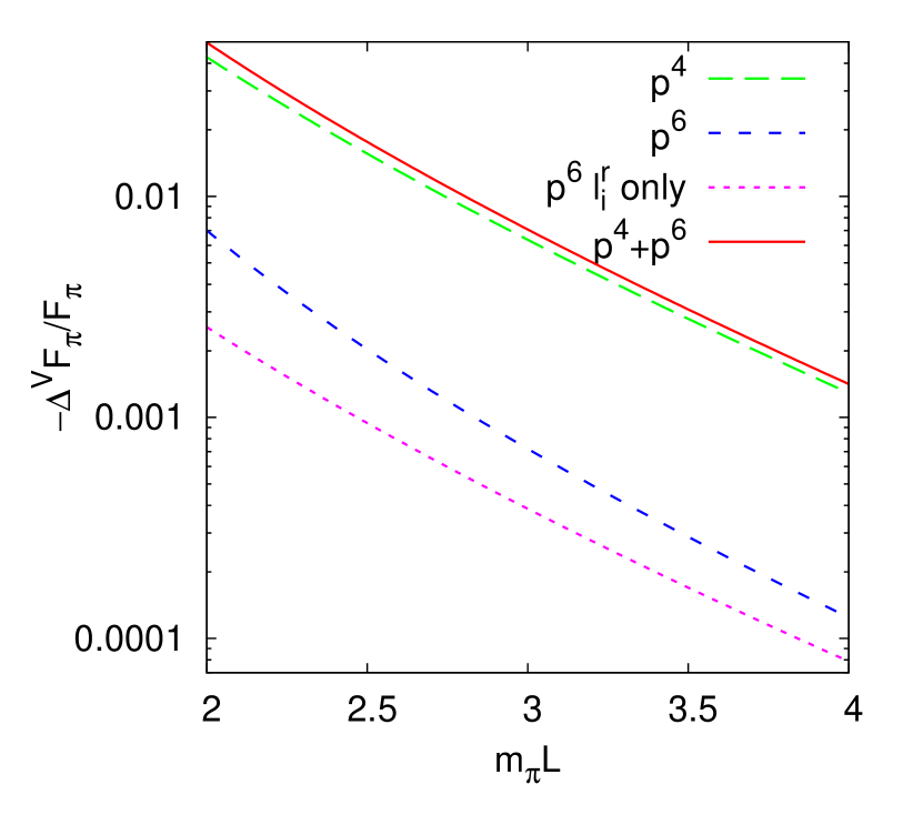
(b)

Figure 2: The relative finite volume corrections for the mass squared and decay constant of the pion in two-flavour ChPT at a fixed infinite volume pion mass $m_{\pi}=m_{\pi^{0}}$. Shown are the one-loop or $p^{4}$ corrections, the full $p^{6}$ result and the part only dependent on the $l_{i}^{r}$, $p^{6}l_{i}^{r}$, and the sum of the $p^{4}$ and $p^{6}$ result. $m_{\pi}L=2,4$ correspond to $L\approx 2.9,5.8$ fm. (a) The pion mass, plotted is $(m_{\pi}^{V2}-m_{\pi}^{2})/m_{\pi}^{2}$. (b) The pion decay constant. Plotted is $-(F_{\pi}^{V}-F_{\pi})/F_{\pi}$.

We can also perform a study of the corrections at other values of $m_{\pi}$ or as a function of $m_{\pi}$. One of the problems here is what to with the value of $F_{\pi}$ that should be used. If we use the infinite volume formulas to two-loop order of [24] which are expressed in the form $F_{\pi}/F=f(F_{\pi},m_{\pi})$ for another pion mass $\tilde{m}_{\pi}$ we determine the associated value of the decay constant, $\tilde{F}_{\pi}$ by solving $\tilde{F}_{\pi}/F_{\pi}=f(\tilde{F}_{\pi},\tilde{m}_{\pi})/f(F_{\pi},m_{\pi})$ numerically. The contribution from the $p^{6}$ LECs $c_{i}^{r}$ we have put to zero. This procedure might differ from the values of $\tilde{F}_{\pi}$ used in [12]. To compare with their numerical results we have plotted in Fig. 3 the equivalent of their Fig. 5. Namely $R_{m_{\pi}}=m_{\pi}^{V}/m_{\pi}-1$ where we have numerically calculated $R_{m_{\pi}}=\sqrt{(m_{\pi}^{2}+\Delta^{V}\!m_{\pi}^{2})/m_{\pi}^{2}}-1$. The calculated values of $F_{\pi}$ are $90.1,103.2,113.8$ for $m_{\pi}=100,300,500$ MeV. The resulting values of $R_{m_{\pi}}$ as shown in Fig. 3(a) are in reasonable agreement with Fig. 5 in [12]. There is already a difference at order $p^{4}$, so we suspect it is simply due to somewhat different values of $F_{\pi}$.

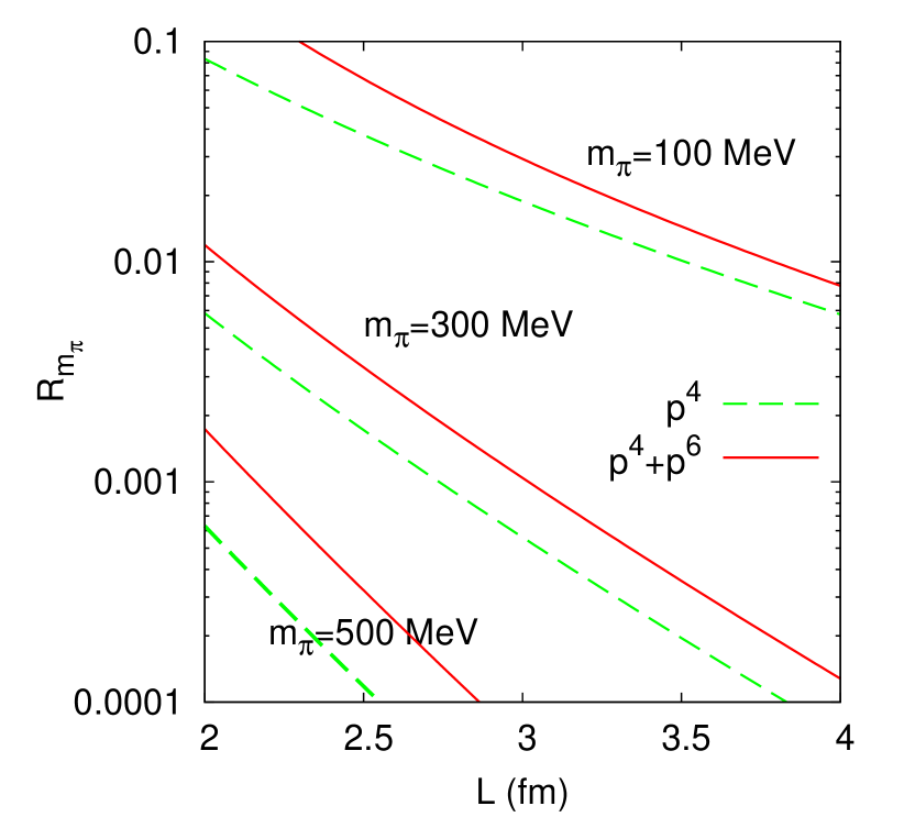
(a)

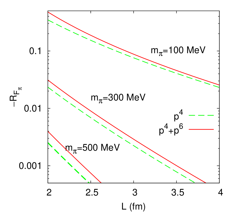
(b)

Figure 3: The relative finite volume corrections for the mass and decay constant of the pion in two-flavour ChPT at three values of the infinite volume pion mass. (a) $R_{m_{\pi}}=m_{\pi}^{V}/m_{\pi}-1$. (b) $R_{F_{\pi}}=F_{\pi}^{V}/F_{\pi}-1$, plotted is $-R_{F_{\pi}}$.

The one-loop result for $R_{F_{\pi}}$ agrees with Fig. 2 in [26] with small differences probably due to the difference in $F_{\pi}$ and the difference in the $l_{i}^{r}$-dependent part. Our result for the $p^{6}$ result is somewhat larger.

6.2 Three-flavour results: masses

The values of the low-energy constants, $L_{i}^{r}$ and $C_{i}^{r}$, we take from the review [31], in particular the set labeled BE14 there. In addition, the formulas require the infinite volume physical masses for the pion, kaon and eta mass as well as the pion decay constant. The masses and $F_{\pi}$ we use for the physical isospin averaged case are listed at the start of this section. For changed values of the infinite volume pion and kaon mass, $\tilde{m}_{\pi},\tilde{m}_{K}$, we proceed similarly to $F_{\pi}$ for the two-flavour case. We solve self-consistently the set of equations for $\tilde{m}_{\eta}$, $\tilde{F}_{\pi}$, $\tilde{F}_{K}/\tilde{F}_{\pi}$ and $\tilde{F}_{\eta}/\tilde{F}_{\pi}$. For the latter ratios we use the expanded version, similar to what was done in [31], see Eq. (45) in there. The results for a number of input cases is shown in Tab. 1.

$m_{\pi}$ $m_{K}$ $m_{\eta}$ $F_{\pi}$ $F_{K}/F_{\pi}$ $F_{\eta}/F_{\pi}$ $\hat{m}/\hat{m}_{\mathrm{phys}}$ $m_{s}/m_{s\mathrm{phys}}$ $m_{s}/\hat{m}$ 134.9764^∗ 494.53^∗ 545.9 92.2^∗ 1.199 1.306 1^∗ 1^∗ 27.3 100 487.14 540.46 90.4 1.219 1.337 0.547 1.000 49.9 300 549.6 593.73 101.4 1.099 1.154 5.025 1.000 5.43 100 400 446.53 87.3 1.199 1.293 0.518 0.644 33.9 100 495 549.07 90.7 1.219 1.340 0.550 1.037 51.4 300 495 533.00 100.3 1.094 1.138 4.867 0.778 4.36 495 495 495.00 108.0 1 1 12.70 0.465 1

Table 1: The self consistent solution for the infinite volume values of $m_{\eta}$, $F_{\pi}$, $F_{K}$, $F_{\eta}$ and the output quark mass ratios compared with the physical one. Units for dimensional quantities are in $MeV$. The input values for the physical case are starred.

The top line is the physical case The resulting output is within the expected quality of the fit in [31]. The next two lines have the kaon mass tuned to keep the same value of $m_{s}$. The value of $F_{\pi}$ can be compared with the result for the two-flavour case given above.

Let us have a look at the pion mass finite volume corrections for the physical case. The comparison of the two- and three-flavour results are plotted in Fig. 4(a). The one-loop result differs only by a very small kaon and eta loop. The difference is not visible in the figure. The two-loop results are also in very good agreement. The convergence is quite reasonable.

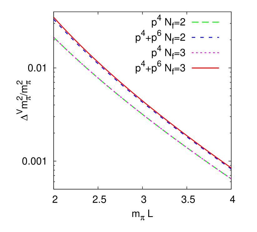
(a)

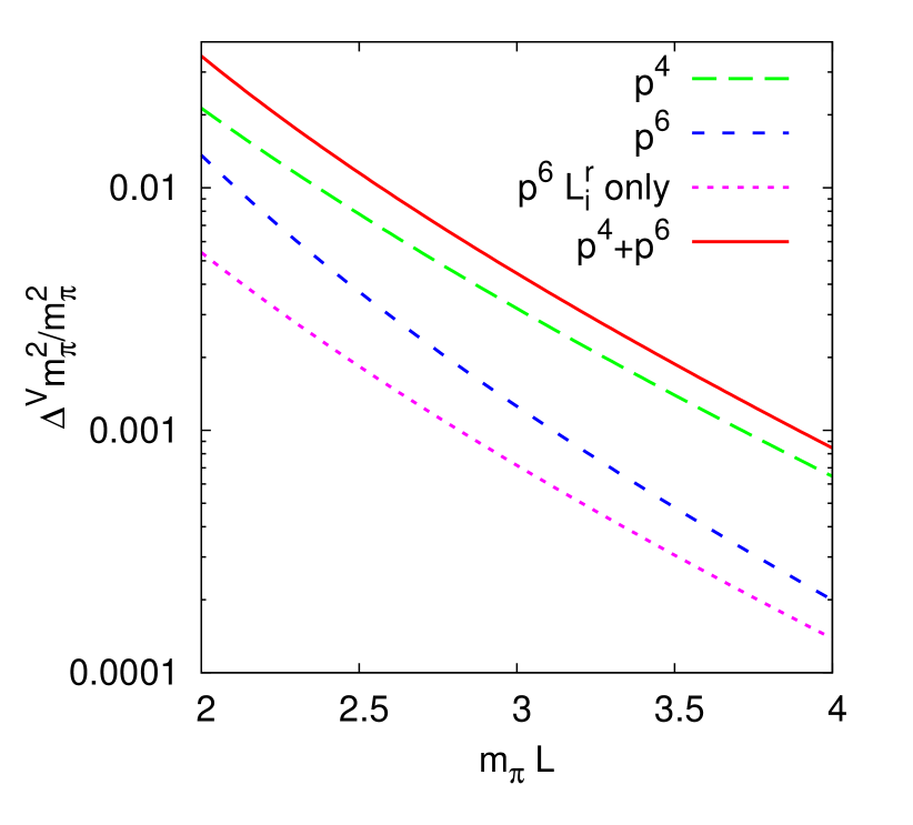
(b)

Figure 4: The finite volume corrections to the pion mass squared at $m_{\pi}=m_{\pi^{0}}$. All other inputs are given in the text. Plotted is the quantity $(m_{\pi}^{V2}-m_{\pi}^{2})/m_{\pi}^{2}$. (a) Comparison of the two- and three-flavour ChPT results. (b) The corrections for the three-flavour case also showing the $L_{i}^{r}$ dependent part.

The equivalent results for the kaon and eta are plotted in Fig. 5. The one-loop result for the kaon mass has only an eta loop as can be seen from (5). As a result, that part is very small. The total result is thus essentially coming only from two-loop order. The eta mass has a negative one-loop finite volume contribution. The pure loop part and the $L_{i}^{r}$-dependent part of the $p^{6}$ contribution are of the expected size. However, there is a very strong cancellation between the two parts leaving a very small positive correction. The total finite volume correction for the eta mass in negative.

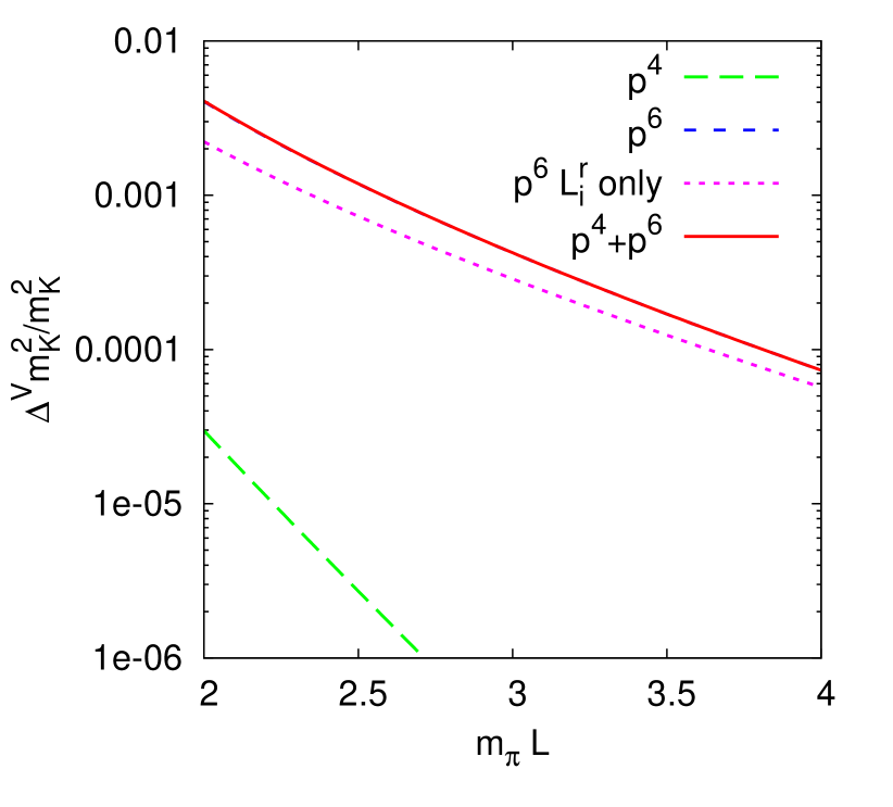
(a)

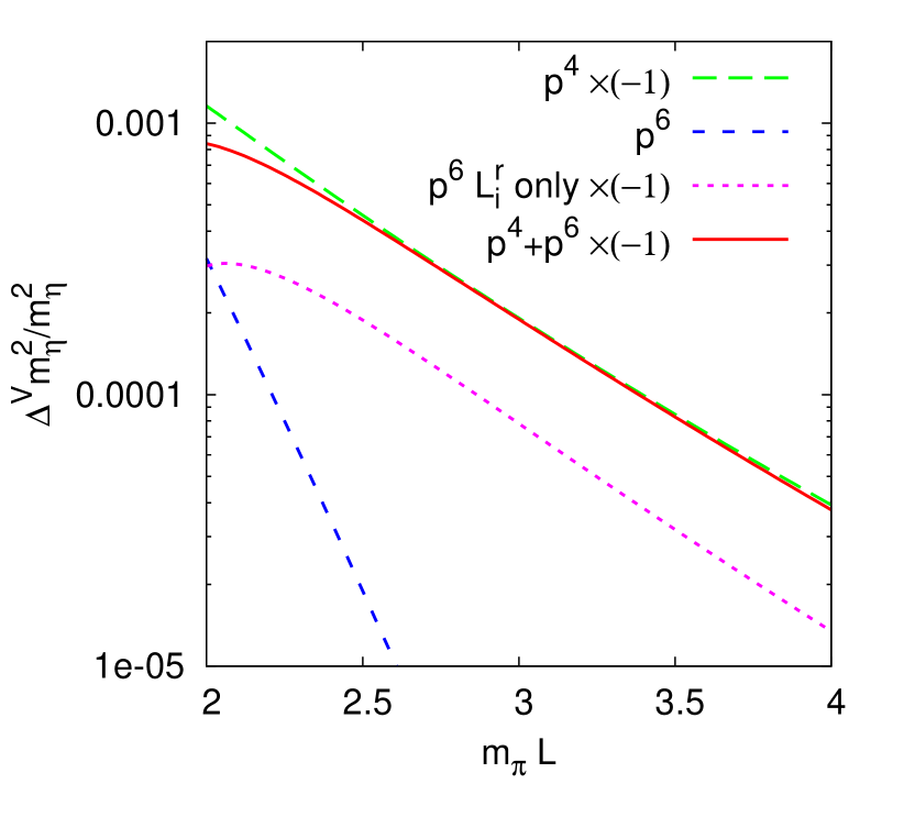
(b)

Figure 5: The corrections to the kaon and eta mass squared for the physical case. Plotted is the quantity $(m_{i}^{V2}-m_{i}^{2})/m_{i}^{2}$ for $i=K,\eta$. Shown are the one-loop, the two-loop, the sum and the two-loop $L_{i}^{r}$ dependent part. (a) Kaon, the $p^{4}$ is so small that $p^{6}$ and $p^{4}+p^{6}$ are indistinguishable. (b) Eta, note the signs, some parts are negative.

We can also check how the finite volume correction depends on the different masses. In Fig. 6 we have plotted the corrections to the pion mass squared for a number of different scenarios. In Fig. 6(a) we look at three cases. The bottom two lines are the physical case labeled with $m_{\pi}=m_{\pi^{0}}$ while the top four lines are with $m_{\pi}=100$ MeV. There we have plotted two cases, $m_{K}=400$ and $495$ MeV. The effect of the change in the pion mass is quite large while the effect due to the kaon mass change is smaller. The effect of changing the pion mass can be better seen in Fig. 6(b) where we kept the kaon mass at 495 MeV while varying the pion mass. The $L$ dependence is given as a function of $m_{\pi^{0}}L$ with the physical $\pi^{0}$ mass.

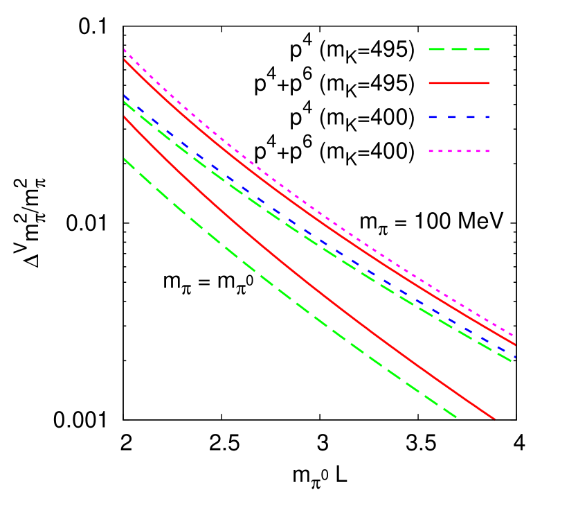
(a)

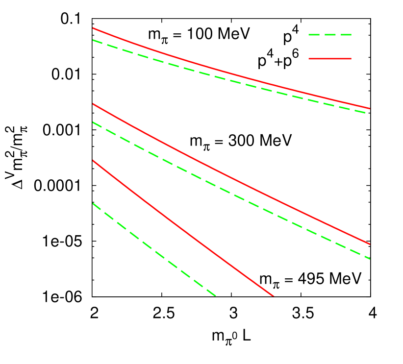
(b)

Figure 6: The finite volume corrections to the pion mass squared for a number of cases listed in Tab. 1. Plotted is the quantity $(m_{\pi}^{V2}-m_{\pi}^{2})/m_{\pi}^{2}$. (a) Physical case, bottom two lines, $(m_{\pi},m_{K})=(100,495)$ and $(100,400)$ MeV. (b) $m_{K}=495$ MeV and $m_{\pi}=100,300,495$ MeV. The size $L$ is given in units of the physical $\pi^{0}$ mass.

We have plotted the same cases for the finite volume corrections to the kaon mass squared in Fig. 7. The one-loop correction for the physical case and $m_{\pi},m_{K}=100,495$ MeV is virtually identical. The $p^{4}+p^{6}$ is a bit more different for the three cases as can be seen in Fig. 7(a). In Fig. 7(b) we have shown the corrections for a fixed kaon mass but three different pion masses. The bottom three lines are the one-loop result while the top three lines are the full result. Note that, as it should be, the case where the pion mass and kaon mass are the same, the finite volume corrections to the kaon are the same as for the pion in Fig. 6(b). This is another small check on our result.

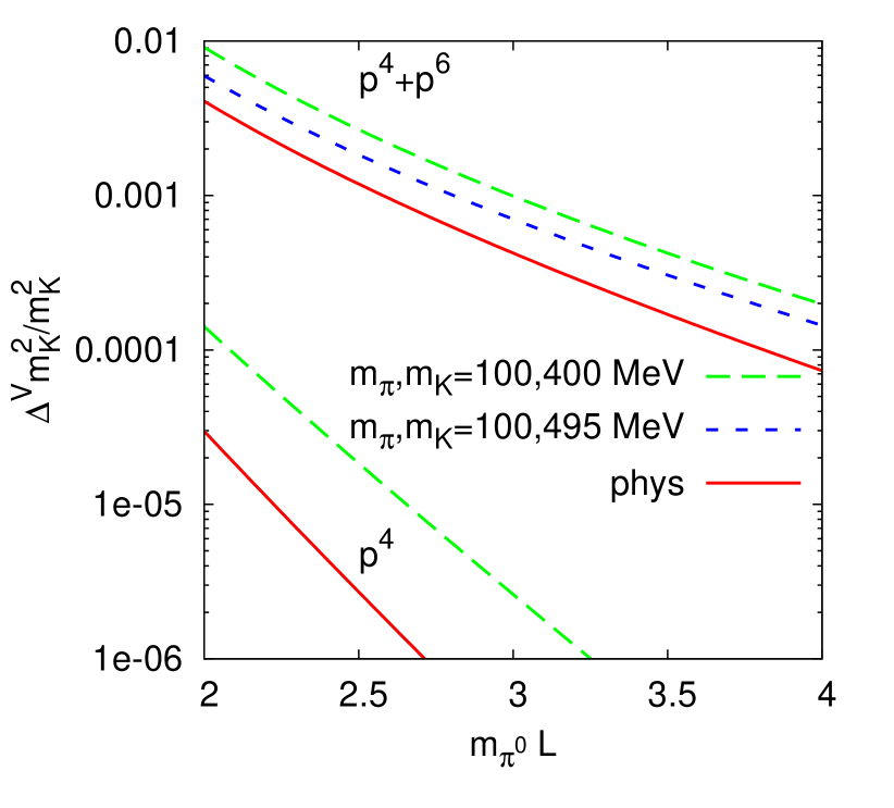
(a)

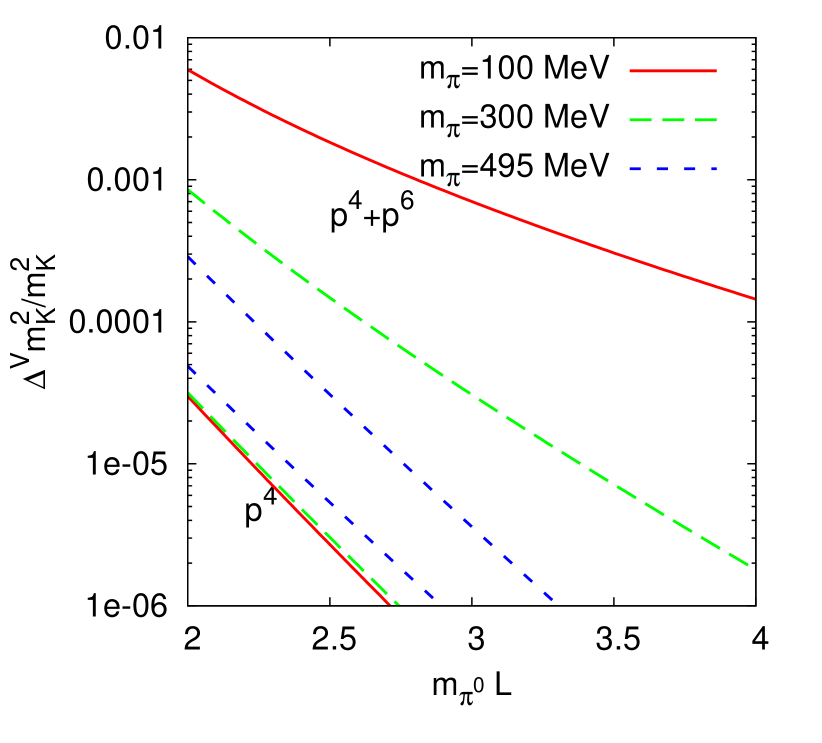
(b)

Figure 7: The finite volume corrections to the kaon mass squared for a number of cases listed in Tab. 1.for the physical case. Plotted is the quantity $(m_{K}^{V2}-m_{K}^{2})/m_{K}^{2}$. (a) Physical case and $(m_{\pi},m_{K})=(100,495)$ and $(100,400)$ MeV. (b) $m_{K}=495$ MeV and $m_{\pi}=100,300,495$ MeV. The size $L$ is given in units of the physical $\pi^{0}$ mass.

We have plotted the same cases once more for the finite volume corrections to the eta mass squared in Fig. 8. Here the result is rather variable due to cancellations. In Fig. 8(a) the one-loop corrections increase going from the physical case via $m_{\pi},m_{K}=100,495$ MeV to $m_{\pi},m_{K}=100,400$ MeV. The two-loop corrections are rather small in the first two cases, due to the cancellations between the pure two-loop and the $L_{i}^{r}$ dependent part. The one-loop correction for the physical case and $m_{\pi},m_{K}=100,495$ MeV is virtually identical. The $p^{4}+p^{6}$ is a bit more different for the three cases. In Fig. 8(b) we have shown the corrections for a fixed kaon mass but three different pion masses. The bottom lines are the case with $m_{\pi},m_{K}=495$ MeV. It agrees with the pion and kaon corrections for this case. For $m_{\pi}=300$ MeV the correction is negative but goes through zero for small $L$ due to a cancellation between one-and two-loop results. The $p^{6}$ correction for $m_{\pi}=100$ MeV is very small, we again have a large cancellation between the pure two-loop and the $L_{i}^{r}$ dependent part.

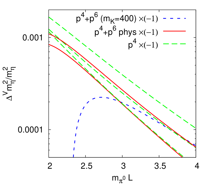
(a)

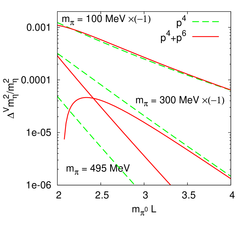
(b)

Figure 8: The finite volume corrections to the eta mass squared for a number of cases listed in Tab. 1.for the physical case. Plotted is the quantity $(m_{\eta}^{V2}-m_{\eta}^{2})/m_{\eta}^{2}$. (a) Physical case and $(m_{\pi},m_{K})=(100,495)$ and $(100,400)$ MeV. Lines are for the one-loop result at the right bottom physical case, middle $(m_{\pi},m_{K})=(100,495)$, top $(m_{\pi},m_{K})=(100,400)$. The first two have only a small change due to $p^{6}$, while for the last case there is a large cancellation between one and two-loops. (b) $m_{K}=495$ MeV and $m_{\pi}=100,300,495$ MeV. The size $L$ is given in units of the physical $\pi^{0}$ mass.

We did not compare with the numerical results in [27], since there was a small mistake in the relevant figures [32].

6.3 Three-flavour results: decay constants

We will use exactly the same input values as in the previous subsection now but for the decay constants. Note that here in most cases the finite volume correction is negative.

The comparison of the two- and three-flavour results for the pion decay constant is plotted in Fig. 9(a). The one-loop result differs only by a very small kaon and eta loop. The difference is not visible in the figure. The two-loop results are also essentially indistinguishable. The convergence is quite reasonable. The bottom line and top line(s) are respectively the one-loop and the sum of one- and two-loops. Note that in agreement with the earlier estimates there is a sizable correction at finite volume even at $m_{\pi}L=2$.

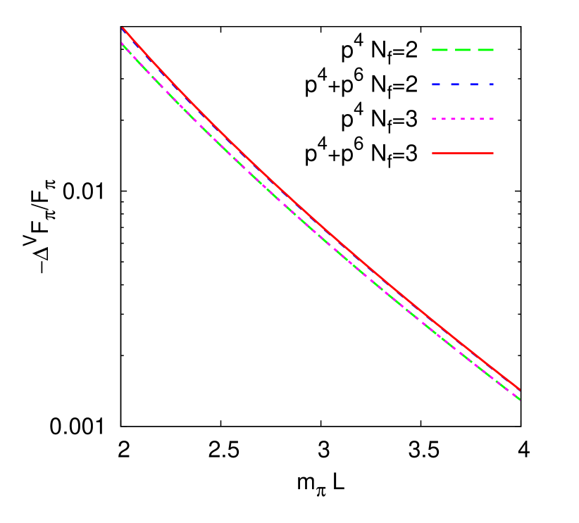
(a)

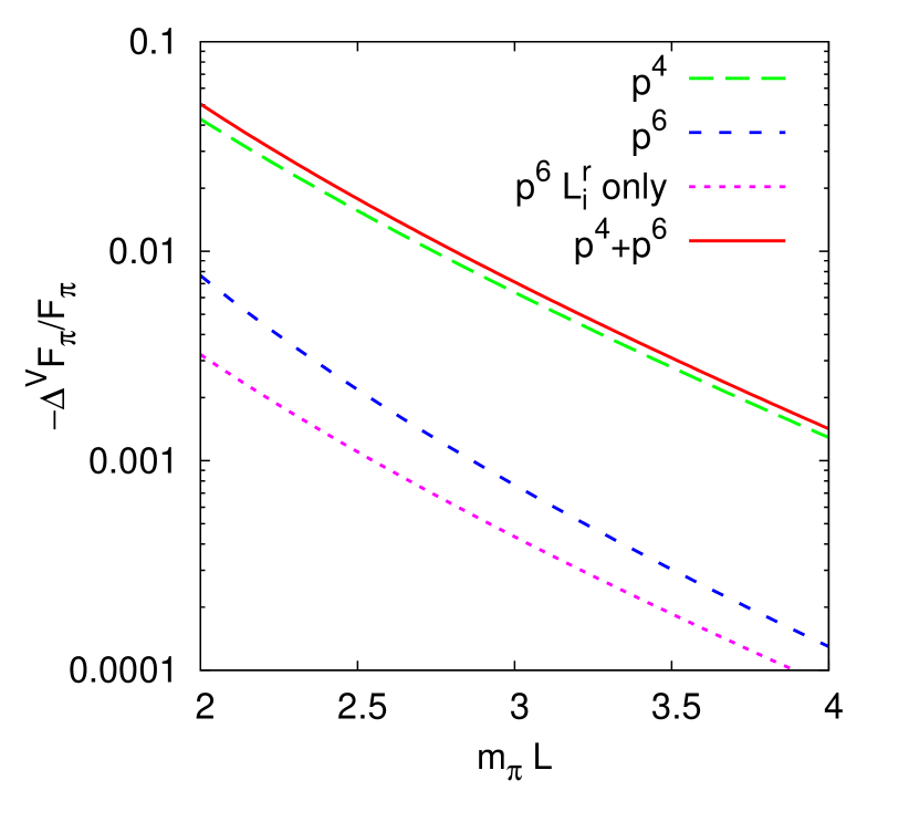
(b)

Figure 9: The finite volume corrections to the pion decay constant at $m_{\pi}=m_{\pi^{0}}$. All other inputs are given in the text. Plotted is the quantity $-(F_{\pi}^{V}-F_{\pi})/F_{\pi}$. (a) Comparison of the two- and three-flavour ChPT results. (b) The corrections for the three-flavour case also showing the $L_{i}^{r}$ dependent part.

The equivalent results for the kaon and eta are plotted in Fig. 10. The kaon decay constant corrections are somewhat smaller than for the pion, but still important for precision studies. The one-loop result for the eta decay constant has only a kaon loop as can be seen from (5). As a result, that part is very small. The total result comes mainly from two-loop order. The eta mass has a negative one-loop finite volume contribution. The pure loop part and the $L_{i}^{r}$-dependent part of the $p^{6}$ contribution are of the expected size. However, there is a very strong cancellation between the two parts leaving a very small positive correction. The total finite volume correction for the eta decay constant is quite small.

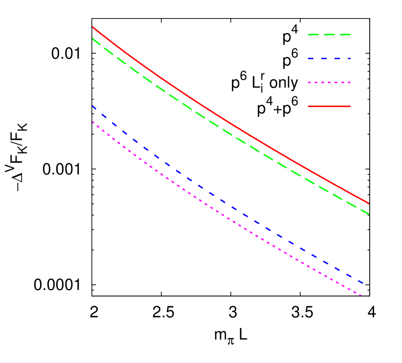
(a)

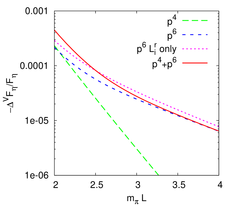
(b)

Figure 10: The corrections to the kaon and eta decay constant for the physical case. Plotted is the quantity $-(F_{i}^{V}-F_{i})/F_{i}$ for $i=K,\eta$. Shown are the one-loop, the two-loop, the sum and the two-loop $L_{i}^{r}$ dependent part. (a) Kaon. (b) Eta.

We can also check how the finite volume correction depends on the different masses. In Fig. 6 we have plotted the corrections to the pion decay constant for several scenarios. In Fig. 11(a) we look at three cases. The bottom two lines are the physical case labeled with $m_{\pi}=m_{\pi^{0}}$ while the top four lines are with $m_{\pi}=100$ MeV. There we have plotted two cases, $m_{K}=400$ and $495$ MeV. The effect of the change in the pion mass is quite large while the effect due to the kaon mass change is smaller. In Fig. 11(b) we can see the effect of only varying the pion mass.

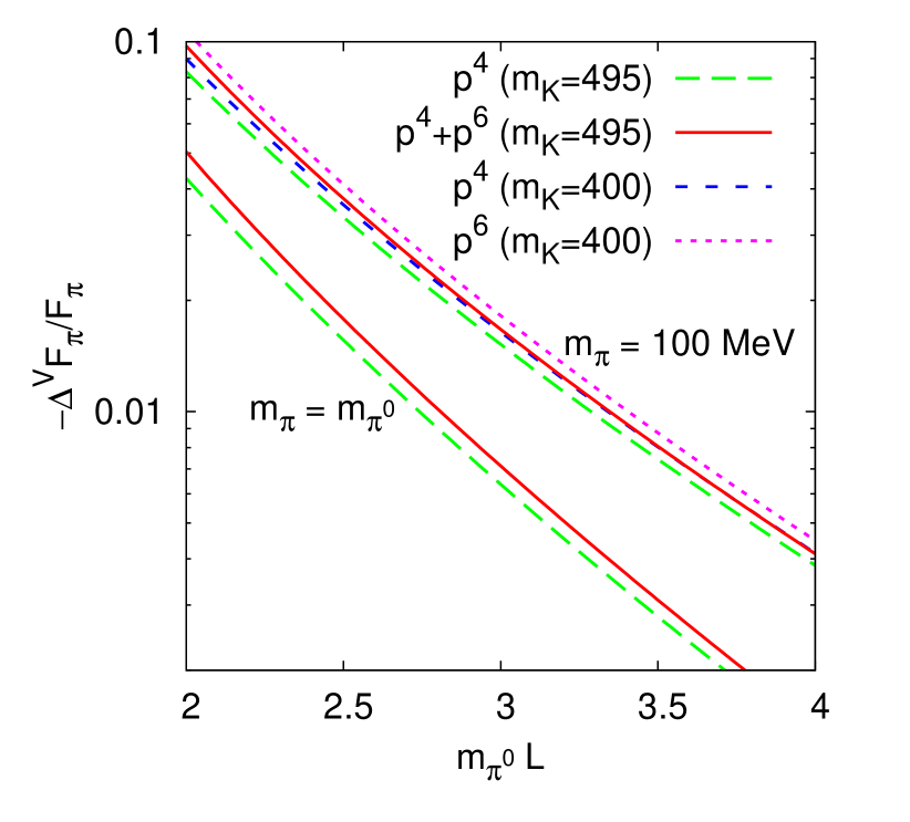
(a)

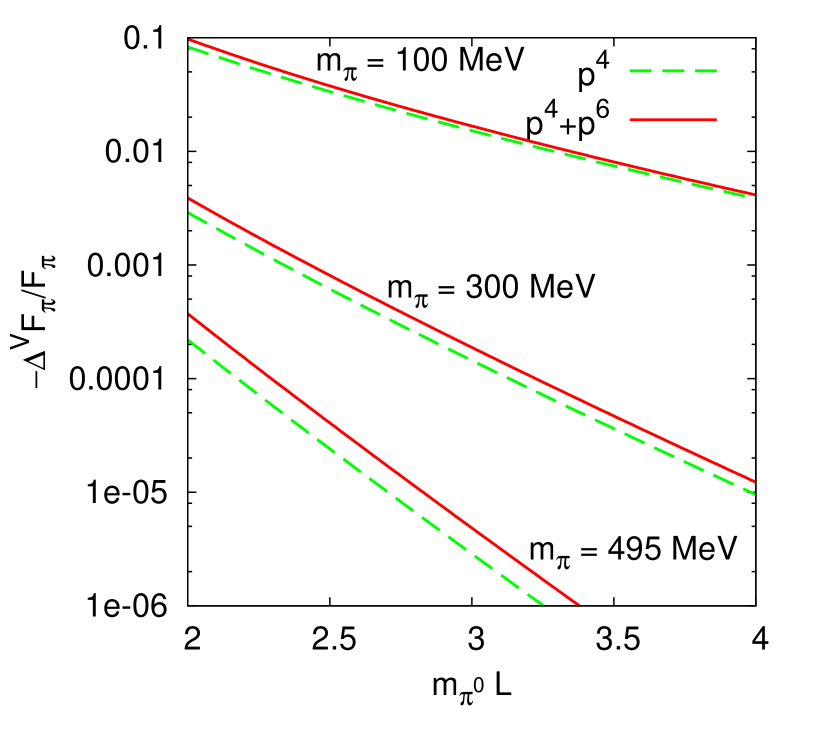
(b)

Figure 11: The finite volume corrections to the pion decay constant for a number of cases listed in Tab. 1. Plotted is the quantity $-(F_{\pi}^{V}-F_{\pi})/F_{\pi}$. (a) Physical case and $(m_{\pi},m_{K})=(100,495)$ and $(100,400)$ MeV. (b) $m_{K}=495$ MeV and $m_{\pi}=100,300,495$ MeV. The size $L$ is given in units of the physical $\pi^{0}$ mass.

We have plotted the same cases for the finite volume corrections to the kaon decay constant in Fig. 12. In Fig. 12(a), the bottom two-lines are the physical case. The four top lines are with $m_{\pi}=100$ MeV, where the smaller kaon mass gives a somewhat larger correction. In Fig. 12(b) we have shown the corrections for a fixed kaon mass but three different pion masses. The bottom three lines are the one-loop result while the top three lines are the full result. Note that, as it should be, for the case where the pion mass and kaon mass are the same, the finite volume corrections to the kaon are the same as for the pion in Fig. 11(b). This is another small check on our result.

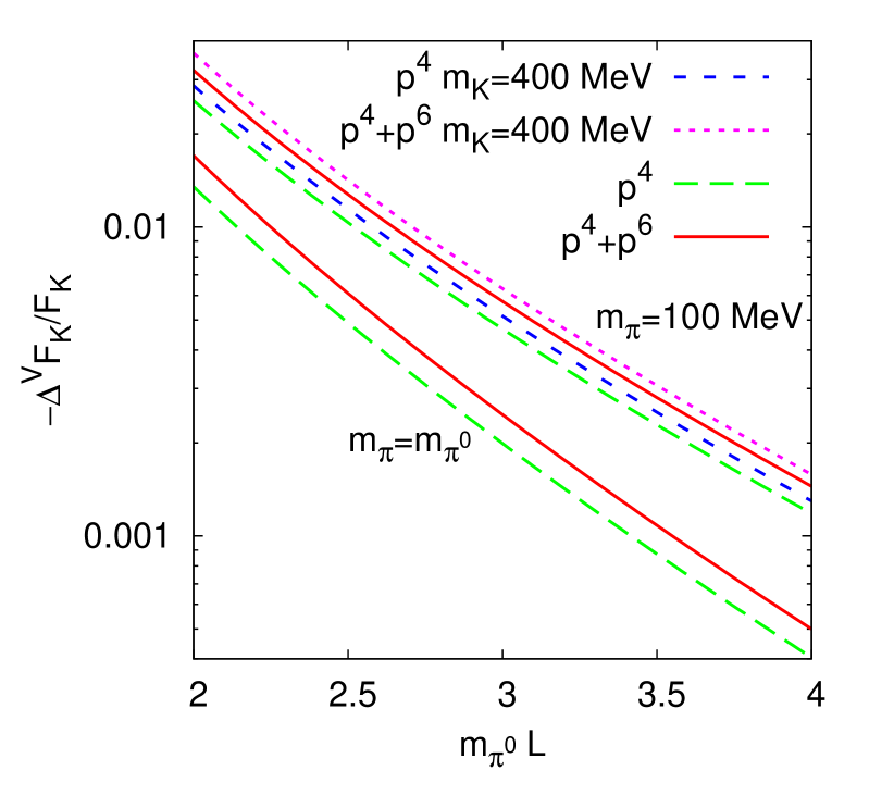
(a)

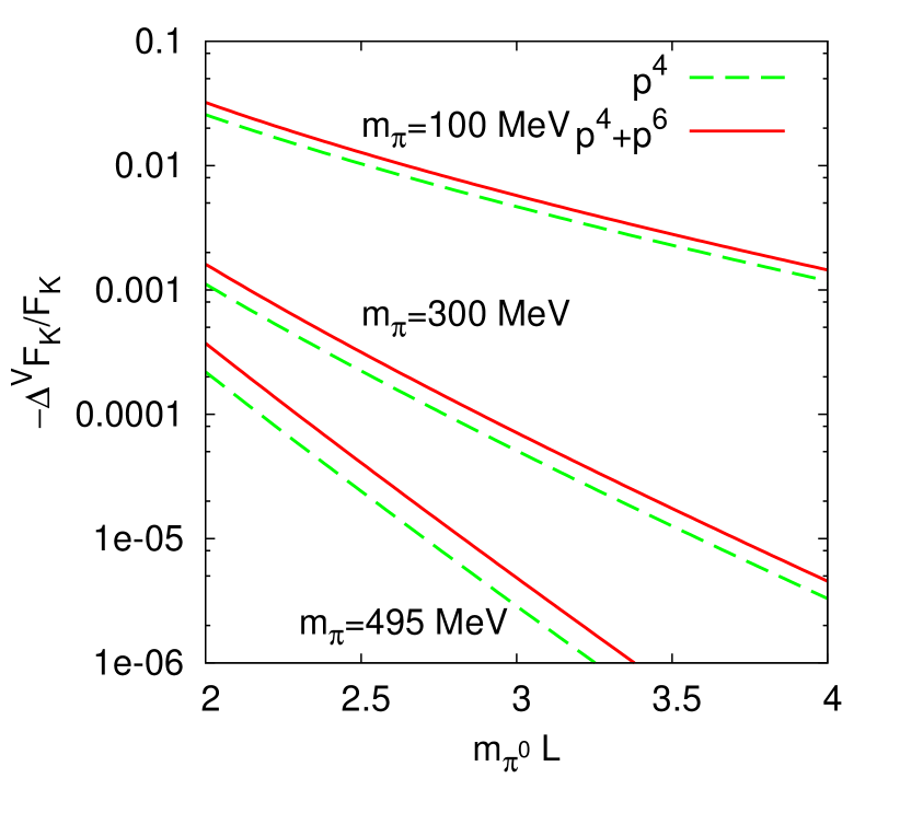
(b)

Figure 12: The finite volume corrections to the kaon decay constant for a number of cases listed in Tab. 1. Plotted is the quantity $-(F_{K}^{V}-F_{K})/F_{K}$. (a) Physical case and $(m_{\pi},m_{K})=(100,495)$ and $(100,400)$ MeV. (b) $m_{K}=495$ MeV and $m_{\pi}=100,300,495$ MeV. The size $L$ is given in units of the physical $\pi^{0}$ mass.

We have plotted the same cases once more for the finite volume corrections to the eta decay constant squared in Fig. 13. In Fig. 13(a) the one-loop corrections for the physical case and $m_{\pi},m_{K}=100,495$ MeV are extremely close, since it only depends on the kaon mass. The $p^{6}$ corrections for both cases are quite different though. Finally, for $m_{\pi},m_{K}=100,400$ MeV both the one- and two-loop corrections are larger but the total correction remains fairly small. In Fig. 13(b) we have shown the corrections for a fixed kaon mass but three different pion masses. The $p^{4}$ correction is thus identical for the three cases. The correction for $m_{\pi},m_{K}=495$ MeV agrees with the pion and kaon corrections for this case. The total correction remains small for all cases.

(a)

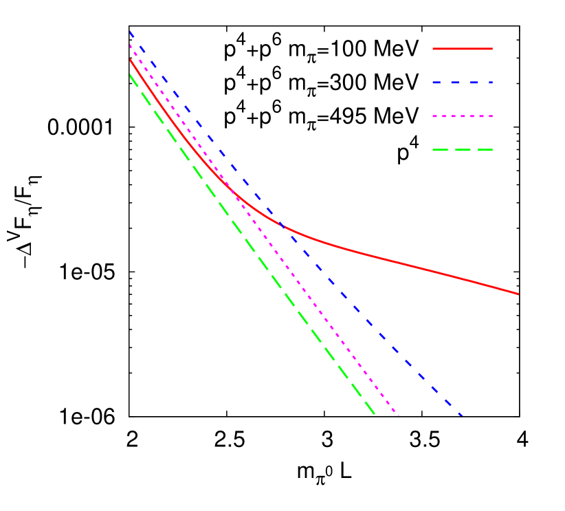
(b)

Figure 13: The finite volume corrections to the eta decay constant for a number of cases listed in Tab. 1. Plotted is the quantity $-(F_{\eta}^{V}-F_{\eta})/F_{\eta}$. (a) Physical case and $(m_{\pi},m_{K})=(100,495)$ and $(100,400)$ MeV. The bottom line is the one-loop result for the physical case and $(m_{\pi},m_{K})=(100,495)$. Others as labeled. (b) $m_{K}=495$ MeV and $m_{\pi}=100,300,495$ MeV. The size $L$ is given in units of the physical $\pi^{0}$ mass.

We did not compare with the numerical results in [27], since there was a small mistake in the relevant figures [32].

7 Conclusions

In this paper we calculated the finite volume corrections to two-loop order in ChPT. The pion mass and decay constant we calculated both in two and three-flavour ChPT. The kaon and eta mass and decay constant we obtained in three-flavour ChPT. These expressions in the main text and the appendices are the main result of this work.

We have compared as far as possible with existing work, where we are in agreement with the known one-loop results and have some disagreements with the existing results at two-loop order. What we agree on and differ on is discussed in Sects. 4 and 5. Note that a full comparison at the analytical level was not possible due to the large differences in the loop integral treatments.

We have presented numerical results for a number of representative cases. In all cases the exponential decay $e^{-m_{\pi}/L}$ is clearly visible and as expected the numbers are dominated by the finite volume pion loops. The corrections at order $p^{6}$ are sometimes large, especially when the order $p^{4}$ result did not contain pion loops. We find that the finite volume corrections are necessary for the pion mass and decay constant as well as the kaon decay constant. The kaon mass receives corrections at a somewhat lower level while finite volume corrections for the eta mass and decay constant are at present negligible.

The numerical work has been done using C++. The programs will be made available together with the infinite volume results in [33]. The analytical work relied heavily on FORM [34].

Appendix A Three flavour $p^{6}$ expressions for the masses

This appendix lists the order $p^{6}$ result for the three-flavour ChPT finite volume corrections to the masses squared at order $p^{6}$.

$$F_{\pi}^{4}\Delta^{V}\!m^{2(6)}_{\pi}={A}^{V}(m_{\pi}^{2})m_{\pi}^{4}\,\Big{(}40\,L^{r}_{8}+80\,L^{r}_{6}-24\,L^{r}_{5}-48\,L^{r}_{4}+28\,L^{r}_{3}+32\,L^{r}_{2}+56\,L^{r}_{1}\Big{)}$$ (20)

$$+{A}^{V}(m_{K}^{2})m_{\pi}^{2}\,m_{K}^{2}\,\Big{(}32\,L^{r}_{8}+64\,L^{r}_{6}-16\,L^{r}_{5}-64\,L^{r}_{4}+20\,L^{r}_{3}+16\,L^{r}_{2}+64\,L^{r}_{1}\Big{)}$$

$$+{A}^{V}(m_{\eta}^{2})m_{\pi}^{2}\,\Big{(}8\,L^{r}_{8}m_{\pi}^{2}-64/3\,L^{r}_{7}\,m_{K}^{2}+64/3\,L^{r}_{7}m_{\pi}^{2}+64/3\,L^{r}_{6}\,m_{K}^{2}-16/3\,L^{r}_{6}m_{\pi}^{2}$$

$$-32/9\,L^{r}_{5}m_{K}^{2}+8/9\,L^{r}_{5}m_{\pi}^{2}-64/3\,L^{r}_{4}m_{K}^{2}+16/3\,L^{r}_{4}m_{\pi}^{2}+16/3\,L^{r}_{3}m_{K}^{2}-4/3\,L^{r}_{3}$$

$$m_{\pi}^{2}+16/3\,L^{r}_{2}m_{K}^{2}-4/3\,L^{r}_{2}m_{\pi}^{2}+64/3\,L^{r}_{1}m_{K}^{2}-16/3\,L^{r}_{1}m_{\pi}^{2}\Big{)}$$

$$+{A}_{23}^{V}(m_{\pi}^{2})m_{\pi}^{2}\,\Big{(}-12\,L^{r}_{3}-48\,L^{r}_{2}-24\,L^{r}_{1}\Big{)}+{A}_{23}^{V}(m_{K}^{2})m_{\pi}^{2}\,\Big{(}-12\,L^{r}_{3}-48\,L^{r}_{2}\Big{)}$$

$$+{A}_{23}^{V}(m_{\eta}^{2})m_{\pi}^{2}\,\Big{(}-4\,L^{r}_{3}-12\,L^{r}_{2}\Big{)}$$

$$+{A}^{V}(m_{\pi}^{2})m_{\pi}^{2}\,\Big{(}\frac{1}{16\pi^{2}}\,m_{K}^{2}+3/4\,\frac{1}{16\pi^{2}}\,m_{\pi}^{2}-7/4\,\overline{A}(m_{\pi}^{2})-\overline{A}(m_{K}^{2})+1/12\,\overline{B}^{0}(m_{\eta}^{2})\,m_{\pi}^{2}\Big{)}$$

$$+{A}^{V}(m_{\pi}^{2})^{2}\,\Big{(}-3/8\,m_{\pi}^{2}\Big{)}+{A}^{V}(m_{\pi}^{2})\,{A}^{V}(m_{K}^{2})\,\Big{(}-1/2\,m_{\pi}^{2}\Big{)}$$

$$+{A}^{V}(m_{\pi}^{2})\,{A}^{V}(m_{\eta}^{2})\,\Big{(}-1/12\,m_{\pi}^{2}\Big{)}+{A}^{V}(m_{\pi}^{2})\,{B}^{0V}(m_{\pi}^{2})\,\Big{(}1/4\,m_{\pi}^{4}\Big{)}$$

$$+{A}^{V}(m_{\pi}^{2})\,{B}^{0V}(m_{\eta}^{2})\,\Big{(}1/12\,m_{\pi}^{4}\Big{)}$$

$$+{A}^{V}(m_{K}^{2})m_{\pi}^{2}\,\Big{(}\frac{1}{16\pi^{2}}m_{K}^{2}-1/2\,\overline{A}(m_{\pi}^{2})-1/2\,\overline{A}(m_{K}^{2})-1/2\,\overline{A}(m_{\eta}^{2})-2/9\,\overline{B}^{0}(m_{\eta}^{2})\,m_{K}^{2}\Big{)}$$

$$+{A}^{V}(m_{K}^{2})^{2}\,\Big{(}-1/4\,m_{\pi}^{2}\Big{)}+{A}^{V}(m_{K}^{2})\,{A}^{V}(m_{\eta}^{2})\,\Big{(}-1/2\,m_{\pi}^{2}\Big{)}+{A}^{V}(m_{K}^{2})\,{B}^{0V}(m_{\eta}^{2})\,\Big{(}-2/9\,m_{\pi}^{2}\,m_{K}^{2}\Big{)}$$

$$+{A}^{V}(m_{\eta}^{2})m_{\pi}^{2}\,\Big{(}1/12\,\frac{1}{16\pi^{2}}\,m_{\pi}^{2}+1/4\,\overline{A}(m_{\pi}^{2})-1/3\,\overline{A}(m_{K}^{2})+\,\overline{B}^{0}(m_{\eta}^{2})\left(4/27\,m_{K}^{2}-7/108\,m_{\pi}^{2}\right)\Big{)}$$

$$+{A}^{V}(m_{\eta}^{2})^{2}\,\Big{(}1/72\,m_{\pi}^{2}\Big{)}+{A}^{V}(m_{\eta}^{2})\,{B}^{0V}(m_{\pi}^{2})\,\Big{(}-1/12\,m_{\pi}^{4}\Big{)}$$

$$+{A}^{V}(m_{\eta}^{2})\,{B}^{0V}(m_{\eta}^{2})\,\Big{(}4/27\,m_{\pi}^{2}\,m_{K}^{2}-7/108\,m_{\pi}^{4}\Big{)}$$

$$+{H}^{V}(m_{\pi}^{2},m_{\pi}^{2},m_{\pi}^{2},m_{\pi}^{2})\,\Big{(}5/6\,m_{\pi}^{4}\Big{)}+{H}^{V}(m_{\pi}^{2},m_{K}^{2},m_{K}^{2},m_{\pi}^{2})\,\Big{(}m_{\pi}^{2}\,m_{K}^{2}-5/8\,m_{\pi}^{4}\Big{)}$$

$$+{H}^{V}(m_{\pi}^{2},m_{\eta}^{2},m_{\eta}^{2},m_{\pi}^{2})\,\Big{(}1/18\,m_{\pi}^{4}\Big{)}+{H}^{V}(m_{K}^{2},m_{K}^{2},m_{\eta}^{2},m_{\pi}^{2})\,\Big{(}1/2\,m_{\pi}^{2}\,m_{K}^{2}+1/24\,m_{\pi}^{4}\Big{)}$$

$$+{H}_{1}^{V}(m_{\pi}^{2},m_{K}^{2},m_{K}^{2},m_{\pi}^{2})\,\Big{(}m_{\pi}^{4}\Big{)}+{H}_{1}^{V}(m_{\eta}^{2},m_{K}^{2},m_{K}^{2},m_{\pi}^{2})\,\Big{(}-m_{\pi}^{4}\Big{)}$$

$$+{H}_{21}^{V}(m_{\pi}^{2},m_{\pi}^{2},m_{\pi}^{2},m_{\pi}^{2})\,\Big{(}3\,m_{\pi}^{4}\Big{)}+{H}_{21}^{V}(m_{\pi}^{2},m_{K}^{2},m_{K}^{2},m_{\pi}^{2})\,\Big{(}-3/8\,m_{\pi}^{4}\Big{)}$$

$$+{H}_{21}^{V}(m_{K}^{2},m_{\pi}^{2},m_{K}^{2},m_{\pi}^{2})\,\Big{(}3\,m_{\pi}^{4}\Big{)}+{H}_{21}^{V}(m_{\eta}^{2},m_{K}^{2},m_{K}^{2},m_{\pi}^{2})\,\Big{(}9/8\,m_{\pi}^{4}\Big{)}$$

$$+{H}_{27}^{V}(m_{\pi}^{2},m_{\pi}^{2},m_{\pi}^{2},m_{\pi}^{2})\,\Big{(}-3\,m_{\pi}^{2}\Big{)}+{H}_{27}^{V}(m_{\pi}^{2},m_{K}^{2},m_{K}^{2},m_{\pi}^{2})\,\Big{(}3/8\,m_{\pi}^{2}\Big{)}$$

$$+{H}_{27}^{V}(m_{K}^{2},m_{\pi}^{2},m_{K}^{2},m_{\pi}^{2})\,\Big{(}-3\,m_{\pi}^{2}\Big{)}+{H}_{27}^{V}(m_{\eta}^{2},m_{K}^{2},m_{K}^{2},m_{\pi}^{2})\,\Big{(}-9/8\,m_{\pi}^{2}\Big{)}\,.$$

$$F_{\pi}^{4}\Delta^{V}\!m^{2(6)}_{K}={A}^{V}(m_{\pi}^{2})\,\Big{(}24\,L^{r}_{8}m_{\pi}^{2}\,m_{K}^{2}+48\,L^{r}_{6}m_{\pi}^{2}\,m_{K}^{2}-12\,L^{r}_{5}m_{\pi}^{2}\,m_{K}^{2}-48\,L^{r}_{4}m_{\pi}^{2}\,m_{K}^{2}$$ (21)

$$+15\,L^{r}_{3}m_{\pi}^{2}\,m_{K}^{2}+12\,L^{r}_{2}m_{\pi}^{2}\,m_{K}^{2}+48\,L^{r}_{1}m_{\pi}^{2}\,m_{K}^{2}\Big{)}$$

$$+{A}^{V}(m_{K}^{2})\,\Big{(}48\,L^{r}_{8}m_{K}^{4}+96\,L^{r}_{6}m_{K}^{4}-24\,L^{r}_{5}m_{K}^{4}-64\,L^{r}_{4}\,m_{K}^{4}+30\,L^{r}_{3}m_{K}^{4}+36\,L^{r}_{2}m_{K}^{4}+72\,L^{r}_{1}m_{K}^{4}\Big{)}$$

$$+{A}^{V}(m_{\eta}^{2})\,\Big{(}64/3\,L^{r}_{8}m_{K}^{4}-56/3\,L^{r}_{8}m_{\pi}^{2}\,m_{K}^{2}+16/3\,L^{r}_{8}m_{\pi}^{4}+64/3\,L^{r}_{7}m_{K}^{4}-32\,L^{r}_{7}m_{\pi}^{2}\,m_{K}^{2}$$

$$+32/3\,L^{r}_{7}m_{\pi}^{4}+64/3\,L^{r}_{6}m_{K}^{4}-16/3\,L^{r}_{6}m_{\pi}^{2}\,m_{K}^{2}-64/9\,L^{r}_{5}m_{K}^{4}+4/3\,L^{r}_{5}m_{\pi}^{2}\,m_{K}^{2}-8/9\,L^{r}_{5}m_{\pi}^{4}$$

$$-64/3\,L^{r}_{4}m_{K}^{4}+16/3\,L^{r}_{4}m_{\pi}^{2}\,m_{K}^{2}+28/3\,L^{r}_{3}m_{K}^{4}-7/3\,L^{r}_{3}m_{\pi}^{2}\,m_{K}^{2}+16/3\,L^{r}_{2}m_{K}^{4}$$

$$-4/3\,L^{r}_{2}m_{\pi}^{2}\,m_{K}^{2}+64/3\,L^{r}_{1}m_{K}^{4}-16/3\,L^{r}_{1}m_{\pi}^{2}\,m_{K}^{2}\Big{)}$$

$$+{A}_{23}^{V}(m_{\pi}^{2})\,\Big{(}-9\,L^{r}_{3}m_{K}^{2}-36\,L^{r}_{2}m_{K}^{2}\Big{)}+{A}_{23}^{V}(m_{K}^{2})\,\Big{(}-18\,L^{r}_{3}m_{K}^{2}-60\,L^{r}_{2}m_{K}^{2}-24\,L^{r}_{1}m_{K}^{2}\Big{)}$$

$$+{A}_{23}^{V}(m_{\eta}^{2})\,\Big{(}-L^{r}_{3}m_{K}^{2}-12\,L^{r}_{2}m_{K}^{2}\Big{)}$$

$$+{A}^{V}(m_{\pi}^{2})\,\Big{(}3/4\,\frac{1}{16\pi^{2}}\,m_{K}^{4}-3/16\,\overline{A}(m_{\pi}^{2})\,m_{K}^{2}-3/4\,\overline{A}(m_{K}^{2})\,m_{K}^{2}-3/16\,\overline{A}(m_{\eta}^{2})\,m_{K}^{2}$$

$$-1/6\,\overline{B}^{0}(m_{\eta}^{2})\,m_{\pi}^{2}\,m_{K}^{2}\Big{)}$$

$$+{A}^{V}(m_{\pi}^{2})^{2}\,\Big{(}-3/32\,m_{K}^{2}\Big{)}+{A}^{V}(m_{\pi}^{2})\,{A}^{V}(m_{K}^{2})\,\Big{(}-3/4\,m_{K}^{2}\Big{)}+{A}^{V}(m_{\pi}^{2})\,{A}^{V}(m_{\eta}^{2})\,\Big{(}-3/16\,m_{K}^{2}\Big{)}$$

$$+{A}^{V}(m_{\pi}^{2})\,{B}^{0V}(m_{\eta}^{2})\,\Big{(}-1/6\,m_{\pi}^{2}\,m_{K}^{2}\Big{)}$$

$$+{A}^{V}(m_{K}^{2})\,\Big{(}3/4\,\frac{1}{16\pi^{2}}\,m_{K}^{4}+3/4\,\frac{1}{16\pi^{2}}\,m_{\pi}^{2}\,m_{K}^{2}-3/4\,\overline{A}(m_{\pi}^{2})\,m_{K}^{2}-3/2\,\overline{A}(m_{K}^{2})\,m_{K}^{2}$$

$$+4/9\,\overline{B}^{0}(m_{\eta}^{2})\,m_{K}^{4}\Big{)}$$

$$+{A}^{V}(m_{K}^{2})^{2}\,\Big{(}-3/4\,m_{K}^{2}\Big{)}+{A}^{V}(m_{K}^{2})\,{B}^{0V}(m_{\eta}^{2})\,\Big{(}4/9\,m_{K}^{4}\Big{)}$$

$$+{A}^{V}(m_{\eta}^{2})\,\Big{(}1/2\,\frac{1}{16\pi^{2}}\,m_{K}^{4}+1/4\,\frac{1}{16\pi^{2}}\,m_{\pi}^{2}\,m_{K}^{2}-41/48\,\overline{A}(m_{\pi}^{2})\,m_{K}^{2}+1/12\,\overline{A}(m_{\pi}^{2})\,m_{\pi}^{2}$$

$$-2/3\,\overline{A}(m_{K}^{2})\,m_{K}^{2}+19/48\,\overline{A}(m_{\eta}^{2})\,m_{K}^{2}-1/12\,\overline{A}(m_{\eta}^{2})\,m_{\pi}^{2}-8/27\,\overline{B}^{0}(m_{\eta}^{2})\,m_{K}^{4}$$

$$+7/54\,\overline{B}^{0}(m_{\eta}^{2})\,m_{\pi}^{2}\,m_{K}^{2}\Big{)}$$

$$+{A}^{V}(m_{\eta}^{2})^{2}\,\Big{(}25/288\,m_{K}^{2}\Big{)}+{A}^{V}(m_{\eta}^{2})\,{B}^{0V}(m_{\eta}^{2})\,\Big{(}-8/27\,m_{K}^{4}+7/54\,m_{\pi}^{2}\,m_{K}^{2}\Big{)}$$

$$+{H}^{V}(m_{\pi}^{2},m_{\pi}^{2},m_{K}^{2},m_{K}^{2})\,\Big{(}-15/32\,m_{K}^{4}+3/4\,m_{\pi}^{2}\,m_{K}^{2}\Big{)}$$

$$+{H}^{V}(m_{\pi}^{2},m_{K}^{2},m_{\eta}^{2},m_{K}^{2})\,\Big{(}13/16\,m_{K}^{4}\Big{)}+{H}^{V}(m_{K}^{2},m_{K}^{2},m_{K}^{2},m_{K}^{2})\,\Big{(}3/4\,m_{K}^{4}\Big{)}$$

$$+{H}^{V}(m_{K}^{2},m_{\eta}^{2},m_{\eta}^{2},m_{K}^{2})\,\Big{(}181/288\,m_{K}^{4}\Big{)}+{H}_{1}^{V}(m_{K}^{2},m_{\pi}^{2},m_{\pi}^{2},m_{K}^{2})\,\Big{(}3/4\,m_{K}^{4}\Big{)}$$

$$+{H}_{1}^{V}(m_{K}^{2},m_{\pi}^{2},m_{\eta}^{2},m_{K}^{2})\,\Big{(}-3/2\,m_{K}^{4}\Big{)}+{H}_{1}^{V}(m_{K}^{2},m_{\eta}^{2},m_{\eta}^{2},m_{K}^{2})\,\Big{(}-5/4\,m_{K}^{4}\Big{)}$$

$$+{H}_{21}^{V}(m_{\pi}^{2},m_{\pi}^{2},m_{K}^{2},m_{K}^{2})\,\Big{(}9/4\,m_{K}^{4}\Big{)}+{H}_{21}^{V}(m_{K}^{2},m_{\pi}^{2},m_{\pi}^{2},m_{K}^{2})\,\Big{(}-9/32\,m_{K}^{4}\Big{)}$$

$$+{H}_{21}^{V}(m_{K}^{2},m_{\pi}^{2},m_{\eta}^{2},m_{K}^{2})\,\Big{(}27/16\,m_{K}^{4}\Big{)}+{H}_{21}^{V}(m_{K}^{2},m_{K}^{2},m_{K}^{2},m_{K}^{2})\,\Big{(}9/4\,m_{K}^{4}\Big{)}$$

$$+{H}_{21}^{V}(m_{K}^{2},m_{\eta}^{2},m_{\eta}^{2},m_{K}^{2})\,\Big{(}27/32\,m_{K}^{4}\Big{)}+{H}_{27}^{V}(m_{\pi}^{2},m_{\pi}^{2},m_{K}^{2},m_{K}^{2})\,\Big{(}-9/4\,m_{K}^{2}\Big{)}$$

$$+{H}_{27}^{V}(m_{K}^{2},m_{\pi}^{2},m_{\pi}^{2},m_{K}^{2})\,\Big{(}9/32\,m_{K}^{2}\Big{)}+{H}_{27}^{V}(m_{K}^{2},m_{\pi}^{2},m_{\eta}^{2},m_{K}^{2})\,\Big{(}-27/16\,m_{K}^{2}\Big{)}$$

$$+{H}_{27}^{V}(m_{K}^{2},m_{K}^{2},m_{K}^{2},m_{K}^{2})\,\Big{(}-9/4\,m_{K}^{2}\Big{)}+{H}_{27}^{V}(m_{K}^{2},m_{\eta}^{2},m_{\eta}^{2},m_{K}^{2})\,\Big{(}-27/32\,m_{K}^{2}\Big{)}\,.$$

$$F_{\pi}^{4}\Delta^{V}\!m^{2(6)}_{\eta}={A}^{V}(m_{\pi}^{2})\,\Big{(}24\,L^{r}_{8}m_{\pi}^{4}-64\,L^{r}_{7}m_{\pi}^{2}\,m_{K}^{2}+64\,L^{r}_{7}m_{\pi}^{4}+64\,L^{r}_{6}m_{\pi}^{2}\,m_{K}^{2}-16\,L^{r}_{6}m_{\pi}^{4}$$ (22)

$$-32/3\,L^{r}_{5}m_{\pi}^{2}\,m_{K}^{2}+8/3\,L^{r}_{5}m_{\pi}^{4}-64\,L^{r}_{4}m_{\pi}^{2}\,m_{K}^{2}+16\,L^{r}_{4}m_{\pi}^{4}+16\,L^{r}_{3}m_{\pi}^{2}\,m_{K}^{2}-4\,L^{r}_{3}m_{\pi}^{4}$$

$$+16\,L^{r}_{2}m_{\pi}^{2}\,m_{K}^{2}-4\,L^{r}_{2}m_{\pi}^{4}+64\,L^{r}_{1}m_{\pi}^{2}\,m_{K}^{2}-16\,L^{r}_{1}m_{\pi}^{4}\Big{)}$$

$$+{A}^{V}(m_{K}^{2})\,\Big{(}256/3\,L^{r}_{8}m_{K}^{4}-224/3\,L^{r}_{8}m_{\pi}^{2}\,m_{K}^{2}+64/3\,L^{r}_{8}m_{\pi}^{4}+256/3\,L^{r}_{7}m_{K}^{4}$$

$$-128\,L^{r}_{7}m_{\pi}^{2}\,m_{K}^{2}+128/3\,L^{r}_{7}m_{\pi}^{4}+256/3\,L^{r}_{6}m_{K}^{4}-64/3\,L^{r}_{6}m_{\pi}^{2}\,m_{K}^{2}-256/9\,L^{r}_{5}m_{K}^{4}$$

$$+16/3\,L^{r}_{5}m_{\pi}^{2}\,m_{K}^{2}-32/9\,L^{r}_{5}m_{\pi}^{4}-256/3\,L^{r}_{4}m_{K}^{4}+64/3\,L^{r}_{4}m_{\pi}^{2}\,m_{K}^{2}+112/3\,L^{r}_{3}m_{K}^{4}$$

$$-28/3\,L^{r}_{3}m_{\pi}^{2}\,m_{K}^{2}+64/3\,L^{r}_{2}m_{K}^{4}-16/3\,L^{r}_{2}m_{\pi}^{2}\,m_{K}^{2}+256/3\,L^{r}_{1}m_{K}^{4}-64/3\,L^{r}_{1}m_{\pi}^{2}\,m_{K}^{2}\Big{)}$$

$$+{A}^{V}(m_{\eta}^{2})\,\Big{(}896/9\,L^{r}_{8}m_{K}^{4}-1024/9\,L^{r}_{8}m_{\pi}^{2}\,m_{K}^{2}+344/9\,L^{r}_{8}m_{\pi}^{4}+1024/9\,L^{r}_{7}m_{K}^{4}$$

$$-1664/9\,L^{r}_{7}m_{\pi}^{2}\,m_{K}^{2}+640/9\,L^{r}_{7}m_{\pi}^{4}+256/3\,L^{r}_{6}m_{K}^{4}-128/3\,L^{r}_{6}m_{\pi}^{2}\,m_{K}^{2}+16/3\,L^{r}_{6}m_{\pi}^{4}$$

$$-832/27\,L^{r}_{5}m_{K}^{4}+896/27\,L^{r}_{5}m_{\pi}^{2}\,m_{K}^{2}-280/27\,L^{r}_{5}m_{\pi}^{4}-256/9\,L^{r}_{4}m_{K}^{4}+128/9\,L^{r}_{4}m_{\pi}^{2}\,m_{K}^{2}$$

$$-16/9\,L^{r}_{4}m_{\pi}^{4}+64/3\,L^{r}_{3}m_{K}^{4}-32/3\,L^{r}_{3}m_{\pi}^{2}\,m_{K}^{2}+4/3\,L^{r}_{3}m_{\pi}^{4}+128/3\,L^{r}_{2}m_{K}^{4}$$

$$-64/3\,L^{r}_{2}m_{\pi}^{2}\,m_{K}^{2}+8/3\,L^{r}_{2}m_{\pi}^{4}+128/3\,L^{r}_{1}m_{K}^{4}-64/3\,L^{r}_{1}m_{\pi}^{2}\,m_{K}^{2}+8/3\,L^{r}_{1}m_{\pi}^{4}\Big{)}$$

$$+{A}_{23}^{V}(m_{\pi}^{2})\,\Big{(}-16\,L^{r}_{3}m_{K}^{2}+4\,L^{r}_{3}m_{\pi}^{2}-48\,L^{r}_{2}m_{K}^{2}+12\,L^{r}_{2}m_{\pi}^{2}\Big{)}$$

$$+{A}_{23}^{V}(m_{K}^{2})\,\Big{(}-16/3\,L^{r}_{3}m_{K}^{2}+4/3\,L^{r}_{3}m_{\pi}^{2}-64\,L^{r}_{2}m_{K}^{2}+16\,L^{r}_{2}m_{\pi}^{2}\Big{)}$$

$$+{A}_{23}^{V}(m_{\eta}^{2})\,\Big{(}-16\,L^{r}_{3}m_{K}^{2}+4\,L^{r}_{3}m_{\pi}^{2}-32\,L^{r}_{2}m_{K}^{2}+8\,L^{r}_{2}m_{\pi}^{2}-32\,L^{r}_{1}m_{K}^{2}+8\,L^{r}_{1}m_{\pi}^{2}\Big{)}$$

$$+{A}^{V}(m_{\pi}^{2})\,\Big{(}1/4\,\frac{1}{16\pi^{2}}\,m_{\pi}^{4}+3/4\,\overline{A}(m_{\pi}^{2})\,m_{\pi}^{2}-\overline{A}(m_{K}^{2})\,m_{\pi}^{2}+4/9\,\overline{B}^{0}(m_{\eta}^{2})\,m_{\pi}^{2}\,m_{K}^{2}$$

$$-7/36\,\overline{B}^{0}(m_{\eta}^{2})\,m_{\pi}^{4}\Big{)}$$

$$+{A}^{V}(m_{\pi}^{2})^{2}\,\Big{(}-1/8\,m_{\pi}^{2}\Big{)}+{A}^{V}(m_{\pi}^{2})\,{A}^{V}(m_{K}^{2})\,\Big{(}-3/2\,m_{\pi}^{2}\Big{)}+{A}^{V}(m_{\pi}^{2})\,{A}^{V}(m_{\eta}^{2})\,\Big{(}1/12\,m_{\pi}^{2}\Big{)}$$

$$+{A}^{V}(m_{\pi}^{2})\,{B}^{0V}(m_{\pi}^{2})\,\Big{(}-1/4\,m_{\pi}^{4}\Big{)}+{A}^{V}(m_{\pi}^{2})\,{B}^{0V}(m_{\eta}^{2})\,\Big{(}4/9\,m_{\pi}^{2}\,m_{K}^{2}-7/36\,m_{\pi}^{4}\Big{)}$$

$$+{A}^{V}(m_{K}^{2})\,\Big{(}8/3\,\frac{1}{16\pi^{2}}\,m_{K}^{4}+2/3\,\frac{1}{16\pi^{2}}\,m_{\pi}^{2}\,m_{K}^{2}-1/3\,\frac{1}{16\pi^{2}}\,m_{\pi}^{4}-8/3\,\overline{A}(m_{\pi}^{2})\,m_{K}^{2}$$

$$-7/6\,\overline{A}(m_{\pi}^{2})\,m_{\pi}^{2}-2/3\,\overline{A}(m_{K}^{2})\,m_{K}^{2}+3/2\,\overline{A}(m_{K}^{2})\,m_{\pi}^{2}-8/3\,\overline{A}(m_{\eta}^{2})\,m_{K}^{2}+7/6\,\overline{A}(m_{\eta}^{2})\,m_{\pi}^{2}$$

$$-32/27\,\overline{B}^{0}(m_{\eta}^{2})\,m_{K}^{4}+14/27\,\overline{B}^{0}(m_{\eta}^{2})\,m_{\pi}^{2}\,m_{K}^{2}\Big{)}$$

$$+{A}^{V}(m_{K}^{2})^{2}\,\Big{(}m_{K}^{2}+3/4\,m_{\pi}^{2}\Big{)}+{A}^{V}(m_{K}^{2})\,{A}^{V}(m_{\eta}^{2})\,\Big{(}-32/9\,m_{K}^{2}+3/2\,m_{\pi}^{2}\Big{)}$$

$$+{A}^{V}(m_{K}^{2})\,{B}^{0V}(m_{\eta}^{2})\,\Big{(}-32/27\,m_{K}^{4}+14/27\,m_{\pi}^{2}\,m_{K}^{2}\Big{)}$$

$$+{A}^{V}(m_{\eta}^{2})\,\Big{(}-4/9\,\frac{1}{16\pi^{2}}\,m_{K}^{4}-1/12\,\frac{1}{16\pi^{2}}\,m_{\pi}^{4}+16/9\,\overline{A}(m_{\pi}^{2})\,m_{K}^{2}-29/36\,\overline{A}(m_{\pi}^{2})\,m_{\pi}^{2}$$

$$-20/9\,\overline{A}(m_{K}^{2})\,m_{K}^{2}+10/9\,\overline{A}(m_{K}^{2})\,m_{\pi}^{2}+8/9\,\overline{A}(m_{\eta}^{2})\,m_{K}^{2}-2/9\,\overline{A}(m_{\eta}^{2})\,m_{\pi}^{2}$$

$$+64/81\,\overline{B}^{0}(m_{\eta}^{2})\,m_{K}^{4}-56/81\,\overline{B}^{0}(m_{\eta}^{2})\,m_{\pi}^{2}\,m_{K}^{2}+49/324\,\overline{B}^{0}(m_{\eta}^{2})\,m_{\pi}^{4}\Big{)}$$

$$+{A}^{V}(m_{\eta}^{2})^{2}\,\Big{(}8/27\,m_{K}^{2}-31/216\,m_{\pi}^{2}\Big{)}+{A}^{V}(m_{\eta}^{2})\,{B}^{0V}(m_{\pi}^{2})\,\Big{(}1/12\,m_{\pi}^{4}\Big{)}$$

$$+{A}^{V}(m_{\eta}^{2})\,{B}^{0V}(m_{K}^{2})\,\Big{(}4/9\,m_{K}^{4}\Big{)}$$

$$+{A}^{V}(m_{\eta}^{2})\,{B}^{0V}(m_{\eta}^{2})\,\Big{(}64/81\,m_{K}^{4}-56/81\,m_{\pi}^{2}\,m_{K}^{2}+49/324\,m_{\pi}^{4}\Big{)}$$

$$+{H}^{V}(m_{\pi}^{2},m_{\pi}^{2},m_{\eta}^{2},m_{\eta}^{2})\,\Big{(}1/6\,m_{\pi}^{4}\Big{)}+{H}^{V}(m_{\pi}^{2},m_{K}^{2},m_{K}^{2},m_{\eta}^{2})\,\Big{(}3/2\,m_{\pi}^{2}\,m_{K}^{2}+1/8\,m_{\pi}^{4}\Big{)}$$

$$+{H}^{V}(m_{K}^{2},m_{K}^{2},m_{\eta}^{2},m_{\eta}^{2})\,\Big{(}50/9\,m_{K}^{4}-11/3\,m_{\pi}^{2}\,m_{K}^{2}+5/8\,m_{\pi}^{4}\Big{)}$$

$$+{H}^{V}(m_{\eta}^{2},m_{\eta}^{2},m_{\eta}^{2},m_{\eta}^{2})\,\Big{(}128/243\,m_{K}^{4}-112/243\,m_{\pi}^{2}\,m_{K}^{2}+49/486\,m_{\pi}^{4}\Big{)}$$

$$+{H}_{1}^{V}(m_{\pi}^{2},m_{K}^{2},m_{K}^{2},m_{\eta}^{2})\,\Big{(}-4\,m_{\pi}^{2}\,m_{K}^{2}+m_{\pi}^{4}\Big{)}$$

$$+{H}_{1}^{V}(m_{\eta}^{2},m_{K}^{2},m_{K}^{2},m_{\eta}^{2})\,\Big{(}-32/3\,m_{K}^{4}+20/3\,m_{\pi}^{2}\,m_{K}^{2}-m_{\pi}^{4}\Big{)}$$

$$+{H}_{21}^{V}(m_{\pi}^{2},m_{K}^{2},m_{K}^{2},m_{\eta}^{2})\,\Big{(}6\,m_{K}^{4}-3\,m_{\pi}^{2}\,m_{K}^{2}+3/8\,m_{\pi}^{4}\Big{)}$$

$$+{H}_{21}^{V}(m_{\eta}^{2},m_{K}^{2},m_{K}^{2},m_{\eta}^{2})\,\Big{(}6\,m_{K}^{4}-3\,m_{\pi}^{2}\,m_{K}^{2}+3/8\,m_{\pi}^{4}\Big{)}$$

$$+{H}_{27}^{V}(m_{\pi}^{2},m_{K}^{2},m_{K}^{2},m_{\eta}^{2})\,\Big{(}-9/2\,m_{K}^{2}+9/8\,m_{\pi}^{2}\Big{)}$$

$$+{H}_{27}^{V}(m_{\eta}^{2},m_{K}^{2},m_{K}^{2},m_{\eta}^{2})\,\Big{(}-9/2\,m_{K}^{2}+9/8\,m_{\pi}^{2}\Big{)}\,.$$

Appendix B Three flavour $p^{6}$ expressions for the decay constants

This appendix lists the order $p^{6}$ result for the three-flavour ChPT finite volume corrections to the decay constants at order $p^{6}$.

$$F_{\pi}^{3}\Delta^{V}F_{\pi}^{(6)}={A}^{V}(m_{\pi}^{2})\,\Big{(}6\,L^{r}_{5}m_{\pi}^{2}+12\,L^{r}_{4}m_{\pi}^{2}-14\,L^{r}_{3}m_{\pi}^{2}-16\,L^{r}_{2}m_{\pi}^{2}-28\,L^{r}_{1}m_{\pi}^{2}\Big{)}$$

$$+{A}^{V}(m_{K}^{2})\,\Big{(}4\,L^{r}_{5}m_{\pi}^{2}+16\,L^{r}_{4}m_{K}^{2}-10\,L^{r}_{3}m_{K}^{2}-8\,L^{r}_{2}m_{K}^{2}-32\,L^{r}_{1}m_{K}^{2}\Big{)}$$

$$+{A}^{V}(m_{\eta}^{2})\,\Big{(}2/3\,L^{r}_{5}m_{\pi}^{2}+16/3\,L^{r}_{4}m_{K}^{2}-4/3\,L^{r}_{4}m_{\pi}^{2}-8/3\,L^{r}_{3}m_{K}^{2}+2/3\,L^{r}_{3}m_{\pi}^{2}$$

$$-8/3\,L^{r}_{2}m_{K}^{2}+2/3\,L^{r}_{2}m_{\pi}^{2}-32/3\,L^{r}_{1}m_{K}^{2}+8/3\,L^{r}_{1}m_{\pi}^{2}\Big{)}$$

$$+{A}_{23}^{V}(m_{\pi}^{2})\,\Big{(}6\,L^{r}_{3}+24\,L^{r}_{2}+12\,L^{r}_{1})+{A}_{23}^{V}(m_{K}^{2})\,\Big{(}6\,L^{r}_{3}+24\,L^{r}_{2})+{A}_{23}^{V}(m_{\eta}^{2})\,\Big{(}2\,L^{r}_{3}+6\,L^{r}_{2})$$

$$+{A}^{V}(m_{\pi}^{2})\,\Big{(}-1/2\,\frac{1}{16\pi^{2}}\,m_{K}^{2}-1/4\,\frac{1}{16\pi^{2}}\,m_{\pi}^{2}+1/2\,\overline{A}(m_{\pi}^{2})+1/2\,\overline{A}(m_{K}^{2})\Big{)}$$

$$+{A}^{V}(m_{\pi}^{2})\,{B}^{0V}(m_{\pi}^{2})\,\Big{(}-1/2\,m_{\pi}^{2}\Big{)}$$

$$+{A}^{V}(m_{K}^{2})\,\Big{(}-1/2\,\frac{1}{16\pi^{2}}\,m_{K}^{2}-1/8\,\frac{1}{16\pi^{2}}\,m_{\pi}^{2}+1/2\,\overline{A}(m_{\pi}^{2})+1/4\,\overline{A}(m_{K}^{2})\Big{)}$$

$$+{A}^{V}(m_{\eta}^{2})\,\Big{(}1/6\,\frac{1}{16\pi^{2}}\,m_{K}^{2}-1/6\,\frac{1}{16\pi^{2}}\,m_{\pi}^{2}+1/6\,\overline{A}(m_{\pi}^{2})-1/6\,\overline{A}(m_{K}^{2})\Big{)}$$

$$+{A}^{V}(m_{\eta}^{2})\,{B}^{0V}(m_{\pi}^{2})\,\Big{(}1/6\,m_{\pi}^{2}\Big{)}+{A}^{V}(m_{\eta}^{2})\,{B}^{0V}(m_{K}^{2})\,\Big{(}-1/6\,m_{K}^{2}\Big{)}$$

$$+{H}^{V}(m_{\pi}^{2},m_{\pi}^{2},m_{\pi}^{2},m_{\pi}^{2})\,\Big{(}-1/2\,m_{\pi}^{2}\Big{)}+{H}^{V}(m_{\pi}^{2},m_{K}^{2},m_{K}^{2},m_{\pi}^{2})\,\Big{(}-1/2\,m_{K}^{2}+1/16\,m_{\pi}^{2}\Big{)}$$

$$+{H}^{V}(m_{K}^{2},m_{K}^{2},m_{\eta}^{2},m_{\pi}^{2})\,\Big{(}-1/4\,m_{K}^{2}+1/16\,m_{\pi}^{2}\Big{)}+{H}_{27}^{V}(m_{\pi}^{2},m_{\pi}^{2},m_{\pi}^{2},m_{\pi}^{2})\,\Big{(}3/2\Big{)}$$

$$+{H}_{27}^{V}(m_{\pi}^{2},m_{K}^{2},m_{K}^{2},m_{\pi}^{2})\,\Big{(}-3/16\Big{)}+{H}_{27}^{V}(m_{K}^{2},m_{\pi}^{2},m_{K}^{2},m_{\pi}^{2})\,\Big{(}3/2\Big{)}$$

$$+{H}_{27}^{V}(m_{\eta}^{2},m_{K}^{2},m_{K}^{2},m_{\pi}^{2})\,\Big{(}9/16\Big{)}+{H}^{V\prime}(m_{\pi}^{2},m_{\pi}^{2},m_{\pi}^{2},m_{\pi}^{2})\,\Big{(}5/12\,m_{\pi}^{4}\Big{)}$$

$$+{H}^{V\prime}(m_{\pi}^{2},m_{K}^{2},m_{K}^{2},m_{\pi}^{2})\,\Big{(}1/2\,m_{\pi}^{2}\,m_{K}^{2}-5/16\,m_{\pi}^{4}\Big{)}+{H}^{V\prime}(m_{\pi}^{2},m_{\eta}^{2},m_{\eta}^{2},m_{\pi}^{2})\,\Big{(}1/36\,m_{\pi}^{4}\Big{)}$$

$$+{H}^{V\prime}(m_{K}^{2},m_{K}^{2},m_{\eta}^{2},m_{\pi}^{2})\,\Big{(}1/4\,m_{\pi}^{2}\,m_{K}^{2}+1/48\,m_{\pi}^{4}\Big{)}+{H}_{1}^{V\prime}(m_{\pi}^{2},m_{K}^{2},m_{K}^{2},m_{\pi}^{2})\,\Big{(}1/2\,m_{\pi}^{4}\Big{)}$$

$$+{H}_{1}^{V\prime}(m_{\eta}^{2},m_{K}^{2},m_{K}^{2},m_{\pi}^{2})\,\Big{(}-1/2\,m_{\pi}^{4}\Big{)}+{H}_{21}^{V\prime}(m_{\pi}^{2},m_{\pi}^{2},m_{\pi}^{2},m_{\pi}^{2})\,\Big{(}3/2\,m_{\pi}^{4}\Big{)}$$

$$+{H}_{21}^{V\prime}(m_{\pi}^{2},m_{K}^{2},m_{K}^{2},m_{\pi}^{2})\,\Big{(}-3/16\,m_{\pi}^{4}\Big{)}+{H}_{21}^{V\prime}(m_{K}^{2},m_{\pi}^{2},m_{K}^{2},m_{\pi}^{2})\,\Big{(}3/2\,m_{\pi}^{4}\Big{)}$$

$$+{H}_{21}^{V\prime}(m_{\eta}^{2},m_{K}^{2},m_{K}^{2},m_{\pi}^{2})\,\Big{(}9/16\,m_{\pi}^{4}\Big{)}+{H}_{27}^{V\prime}(m_{\pi}^{2},m_{\pi}^{2},m_{\pi}^{2},m_{\pi}^{2})\,\Big{(}-3/2\,m_{\pi}^{2}\Big{)}$$

$$+{H}_{27}^{V\prime}(m_{\pi}^{2},m_{K}^{2},m_{K}^{2},m_{\pi}^{2})\,\Big{(}3/16\,m_{\pi}^{2}\Big{)}+{H}_{27}^{V\prime}(m_{K}^{2},m_{\pi}^{2},m_{K}^{2},m_{\pi}^{2})\,\Big{(}-3/2\,m_{\pi}^{2}\Big{)}$$

$$+{H}_{27}^{V\prime}(m_{\eta}^{2},m_{K}^{2},m_{K}^{2},m_{\pi}^{2})\,\Big{(}-9/16\,m_{\pi}^{2}\Big{)}\,.$$ (23)

$$F_{\pi}^{3}\Delta^{V}F_{K}^{(6)}={A}^{V}(m_{\pi}^{2})\,\Big{(}3/2\,L^{r}_{5}m_{K}^{2}+3/2\,L^{r}_{5}m_{\pi}^{2}+12\,L^{r}_{4}m_{\pi}^{2}-15/2\,L^{r}_{3}m_{\pi}^{2}-6\,L^{r}_{2}m_{\pi}^{2}$$ (24)

$$-24\,L^{r}_{1}m_{\pi}^{2}\Big{)}$$

$$+{A}^{V}(m_{K}^{2})\,\Big{(}3\,L^{r}_{5}m_{K}^{2}+3\,L^{r}_{5}m_{\pi}^{2}+16\,L^{r}_{4}m_{K}^{2}-15\,L^{r}_{3}m_{K}^{2}-18\,L^{r}_{2}m_{K}^{2}-36\,L^{r}_{1}m_{K}^{2}\Big{)}$$

$$+{A}^{V}(m_{\eta}^{2})\,\Big{(}1/6\,L^{r}_{5}m_{K}^{2}+3/2\,L^{r}_{5}m_{\pi}^{2}+16/3\,L^{r}_{4}m_{K}^{2}-4/3\,L^{r}_{4}m_{\pi}^{2}-14/3\,L^{r}_{3}m_{K}^{2}$$

$$+7/6\,L^{r}_{3}m_{\pi}^{2}-8/3\,L^{r}_{2}m_{K}^{2}+2/3\,L^{r}_{2}m_{\pi}^{2}-32/3\,L^{r}_{1}m_{K}^{2}+8/3\,L^{r}_{1}m_{\pi}^{2}\Big{)}$$

$$+{A}_{23}^{V}(m_{\pi}^{2})\,\Big{(}9/2\,L^{r}_{3}+18\,L^{r}_{2})+{A}_{23}^{V}(m_{K}^{2})\,\Big{(}9\,L^{r}_{3}+30\,L^{r}_{2}+12\,L^{r}_{1})$$

$$+{A}_{23}^{V}(m_{\eta}^{2})\,\Big{(}1/2\,L^{r}_{3}+6\,L^{r}_{2})$$

$$+{A}^{V}(m_{\pi}^{2})\,\Big{(}-15/32\,\frac{1}{16\pi^{2}}\,m_{K}^{2}+3/16\,\frac{1}{16\pi^{2}}\,m_{\pi}^{2}-3/64\,\overline{A}(m_{\pi}^{2})+9/32\,\overline{A}(m_{K}^{2})$$

$$+9/64\,\overline{A}(m_{\eta}^{2})+3/16\,\overline{B}^{0}(m_{\eta}^{2})\,m_{\pi}^{2}\Big{)}$$

$$+{A}^{V}(m_{\pi}^{2})^{2}\,\Big{(}-15/128\Big{)}+{A}^{V}(m_{\pi}^{2})\,{A}^{V}(m_{K}^{2})\,\Big{(}3/32\Big{)}+{A}^{V}(m_{\pi}^{2})\,{A}^{V}(m_{\eta}^{2})\,\Big{(}9/64\Big{)}$$

$$+{A}^{V}(m_{\pi}^{2})\,{B}^{0V}(m_{\pi}^{2})\,\Big{(}-3/16\,m_{\pi}^{2}\Big{)}+{A}^{V}(m_{\pi}^{2})\,{B}^{0V}(m_{\eta}^{2})\,\Big{(}3/16\,m_{\pi}^{2}\Big{)}$$

$$+{A}^{V}(m_{K}^{2})\,\Big{(}-9/16\,\frac{1}{16\pi^{2}}\,m_{K}^{2}-3/8\,\frac{1}{16\pi^{2}}\,m_{\pi}^{2}+27/32\,\overline{A}(m_{\pi}^{2})+9/16\,\overline{A}(m_{K}^{2})$$

$$-9/32\,\overline{A}(m_{\eta}^{2})-1/2\,\overline{B}^{0}(m_{\eta}^{2})\,m_{K}^{2}\Big{)}$$

$$+{A}^{V}(m_{K}^{2})^{2}\,\Big{(}3/32\Big{)}+{A}^{V}(m_{K}^{2})\,{A}^{V}(m_{\eta}^{2})\,\Big{(}-9/32\Big{)}+{A}^{V}(m_{K}^{2})\,{B}^{0V}(m_{\eta}^{2})\,\Big{(}-1/2\,m_{K}^{2}\Big{)}$$

$$+{A}^{V}(m_{\eta}^{2})\,\Big{(}-3/32\,\frac{1}{16\pi^{2}}\,m_{K}^{2}-3/16\,\frac{1}{16\pi^{2}}\,m_{\pi}^{2}+37/64\,\overline{A}(m_{\pi}^{2})-11/32\,\overline{A}(m_{K}^{2})$$

$$+9/64\,\overline{A}(m_{\eta}^{2})+1/3\,\overline{B}^{0}(m_{\eta}^{2})\,m_{K}^{2}-7/48\,\overline{B}^{0}(m_{\eta}^{2})\,m_{\pi}^{2}\Big{)}$$

$$+{A}^{V}(m_{\eta}^{2})^{2}\,\Big{(}9/128\Big{)}+{A}^{V}(m_{\eta}^{2})\,{B}^{0V}(m_{\pi}^{2})\,\Big{(}1/16\,m_{\pi}^{2}\Big{)}+{A}^{V}(m_{\eta}^{2})\,{B}^{0V}(m_{K}^{2})\,\Big{(}-1/4\,m_{K}^{2}\Big{)}$$

$$+{A}^{V}(m_{\eta}^{2})\,{B}^{0V}(m_{\eta}^{2})\,\Big{(}1/3\,m_{K}^{2}-7/48\,m_{\pi}^{2}\Big{)}$$

$$+{H}^{V}(m_{\pi}^{2},m_{\pi}^{2},m_{K}^{2},m_{K}^{2})\,\Big{(}3/64\,m_{K}^{2}-3/8\,m_{\pi}^{2}\Big{)}+{H}^{V}(m_{\pi}^{2},m_{K}^{2},m_{\eta}^{2},m_{K}^{2})\,\Big{(}-9/32\,m_{K}^{2}\Big{)}$$

$$+{H}^{V}(m_{K}^{2},m_{K}^{2},m_{K}^{2},m_{K}^{2})\,\Big{(}-3/8\,m_{K}^{2}\Big{)}+{H}^{V}(m_{K}^{2},m_{\eta}^{2},m_{\eta}^{2},m_{K}^{2})\,\Big{(}-9/64\,m_{K}^{2}\Big{)}$$

$$+{H}_{27}^{V}(m_{\pi}^{2},m_{\pi}^{2},m_{K}^{2},m_{K}^{2})\,\Big{(}9/8\Big{)}+{H}_{27}^{V}(m_{K}^{2},m_{\pi}^{2},m_{\pi}^{2},m_{K}^{2})\,\Big{(}-9/64\Big{)}$$

$$+{H}_{27}^{V}(m_{K}^{2},m_{\pi}^{2},m_{\eta}^{2},m_{K}^{2})\,\Big{(}27/32\Big{)}+{H}_{27}^{V}(m_{K}^{2},m_{K}^{2},m_{K}^{2},m_{K}^{2})\,\Big{(}9/8\Big{)}$$

$$+{H}_{27}^{V}(m_{K}^{2},m_{\eta}^{2},m_{\eta}^{2},m_{K}^{2})\,\Big{(}27/64\Big{)}+{H}^{V\prime}(m_{\pi}^{2},m_{\pi}^{2},m_{K}^{2},m_{K}^{2})\,\Big{(}-15/64\,m_{K}^{4}+3/8\,m_{\pi}^{2}\,m_{K}^{2}\Big{)}$$

$$+{H}^{V\prime}(m_{\pi}^{2},m_{K}^{2},m_{\eta}^{2},m_{K}^{2})\,\Big{(}13/32\,m_{K}^{4}\Big{)}+{H}^{V\prime}(m_{K}^{2},m_{K}^{2},m_{K}^{2},m_{K}^{2})\,\Big{(}3/8\,m_{K}^{4}\Big{)}$$

$$+{H}^{V\prime}(m_{K}^{2},m_{\eta}^{2},m_{\eta}^{2},m_{K}^{2})\,\Big{(}181/576\,m_{K}^{4}\Big{)}+{H}_{1}^{V\prime}(m_{K}^{2},m_{\pi}^{2},m_{\pi}^{2},m_{K}^{2})\,\Big{(}3/8\,m_{K}^{4}\Big{)}$$

$$+{H}_{1}^{V\prime}(m_{K}^{2},m_{\pi}^{2},m_{\eta}^{2},m_{K}^{2})\,\Big{(}-3/4\,m_{K}^{4}\Big{)}+{H}_{1}^{V\prime}(m_{K}^{2},m_{\eta}^{2},m_{\eta}^{2},m_{K}^{2})\,\Big{(}-5/8\,m_{K}^{4}\Big{)}$$

$$+{H}_{21}^{V\prime}(m_{\pi}^{2},m_{\pi}^{2},m_{K}^{2},m_{K}^{2})\,\Big{(}9/8\,m_{K}^{4}\Big{)}+{H}_{21}^{V\prime}(m_{K}^{2},m_{\pi}^{2},m_{\pi}^{2},m_{K}^{2})\,\Big{(}-9/64\,m_{K}^{4}\Big{)}$$

$$+{H}_{21}^{V\prime}(m_{K}^{2},m_{\pi}^{2},m_{\eta}^{2},m_{K}^{2})\,\Big{(}27/32\,m_{K}^{4}\Big{)}+{H}_{21}^{V\prime}(m_{K}^{2},m_{K}^{2},m_{K}^{2},m_{K}^{2})\,\Big{(}9/8\,m_{K}^{4}\Big{)}$$

$$+{H}_{21}^{V\prime}(m_{K}^{2},m_{\eta}^{2},m_{\eta}^{2},m_{K}^{2})\,\Big{(}27/64\,m_{K}^{4}\Big{)}+{H}_{27}^{V\prime}(m_{\pi}^{2},m_{\pi}^{2},m_{K}^{2},m_{K}^{2})\,\Big{(}-9/8\,m_{K}^{2}\Big{)}$$

$$+{H}_{27}^{V\prime}(m_{K}^{2},m_{\pi}^{2},m_{\pi}^{2},m_{K}^{2})\,\Big{(}9/64\,m_{K}^{2}\Big{)}+{H}_{27}^{V\prime}(m_{K}^{2},m_{\pi}^{2},m_{\eta}^{2},m_{K}^{2})\,\Big{(}-27/32\,m_{K}^{2}\Big{)}$$

$$+{H}_{27}^{V\prime}(m_{K}^{2},m_{K}^{2},m_{K}^{2},m_{K}^{2})\,\Big{(}-9/8\,m_{K}^{2}\Big{)}+{H}_{27}^{V\prime}(m_{K}^{2},m_{\eta}^{2},m_{\eta}^{2},m_{K}^{2})\,\Big{(}-27/64\,m_{K}^{2}\Big{)}\,.$$

$$F_{\pi}^{3}\Delta^{V}F_{\eta}^{(6)}={A}^{V}(m_{\pi}^{2})\,\Big{(}2\,L^{r}_{5}m_{\pi}^{2}+12\,L^{r}_{4}m_{\pi}^{2}-6\,L^{r}_{3}m_{\pi}^{2}-6\,L^{r}_{2}m_{\pi}^{2}-24\,L^{r}_{1}m_{\pi}^{2}\Big{)}$$ (25)

$$+{A}^{V}(m_{K}^{2})\,\Big{(}8/3\,L^{r}_{5}m_{K}^{2}+4\,L^{r}_{5}m_{\pi}^{2}+16\,L^{r}_{4}m_{K}^{2}-14\,L^{r}_{3}m_{K}^{2}-8\,L^{r}_{2}m_{K}^{2}-32\,L^{r}_{1}m_{K}^{2}\Big{)}$$

$$+{A}^{V}(m_{\eta}^{2})\,\Big{(}32/9\,L^{r}_{5}m_{K}^{2}-14/9\,L^{r}_{5}m_{\pi}^{2}+16/3\,L^{r}_{4}m_{K}^{2}-4/3\,L^{r}_{4}m_{\pi}^{2}-8\,L^{r}_{3}m_{K}^{2}+2\,L^{r}_{3}m_{\pi}^{2}$$

$$-16\,L^{r}_{2}m_{K}^{2}+4\,L^{r}_{2}m_{\pi}^{2}-16\,L^{r}_{1}m_{K}^{2}+4\,L^{r}_{1}m_{\pi}^{2}\Big{)}$$

$$+{A}_{23}^{V}(m_{\pi}^{2})\,\Big{(}6\,L^{r}_{3}+18\,L^{r}_{2})+{A}_{23}^{V}(m_{K}^{2})\,\Big{(}2\,L^{r}_{3}+24\,L^{r}_{2})+{A}_{23}^{V}(m_{\eta}^{2})\,\Big{(}6\,L^{r}_{3}+12\,L^{r}_{2}+12\,L^{r}_{1})$$

$$+{A}^{V}(m_{K}^{2})\,\Big{(}-3/2\,\frac{1}{16\pi^{2}}\,m_{K}^{2}-3/8\,\frac{1}{16\pi^{2}}\,m_{\pi}^{2}+3/2\,\overline{A}(m_{\pi}^{2})+3/4\,\overline{A}(m_{K}^{2})\Big{)}$$

$$+{A}^{V}(m_{\eta}^{2})\,\Big{(}1/2\,\frac{1}{16\pi^{2}}\,m_{K}^{2}-1/2\,\overline{A}(m_{K}^{2})\Big{)}+{A}^{V}(m_{\eta}^{2})\,{B}^{0V}(m_{K}^{2})\,\Big{(}-1/2\,m_{K}^{2}\Big{)}$$

$$+{H}^{V}(m_{\pi}^{2},m_{K}^{2},m_{K}^{2},m_{\eta}^{2})\,\Big{(}-9/16\,m_{\pi}^{2}\Big{)}+{H}^{V}(m_{K}^{2},m_{K}^{2},m_{\eta}^{2},m_{\eta}^{2})\,\Big{(}-3/4\,m_{K}^{2}+3/16\,m_{\pi}^{2}\Big{)}$$

$$+{H}_{27}^{V}(m_{\pi}^{2},m_{K}^{2},m_{K}^{2},m_{\eta}^{2})\,\Big{(}27/16\Big{)}+{H}_{27}^{V}(m_{\eta}^{2},m_{K}^{2},m_{K}^{2},m_{\eta}^{2})\,\Big{(}27/16\Big{)}$$

$$+{H}^{V\prime}(m_{\pi}^{2},m_{\pi}^{2},m_{\eta}^{2},m_{\eta}^{2})\,\Big{(}1/12\,m_{\pi}^{4}\Big{)}+{H}^{V\prime}(m_{\pi}^{2},m_{K}^{2},m_{K}^{2},m_{\eta}^{2})\,\Big{(}3/4\,m_{\pi}^{2}\,m_{K}^{2}+1/16\,m_{\pi}^{4}\Big{)}$$

$$+{H}^{V\prime}(m_{K}^{2},m_{K}^{2},m_{\eta}^{2},m_{\eta}^{2})\,\Big{(}25/9\,m_{K}^{4}-11/6\,m_{\pi}^{2}\,m_{K}^{2}+5/16\,m_{\pi}^{4}\Big{)}$$

$$+{H}^{V\prime}(m_{\eta}^{2},m_{\eta}^{2},m_{\eta}^{2},m_{\eta}^{2})\,\Big{(}64/243\,m_{K}^{4}-56/243\,m_{\pi}^{2}\,m_{K}^{2}+49/972\,m_{\pi}^{4}\Big{)}$$

$$+{H}_{1}^{V\prime}(m_{\pi}^{2},m_{K}^{2},m_{K}^{2},m_{\eta}^{2})\,\Big{(}-2\,m_{\pi}^{2}\,m_{K}^{2}+1/2\,m_{\pi}^{4}\Big{)}$$

$$+{H}_{1}^{V\prime}(m_{\eta}^{2},m_{K}^{2},m_{K}^{2},m_{\eta}^{2})\,\Big{(}-16/3\,m_{K}^{4}+10/3\,m_{\pi}^{2}\,m_{K}^{2}-1/2\,m_{\pi}^{4}\Big{)}$$

$$+{H}_{21}^{V\prime}(m_{\pi}^{2},m_{K}^{2},m_{K}^{2},m_{\eta}^{2})\,\Big{(}3\,m_{K}^{4}-3/2\,m_{\pi}^{2}\,m_{K}^{2}+3/16\,m_{\pi}^{4}\Big{)}$$

$$+{H}_{21}^{V\prime}(m_{\eta}^{2},m_{K}^{2},m_{K}^{2},m_{\eta}^{2})\,\Big{(}3\,m_{K}^{4}-3/2\,m_{\pi}^{2}\,m_{K}^{2}+3/16\,m_{\pi}^{4}\Big{)}$$

$$+{H}_{27}^{V\prime}(m_{\pi}^{2},m_{K}^{2},m_{K}^{2},m_{\eta}^{2})\,\Big{(}-9/4\,m_{K}^{2}+9/16\,m_{\pi}^{2}\Big{)}$$

$$+{H}_{27}^{V\prime}(m_{\eta}^{2},m_{K}^{2},m_{K}^{2},m_{\eta}^{2})\,\Big{(}-9/4\,m_{K}^{2}+9/16\,m_{\pi}^{2}\Big{)}\,.$$

References

- [1] S. Aoki et al., Eur. Phys. J. C 74 (2014) 2890 [arXiv:1310.8555 [hep-lat]].
- [2] S. Weinberg, Physica A 96 (1979) 327.
- [3] J. Gasser and H. Leutwyler, Annals Phys. 158 (1984) 142.
- [4] J. Gasser and H. Leutwyler, Nucl. Phys. B 250 (1985) 465.
- [5] J. Gasser and H. Leutwyler, Phys. Lett. B 184 (1987) 83.
- [6] J. Gasser and H. Leutwyler, Phys. Lett. B 188 (1987) 477.
- [7] J. Gasser and H. Leutwyler, Nucl. Phys. B 307 (1988) 763.
- [8] M. Luscher, Commun. Math. Phys. 104 (1986) 177.
- [9] D. Becirevic and G. Villadoro, Phys. Rev. D 69 (2004) 054010 [hep-lat/0311028].
- [10] S. Descotes-Genon, Eur. Phys. J. C 40 (2005) 81 [hep-ph/0410233].
- [11] J. Bijnens, Prog. Part. Nucl. Phys. 58 (2007) 521 [hep-ph/0604043].
- [12] G. Colangelo and C. Haefeli, Nucl. Phys. B 744 (2006) 14 [hep-lat/0602017].
- [13] J. Bijnens and K. Ghorbani, Phys. Lett. B 636 (2006) 51 [hep-lat/0602019].
- [14] P. H. Damgaard and H. Fukaya, JHEP 0901 (2009) 052 [arXiv:0812.2797 [hep-lat]].
- [15] J. Bijnens, E. Boström and T. A. Lähde, JHEP 1401 (2014) 019 [arXiv:1311.3531 [hep-lat]].
- [16] J. Bijnens, talk in Quark Confinement and the hadron spectrum, St. Petersburg, 8-12 September 2014.
- [17] S. Scherer and M. R. Schindler, Lect. Notes Phys. 830 (2012) 1; hep-ph/0505265.
- [18] J. Bijnens, G. Colangelo and G. Ecker, JHEP 9902 (1999) 020 [hep-ph/9902437].
- [19] J. Bijnens, G. Colangelo, G. Ecker, J. Gasser and M. E. Sainio, Nucl. Phys. B 508 (1997) 263 [Erratum-ibid. B 517 (1998) 639] [hep-ph/9707291].
- [20] J. Bijnens, G. Colangelo and G. Ecker, Annals Phys. 280 (2000) 100 [hep-ph/9907333].
- [21] G. Amorós, J. Bijnens and P. Talavera, Nucl. Phys. B 568 (2000) 319 [hep-ph/9907264].
- [22] U. Burgi, Nucl. Phys. B 479 (1996) 392 [hep-ph/9602429].
- [23] J. Bijnens, G. Colangelo, G. Ecker, J. Gasser and M. E. Sainio, Phys. Lett. B 374 (1996) 210 [hep-ph/9511397].
- [24] J. Bijnens, G. Colangelo and P. Talavera, JHEP 9805 (1998) 014 [hep-ph/9805389].
- [25] G. Colangelo and S. Durr, Eur. Phys. J. C 33 (2004) 543 [hep-lat/0311023].
- [26] G. Colangelo and C. Haefeli, Phys. Lett. B 590 (2004) 258 [hep-lat/0403025].
- [27] G. Colangelo, S. Durr and C. Haefeli, Nucl. Phys. B 721 (2005) 136 [hep-lat/0503014].
- [28] G. Amorós, J. Bijnens and P. Talavera, Nucl. Phys. B 585 (2000) 293 [Erratum-ibid. B 598 (2001) 665] [hep-ph/0003258].
- [29] http://www.thep.lu.se/~bijnens/chpt/
- [30] J. Bijnens and J. Prades, Nucl. Phys. B 490 (1997) 239 [hep-ph/9610360].
- [31] J. Bijnens and G. Ecker, arXiv:1405.6488 [hep-ph].
- [32] G. Colangelo, private communication.
- [33] J. Bijnens, “CHIRON: a package for ChPT numerical results at two loops,” arXiv:1412.0887 [hep-ph], to be published in Eur. Phys. J. C.
- [34] J. A. M. Vermaseren, “New features of FORM,” math-ph/0010025.