Scalable reconstruction of unitary processes and Hamiltonians

Abstract

Based on recently introduced efficient quantum state tomography schemes, we propose a scalable method for the tomography of unitary processes and the reconstruction of one-dimensional local Hamiltonians. As opposed to the exponential scaling with the number of subsystems of standard quantum process tomography, the method relies only on measurements of linearly many local observables and either (a) the ability to prepare eigenstates of locally informationally complete operators or (b) access to an ancilla of the same size as the to-be-characterized system and the ability to prepare a maximally entangled state on the combined system. As such, the method requires at most linearly many states to be prepared and linearly many observables to be measured. The quality of the reconstruction can be quantified with the same experimental resources that are required to obtain the reconstruction in the first place. Our numerical simulations of several quantum circuits and local Hamiltonians suggest a polynomial scaling of the total number of measurements and post-processing resources.

I Introduction

Quantum process tomography Nielsen and Chuang (2007); Chuang and Nielsen (1997); Poyatos et al. (1997); D’Ariano and Lo Presti (2001); Dür and Cirac (2001); Altepeter et al. (2003) is the standard for the verification and characterization of quantum operations on well-controlled quantum systems. Among others, recent experimental demonstrations of quantum simulators of multi-partite quantum systems Jurcevic et al. (2014); Richerme et al. (2014) have demonstrated that, by now, the number of well controllable qubits is in a regime for which conventional tomography techniques fail as the required experimental and numerical post-processing resources scale exponentially with the number of qubits. While there has been a considerable effort to introduce scalable techniques that allow for an efficient reconstruction Cramer et al. (2010); Baumgratz et al. (2013a, b); Landon-Cardinal and Poulin (2012); Tóth et al. (2010); Schwemmer et al. (2014); Steffens et al. (2014a, b); Banaszek et al. (2013) and verification da Silva et al. (2011); Flammia and Liu (2011); Kim (2014) of quantum states, quantum process tomography still leaves much to be desired.

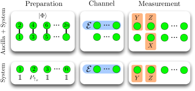
Figure 1: (Color online) Two equivalent ways to obtain the necessary measurements for the scalable process tomography scheme. Top row: System and ancilla are prepared in a maximally entangled state $|\Phi\rangle\propto\bigotimes_{i=1}^{N}[|0\rangle_{2i-1}|0\rangle_{2i}+|1\rangle_{2i-1}|1\rangle_{2i}]$ (with pairwise entanglement indicated by vertical lines), the channel $\mathcal{E}$ is applied on the system, and products of Pauli observables are measured on all blocks of $r$ consecutive sites (exemplified for $r=3$ and $\hat{\sigma}_{2}^{y}\otimes\hat{\sigma}_{3}^{x}\otimes\hat{\sigma}_{4}^{z}$), which serves as input to reconstruct the resulting state $\hat{\varrho}_{\mathcal{E}}$ and thus the channel $\mathcal{E}$. Bottom row: Equivalently, these expectation values may be obtained without the ancillary system. The initial states have eigenstates of Pauli matrices (here, $\hat{P}_{\uparrow_{x}}$, $\hat{P}_{\downarrow_{x}}$, so those of $\hat{\sigma}_{2}^{x}$) on those sites where a Pauli matrix would have been measured on the ancilla. After application of the channel, the system part of the ancilla + system measurement is carried out (here, that of $\hat{\sigma}_{1}^{y}\otimes\hat{\sigma}_{2}^{z}$).

The most straightforward approach to process tomography is based on the idea of probing the quantum channel with an informationally complete set of states. After sending each of these input states through the channel, the process underlying the dynamics is characterized by performing full state tomography on all of the output states. The so-obtained map fully characterizes the channel Nielsen and Chuang (2007); Chuang and Nielsen (1997); Poyatos et al. (1997). This strategy is referred to as standard quantum process tomography (SQPT) and works well as long as the underlying system is of low dimension. Considering multi-partite quantum systems, however, reveals the disadvantages of this technique: Not only the number of states to be sent through the channel and to be indentified grows exponentially with the number of subsystems $n$, but also the number of parameters that need to be determined for each of the output states. There is, however, a strategy to overcome the exponential scaling of the number of input and output states: ancilla-assisted process tomography (AAPT) D’Ariano and Lo Presti (2001); Dür and Cirac (2001); Altepeter et al. (2003); ft: (a). AAPT requires an ancillary system of the same size $n$ as the system itself, the preparation of a maximally entangled input state $|\Phi\rangle\propto\sum_{i}|i\rangle|i\rangle$ on the combined system, and full tomography of the resulting state after application of the channel, $\hat{\varrho}_{\mathcal{E}}=(\mathbbm{1}\otimes\mathcal{E})(|\Phi\rangle\!\langle\Phi|)$, see Fig. 1. This method is based on the correspondence between quantum states and quantum processes known as the Choi-Jamiołkowski isomorphism Choi (1975); Jamiołkowski (1972). The incorporation of an ancillary system considerably reduces the complexity of the preparation stage (as opposed to exponentially many input states in SQPT, only one state has to be prepared and only one output state has to be characterized) but comes at the cost of needing access to an independent ancilla system of the same size as the system that is to be analyzed. Still, for a complete characterization of the output state $\hat{\varrho}_{\mathcal{E}}$, a number of measurements exponentially large in $n$ is required Mohseni et al. (2008).

In this work, we combine recent results from efficient and scalable state tomography Cramer et al. (2010); Baumgratz et al. (2013b) with the idea of AAPT and discuss how to avoid the need for an ancilla system (see, e.g., Flammia et al. (2012); Bendersky et al. (2008)) as summarized in Fig. 1. This allows us to formulate a scalable process tomography scheme where the number of input and output states, together with the experimental measurement settings to characterize the latter, grows only linearly with the number of qubits.

We restrict our attention to unitary processes and demonstrate our scalable process tomography technique with numerical simulations of quantum circuits and of time evolution under local one-dimensional Hamiltonians. In Sec. III.1, we consider a circuit which prepares a Greenberg-Horne-Zeilinger (GHZ) state and the quantum Fourier transform. Note that the GHZ circuit is a limited-depth circuit (as defined below, cf. Jozsa (2006)), which implies that it has an efficient matrix product operator (MPO) representation in the sense that the bond dimension scales at most polynomially with the number of qubits. This is exactly the class of processes for which one would expect methods based on Refs. Cramer et al. (2010); Baumgratz et al. (2013b) to work. In turn, the quantum Fourier transform is a circuit of polynomial depth, but one that admits an approximate efficient simulation with a classical computer Yoran and Short (2007). For the $n=32$ qubits considered here, an MPO representation that approximates the circuit exists and our reconstruction scheme works well.

In Sec. III.2 we simulate process tomography for time evolutions of one-dimensional local Hamiltonians $\hat{H}$ and show how to extract the Hamiltonians from the reconstructed processes. The reconstruction of a Hamiltonian on $n$ qubits will require one process reconstruction at time $\sim 1/\|\hat{H}\|\sim 1/n$ (Sec. III.2.1) or two process reconstructions at times $t_{1}$, $t_{2}$ separated by no more than $\sim 1/\|\hat{H}\|$ (Sec. III.2.2). In the latter case, the only restriction on $t_{1}$ and $t_{2}$ is that the process admits reconstruction at those times. In both cases, the reconstruction of a Hamiltonian will require roughly $\sim\!n^{2}$ measurements of each of the $\sim\!n$ observables.

The quality of the reconstructed processes may be quantified using the same experimental resources that are also required to obtain the reconstruction: For unitary processes, $\hat{\varrho}_{\mathcal{E}}$ is guaranteed to be pure such that certifiability of the reconstruction of $\mathcal{E}$ is inherited by the certifiablity of $\hat{\varrho}_{\mathcal{E}}$ Cramer et al. (2010); see Ref. Kim (2014) for an analogous mixed-state certificate.

II Scalable Process Tomography

Let us first consider the AAPT scheme and restrict, without loss of generality, to qubits. Furthermore, we arrange the ancilla + system as depicted in Fig. 1 with odd sites representing the ancilla and even sites denoting the system itself. In this enumeration, the maximally entangled input state $|\Phi\rangle$ takes the form of a product of Bell states $|\phi^{+}\rangle_{1,2}\otimes\cdots|\phi^{+}\rangle_{2n-1,2n}$, $|\phi^{+}\rangle\propto|00\rangle+|11\rangle$, and hence only requires local two-qubit manipulations for its experimental generation. The system (i.e., the even sites) is sent through the channel and state tomography has to be performed on the resulting state $\hat{\varrho}_{\mathcal{E}}$. Without any prior knowledge about the underlying quantum channel, full state tomography is inevitable and one seemingly faces the notorious curse of dimensionality. A large class of quantum states, however, may be reconstructed from a number of measurements and with post-processing resources that both scale only polynomially in $n$ Cramer et al. (2010); Baumgratz et al. (2013a, b).

Post-processing with polynomial resources requires an efficient representation of the state, which, in one dimension, is provided by matrix product state (MPS) or operator (MPO) representations Fannes et al. (1992); Perez-Garcia et al. (2007); Schollwöck (2011), compare also tree tensor networks Shi et al. (2006) and the multiscale entanglement renormalization ansatz Vidal (2007). There are many examples of physical states that admit an efficient matrix product representation, e.g. ground states of gapped local Hamiltonians Hastings (2007); Plenio et al. (2005); Eisert et al. (2010), thermal states of local Hamiltonians Eisert et al. (2010); Hastings (2006) and entangled states like the GHZ state, the W state and cluster states.

If the output state $\hat{\varrho}_{\mathcal{E}}$ happens to be close to this class of states with an efficient matrix product representation, scalable reconstruction of the channel may be achieved. The input to the scalable state tomography schemes Cramer et al. (2010); Baumgratz et al. (2013a, b) are given by the measurement data of the following observables (or, alternatively, any other local operator basis):

$$\hat{P}_{k;\alpha_{1},\dots,\alpha_{r}}=\mathbbm{1}_{1,\dots,k}\otimes\hat{\sigma}^{\alpha_{1}}_{k+1}\otimes\cdots\otimes\hat{\sigma}^{\alpha_{r}}_{k+r}\otimes\mathbbm{1}_{k+r+1,\dots,2n},$$ (1)

for all $\alpha_{i}\in\{x,y,z\}$, $k=0,\dots,2n-r$, and a fixed $r$ independent of the size of the system. Here, $\hat{\sigma}_{i}^{x}$, $\hat{\sigma}_{i}^{y}$, $\hat{\sigma}_{i}^{z}$ are the Pauli matrices for qubit $i$. There are $(2n-r+1)\times 3^{r}$ such operators, i.e., the number of observables that are required for these reconstruction schemes scales linearly in $n$. Note that the restriction to local information is not mandatory, any output state that is uniquely characterized by a number of measurements that scales moderately with $n$ can be reconstructed by these techniques Baumgratz et al. (2013b) and, hence, belongs to the class of states for which our process tomography procedure is applicable.

Interestingly, the necessary information may also be obtained without the need of an ancilla (see, e.g., Flammia et al. (2012); Bendersky et al. (2008)), yet then increasing the demand at the preparation stage: By virtue of the identity

$$\text{tr}[(\hat{A}\otimes\hat{S})\hat{\varrho}_{\mathcal{E}}]=\frac{\text{tr}[\mathcal{E}(\hat{A}^{t})\hat{S}]}{2^{n}},\;\;\;\hat{A}^{t}=\sum_{i,j}\langle j|\hat{A}|i\rangle|i\rangle\langle j|,$$ (2)

which holds for any operator $\hat{S}$ ($\hat{A}$) acting on the system (ancilla), and the fact that each $\hat{P}_{k;\alpha_{1},\dots,\alpha_{r}}$ is of the form $\hat{P}_{A}\otimes\hat{P}_{S}$ ($A$: ancilla, $S$: system), one may obtain the necessary expectation values by preparing the eigenstates of the Pauli matrices in $\hat{P}_{A}$ on the system, sending them through the channel and measuring $\hat{P}_{S}$ on the resulting state (see Fig. 1 and Appendix A for details) – a scheme that requires no ancilla, the preparation of linearly many states and the measurement of linearly many observables.

While the preparation and measurement strategy we just outlined may be favourable from an experimental perspective, we will present our scheme in the framework of AAPT as certain intuitions are particularly transparent in this setting. In the remainder of this section, we discuss how unitary operators and the Hamiltonians governing time evolution can be constructed from $\hat{\varrho}_{\mathcal{E}}$. In principle, the scheme is applicable to non-unitary channels as well, as long as the corresponding state $\hat{\varrho}_{\mathcal{E}}$ permits reconstruction.

II.1 Reconstruction of Unitary Channels

We aim at reconstructing unitary channels, so channels of the form $\mathcal{E}(\hat{\varrho})=\hat{U}\hat{\varrho}\hat{U}^{\dagger}$. For those, it is guaranteed that the resulting state is pure, i.e., $\hat{\varrho}_{\mathcal{E}}=|\psi_{\mathcal{E}}\rangle\langle\psi_{\mathcal{E}}|$. The unitary may then be obtained from the identity $\langle j|\hat{U}|i\rangle=2^{n/2}\langle i|\langle j|\psi_{\mathcal{E}}\rangle$. The output of the state reconstruction algorithms of Refs. Cramer et al. (2010); Baumgratz et al. (2013b) provide us with a pure estimate $|\psi^{\text{rec}}_{\mathcal{E}}\rangle$ of $\hat{\varrho}_{\mathcal{E}}$ given in the form of a matrix product state (MPS) Fannes et al. (1992); Perez-Garcia et al. (2007),

$$|\psi^{\text{rec}}_{\mathcal{E}}\rangle=\sum_{i_{1},\ldots,i_{2n}}A^{(1)}_{i_{1}}\cdots A^{(2n)}_{i_{2n}}|i_{1},\ldots,i_{2n}\rangle,$$ (3)

where $A^{(k)}_{i_{k}}\in\mathbb{C}^{D_{k-1}\times D_{k}}$ with $D_{0}=1=D_{2n}$ and summation is over all $i_{k}=1,2$; $k=1,\ldots,2n$. The $D_{k}$ are called bond dimensions. Given this form, the matrix product operator (MPO) representation of the estimate $\hat{U}_{\text{rec}}$ to $\hat{U}$, $\langle j|\hat{U}_{\text{rec}}|i\rangle=2^{n/2}\langle i|\langle j|\psi^{\text{rec}}_{\mathcal{E}}\rangle$, may straightforwardly be obtained by grouping the $n$ pairs of ancilla and system sites:

$$\hat{U}_{\text{rec}}=2^{\frac{n}{2}}\sum_{i_{1},\ldots,i_{2n}}\Bigl{[}A_{i_{1}}^{(1)}A_{i_{2}}^{(2)}\Bigr{]}\cdots\Bigl{[}A_{i_{2n-1}}^{(2n-1)}A_{i_{2n}}^{(2n)}\Bigr{]}\,\,|i_{2}\rangle\!\langle i_{1}|\otimes\cdots\otimes|i_{2n}\rangle\!\langle i_{2n-1}|.$$ (4)

As the input state $|\Phi\rangle$ can efficiently be represented as an MPS (given the sites are labeled as depicted in Fig. 1), the process $\hat{U}$ having an efficient MPO representation will imply that the exact state $|\psi_{\mathcal{E}}\rangle$ has an efficient MPS representation, and successful reconstruction may be possible. We now show that circuits with an at most logarithmic depth have an efficient MPO representation. Our condition is equivalent to the condition given in Ref. Jozsa (2006), but we give a tighter bound on the bond dimension. Let a circuit $\hat{U}$ be composed of $N$ two-qubit gates,

$$\hat{U}=\prod_{j=1}^{N}\hat{U}_{j},\quad\hat{U}_{j}\text{ acts on }l_{j}\text{ and }r_{j}>l_{j}.$$

We define the depth of the circuit at the bipartition $i|i+1$ by

$$d_{i}=|\{j\colon l_{j}\leq i\text{ and }r_{j}\geq i+1\}|$$

and denote the maximal depth by $d_{\text{max}}=\max_{i}d_{i}$. This definition is motivated by the fact that an MPO representation of $\hat{U}$ with bond dimension at most $4^{d_{\text{max}}}$ is easily obtained from the MPO representations of the $\hat{U}_{j}$: The $\hat{U}_{j}$ have bond dimension $D_{i}\leq 4$ for $l_{j}\leq i\leq r_{j}-1$ and $D_{i}=1$ everywhere else, and the bond dimension of the product $\hat{U}$ is given, in the worst case, by $D_{i}(\hat{U})=\prod_{j=1}^{N}D_{i}(\hat{U}_{j})$ Schollwöck (2011). If the depth $d_{\text{max}}$ grows at most logarithmically with $n$, we obtain an MPO representation of the circuit that is efficient in the sense that it has a number of parameters at most polynomial in $n$.

II.2 Hamiltonian Reconstruction

Assume that the quantum process is in fact the time evolution under a local one-dimensional Hamiltonian, i.e., $\hat{U}=\mathrm{e}^{-\mathrm{i}\hat{H}t}$, with $\hat{H}=\sum_{i}\hat{h}_{i}$, where $\hat{h}_{i}$ only acts on a fixed number of neighbouring sites (we will consider nearest-neighbour Hamiltonians throughout) and where $\|\hat{h}_{i}\|\leq J$ for a constant $J$. With the tools to reconstruct unitary processes at hand, it remains to address the question of how to find a valid estimate of the Hamiltonian $\hat{H}$ governing the time evolution. To obtain $\hat{H}$ from this unitary, we will use the identity

$$x =\sin(x)\frac{\arccos(\cos(x))}{\sqrt{1-(\cos(x))^{2}}}, x \in(-\pi,\pi),$$ (5)

together with the power series

$$\frac{\arccos(z)}{\sqrt{1-z^{2}}} =\sum_{k=0}^{\infty}c_{k}(z-1)^{k}, c_{k}=\frac{(-1)^{k}}{2^{k}}\prod_{j=1}^{k}\frac{j}{j+\frac{1}{2}}$$ (6)

which converges for $|z-1|<2$ [][.Printcompantionto:NISTDigitalLibraryofMathematicalFunctions.\url{http://dlmf.nist.gov/}; Release1.0.9of2014-08-29.DerivedfromEq.~4.24.2; availableat\url{http://dlmf.nist.gov/4.24\#E2}.]Olver2010nocompanion. The basic idea is that from $\hat{U}=\mathrm{e}^{-\mathrm{i}\hat{H}t}$, we know that $2\mathrm{i}\sin(\hat{H}t)=\hat{U}^{\dagger}-\hat{U}$, $2\cos(\hat{H}t)=\hat{U}^{\dagger}+\hat{U}$, and Eq. (5) holds up to times limited by $\|\hat{H}t\|<\pi$. While this appears to limit the accessible time interval for Hamiltonian reconstruction, Sec. III.2.2 will explain how to extend this result to longer times.

For practical purposes, we only want to evaluate a finite number of terms of the series in Eq. (6) and enforce Hermiticity. To this end, we approximate

$$\hat{H}_{\text{rec}}t=\frac{1}{2}\sin(\hat{H}_{\text{rec}}t)\sum_{k=0}^{N-1}c_{k}(\cos(\hat{H}_{\text{rec}}t)-\mathbbm{1})^{k}+\text{h.c.}$$ (7)

for a given $N$ and $\sin(\hat{H}_{\text{rec}}t)$ and $\cos(\hat{H}_{\text{rec}}t)$ as above. This approach has two advantages over using a power series expansion of the logarithm: It is valid for larger values of $\|Ht\|$ and the series converges much faster. Note that even if the reconstruction of $|\psi_{\mathcal{E}}\rangle$ is perfect, $\hat{U}_{\text{rec}}$ may differ from $\hat{U}$ by a global phase $\phi$, such that $\hat{U}_{\text{rec}}^{\dagger}\mathrm{e}^{\mathrm{i}\phi}\hat{U}=\mathbbm{1}$ and Eq. (5) imposes $\|Ht-\phi\mathbbm{1}\|<\pi$. To remedy this problem, we use $\hat{U}_{\text{rec}}\operatorname{{tr}}(\hat{U}_{\text{rec}})^{*}/|\operatorname{{tr}}(\hat{U}_{\text{rec}})|$ as our actual estimate.

The initial state $|\Phi\rangle$ is an MPS of low bond dimension and, as under local Hamiltonians quantum correlations build up in a light-cone-like picture, $|\psi_{\mathcal{E}}\rangle$ will still have a small bond dimension for small times Eisert and Osborne (2006); Bravyi et al. (2006). More precisely, at a fixed time, there is an approximate MPO representation of $U$ with a bond dimension that grows at most polynomially with the number of qubits Osborne (2006). In our numerical simulations on $n\leq 32$ qubits, we observe that a MPS representation is feasible at times on the order of $1/J$.

III Numerical Simulations

We carry out numerical simulations as follows: For several exemplary channels $\mathcal{E}$, we numerically obtain $|\psi_{\mathcal{E}}\rangle$ as detailed below and simulate measurements of the local observables $\hat{P}_{k;\alpha_{1},\dots,\alpha_{r}}$ by drawing $M$ times per observable according to $|\psi_{\mathcal{E}}\rangle$. In this way, we take statistical errors into account, with statistical errors for measurements without ancilla being very similar ft: (b). The resulting empirical mean values (i.e., the simulated estimates of the weights $\langle\hat{\Pi}_{k;\alpha_{1},\ldots,\alpha_{r}}^{s_{1},\ldots,s_{r}}\rangle_{\hat{\varrho}_{\mathcal{E}}}$ of all eigenprojectors $\hat{\Pi}_{k;\alpha_{1},\ldots,\alpha_{r}}^{s_{1},\ldots,s_{r}}$, $s_{i}=\pm 1$, of $\hat{P}_{k;\alpha_{1},\ldots,\alpha_{r}}$) are then used to obtain a reconstruction $|\psi_{\mathcal{E}}^{\text{rec}}\rangle$ of $|\psi_{\mathcal{E}}\rangle$. This is done by exploiting the singular-value-thresholding-like algorithm described in Cramer et al. (2010) to obtain an initial state for the scalable maximum-likelihood algorithm of Ref. Baumgratz et al. (2013b). The result is an MPS representation of $|\psi_{\mathcal{E}}^{\text{rec}}\rangle$ which can be converted into an MPO representation of $\hat{U}_{\text{rec}}$ as described above in Eq. (4).

With the estimate $|\psi_{\mathcal{E}}^{\text{rec}}\rangle$ and thus the corresponding operator $\hat{U}_{\text{rec}}$ at hand, we then quantify the quality of the reconstruction scheme by

$$F=F(\hat{U},\hat{U}_{\text{rec}})=|\langle\psi_{\mathcal{E}}|\psi^{\text{rec}}_{\mathcal{E}}\rangle|^{2},$$ (8)

and note that this is in one-to-one correspondence to other distance measures for unitary channels used in the literature Raginsky (2001); Gilchrist et al. (2005); Pedersen et al. (2007); ft: (c).

In the case of Hamiltonian reconstruction, we assess our reconstructed estimates as follows: First, note that two Hamiltonians $\hat{H}$ and $\hat{H}+\lambda\mathbbm{1}$, $\lambda\in\mathbb{R}$, are physically indistinguishable. Therefore, we measure relative distances between Hamiltonians according to ft: (d)

$$D(\hat{H},\hat{H}^{\prime}) =\frac{\min_{\lambda\in\mathbb{R}}\|\hat{H}-\hat{H}^{\prime}-\lambda\mathbbm{1}\|}{\min_{\lambda\in\mathbb{R}}\|\hat{H}-\lambda\mathbbm{1}\|},$$ (9)

which is independent of energy offsets in both $\hat{H}^{\prime}$ and $\hat{H}$. We choose the operator norm $\|\cdot\|$ motivated by its property

$$|\langle\hat{A}(t)\rangle_{\hat{\varrho}}-\langle\hat{A}^{\prime}(t)\rangle_{\hat{\varrho}}|\leq 2|t|\|\hat{H}-\hat{H}^{\prime}\|\|\hat{A}\|,$$

where $\hat{A}(t)$ and $\hat{A}^{\prime}(t)$ are the Heisenberg picture time evolutions of $\hat{A}$ according to $\hat{H}$ and $\hat{H}^{\prime}$, respectively. In other words, the operator norm distance defines a timescale on which two Hamiltonians may be considered equivalent.

For all results below, we repeat the whole procedure of sampling from the simulated state, reconstructing it, and assessing the quality of the reconstruction several times. All results shown are mean values of $F(\hat{U},\hat{U}_{\text{rec}})$ and $D(\hat{H},\hat{H}_{\text{rec}})$ over a small number of runs, with deviations that are, for the number of measurements per observable considered, smaller than the size of the markers. Next, we present numerical results for the reconstruction of quantum circuits and Hamiltonians and study the performance as a function of the number of qubits $n$, the number $M$ of measurements per observable, and the block size $r$ of the subsystems on which measurements are performed. We simulate circuits and Hamiltonians on up to $32$ qubits. Hence, reconstructing the unitary uses pure state reconstruction on up to $64$ qubits.

III.1 Quantum Circuits

We demonstrate the feasibility of our scalable tomography scheme by considering the $\widehat{\text{GHZ}}$ circuit, which prepares an $n$-qubit GHZ state from $|0\ldots 0\rangle$ and the quantum Fourier transform Nielsen and Chuang (2007),

$$\begin{split}\widehat{\text{GHZ}}&=\widehat{\text{CN}}_{n-1,n}\widehat{\text{CN}}_{n-2,n-1}\cdots\widehat{\text{CN}}_{1,2}\hat{H}_{1},\\ \widehat{\text{QFT}}&=\prod_{k=1}^{n}\Biggl{[}\Biggl{(}\prod_{j=1}^{n-k}\widehat{\text{CR}}_{k,k+j}(\pi/2^{j})\Biggr{)}\hat{H}_{k}\Biggr{]},\end{split}$$ (10)

where we use the convention $\prod_{j=1}^{k}\hat{U}_{i}=\hat{U}_{k}\cdots\hat{U}_{1}$ for products of non-commuting operators. Here, $\hat{H}_{k}$ denotes the Hadamard gate acting on qubit $k$, and $\widehat{\text{CN}}_{i,i+1}$ ($\widehat{\text{CR}}_{i,j}(\phi)$) denotes the two-qubit conditional-NOT (conditional rotation) gate Nielsen and Chuang (2007). The $\widehat{\operatorname{GHZ}}$ circuit has depth $d_{\text{max}}=1$ and thus admits an exact efficient MPO representation. The depth of the exact quantum Fourier transform circuit is $d_{\text{max}}=\lfloor\frac{n^{2}}{4}\rfloor$ and grows quadratically with the number of qubits (see Appendix B). However, one can obtain an approximation $\widehat{\operatorname{QFT}}_{c}$ of the quantum Fourier transform by dropping all conditional rotations with $j>c$ from the definition in Eq. (10) Coppersmith (1994). This approximation can be simulated classically with polynomial resources Yoran and Short (2007). Using numerical MPO compression techniques Schollwöck (2011), we obtain an approximate MPO representation with bond dimension 16 and error bounded by $[2(1-\sqrt{F})]^{1/2}<2\times 10^{-5}$ for the $n\leq 32$ qubits we consider.

The reconstruction results are summarized in Fig. 2. The reconstruction of the $\widehat{\operatorname{GHZ}}$ performs very well. To discuss the performance of the quantum Fourier transform reconstruction, we note that the distance $\epsilon_{c}$ between the exact quantum Fourier transform and its approximation $\widehat{\operatorname{QFT}}_{c}$ is upper bounded by $\epsilon_{c}\leq n\pi/2^{c}$ (see Yoran and Short (2007) and Appendix B). We reconstruct $\widehat{\operatorname{QFT}}$ with high fidelity $F\approx 0.99$ from measurements on $r=5$ consecutive qubits on the combined system + ancilla (Fig. 1). Naively, one would expect to be able to reconstruct $\widehat{\operatorname{QFT}}_{c}$ only for $c\leq 2$, because $r=5$ corresponds to information about three neighbouring system qubits only. However, the upper bound on the approximation error is trivial for $c=2$ and $8\leq n\leq 32$, and numerical tests show that the actual approximation error $\epsilon_{c}$ is indeed several times larger than the reconstruction error $[2(1-\sqrt{F})]^{1/2}$ we achieve. This shows that there are non-local gates which can be reconstructed without using the corresponding non-local information.

Figure 2: (Color online) Reconstruction of the quantum circuits in Eq. (10). Figures show the fidelity in Eq. (8) of the exact unitary and its tomographic reconstruction as a function of the system size $n$ for $M=\infty$ (left) and as a function of the number $M$ of measurements per local observable for different $n$ (right). Reconstruction uses measurements on all blocks of $r$ consecutive qubits only. Lines are guides to the eye. The numerical data suggest a linear scaling of $(1-\sqrt{F})^{1/2}$ with system size $n$ and $1/\sqrt{M}$.

III.2 Hamiltonian reconstruction

III.2.1 Short times

We simulate the time evolution $\hat{U}$ of time-independent local one-dimensional Hamiltonians $\hat{H}$ with well-established numerical DMRG/MPO algorithms ft: (e). After obtaining the estimate $\hat{U}_{\text{rec}}$ of the time evolution, we determine an estimate $\hat{H}_{\text{rec}}$ of the Hamiltonian that governs the time evolution by the series given in Eq. (7) with $N=3$. With this, and the assumption that $\min_{\lambda\in\mathbb{R}}\|\hat{H}-\lambda\mathbbm{1}\|=\|\hat{H}\|$ ft: (f), one has

$$D(\hat{H},\hat{H}_{\text{rec}}) \leq\tfrac{\|\hat{H}-\hat{H}_{\text{rec}}\|}{\|\hat{H}\|}\leq\tfrac{1}{140}\|\hat{H}t\|^{6}+O(\|\hat{H}t\|^{8}).$$ (11)

Fig. 3 shows results for an isotropic Heisenberg Hamiltonian on $n\leq 32$ qubits. We have also studied the critical Ising model and a Hamiltonian with random nearest-neighbour interaction, which show very similar behaviour and the corresponding results may be found in Appendix C. We use $t_{n}=1/\|\hat{H}\|$ as a time unit and recall that the local terms of the Hamiltonian are bounded by a constant, $\|\hat{h}_{i}\|\leq J$. This gives us $t_{n}\geq 1/nJ$ and $t_{n}\sim 1/n$ if we additionally assume that the local terms all have similar norm.

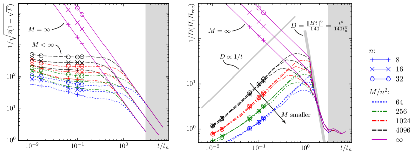
Figure 3: (Color online) Left: Fidelity between exact state $|\psi_{\mathcal{E}}\rangle$ and tomographic estimate $|\psi_{\mathcal{E}}^{\text{rec}}\rangle$ of a unitary time evolution $\hat{U}=\mathrm{e}^{-\mathrm{i}\hat{H}t}$, with $\hat{H}$ the isotropic Heisenberg Hamiltonian on $n$ qubits. The tomographic estimate is based on complete measurements on blocks of $r=3$ consecutive qubits with $M$ measurements per observable. Right: Inverse relative distance $D$ between $\hat{H}$ and $\hat{H}_{\text{rec}}$ reconstructed from $|\psi_{\mathcal{E}}^{\text{rec}}\rangle$. The unit of time is $t_{n}=1/\|\hat{H}\|\sim 1/n$, i.e., inversely proportional to the number of qubits, and the grey area indicates where reconstruction is expected to fail due to Eq. (5). The grey lines without any markers show the expected behaviour for small times and times near $\pi$ (see Eq. (11) and the main text). The data indicates that for $M<\infty$, $M/n^{2}$ fixed and $t/t_{n}$ fixed and sufficiently small, $D(\hat{H},\hat{H}_{\text{rec}})$ is largely independent of $n$.

The distance $D(\hat{H},\hat{H}_{\text{rec}})$ between the reconstructed and the exact Hamiltonian shown in Fig. 3 displays the following features: First, the reconstruction is expected to fail for $\|\hat{H}t\|\geq\pi$ (see Eq. (5)) and, indeed, $D(\hat{H},\hat{H}_{\text{rec}})$ is large in this area (indicated by the grey background). Secondly, Eq. (11) suggests that close to $\|\hat{H}t\|=\pi$, $D(\hat{H},\hat{H}_{\text{rec}})$ should scale as $\|\hat{H}t\|^{6}/140=t^{6}/(140t_{n}^{6})$ (thick grey line in Fig. 3). Thirdly, we observe that for infinitely many measurements per observable, $M=\infty$, and fixed $t/t_{n}=\|\hat{H}\|t\sim nt$, the distance $D(\hat{H},\hat{H}_{\text{rec}})$ decreases with system size, a behaviour inherited from the quality of the reconstruction $|\psi^{\text{rec}}_{\mathcal{E}}\rangle$ (see left of Fig. 3): The fidelity $F(\hat{U},\hat{U}_{\text{rec}})$ is limited by the amount of block entanglement in $|\psi_{\mathcal{E}}\rangle$. At a fixed time $t$, an area law Eisert et al. (2010) holds for this entanglement such that it is bounded even for arbitrarily large systems Eisert and Osborne (2006); Bravyi et al. (2006). For sufficiently large systems, we hence expect $F(\hat{U},\hat{U}_{\text{rec}})$ at fixed $t$ to be independent of the system size $n$. If we keep $t/t_{n}\sim t\cdot n$ fixed, we therefore expect $F$ to increase with $n$. Finally, let us discuss the dependence of the distance between the exact and the reconstructed Hamiltonian in Fig. 3 on the number $M$ of measurements per observable. First of all, with a finite number of measurements no reconstruction will be possible at small times, because the signal of the Hamiltonian in $\hat{U}\approx\mathbbm{1}-\mathrm{i}\hat{H}t$ will be smaller than the noise. Furthermore, the data suggests that, for times before $t/t_{n}\approx\pi$,

$$D(\hat{H},\hat{H}_{\text{rec}})\propto \frac{1}{t/t_{n}}\frac{n}{\sqrt{M}}.$$ (12)

This is the behaviour one would expect if one assumes that the relative error $D(\hat{H},\hat{H}_{\text{rec}})$ is proportional to the ratio $R/S$ of a noise amplitude $R$ and the strength of the signal $S=\|\hat{H}t\|=t/t_{n}$, in which $R=n/\sqrt{M}$ is motivated by the fact that we have measured $\propto n$ observables, each of which has been estimated to within a standard deviation given, for sufficiently large $M$, by $1/\sqrt{M}$.

The explanation of the scaling properties together with the fact that all properties described are the same in the other Hamiltonians investigated (see Appendix C) suggest that that the scaling laws apply for many local Hamiltonians on a linear chain, for a large range of system sizes and any sufficiently large (as indicated by the examples) number of measurements.

To summarize, measuring at larger times gives a larger signal and a smaller error, but we are limited by the condition $t/t_{n}<\pi$ imposed by Eq. (5). Solving Eq. (12) for the number of measurements per observable, we obtain $M\propto n^{2}(t/t_{n})^{2}/D^{2}$: A constant relative error $D$ at a fixed $t/t_{n}<\pi$ requires $M\propto n^{2}$ measurements per observable, resulting in a total number of measurements proportional to $n^{3}$ .

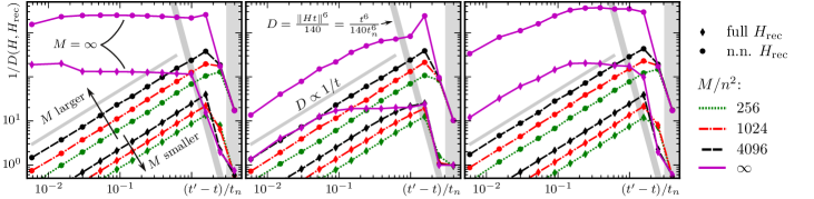
Figure 4: (Color online) Quality of the reconstruction $\hat{H}_{\text{rec}}$ for $\hat{H}$ the critical Ising (left), isotropic Heisenberg (middle) and a random nearest-neighbour Hamiltonian (right). $\hat{H}_{\text{rec}}$ was obtained from $U(t^{\prime}-t)$ with $t/t_{n}=3.51$ fixed and $U(t^{\prime}-t)=U^{\dagger}U^{\prime}$ was obtained from tomographic estimates of $U=\mathrm{e}^{-\mathrm{i}\hat{H}t}$ and $U^{\prime}=\mathrm{e}^{-\mathrm{i}\hat{H}t^{\prime}}$. The inverse relative error $1/D(\hat{H},\hat{H}_{\text{rec}})$ is shown for $H_{\text{rec}}$ (diamonds) and for the projection of $H_{\text{rec}}$ onto a nearest-neighbour Hamiltonian (circles). $\hat{H}$ acts on $n=32$ qubits and tomographic estimates are based on complete measurements on blocks of $r=5$ consecutive qubits with $M$ measurements per observable. The unit of time is $t_{n}=1/\|\hat{H}\|\sim 1/n$. Most properties are similar to Fig. 3 right where $\hat{H}_{\text{rec}}$ was reconstructed from an estimate of $U(t)$, with the time difference $t^{\prime}-t$ taking the role of the time $t$. Lines are guides to the eye.

III.2.2 Long times

In its present formulation, the reconstruction scheme is limited to $t/t_{n}<\pi$, a restriction that may be overcome by measuring at two different times $t$, $t^{\prime}$: The times up to which the fidelity $F(\hat{U},\hat{U}_{\text{rec}})$ is sufficiently high is only limited by $r$ – increasing $r$ will increase the time up to which full information about $\hat{U}$ may be obtained by measuring on $r$ consecutive qubits. In fact, as can be seen on the left of Fig. 3, for $n=32$ and the relatively small $r=3$, the fidelity $F(\hat{U},\hat{U}_{\text{rec}})$ is still quite high at $t/t_{n}=\pi$ while the reconstruction of $\hat{H}$ fails for these times. Measuring at $t$, $t^{\prime}$ and obtaining $\hat{U}=\mathrm{e}^{-\mathrm{i}\hat{H}t}$, $\hat{U}^{\prime}=\mathrm{e}^{-\mathrm{i}\hat{H}t^{\prime}}$ by reconstruction, we are only limited by $|t^{\prime}-t|<\pi t_{n}$ when reconstructing $\hat{H}$ from $\hat{U}^{\dagger}\hat{U}^{\prime}=\mathrm{e}^{\mathrm{i}\hat{H}(t-t^{\prime})}$. Fig. 4 shows results of this reconstruction scheme with $t/t_{n}=3.51$ and $t^{\prime}>t$.

Reconstructing the Hamiltonian from $\hat{U}(t^{\prime}-t)=\hat{U}^{\dagger}\hat{U}^{\prime}$, the time difference $t^{\prime}-t$ clearly assumes the role of the time $t$ when reconstructing the Hamiltonian from $\hat{U}$ at time $t$ alone. Therefore, all scaling properties carry over as long as $\hat{U}_{\text{rec}}$ and $\hat{U}^{\prime}_{\text{rec}}$ can be obtained with sufficiently high fidelity. We simulated measurements on blocks of $r=5$ consecutive sites to satisfy this requirement.

For exact measurements, $M=\infty$, the relative error $D(\hat{H},\hat{H}_{\text{rec}})$ does not approach zero for $t^{\prime}-t\to 0$. The reason is that the error in $\hat{U}_{\text{rec}}(t^{\prime}-t)$ remains non-zero as $t^{\prime}-t\to 0$ because $\hat{U}_{\text{rec}}(t)$ has a fixed non-zero error at fixed $t$. This non-zero error may also become larger than the signal amplitude $\|\hat{H}t\|$, explaining the increasing error as $t^{\prime}-t\to 0$ for some of the Hamiltonians.

Note that, from $\hat{U}(t^{\prime}-t)$, we can also reconstruct Hamiltonians that are time-dependent for times before $t$ and nearly constant between $t$ and $t^{\prime}$. In this way, stroboscopic reconstructions of a time-dependent Hamiltonian may be obtained after large propagation times. Furthermore, $t/t_{n}<\pi$ becomes more restrictive as $n$ increases, thus the usefulness of taking measurements at two times increases for larger systems.

III.2.3 Enforcing a local reconstruction

Of course, making use of additional information can only improve the scheme. As an example, suppose that we know that the Hamiltonian is nearest-neighbour only. One may then project the reconstructed $\hat{H}_{\text{rec}}$ onto a nearest-neighbour Hamiltonian. As can be seen in Fig. 4, this reduces the error dramatically.

IV Conclusion and Outlook

We studied in detail the application of recent scalable state tomography models to quantum process tomography. At the hand of unitary channels—quantum circuits such as logarithmic-depth circuits, the quantum Fourier transform and unitary time-evolution governed by one-dimensional local Hamiltonians—favourable scaling with the number of qubits was numerically demonstrated. The scheme, as presented, relies on an ancilla system, the preparation of a maximally entangled state on the combined system, and local measurements after application of the channel. We also discussed an alternative scalable scheme without the need for an ancilla, which displays the same scaling properties as the ancilla-assisted scheme. The quality of the reconstructed unitary channel may be quantified using the certificate introduced in Ref. Cramer et al. (2010).

We have also shown how one-dimensional local Hamiltonians may be reconstructed from their corresponding unitary after an evolution time inversely proportional in the size $n$ of the system and requiring $\propto n^{2}$ measurements of each of $\propto n$ observables. We have discussed and numerically demonstrated how the restriction of these small evolution times may be relaxed by taking measurements at two different times. This enables the reconstruction and verification of a quantum device at arbitrarily large times for as long as the conditions for efficient state tomography are met, even if, intermittently, the device has passed through highly entangled states. Furthermore, the knowledge of the Hamiltonian being local may be incorporated and has, for the Hamiltonians that we studied, improved fidelities considerably.

Using the mixed-state tomography methods introduced in Refs. Baumgratz et al. (2013a, b), we expect non-unitary channels to be similarly amenable to the scheme studied here. Assessing the quality of such a reconstruction, however, will rely on the ability to quantify the quality of mixed-state reconstructions – a goal that is, in particular for many qubits and sufficient generality, still to be met.

Appendix A Technical Details on Ancilla-Assisted Tomography and the Reduction of Experimental Effort

Let

$$|\Phi\rangle=\frac{1}{2^{n/2}}\sum_{i=1}^{2^{n}}|i\rangle|i\rangle$$ (13)

be the maximally entangled state on the combined system. Then

$$\hat{\varrho}_{\mathcal{E}}=(\mathbbm{1}_{A}\otimes\mathcal{E})(|\Phi\rangle\!\langle\Phi|)=\frac{1}{2^{n}}\sum_{i,j}|i\rangle\langle j|\otimes\mathcal{E}(|i\rangle\langle j|),$$ (14)

i.e., $\langle i|\langle j|\hat{\varrho}_{\mathcal{E}}|i^{\prime}\rangle|j^{\prime}\rangle=\langle j|\mathcal{E}(|i\rangle\langle i^{\prime}|)|j^{\prime}\rangle/2^{n}$ and $\hat{\varrho}_{\mathcal{E}}$ thus completely characterizes the channel $\mathcal{E}$. We now review a known scheme (see, e.g., Flammia et al. (2012); Bendersky et al. (2008)) for obtaining measurement data on $\hat{\varrho}_{\mathcal{E}}$ from measurements that use preperation and measurement on the system without the ancilla. In addition, we show that the linearly many product observables required for scalable state tomography schemes Cramer et al. (2010); Baumgratz et al. (2013a, b) may be obtained from linearly many simple product preperations and product measurements. In the simplest case, the schemes require the observables

$$\hat{P}_{k;\alpha_{1},\dots,\alpha_{r}}=\mathbbm{1}_{1,\dots,k}\otimes\hat{\sigma}^{\alpha_{1}}_{k+1}\otimes\cdots\otimes\hat{\sigma}^{\alpha_{r}}_{k+r}\otimes\mathbbm{1}_{k+r+1,\dots,2n}\;\;\text{with}\;\;\alpha_{i}\in\{x,y,z\}\;\;\text{and}\;\;k=0,\dots,2n-r,$$ (15)

where $\hat{\sigma}_{i}^{x}$, $\hat{\sigma}_{i}^{y}$, $\hat{\sigma}_{i}^{z}$ are the Pauli matrices on site $i$. Measuring these observables, we obtain the expectation values of the eigenprojectors

$$\hat{\Pi}_{k;\alpha_{1},\ldots,\alpha_{r}}^{s_{1},\ldots,s_{r}} =\mathbbm{1}_{1,\ldots,k}\otimes\hat{\Pi}_{k+1;\alpha_{1}}^{s_{1}}\otimes\ldots\otimes\hat{\Pi}_{k+r;\alpha_{r}}^{s_{r}}\otimes\mathbbm{1}_{k+r+1,\ldots,2n},\;\;\text{where}\;\;\hat{\Pi}^{s_{i}}_{k+i;\alpha_{i}}=|\alpha_{i},s_{i}\rangle\langle\alpha_{i},s_{i}|,\quad s_{i}\in\{-1,1\},$$ (16)

with Pauli matrix eigenstates defined by $\hat{\sigma}^{\alpha_{i}}|\alpha_{i},s_{i}\rangle=s_{i}|\alpha_{i},s_{i}\rangle$.

For given $\hat{\Pi}_{k;\alpha_{1},\ldots,\alpha_{r}}^{s_{1},\ldots,s_{r}}$, write $\hat{\Pi}_{k;\alpha_{1},\ldots,\alpha_{r}}^{s_{1},\ldots,s_{r}}=\hat{P}_{A}\otimes\hat{P}_{S}$ with the direct product referring to ancilla ($A$) vs. system ($S$). One finds

$$\begin{split}\langle\hat{P}_{A}\otimes\hat{P}_{S}\rangle_{\hat{\varrho}_{\mathcal{E}}}&=\text{tr}[\hat{\varrho}_{\mathcal{E}}(\hat{P}_{A}\otimes\hat{P}_{S})]=\frac{1}{2^{n}}\sum_{i,j,k,l}\langle i|\langle j|\bigl{[}\bigl{(}|k\rangle\langle l|\hat{P}_{A}\bigr{)}\otimes\bigl{(}\mathcal{E}(|k\rangle\langle l|)\hat{P}_{S}\bigr{)}\bigr{]}|i\rangle|j\rangle\\ &=\frac{1}{2^{n}}\sum_{i,j,k,l}\langle i|\bigl{(}|k\rangle\langle l|\hat{P}_{A}\bigr{)}|i\rangle\langle j|\bigl{(}\mathcal{E}(|k\rangle\langle l|)\hat{P}_{S}\bigr{)}|j\rangle=\frac{1}{2^{n}}\sum_{i,j,l}\langle l|\hat{P}_{A}|i\rangle\langle j|\mathcal{E}(|i\rangle\langle l|)\hat{P}_{S}|j\rangle\\ &=\frac{1}{2^{n}}\sum_{i,l}\langle l|\hat{P}_{A}|i\rangle\text{tr}[\mathcal{E}(|i\rangle\langle l|)\hat{P}_{S}]=\frac{1}{2^{n}}\text{tr}[\mathcal{E}(\hat{P}_{A}^{t})\hat{P}_{S}],\end{split}$$ (17)

where $\hat{P}_{A}^{t}=\sum_{i,l}\langle l|\hat{P}_{A}|i\rangle|i\rangle\langle l|$ is the transpose of $\hat{P}_{A}$ in the basis in which $|\Phi\rangle$ is entangled. Note that $\hat{P}_{A}$ is, up to a prefactor, a mixed product state. The expectation value $\langle\hat{P}_{A}\otimes\hat{P}_{S}\rangle_{\hat{\varrho}_{\mathcal{E}}}$ may thus be obtained by preparing the state $\hat{P}_{A}$, sending it through the channel and measuring an appropriate product of Pauli matrices on the output state.

Appendix B Quantum Fourier Transform Gate Properties

The quantum Fourier transform circuit is given by (cf. Eq. (10) in the main text)

$$\widehat{\text{QFT}} =\prod_{k=1}^{n}\Biggl{[}\Biggl{(}\prod_{j=1}^{n-k}\widehat{\text{CR}}_{k,k+j}(\pi/2^{j})\Biggr{)}\hat{H}_{k}\Biggr{]}$$

As one two-qubit gate acts on every pair of qubits, the depth (defined in Sec. II.1 of the main text) at the split $i|i+1$ is given by $d_{i}=i(n-i)$, the maximal depth is $d_{\text{max}}=\max_{i}d_{i}=\lfloor\frac{n^{2}}{2}\rfloor$ and there is an MPO representation with bond dimension $D\leq 4^{d_{\text{max}}}=4^{\lfloor n^{2}/2\rfloor}$, which is not efficient. However, we can obtain a smaller bond dimension as follows: The conditional rotation gates are given by $\widehat{\operatorname{CR}}_{k,k+j}(\phi)=|0\rangle_{k}\langle 0|\otimes\mathbbm{1}_{k+j}+|1\rangle_{k}\langle 1|\otimes R_{k+j}(\phi)$ with $R(\phi)=|0\rangle\!\langle 0|+\mathrm{e}^{\mathrm{i}\phi}|1\rangle\!\langle 1|$. Observe that

$$\prod_{j=1}^{n-k}\widehat{\text{CR}}_{k,k+j}(\pi/2^{j}) =|0\rangle_{k}\!\langle 0|\otimes\mathbbm{1}_{k+1,\ldots,n}+|1\rangle_{k}\!\langle 1|\otimes R_{k+1}(\pi/2)\otimes\ldots\otimes R_{n}(\pi/2^{n-k}).$$

The two summands on the right-hand side are tensor products and thus have an MPO representation with bond dimension 1. Therefore, the left-hand side has an MPO representation with bond dimension 2 Schollwöck (2011). Concatenating the $n$ terms of this form, we obtain an MPO representation of $\widehat{\operatorname{QFT}}$ with bond dimension $2^{n}$, which still is not efficient.

As mentioned in the main text, an approximation of the quantum Fourier transform can be simulated classically with polynomial resources Yoran and Short (2007). Using numerical MPO compression techniques Schollwöck (2011), we obtain a feasible approximate MPO representation of the quantum Fourier transform circuit on $n\leq 32$ qubits: At bond dimension 16, the error is bounded by $[2(1-\sqrt{F})]^{1/2}<2\times 10^{-5}$.

Because the quantum Fourier transform circuit contains many small conditional rotations, one can try to approximate the circuit by a circuit $\widehat{\operatorname{QFT}}_{c}$ obtained by dropping all conditional rotations from Eq. (10) in the main text with $j>c$ Coppersmith (1994). The operator norm error satisfies (see also Yoran and Short (2007))

$$\|\widehat{\operatorname{QFT}}-\widehat{\operatorname{QFT}}_{c}\| \leq\sum_{k=1}^{n}\sum_{j=c+1}^{n-k}\|\mathbbm{1}-\widehat{\operatorname{CR}}(\pi/2^{j})\|\leq\pi\sum_{k=1}^{n}\sum_{j=c+1}^{n-k}\frac{1}{2^{j}}\leq n\pi\sum_{j=c+1}^{\infty}\frac{1}{2^{j}}=\frac{n\pi}{2^{c}}$$

The operator norm error in turn upper bounds our error measure $[2(1-\sqrt{F})]^{1/2}$: For two unitaries $U$, $U^{\prime}$ and with the Frobenius norm $\|M\|_{F}=\operatorname{{tr}}(M^{\dagger}M)$,

$$2(1-\sqrt{F})=\min_{\alpha\in\mathbb{R}}\||\psi_{U}\rangle-\mathrm{e}^{\mathrm{i}\alpha}|\psi_{U^{\prime}}\rangle\|_{2}^{2}\leq\||\psi_{U}\rangle-|\psi_{U^{\prime}}\rangle\|_{2}^{2}=\frac{\|U-U^{\prime}\|_{F}^{2}}{2^{n}}\leq\|U-U^{\prime}\|^{2}.$$

Appendix C Hamiltonian Reconstruction for Ising and Random Hamiltonians

Fig. 3 in the main text shows the performance of our reconstruction scheme for local Hamiltonians using the example of the isotropic Heisenberg Hamiltonian. Fig. 5 shows data for the critical Ising model and for a Hamiltonian with random nearest-neighbour interaction, with matrix elements chosen uniformly from $[-1,1]$. Reconstruction works equally well for the critical Ising model and the randomly chosen nearest-neighbour interaction.

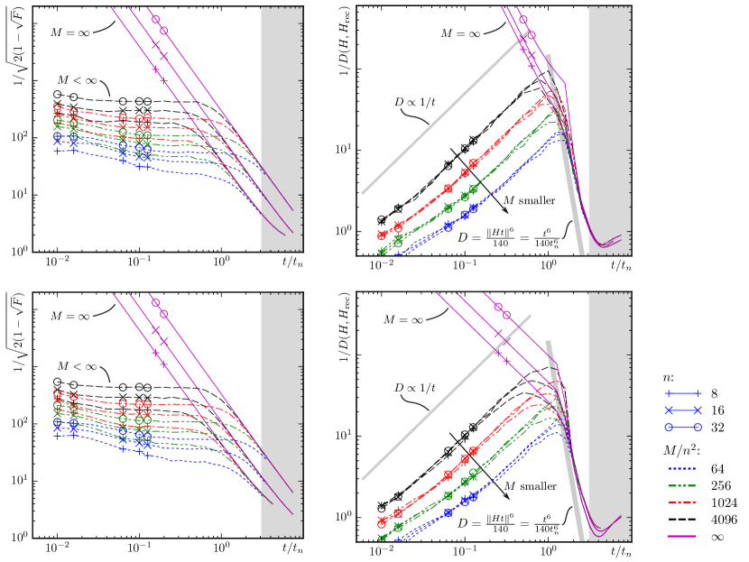
Figure 5: (Color online) Left: Fidelity between exact state $|\psi_{\mathcal{E}}\rangle$ and tomographic estimate $|\psi_{\mathcal{E}}^{\text{rec}}\rangle$ for a unitary time evolution $\hat{U}=\mathrm{e}^{-\mathrm{i}\hat{H}t}$ with $\hat{H}$ the Hamiltonian of the critical Ising model (top row) and a Hamiltonian with random nearest-neighbour interaction (bottom row). The Hamiltonians act on $n$ qubits and the tomographic estimate is based on complete measurements on blocks of $r=3$ consecutive qubits with $M$ measurements per observable. Right: Inverse relative distance between $\hat{H}$ and $\hat{H}_{\text{rec}}$ reconstructed from $|\psi_{\mathcal{E}}^{\text{rec}}\rangle$. The unit of time is $t_{n}=1/\|\hat{H}\|\sim 1/n$. Results are very similar to the isotropic Heisenberg data shown in Fig. 3 in the main text.