Fluctuation-induced first-order phase transitions in type-1.5 superconductors in zero external field

Abstract

In a single-component Ginzburg-Landau model which possesses thermodynamically stable vortex excitations, the zero-field superconducting phase transition is second order even when fluctuations are included. Beyond the mean-field approximation the transition is described in terms of proliferation of vortex loops. Here we determine the order of the superconducting transition in an effective 3D vortex-loop model for the recently proposed multiband type-1.5 superconductors. The vortex interaction is nonmonotonic, i.e., exponentially screened and attractive at large separations, and short-range repulsive. We show that the details of the vortex interaction, despite its short-range nature, can lead to very different properties of the superconducting transition than found in type-1 and type-2 systems. Namely, the type-1.5 regime with nonmonotonic intervortex interaction can have a first-order vortex-driven phase transition not found in the single-band case.

I Introduction

The order of the zero-field superconducting transition has been studied in many works in the usual single-component type-1 and type-2 superconductors. Halperin, Lubensky, and Ma established that in extreme type-1 superconductors the gauge field fluctuations render the superconducting phase transition first order Halperin et al. (1974); Coleman and Weinberg (1973). In the opposite limit of extreme type-2 systems, Dasgupta and Halperin Dasgupta and Halperin (1981) demonstrated that the superconducting transition is continuous and in the universality class of the inverted-3DXY model. The different nature of the superconducting phase transition in this limit is revealed by a duality mapping Dasgupta and Halperin (1981); Peskin (1978); Thomas and Stone (1978), which demonstrates that the phase transition is driven by proliferation of vortex-loop fluctuations.

While the extreme type-1 and type-2 limiting cases are well investigated, the value of Ginzburg-Landau parameter $\kappa=\lambda/\xi$ at which the phase transition changes from second to first order is much harder to establish. The attempted analytical approaches Kleinert (1982) are based on approximations that are unfortunately not controllable, in contrast to the well controllable duality mapping in the London limit Dasgupta and Halperin (1981); Peskin (1978); Thomas and Stone (1978). The most reliable information to date comes from numerical simulations. The largest Monte Carlo simulations performed so far Mo et al. (2002); Hove et al. (2002) claim that the tricritical $\kappa_{\text{tri}}=\left(0.76\pm 0.04\right)/\sqrt{2}$ is slightly smaller than the critical $\kappa_{c}=1/\sqrt{2}$, which separates the type-1 regime with thermodynamically unstable vortices and the type-2 regime with thermodynamically stable vortices. In these works it is claimed that even in the weakly type-1 regime where the vortex interaction is purely attractive and vortices are not thermodynamically stable, the phase transition can be continuous.

Recently it has been proposed that in multicomponent superconductors there is a new regime that falls outside the type-1/type-2 classification. Such materials are described by theories with multiple superconducting components, e.g., by Ginzburg-Landau theory of the form

$$F=\sum_{a=1,2}\frac{1}{2}|(i\nabla-e{\bf A})\psi_{a}|^{2}+V(|\psi_{a}|,\theta_{1}-\theta_{2})+\frac{(\nabla\times{\bf A})^{2}}{2}$$ (1)

where $\psi_{a}=|\psi_{a}|e^{i\theta_{a}}$ are superconducting components, $V$ is a collection of potential terms, and ${\bf A}$ is the vector potential. Such systems have multiple coherence lengths $\xi_{a}$. For detailed discussion of the definitions of coherence lengths in the presence of inter-component coupling, see Ref. Carlström et al., 2011. In type-1.5 regimes some of the coherence lengths are larger and some are smaller than the magnetic field penetration length $\lambda$ Babaev and Speight (2005); Babaev et al. (2010); Carlström et al. (2011). The different coherence lengths can originate from the existence of different superconducting gaps in different bands Silaev and Babaev (2011), or superconducting states breaking multiple symmetries Carlström et al. (2011); Agterberg et al. (2014).

In what follows we focus on the two-band case. It has been shown that thermodynamically stable double-core vortices exist in the regime where $\xi_{1}<\sqrt{2}\lambda<\xi_{2}$. In 2D such vortices asymptotically have an interaction of the form Babaev and Speight (2005); Babaev et al. (2010); Carlström et al. (2011)

$$V(r)\sim m^{2}K_{0}\left(r/\lambda\right)-q_{1}^{2}K_{0}\left(r/\xi_{1}\right)-q_{2}^{2}K_{0}\left(r/\xi_{2}\right)$$ (2)

where $m,q_{1},q_{2}$ are system dependent coefficients and $K_{0}$ is a modified Bessel function. The first term in Eq. (2)n with range $\lambda$ originating from the magnetic and current-current interaction is repulsive for two vortices with like vorticity and attractive otherwise. The second and third terms are attractive with range $\xi_{L}=\max\left\{\xi_{1},\xi_{2}\right\}$, and originate from core-core interaction for vortices with two cocentered overlapping cores in the two superconducting components. Consequently in type-1.5 regime with $\xi_{L}>\lambda$ the interaction is short-range repulsive due to the first term, while at the longer range it is exponentially screened and attractive due to the core-core attraction. We will refer to the core-core attraction as intermediate-range attractive to emphasize that all interactions here are exponentially screened. In contrast to the type-1 regime, type-1.5 systems have thermodynamically stable vortex excitations, while in contrast to the type-2 regime the intermediate-range intervortex forces are attractive. Therefore the nature of the superconducting phase transition in the type-1.5 systems cannot be deduced from known cases of single-component superconductors. Currently the problems of type-1.5 superconductivity is a subject of intense experimental research on materials where vortex clusters were observed Moshchalkov et al. (2009); Ray et al. (2014); Gutierrez et al. (2012); Nishio et al. (2010); Hicks et al. (2010).

Similar to the single-component case, in two-band systems it is difficult to advance analytically in a controllable way away from extremely type-2 regimes, in particular using duality arguments. Nonetheless one can identify a limit in the type-1.5 regime where certain simplifying assumptions can be made. That is, consider a two-band superconductor with relatively strong interband coupling made of a strongly type-2 component and a type-1 component with a much lower ground state density. This condition implies that vortex excitations are expected to drive the phase transition. Yet in contrast to type-2 superconductors, the vortices will feature a small attractive tail in the interaction. In a regime with relatively strong interband coupling, vortices can be approximated as objects with no fluctuating internal structure, and, under certain conditions, multibody forces between type-1.5 vortices can be neglected Carlström et al. (2011). Then the composite vortices can be seen as charged point particles interacting via a sum of screened Coulomb potential terms.

In this paper we study the 3D vortex-loop driven finite-temperature superconducting phase transition in zero field for a model of a type-1.5 superconductor. The main task is to investigate the order of the superconducting transition. We propose an effective model for composite vortices with a nonmonotonic length scale dependence of the vortex interaction. We study this model by classical finite-temperature Monte Carlo (MC) simulation and finite-size scaling methods in order to classify the order of the transition. From the U(1) symmetry of the superconducting order parameter an inverted 3DXY transition is the expected result for a system with thermodynamically stable vortices, but instead we obtain first-order transitions in the cases involving a nonmonotonic vortex interaction that we tested. This result differs qualitatively from the single-band systems where the zero field transition driven by thermodynamically stable vortices is considered to be always continuous.

II Generalized effective vortex loop model

For the type-1.5 regime in the limit outlined above, fluctuations near the phase transition can be expected to be described by a generalized 3D vortex loop model that we will now formulate. In a 3D system vortex lines form closed loops, and on a lattice the vortex degrees of freedom become directed integer link current variables $q_{i}^{\sigma}$, where $\sigma=\hat{x},\hat{y},\hat{z}$ are the unit lattice vectors connecting the site $i$ with its neighbor $i+\sigma$ on a simple cubic lattice with vertices $i=1,\dots,L^{d}$. The numerical lattice constant is set to unity. The functions $K_{0}(r/\lambda)$ in Eq. (2) generalize to 3D Yukawa interactions, represented on a lattice with periodic boundary conditions by lattice Green’s functions

$$Y_{ij}=Y\left(\frac{\left|\mathbf{r}_{i}-\mathbf{r}_{j}\right|}{\lambda_{Y}}\right)=\frac{c_{Y}}{L^{d}}\sum_{\mathbf{k}}\frac{\cos\left(\mathbf{k}\cdot\left(\mathbf{r}_{i}-\mathbf{r}_{j}\right)\right)}{6-\sum_{\sigma}{2\cos\left(k_{\sigma}\right)}+\lambda_{Y}^{-2}}$$ (3)

where $c_{Y}$ is a real coupling constant. The 3D counterpart of Eq. (2) is then given by the vortex line Hamiltonian

$$H=\sum_{i,j,\sigma}\frac{1}{2}q_{i}^{\sigma}V_{ij}q_{j}^{\sigma}+\sum_{i,j,\sigma}\frac{1}{2}\left|q_{i}^{\sigma}\right|U_{ij}\left|q_{j}^{\sigma}\right|$$ (4)

where both $U_{ij}$ and $V_{ij}$ shall have the form of Eq. (3). The first term corresponds to $m^{2}K_{0}\left(r/\lambda\right)$ in Eq. (2) with $\lambda_{V}=\lambda$ in Eq. (3). Thus $V_{ij}$ mediates the screened Coulomb interaction of the composite vortex lines as obtained for a two-component 3D superconductor with range set by the London penetration depth $\lambda$. The second term corresponds to the slowest decaying density interaction $-q_{L}^{2}K_{0}\left(r/\xi_{L}\right)$ in Eq. (2), which is always attractive ($c_{U}<0$) and of exactly the same form as $V_{ij}$ with range $\lambda_{U}=\xi_{L}$. The faster decaying component has been ignored meaning that its range and amplitude are assumed to be sufficiently small. This model is highly simplified and neglects amplitude fluctuations, additional core-energy contributions, and core-core interactions between perpendicular line segments. While such effects can in principle be included in the model to reach accurate description of a given material, we here focus on properties of the effective model and leave more detailed investigations for future work.

For a weak attractive part $\left|c_{U}\right|\ll c_{V}$ and $\xi_{L}\leq\lambda$, Eq. (4) is similar to a type-2 superconductor, and from the U(1) symmetry of the model it is expected that the transition from the ordered low-temperature phase to the disordered high-temperature phase is a second-order phase transition belonging to the inverted 3DXY universality class. However for a general choice of parameters in Eq. (4) such an a priori assertion is not possible. The order of the transition must in general be determined by simulations or by other means.

Next we discuss the choice of parameter values. The possible parameter choices are restricted by a stability criterion in order to represent a valid description for multicomponent superconductors. That is, the coefficients $c_{U}<0<c_{V}$ and the ranges $\lambda,\xi_{L}$ in Eq. (4) must be chosen such that the lowest energy state is the vortex free state with all the $q_{i}^{\sigma}=0$. At the parameters we will consider the minimum of the vortex interaction comes from the attraction energy between nearest neighbor link variables with opposite sign. A candidate low energy state is thus given by a Néel-type stacked loop configuration on a cubic lattice such as $q^{z}\left(\mathbf{r}\right)=\left(-1\right)^{x+y+z},q^{y}\left(\mathbf{r}\right)=-q^{z}\left(\mathbf{r}\right),q^{x}\left(\mathbf{r}\right)=0$. The energy of the stacked state can be calculated from the Hamiltonian in Fourier space, $H=\frac{1}{2L^{d}}\sum\limits_{\sigma,{\bf k}}\left[\tilde{V}({\bf k})|\tilde{q}^{\sigma}({\bf k})|^{2}+\tilde{U}({\bf k})|\tilde{Q}^{\sigma}({\bf k})|^{2}\right]$, where $Q^{\sigma}(\mathbf{r})=|q^{\sigma}(\mathbf{r})|$, which gives $E=L^{d}[\tilde{V}(\pi,\pi,\pi)+\tilde{U}(0,0,0)]=L^{d}[c_{V}/(12+\lambda^{-2})+c_{U}\xi_{L}^{2}]$. The boundary of stable parameters is identified by setting this energy to zero to make the stacked state degenerate with the vortex-free vacuum state. The parameters used in the model must thus satisfy

$$\frac{c_{V}}{12+\lambda^{-2}}+c_{U}\xi_{L}^{2}>0$$ (5)

To investigate the different types of behavior of the model in Eq. (4) we focus on several different parameter regimes:

(1) Screened repulsive parameters (SR): $\xi_{L}=\lambda=0.5,c_{V}=41,c_{U}=-2.5$. The attractive coefficient $c_{U}$ is small compared to $c_{V}$ yielding a net repulsive interaction between vortex segments with equal vorticity, thus representing a two-band type-2 superconductor. The transition in this model is therefore expected to belong to the inverted-3DXY universality class, which will be verified below.

(2) Nonmonotonic parameters (NM): $\xi_{L}=1,\lambda=0.5,c_{V}=41,c_{U}=-2.5$. The range $\xi_{L}$ of the attractive part has been increased compared to the SR case yielding an effectively nonmonotonic interaction with a net repulsion at short length scales and a net attraction at intermediate length scales between equal vorticities. For these values of $\xi_{L},\lambda,c_{U}$, the choice $c_{V}=41$ is within the stability requirement $c_{V}>40$ given by Eq. (5). This regime gives a simplified effective model for vortex loops in type-1.5 superconductors.

(3-4) Screened repulsive parameters with enhanced attraction (SR10, SR1024999): $\lambda=\xi_{L}=0.5,c_{V}=41$ and $c_{U}=-10,-10.24999$, respectively, which are close to the minimum allowed value $-10.25$ set by Eq. (5). For the SR1024999 parameters the vortex free state and the staggered configuration are almost degenerate in energy. In ordinary superconductors the energy of such vortex configurations contain contributions from nonpairwise forces, which are not present in our model. In this parameter regime the model is not representative for currently known ordinary superconductors and has mainly theoretical interest.

III Calculated quantities and scaling arguments

Destruction of superconductivity in systems with thermodynamically stable vortices is associated with proliferation of vortex loop fluctuations. For finite $\lambda$ we can assume an ensemble where number fluctuations of the vortex lines are included at finite energy cost. The proliferation of vortex loops at the phase transition is signaled by fluctuations in the winding numbers

$$W_{\sigma}=\frac{1}{L}\sum_{i}q_{i}^{\sigma}$$ (6)

The singular behavior at a second-order phase transition is described by the finite size scaling ansatz

$$\langle W_{\sigma}^{2}\rangle=\tilde{W}^{2}(L^{1/\nu}t)$$ (7)

where $\tilde{W}^{2}$ is a scaling function, $L$ is the system size, $t=T/T_{c}-1$, and $\nu$ is the correlation length critical exponent. This means that curves of MC simulation data of $\langle W_{\sigma}^{2}\rangle$ vs temperature $T$ for different system sizes $L$ will intersect at $T=T_{c}$. The derivative scales as $\partial\langle W_{\sigma}^{2}\rangle/\partial T\sim L^{1/\nu}$ at the transition. For the 3DXY universality class the critical exponent for the correlation length is $\nu\approx 0.671$ and for the heat capacity $\alpha=2-d\nu\approx-0.015$ Campostrini et al. (2001).

In the vicinity of a first-order transition the two different phases coexist, the correlation length is finite, and scaling given by Eq. (7) is not fulfilled. Precisely at $T_{\text{c}}$ the system is equally probable to be in either of the phases. In simulations the internal energy histogram $P(e)$, where $e=H/L^{d}$ is the energy density, shows a double-peak structure centered around the two characteristic internal energy values $H_{1},H_{2}$. The free-energy barrier given by $\Delta F_{L}=(1/\beta)\log\left[{P_{\text{max}}}/{P_{\text{min}}}\right]$ increases with system size and behaves asymptotically as $L^{d-1}$ Lee and Kosterlitz (1990). For a second-order transition the double-peak structure disappears in the thermodynamic limit.

The presence of a double-peak structure in the energy histogram is not enough to distinguish between a first- and a second-order transition. For a first-order transition it is also required that the latent heat $\Delta H=H_{1}-H_{2}$ does not vanish in the thermodynamic limit. The latent heat contributes to the heat capacity

$$c_{L}\left(T\right)=\frac{\langle\left(H-\langle H\rangle\right)^{2}\rangle}{T^{2}L^{d}}$$ (8)

A double-peak structure in $P(e)$ leads to a heat capacity maximum at the transition with a leading size dependence given by $c_{L}^{*}\sim L^{d}(\Delta e)^{2}\sim L^{d}$, corresponding to a delta-function singularity at $T_{c}$ for $L\to\infty$. This is equivalent to an energy peak separation given by $\Delta e\sim(c_{L}^{*}/L^{d})^{1/2}>0$. On the contrary, if the transition is continuous the scaling form $c_{L}(T)\approx a(t,L)t^{-\alpha}+b(t)\approx L^{\alpha/\nu}\tilde{a}\left(L^{1/\nu}t\right)+b(t)$ holds. This implies that the maximum $c_{L}^{*}$ grows slower upon increasing the system size than in the case of a first-order transition as long as $d\nu>1$, and a histogram with a single energy peak. In the data analysis below we sometimes find it useful to plot the rescaled heat capacity $c_{L}/L^{d}$ which for increasing system size should approach a constant maximum for a first order transition and a decreasing maximum for a 3DXY transition. To reduce the influence of the analytic term it can be beneficial to consider the third moment Smiseth et al. (2003)

$$M_{3}=\langle H-\langle H\rangle\rangle^{3}\sim\frac{\partial}{\partial T}\left(T^{2}L^{d}c_{L}\right)$$ (9)

This quantity exhibits two extrema around $T_{\text{c}}$ whose difference $\Delta M_{3}$ scales as $\sim L^{\frac{1+\alpha}{\nu}}$ for continuous and $\sim L^{2d}$ for discontinuous transitions. The size dependence of $c_{L}^{*}$ and $\Delta M_{3}$ at a first-order transition corresponds to effective exponents $\alpha=1,\nu=1/d$.

In addition a method by Challa, Landau, and BinderChalla et al. (1986) which does not rely on a precision determination of the energy histogram can be used to determine the order of a transition. The reduced fourth order energy cumulant for system size $L$ is

$$V_{L}=1-\frac{\langle H^{4}\rangle}{3\langle H^{2}\rangle^{2}}$$ (10)

For both discontinuous and continuous transitions this quantity approaches the trivial limit $V^{*}_{\infty}=2/3$ for $T\neq T_{\text{c}}$. For finite-size systems a minimum $V_{L}<V^{*}_{\infty}$ is obtained at the transition. For second-order transitions this minimum converges towards $V^{*}_{\infty}$ for $L\to\infty$, while for first-order transitions the minimum approaches a nontrivial value $V_{\infty}<V^{*}_{\infty}$ with a correction term $\sim L^{-d}$.

IV Monte Carlo methods

Our MC simulations use a hybrid scheme combining worm and exchange methods that performs well both at first- and second-order phase transitions. The classical worm algorithm Prokof’ev and Svistunov (2001) constructs closed vortex loop fluctuations in terms of closed random walk trajectories, and gives efficient simulation performance at a second-order phase transition by minimizing critical slowing down of the dynamics. In addition the replica exchange algorithm Hukushima and Nemoto (1996) is used in order to reduce the autocorrelation time and the risk of getting stuck in metastable states, which reduces hysteresis at first-order transitions. In our simulations we use 8-80 parallel threads. Prior to each production run the system was equilibrated for $2^{15}$ sweeps for the SR parameters, for at least $2^{17}$ sweeps for the NM and SR1024999 parameter sets, and for $2^{16}$ sweeps for the SR10 set. A MC sweep is taken to be $3L^{d}$ link variable updating attempts. Equally many sweeps were done to compute averages. The MC trajectories were then further analyzed using the multihistogram reweighting technique Ferrenberg and Swendsen (1989). Error bars are obtained via reweighting of different bootstrap realizations of the same MC trajectory. As a consistency check we also performed parallelized Wang-Landau simulations Wang and Landau (2001); Vogel et al. (2013) for the NM case in a finite energy window determined by the energy expectation value of the MC simulations. In the WL simulations the MC moves used are two types of closed loops, formed as attempts to insert closed elementary plaquette loops or as straight lines that close on themselves by the periodic boundary conditions. Consistent results between the different methods were obtained.

V Results

We start within the strong type-2 regime with model parameters given by the SR set with a repulsive short-range interaction. Figure 1 (A) shows MC results for the winding number fluctuations. At a second-order phase transition data curves of the winding number fluctuations vs temperature for different system sizes $L$ must intersect at the transition temperature according to Eq. (7). Corrections to scaling produce deviations from the intersection point visible in the figure for the smallest system sizes, but the biggest sizes intersect within error bars at a single temperature that estimates $T_{c}$. The inset in Fig. 1 (A) shows a finite-size scaling collapse of MC data for the four largest system sizes $L=20,22,24,26$ onto a single curve representing the scaling function $\tilde{W}^{2}$ in Eq. (7). In the scaling collapse the value $\nu=0.671$ of the 3DXY model was used. This is consistent with a second-order phase transition in the inverted-3DXY universality class as expected for short range repulsive interactions.

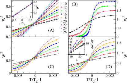
Figure 1: (Color online) MC data for vortex loop winding number fluctuations. (A) SR data curves intersect at the critical temperature $T_{\text{c}}\approx 1.386$, with scaling corrections visible for the smallest system sizes. Inset: finite size scaling data collapse for $L=20,22,24,26$ with $\nu=0.671$. (B) NM model. The onset is steeper than for the SR model, which indicates a first-order transition. (C) SR10 model with $c_{U}=-10$. (D) SR1024999 model with $c_{U}=-10.24999$. Inset: maximum of the winding number fluctuation derivative $dW^{2}/dT$ for all data sets. All curves have been normalized by the value obtained for $L=8$. The dashed blue line corresponds to a power law $\sim L^{3}$ and the dotted line to $\sim L^{4}$.

To investigate the effect of a nonmonotonic vortex interaction, MC data for $W^{2}$ for the NM parameter set is shown in Fig. 1 (B). The data deviates clearly from 3DXY scaling since the slope $dW^{2}/dT$ at the transition is much steeper than the 3DXY relation $L^{1/0.671}$ found in (A). This demonstrates that the transition of the NM model is not of the 3DXY type, and it will become clear below that it is instead first order. Panels (C) and (D) show data for the repulsive SR10 and SR1024999 models, respectively. The inset in (D) plots the maximum of $dW^{2}/dT$. Data curves for the SR and SR10 models both show deviations from a pure power law form for the system sizes studied here. The SR data indicates approach to the 3DXY result $L^{1/0.671}$ for large $L$ but corrections to power-law scaling are visible also for the largest lattice sizes. The SR10 model data show a possible slow crossover towards 3DXY scaling, but the sizes are too small to decide. The SR1024999 model is consistent with the size dependence $dW^{2}/dT\sim L^{3}$, showing no tendency for a crossover to 3DXY scaling for the range system sizes examined here. For the NM model the data scales approximately as $\sim L^{(d+1)}=L^{4}$. This suggests that the assumption of a universal scaling distribution for the winding number fluctuations $\sim L^{0}$ at the transition does not hold and indicates that the NM model has a first-order transition.

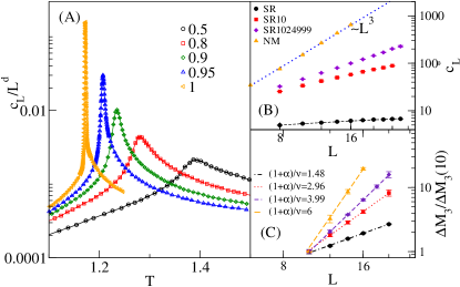
Figure 2: (Color online) MC data for the rescaled heat capacity and $M_{3}$. (A) $c_{L}/L^{d}$ vs $T$ for $L=14$ for a sequence of models ranging from the SR model with $\xi_{L}=0.5$ to the NM model with $\xi_{L}=1$. (B) Scaling of the maxima of $c_{L}$ vs $L$ for the different parameter sets. The dashed black line is a fit to the form $aL^{\omega}+b$ with $\omega=-0.02$ and the dotted blue line is a pure power law with $\omega=d=3$. (C) Scaling of $\Delta M_{3}$ vs $L$ normalized by the value at $L=10$. The NM and SR curves scale with the exponents expected for a first-order and inverted-3DXY transition, respectively.

Results for the heat capacity and energy histograms are shown in Figs. 2 and 3. Figure 2 (A) shows the evolution of MC data for the heat capacity $c_{L}$ for a sequence of parameter values in $\xi_{L}=0.5-1$ interpolating from the SR to NM case for system size $L=14$. The SR data curve is smooth, while increasing $\xi_{L}$ increases the peak height and decreases the width. The NM curve peaks sharply at the transition in agreement with a delta-function peak in the heat capacity at a first-order transition. The insets Figs. 2 (B) and 2(C) show the maximum value $c_{L}^{*}$ and the difference $\Delta M_{3}$ vs $L$. For the SR model good agreement is found with $c_{L}^{*}\sim L^{2/\nu-3}$ and $\Delta M_{3}\sim L^{(3-d\nu)/\nu}$ with $\nu=0.671$ as expected for the inverted-3DXY scenario. In the NM case the heat capacity maxima scale as $c_{L}^{*}\sim L^{d}$ and $\Delta M_{3}\sim L^{2d}$ indicating a strong first-order transition. Neither of the SR10 and SR1024999 sets show any tendency towards the same behavior, which suggests either a slow approach to second order or to weak first-order transitions. In both SR10 and SR1024999 cases much bigger system sizes are required for definite conclusions.

Figure 3 shows energy histograms at the transition temperature for the NM model and reveals a double-peak structure. The results from the Worm and Wang-Landau methods are similar, but the latter gives smoother data curves in the region between the peaks. Figure 3 (B) indicates that the latent heat saturates at a finite value for large system sizes, and (C) shows that the free-energy barrier grows with increasing system size. This indicates that the NM model has a strong first-order transition which is our main result.

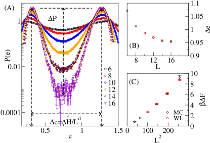
Figure 3: (Color online) (A) MC results for the energy histogram at the transition for the NM model. The probability density $P(e)$ exhibits a characteristic double-peak structure with a monotonically growing barrier $\Delta P$ upon increasing the system size. The dashed curves shown for $L=14,16$ are results of Wang-Landau calculations. (B) The normalized latent heat $\Delta e$ obtained from the maxima in (A) approaches a nonzero value for $L\rightarrow\infty$. (C) The free-energy barrier determined in (A) grows with increasing system size which indicates a strong first-order transition.

The transition in the models SR10 and SR1024999 is more difficult to categorize. Energy histograms for the SR10 model did not produce any double peaks for the system sizes we explored. The heat capacity peak in the inset in Fig. 2 increases significantly slower than a $\sim L^{3}$ law expected for a first-order transition, and may possibly approach 3DXY scaling for large systems for the SR10 model. Both these results favor a second-order transition.

Figure 4 shows energy histogram data for the SR1024999 model. Figure 4 (A) shows a double-peak structure in the histogram. Figure 4 (B) shows a free energy barrier growing slowly with increasing system size which is expected at a first-order transition. However, the heat capacity maximum plotted in Fig. 2 (B) grows slower than a $L^{d}$ power law corresponding to a first-order transition, indicating that the width of the energy histogram $\Delta e\to 0$ for $L\to\infty$. While this suggests a continuous transition, two further observations can be made. The scaling deviation from first-order behavior could in principle be attributed to finite size corrections as follows. The width of the energy histogram in Fig. 4 (A) is related to the heat capacity data in Fig. 2 by $\Delta e_{L}\sim(L^{-d}c_{L})^{1/2}$. A finite size scaling ansatz $\Delta e_{L}=\Delta e_{\infty}+A/L+B/L^{2}$ with fit parameters $\Delta e_{\infty},A,B$, gives a good fit to the data and extrapolates to a finite peak width $\Delta e_{\infty}\approx 0.18$ in the large system limit, which is consistent with a first-order transition showing substantial finite size corrections. Alternatively, a power law of the form $\Delta e_{L}\sim 1/L^{p}$ also fits the data and gives $p\approx 0.7$, which extrapolates to a single delta peak histogram for $L\to\infty$. This corresponds to a heat capacity maximum that varies with system size as $c_{L}^{*}\sim L^{1.6}$. However, as also seen in Figs. 2 (B) and (C), this is far from the finite-size scaling behavior expected at a 3DXY transition given by $c_{L}^{*}\approx aL^{-0.02}+b$.

Figure 4 (C) shows results for the minimum of the energy cumulant $V_{L}$. All data curves can be fitted to the form $V_{L}=V_{\infty}+aL^{-b}$. Data for the SR model quickly converges towards the expected value $V_{\infty}=2/3$ for a second-order transition. A fit of the data for the SR10 model gives $V_{\infty}=0.66\pm 0.01$ which is consistent with a second-order transition. The corresponding fit for the SR1024999 model gives a slightly lower asymptotic limit $V_{\infty}=0.64\pm 0.01$, but with a correction exponent $b\approx 1.9$ rather than $b=d=3$ expected for a strong first-order transition. The NM model gives a negative minimum value of $V_{L}$ for all $L$ consistent with a strong first-order transition (data not shown).

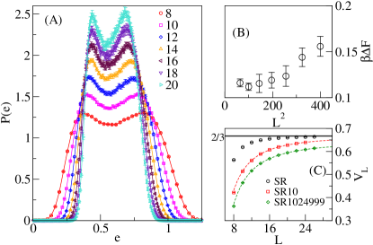
Figure 4: (Color online) (A) Energy histogram of the SR1024999 model at the phase transition. The tendency towards double-peak formation is much weaker than for the NM case plotted in Fig. 3. (B) The free-energy barrier $\Delta F$ increases slowly with system size. (C) Minimum value of the energy cumulant $V_{L}$ vs system size $L$. The black line is the asymptotic limit 2/3 expected for second order transitions. Dashed curves are fits to the form $V_{L}=V_{\infty}+a/L^{b}$.

To further assess the importance of nonmonotonicity in the vortex interaction we implemented the following modification of the NM model. The attractive potential $U_{ij}$ in Eq. (4) of the NM model was set to zero beyond a cutoff radius $r_{c}$ without altering the interaction for $r<r_{c}$. Taking the cutoff radius to $r_{c}=3$ gives a totally repulsive interaction in all directions. The effect of truncating the interaction at different distances is demonstrated in Fig. 5, which indicates that for $r_{c}=3$ the first-order behavior vanishes and the transition becomes second order, presumably turning into a 3DXY transition as for the SR case. The energy histograms in this case have no double-peak structure. If the cutoff radius is chosen to $r_{c}=5$ the interaction becomes nonmonotonic in all directions. Then the first-order signature reappears as shown by the black curve and the double-peaked energy histogram in the inset in Fig. 5. This indicates that the first-order mechanism found in the NM model is affected by the nonmonotonicity of the vortex interaction.

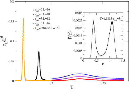
Figure 5: (Color online) Rescaled heat capacity for different cutoff lengths of the NM model interaction. The NM model without truncation (orange curve) has a first-order transition with a sharp peak in the heat capacity. The truncated model with $r_{c}=3$ (blue, purple, red curves) has a monotonic interaction, and gives a rescaled heat capacity peak that decreases with system size indicating a second-order transition. For the nonmonotonic model with $r_{c}=5$ (black curve) first-order signatures reappear, i.e., a sharp heat capacity peak, and a double-peaked energy histogram at the transition (inset).

Taken together the results in Figs. 1, 2 and 5 suggest $d\nu>1$ for all models with a screened monotonic interaction. This implies a collapse of the histogram in Fig. 4 to a single peak in the thermodynamic limit, and thus second-order transitions for all SR models. However, given the results presented in Fig. 4 and the fact that the exponents for the SR10 and SR1024999 data in Figs. 1 and 2 clearly deviate from the 3DXY values, weak first-order transitions in the thermodynamic limit cannot be completely ruled out. The model then would have weak first-order transitions also for parameters where the interaction between vortices is fully repulsive. Again, in this near degenerate regime the model does not correspond to ordinary type-2 superconductors.

VI Discussion

We present simulation results suggesting that in type-1.5 superconductors there is a new mechanism that drives the superconducting transition to become first order. This however does not imply that the superconducting phase transition in type-1.5 material is generically first order. We described the fluctuations by a generalized effective link-current model. To answer the question in the general case requires much more computationally demanding large-scale simulations of full two-band Ginzburg-Landau models. It is conceivable that fluctuation-induced enhancement of the repulsion for some of the parameters of the model eliminates the bare attractive interaction between vortices, which may make the phase transition continuous for certain parameter ranges in the type-1.5 regime. Among various scenarios for realization of type-1.5 superconductivity, a special reservation should be made for simple $U(1)$ multiband materials. In that particular case, at the mean-field level, the intervortex interaction depends on temperature and a superconductor becomes either type-1 or type-2 in the limit $T\to T_{c}$ by standard mean-field symmetry-based arguments Silaev and Babaev (2011). This is consistent with experiments that study the temperature dependence of the vortex attraction Ray et al. (2014). Therefore for this particular kind of type-1.5 materials for the phase transition to be first order, the fluctuations should be strong enough so that the phase transition takes place substantially below the mean-field estimate of $T_{c}$. This means that the effects suggested here are probably more likely to be observed in multiband type-1.5 superconductors with a relatively high $T_{c}$.