Big Learning with Bayesian Methods

Abstract

The explosive growth in data volume and the availability of cheap computing resources have sparked increasing interest in Big learning, an emerging subfield that studies scalable machine learning algorithms, systems, and applications with Big Data. Bayesian methods represent one important class of statistical methods for machine learning, with substantial recent developments on adaptive, flexible and scalable Bayesian learning. This article provides a survey of the recent advances in Big learning with Bayesian methods, termed Big Bayesian Learning, including nonparametric Bayesian methods for adaptively inferring model complexity, regularized Bayesian inference for improving the flexibility via posterior regularization, and scalable algorithms and systems based on stochastic subsampling and distributed computing for dealing with large-scale applications. We also provide various new perspectives on the large-scale Bayesian modeling and inference.

1 Introduction

We live in an era of Big Data, where science, engineering and technology are producing massive data streams, with petabyte and exabyte scales becoming increasingly common [43, 56, 151]. Besides the explosive growth in volume, Big Data also has high velocity, high variety, and high uncertainty. These complex data streams require ever-increasing processing speeds, economical storage, and timely response for decision making in highly uncertain environments, and have raised various challenges to conventional data analysis [63].

With the primary goal of building intelligent systems that automatically improve from experiences, machine learning (ML) is becoming an increasingly important field to tackle the big data challenges [130], with an emerging field of Big Learning, which covers theories, algorithms and systems on addressing big data problems.

1.1 Big Learning Challenges

In big data era, machine learning needs to deal with the challenges of learning from complex situations with large $N$, large $P$, large $L$, and large $M$, where $N$ is the data size, $P$ is the feature dimension, $L$ is the number of tasks, and $M$ is the model size. Given that $N$ is obvious, we explain the other factors below.

Large $P$: with the development of Internet, data sets with ultrahigh dimensionality have emerged, such as the spam filtering data with trillion features [183] and the even higher-dimensional feature space via explicit kernel mapping [169]. Note that whether a learning problem is high-dimensional depends on the ratio between $P$ and $N$. Many scientific problems with $P\gg N$ impose great challenges on learning, calling for effective regularization techniques to avoid overfitting and select salient features [63].

Large $L$: many tasks involve classifying text or images into tens of thousands or millions of categories. For example, the ImageNet [5] database consists of more than 14 millions of web images from 21 thousands of concepts, while with the goal of providing on average 1,000 images for each of 100+ thousands of concepts (or synsets) in WordNet; and the LSHTC text classification challenge 2014 aims to classify Wikipedia documents into one of 325,056 categories [2]. Often, these categories are organized in a graph, e.g., the tree structure in ImageNet and the DAG (directed acyclic graph) structure in LSHTC, which can be explored for better learning [28, 55].

Large $M$: with the availability of massive data, models with millions or billions of parameters are becoming common. Significant progress has been made on learning deep models, which have multiple layers of non-linearities allowing them to extract multi-grained representations of data, with successful applications in computer vision, speech recognition, and natural language processing. Such models include neural networks [83], auto-encoders [178, 108], and probabilistic generative models [157, 152].

1.2 Big Bayesian Learning

Though Bayesian methods have been widely used in machine learning and many other areas, skepticism often arises when we talking about Bayesian methods for big data [93]. Practitioners also criticize that Bayesian methods are often too slow for even small-scaled problems, owning to many factors such as the non-conjugacy models with intractable integrals. Nevertheless, Bayesian methods have several advantages on dealing with:

1. Uncertainty: our world is an uncertain place because of physical randomness, incomplete knowledge, ambiguities and contradictions. Bayesian methods provide a principled theory for combining prior knowledge and uncertain evidence to make sophisticated inference of hidden factors and predictions.

2. Flexibility: Bayesian methods are conceptually simple and flexible. Hierarchical Bayesian modeling offers a flexible tool for characterizing uncertainty, missing values, latent structures, and more. Moreover, regularized Bayesian inference (RegBayes) [203] further augments the flexibility by introducing an extra dimension (i.e., a posterior regularization term) to incorporate domain knowledge or to optimize a learning objective. Finally, there exist very flexible algorithms (e.g., Markov Chain Monte Carlo) to perform posterior inference.

3. Adaptivity: The dynamics and uncertainty of Big Data require that our models should be adaptive when the learning scenarios change. Nonparametric Bayesian methods provide elegant tools to deal with situations in which phenomena continue to emerge as data are collected [84]. Moreover, the Bayesian updating rule and its variants are sequential in nature and suitable for dealing with big data streams.

4. Overfitting: Although the data volume grows exponentially, the predictive information grows slower than the amount of Shannon information [30], while our models are becoming increasingly large by leveraging powerful computers, such as the deep networks with billions of parameters. It implies that our models are increasing their capacity faster than the amount of information that we need to fill them with, therefore causing serious overfitting problems that call for effective regularization [166].

Therefore, Bayesian methods are becoming increasingly relevant in the big data era [184] to protect high capacity models against overfitting, and to allow models adaptively updating their capacity. However, the application of Bayesian methods to big data problems runs into a computational bottleneck that needs to be addressed with new (approximate) inference methods. This article aims to provide a literature survey of the recent advances in big learning with Bayesian methods, including the basic concepts of Bayesian inference, nonparametric Bayesian methods, regularized Bayesian inference, scalable inference algorithms and systems based on stochastic subsampling and distributed computing.

It is useful to note that our review is no way exhaustive. We select the materials to make it self-contained and technically rigorous. As data analysis is becoming an essential function in many scientific and engineering areas, this article should be of broad interest to the audiences who are dealing with data, especially those who are using statistical tools.

2 Basics of Bayesian Methods

The general blueprint of Bayesian data analysis [66] is that a Bayesian model expresses a generative process of the data that includes hidden variables, under some statistical assumptions. The process specifies a joint probability distribution of the hidden and observed random variables. Given a set of observed data, data analysis is performed by posterior inference, which computes the conditional distribution of the hidden variables given the observed data. This section reviews the basic concepts and algorithms of Bayesian inference.

2.1 Bayes’ Theorem

At the core of Bayesian methods is Bayes’ theorem (a.k.a Bayes’ rule). Let $\boldsymbol{\Theta}$ be the model parameters and $\mathcal{D}$ be the given data set. The Bayesian posterior distribution is

$$p(\boldsymbol{\Theta}|\mathcal{D})=\frac{p_{0}(\boldsymbol{\Theta})p(\mathcal{D}|\boldsymbol{\Theta})}{p(\mathcal{D})},$$ (1)

where $p_{0}(\cdot)$ is a prior distribution, chosen before seeing any data; $p(\mathcal{D}|\boldsymbol{\Theta})$ is the assumed likelihood model; and $p(\mathcal{D})=\int p_{0}(\boldsymbol{\Theta})p(\mathcal{D}|\boldsymbol{\Theta})\mathrm{d}\boldsymbol{\Theta}$ is the marginal likelihood (or evidence), often involving an intractable integration problem that requires approximate inference as detailed below. The year 2013 marks the 250th anniversary of Thomas Bayes’ essay on how humans can sequentially learn from experience, steadily updating their beliefs as more data become available [62].

A useful variational formulation of Bayes’ rule is

$$\min_{q(\boldsymbol{\Theta})\in\mathcal{P}}\mathrm{KL}(q(\boldsymbol{\Theta})\|p_{0}(\boldsymbol{\Theta}))-\mathbb{E}_{q}[\log p(\mathcal{D}|\boldsymbol{\Theta})],$$ (2)

where $\mathcal{P}$ is the space of all distributions that make the objective well-defined. It can be shown that the optimum solution to (2) is identical to the Bayesian posterior. In fact, if we add the constant term $\log p(\mathcal{D})$, the problem is equivalent to minimizing the KL-divergence between $q(\boldsymbol{\Theta})$ and the Bayesian posterior $p(\boldsymbol{\Theta}|\mathcal{D})$, which is non-negative and takes $0$ if and only if $q$ equals to $p(\boldsymbol{\Theta}|\mathcal{D})$. The variational interpretation is significant in two aspects: (1) it provides a basis for variational Bayes methods; and (2) it provides a starting point to make Bayesian methods more flexible by incorporating a rich set of posterior constraints. We will make these clear soon later.

It is noteworthy that $q(\boldsymbol{\Theta})$ represents the density of a general post-data posterior in the sense of [74, pp.15], not necessarily corresponding to a Bayesian posterior induced by Bayes’ rule. As we shall see in Section 3.2, when we introduce additional constraints, the post-data posterior $q(\boldsymbol{\Theta})$ is different from the Bayesian posterior $p(\boldsymbol{\Theta}|\mathcal{D})$, and moreover, it could even not be obtainable by the conventional Bayesian inference via Bayes’ rule. In the sequel, in order to distinguish $q(\cdot)$ from the Bayesian posterior, we will call it post-data posterior. The optimization formulation in (2) implies that Bayes’ rule is an information projection procedure that projects a prior density to a post-data posterior by taking account of the observed data. In general, Bayes’s rule is a special case of the principle of minimum information [187].

2.2 Bayesian Methods in Machine Learning

Bayesian statistics has been applied to almost every ML task, ranging from the single-variate regression/classification to the structured output predictions and to the unsupervised/semi-supervised learning scenarios [31]. In essence, however, there are several basic tasks that we briefly review below.

Prediction: After training, Bayesian models make predictions using the distribution:

$$p(\mathbf{x}|\mathcal{D})=\!\int p(\mathbf{x},\boldsymbol{\Theta}|\mathcal{D})\mathrm{d}\boldsymbol{\Theta}=\!\int p(\mathbf{x}|\boldsymbol{\Theta},\mathcal{D})p(\boldsymbol{\Theta}|\mathcal{D})\mathrm{d}\boldsymbol{\Theta},$$ (3)

where $p(\mathbf{x}|\boldsymbol{\Theta},\mathcal{D})$ is often simplified as $p(\mathbf{x}|\boldsymbol{\Theta})$ due to the i.i.d assumption of the data when the model is given. Since the integral is taken over the posterior distribution, the training data is considered.

Model Selection: Model selection is a fundamental problem in statistics and machine learning [95]. Let $\mathbf{M}$ be a family of models, where each model is indexed by a set of parameters $\boldsymbol{\Theta}$. Then, the marginal likelihood of the model family (or model evidence) is

$$p(\mathcal{D}|\mathbf{M})=\int p(\mathcal{D}|\boldsymbol{\Theta})p(\boldsymbol{\Theta}|\mathbf{M})\mathrm{d}\boldsymbol{\Theta},$$ (4)

where $p(\boldsymbol{\Theta}|\mathbf{M})$ is often assumed to be uniform if no strong prior exists.

For two different model families $\mathbf{M}_{1}$ and $\mathbf{M}_{2}$, the ratio of model evidences $\kappa=\frac{p(\mathcal{D}|\mathbf{M}_{1})}{p(\mathcal{D}|\mathbf{M}_{2})}$ is called Bayes factor [97]. The advantage of using Bayes factors for model selection is that it automatically and naturally includes a penalty for including too much model structure [31, Chap 3]. Thus, it guards against overfitting. For models where an explicit version of the likelihood is not available or too costly to evaluate, approximate Bayesian computation (ABC) can be used for model selection in a Bayesian framework [78, 176], while with the caveat that approximate-Bayesian estimates of Bayes factors are often biased [154].

2.3 Approximate Bayesian Inference

Though conceptually simple, Bayesian inference has computational difficulties, which arise from the intractability of high-dimensional integrals as involved in the posterior and in Eq.s (3, 4). These are typically not only analytically intractable but also difficult to obtain numerically. Common practice resorts to approximate methods, which can be grouped into two categories — variational methods and Monte Carlo methods.

2.3.1 Variational Bayesian Methods

Variational methods have a long history in physics, statistics, control theory and economics. In machine learning, variational formulations appear naturally in regularization theory, maximum entropy estimates, and approximate inference in graphical models. We refer the readers to the seminal book [179] and the nice short overview [94] for more details. A variational method basically consists of two parts:

1. cast the problems as some optimization problems;

2. find an approximate solution when the exact solution is not feasible.

For Bayes’ rule, we have provided a variational formulation in (2), which is equivalent to minimizing the KL-divergence between the variational distribution $q(\boldsymbol{\Theta})$ and the target posterior $p(\boldsymbol{\Theta}|\mathcal{D})$. We can also show that the negative of the objective in (2) is a lower bound of the evidence (i.e., log-likelihood):

$$\log p(\mathcal{D})\geq\mathbb{E}_{q}[\log p(\boldsymbol{\Theta},\mathcal{D})]-\mathbb{E}_{q}[\log q(\boldsymbol{\Theta})].$$ (5)

Then, variational Bayesian methods maximize the Evidence Lower BOund (ELBO):

$$\max_{q\in\mathcal{P}}\mathbb{E}_{q}[\log p(\boldsymbol{\Theta},\mathcal{D})]-\mathbb{E}_{q}[\log q(\boldsymbol{\Theta})],$$ (6)

whose solution is the target posterior if no assumptions are made.

However, in many cases it is intractable to calculate the target posterior. Therefore, to simplify the optimization, the variational distribution is often assumed to be in some parametric family, e.g., $q_{\boldsymbol{\phi}}(\boldsymbol{\Theta})$, and has some mean-field representation

$$q_{\boldsymbol{\phi}}(\boldsymbol{\Theta})=\prod_{i}q_{\phi_{i}}(\boldsymbol{\Theta}_{i}),$$ (7)

where $\{\boldsymbol{\Theta}_{i}\}$ represent a partition of $\boldsymbol{\Theta}$. Then, the problem transforms to find the best parameters $\hat{\boldsymbol{\phi}}$ that maximize the ELBO, which can be solved with numerical optimization methods. For example, with the factorization assumption, coordinate descent is often used to iteratively solve for $\phi_{i}$ until reaching some local optimum. Once a variational approximation $q^{\ast}$ is found, the Bayesian integrals can be approximated by replacing $p(\boldsymbol{\Theta}|\mathcal{D})$ by $q^{\ast}$. In many cases, the model $\boldsymbol{\Theta}$ consists of parameters $\boldsymbol{\theta}$ and hidden variables $\mathbf{h}$. Then, if we make the (structured) mean-field assumption that $q(\boldsymbol{\theta},\mathbf{h})=q(\boldsymbol{\theta})q(\mathbf{h})$, the variational problem can be solved by a variational Bayesian EM algorithm [24], which alternately updates $q(\mathbf{h})$ at the variational Bayesian E-step and updates $q(\boldsymbol{\theta})$ at the variational Bayesian M-step.

2.3.2 Monte Carlo Methods

Monte Carlo (MC) methods represent a diverse class of algorithms that rely on repeated random sampling to compute the solution to problems whose solution space is too large to explore systematically or whose systemic behavior is too complex to model. The basic idea of MC methods is to draw a set of i.i.d samples $\{\boldsymbol{\Theta}_{i}\}_{i=1}^{N}$ from a target distribution $p(\boldsymbol{\Theta})$ and use the empirical distribution $\hat{p}(\cdot)=\frac{1}{N}\sum_{i=1}^{N}\delta_{\boldsymbol{\Theta}_{i}}(\cdot),$ to approximate the target distribution, where $\delta_{\boldsymbol{\Theta}_{i}}(\cdot)$ is the delta-Dirac mass located at $\boldsymbol{\Theta}_{i}$. Consider the common operation on calculating the expectation of some function $\phi$ with respect to a given distribution. Let $p(\boldsymbol{\Theta})=\bar{p}(\boldsymbol{\Theta})/Z$ be the density of a probability distribution, where $\bar{p}(\boldsymbol{\Theta})$ is the unnormalized version that can be computed pointwise up to a normalizing constant $Z$. The expectation of interest is

$$I=\int\phi(\boldsymbol{\Theta})p(\boldsymbol{\Theta})\mathrm{d}\boldsymbol{\Theta}.$$ (8)

Replacing $p(\cdot)$ by $\hat{p}(\cdot)$, we get the unbiased Monte Carlo estimate of this quantity:

$$\hat{I}_{\textrm{MC}}=\frac{1}{N}\sum_{i=1}^{N}\phi(\boldsymbol{\Theta}_{i}).$$ (9)

Asymptotically, when $N\rightarrow\infty$ the estimate $\hat{I}_{\textrm{MC}}$ will almost surely converge to $I$ by the strong law of large numbers. In practice, however, we often cannot sample from $p$ directly. Many methods have been developed, such as rejection sampling and importance sampling, which however often suffer from severe limitations in high dimensional spaces. We refer the readers to the book [153] and the review article [16] for details. Below, we introduce Markov chain Monte Carlo (MCMC), a very general and powerful framework that allows sampling from a broad family of distributions and scales well with the dimensionality of the sample space. More importantly, many advances have been made on scalable MCMC methods for Big Data, which will be discussed later.

An MCMC method constructs an ergodic $p$-stationary Markov chain sequentially. Once the chain has converged (i.e., finishing the burn-in phase), we can use the samples to estimate $I$. The Metropolis-Hastings algorithm [127, 82] constructs such a chain by using the following rule to transit from the current state $\boldsymbol{\Theta}_{t}$ to the next state $\boldsymbol{\Theta}_{t+1}$:

1. draw a candidate state $\boldsymbol{\Theta}^{\prime}$ from a proposal distribution $q(\boldsymbol{\Theta}|\boldsymbol{\Theta}_{t})$;

2. compute the acceptance probability:

   $$A(\boldsymbol{\Theta}^{\prime},\boldsymbol{\Theta}_{t})\triangleq\min\left(1,\frac{\bar{p}(\boldsymbol{\Theta}^{\prime})q(\boldsymbol{\Theta}_{t}|\boldsymbol{\Theta}^{\prime})}{\bar{p}(\boldsymbol{\Theta}_{t})q(\boldsymbol{\Theta}^{\prime}|\boldsymbol{\Theta}_{t})}\right).$$ (10)

3. draw $\gamma\sim\textrm{Uniform}[0,1]$. If $\gamma<A(\boldsymbol{\Theta}^{\prime},\boldsymbol{\Theta}_{t})$ set $\boldsymbol{\Theta}_{t+1}\leftarrow\boldsymbol{\Theta}^{\prime}$, otherwise set $\boldsymbol{\Theta}_{t+1}\leftarrow\boldsymbol{\Theta}_{t}$.

Note that for Bayesian models, each MCMC step involves an evaluation of the full likelihood to get the (unnormalized) posterior $\bar{p}(\boldsymbol{\Theta})$, which can be prohibitive for big learning with massive data sets. We will revisit this problem later.

One special type of MCMC methods is the Gibbs sampling [68], which iteratively draws samples from local conditionals. Let $\boldsymbol{\Theta}$ be a $M$-dimensional vector. The standard Gibbs sampler performs the following steps to get a new sample $\boldsymbol{\Theta}^{(t+1)}$:

1. draw a sample $\theta_{1}^{(t+1)}\sim p(\theta_{1}|\theta_{2}^{(t)},\cdots,\theta_{M}^{(t)})$;

2. for $j=2:M-1$, draw a sample

   $$\theta_{j}^{(t+1)}\sim p(\theta_{j}|\theta_{1}^{(t+1)},\cdots,\theta_{j-1}^{(t+1)},\theta_{j+1}^{t}\cdots,\theta_{M}^{t});$$

3. draw a sample $\theta_{M}^{(t+1)}\sim p(\theta_{M}|\theta_{1}^{(t+1)},\cdots,\theta_{M-1}^{(t+1)})$.

One issue with MCMC methods is that the convergence rate can be prohibitively slow even for conventional applications. Extensive efforts have been spent to improve the convergence rates. For example, hybrid Monte Carlo methods explore gradient information to improve the mixing rates when the model parameters are continuous, with representative examples of Langevin dynamics and Hamiltonian dynamics [136]. Other improvements include population-based MCMC methods [88] and annealing methods [72] that can sometimes handle distributions with multiple modes. Another useful technique to develop simpler or more efficient MCMC methods is data augmentation [170, 61, 135], which introduces auxiliary variables to transform marginal dependency into a set of conditional independencies. For Gibbs samplers, blockwise Gibbs sampling and partially collapsed Gibbs (PCG) sampling [177] often improve the convergence. A PCG sampler is as simple as an ordinary Gibbs sampler, but often improves the convergence by replacing some of the conditional distributions of an ordinary Gibbs sampler with conditional distributions of some marginal distributions.

2.4 FAQ

Common questions regarding Bayesian methods are:

Q: Why should I use Bayesian methods?

A: There are many reasons for choosing Bayesian methods, as discussed in the Introduction. A formal theoretical argument is provided by the classic de Finitti theorem, which states that: If $(\mathbf{x}_{1},\mathbf{x}_{2},\dots)$ are infinitely exchangeable, then for any $N$

$$p(\mathbf{x}_{1},\dots,\mathbf{x}_{N})=\int\left(\prod_{i=1}^{N}p(\mathbf{x}_{i}|\boldsymbol{\theta})\right)\mathrm{d}P(\boldsymbol{\theta})$$ (11)

for some random variable $\boldsymbol{\theta}$ and probability measure $P$. The infinite exchangeability is an often satisfied property. For example, any i.i.d data are infinitely exchangeable. Moreover, the data whose ordering information is not informative is also infinitely exchangeable, e.g., the commonly used bag-of-words representation of documents [36] and images [113].

Q: How should I choose the prior?

A: There are two schools of thought, namely, objective Bayes and subjective Bayes. For objective Bayes, an improper noninformative prior (e.g., the Jeffreys prior [90] and the maximum-entropy prior [89]) is used to capture ignorance, which admits good frequentist properties. In contrast, subjective Bayesian methods embrace the influence of priors. A prior may have some parameters $\lambda$. Since it is often difficult to elicit an honest prior, e.g., setting the true value of $\lambda$, two practical methods are often used. One is hierarchical Bayesian methods, which assume a hyper-prior on $\lambda$ and define the prior as a marginal distribution:

$$p_{0}(\boldsymbol{\Theta})=\int p_{0}(\boldsymbol{\Theta}|\lambda)p(\lambda)\mathrm{d}\lambda.$$ (12)

Though $p(\lambda)$ may have hyper-parameters as well, it is commonly believed that these parameters will have a weak influence as long as they are far from the likelihood model, thus can be fixed at some convenient values or put another layer of hyper-prior.

Another method is empirical Bayes, which adopts a data-driven estimate $\hat{\lambda}$ and uses $p_{0}(\boldsymbol{\Theta}|\hat{\lambda})$ as the prior. Empirical Bayes can be seen as an approximation to the hierarchical approach, where $p(\lambda)$ is approximated by a delta-Dirac mass $\delta_{\hat{\lambda}}(\lambda)$. One common choice is maximum marginal likelihood estimate, that is, $\hat{\lambda}=\operatornamewithlimits{argmax}_{\lambda}p(\mathcal{D}|\lambda)$. Empirical Bayes has been applied in many problems, including variable section [69] and nonparametric Bayesian methods [125]. Recent progress has been made on characterizing the conditions when empirical Bayes merges with the Bayesian inference [144] as well as the convergence rates of empirical Bayes methods [57].

In practice, another important consideration is the tradeoff between model capacity and computational cost. If a prior is conjugate to the likelihood, the posterior inference will be relatively simpler in terms of computation and memory demands, as the posterior belongs to the same family as the prior.

Example 1: Dirichlet-Multinomial Conjugate Pair Let $\mathbf{x}\in\{0,1\}^{V}$ be a one-hot representation of a discrete variable with $V$ possible values. It is easy to verify that for the multinomial likelihood, $p(\mathbf{x}|\boldsymbol{\theta})=\prod_{k=1}^{V}\theta_{k}^{x_{k}}$, the conjugate prior is a Dirichlet distribution, $p_{0}(\boldsymbol{\theta}|\boldsymbol{\alpha})=\textrm{Dir}(\boldsymbol{\alpha})=\frac{1}{Z}\prod_{k=1}^{V}\theta_{k}^{\alpha_{k}-1}$, where $\boldsymbol{\alpha}$ is the hyper-parameter and $Z$ is the normalization factor. In fact, the posterior distribution is $\textrm{Dir}(\boldsymbol{\alpha}+\mathbf{x})$.

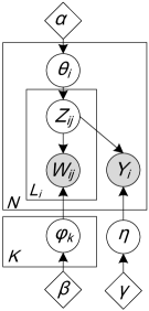
Figure 1: Graphical models of (a) LDA [36]; (b) logistic-normal topic model [34]; and (c) supervised LDA.

A popular Bayesian model that explores such conjugacy is latent Dirichlet allocation (LDA) [36], as illustrated in Fig. 1(a). LDA posits that each document $\mathbf{w}_{i}$ is an admixture of a set of $K$ topics, of which each topic $\boldsymbol{\psi}_{k}$ is a unigram distribution over a given vocabulary. The generative process is as follows:

1. draw $K$ topics $\boldsymbol{\psi}_{k}\sim\textrm{Dir}(\boldsymbol{\beta})$

2. for each document $i\in[N]$:

   1. draw a topic mixing vector $\boldsymbol{\theta}_{i}\sim\textrm{Dir}(\boldsymbol{\alpha})$

   2. for each word $j\in[L_{i}]$ in document $i$:

      1. draw a topic assignment $z_{ij}\sim\textrm{Multi}(\boldsymbol{\theta}_{i})$

      2. draw a word $w_{ij}\sim\textrm{Multi}(\boldsymbol{\psi}_{z_{ij}})$.

LDA has been popular in many applications. However, a conjugate prior can be restrictive. For example, the Dirichlet distribution does not impose correlation between different parameters, except the normalization constraint. In order to obtain more flexible models, a non-conjugate prior can be chosen.

Example 2: Logistic-Normal Prior A logistic-normal distribution [12] provides one way to impose correlation structure among the multiple dimensions of $\boldsymbol{\theta}$. It is defined as follows:

$$\boldsymbol{\eta}\sim\mathcal{N}(\boldsymbol{\mu},\Sigma),\leavevmode\nobreak\ \theta_{k}=\frac{e^{\eta_{k}}}{\sum_{j}e^{\eta_{j}}}.$$ (13)

This prior has been used to develop correlated topic models (or logistic-normal topic models) [34], which can infer the correlation structure among topics. However, the flexibility pays cost on computation, needing scalable algorithms to learn large topic graphs [47].

3 Big Bayesian Learning

Though much more emphasis in big Bayesian learning has been put on scalable algorithms and systems, substantial advances have been made on adaptive and flexible Bayesian methods. This section reviews nonparametric Bayesian methods for adaptively inferring model complexity and regularized Bayesian inference for improving the flexibility via posterior regularization, while leaving the large part of scalable algorithms and systems to next sections.

3.1 Nonparametric Bayesian Methods

For parametric Bayesian models, the parameter space is pre-specified. No matter how the data changes, the number of parameters is fixed. This restriction may cause limitations on model capacity, especially for big data applications, where it may be difficult or even counter-productive to fix the number of parameters a priori. For example, a Gaussian mixture model with a fixed number of clusters may fit the given data set well; however, it may be sub-optimal to use the same number of clusters if more data comes under a slightly changed distribution. It would be ideal if the clustering models can figure out the unknown number of clusters automatically. Similar requirements on automatical model selection exist in feature representation learning [29] or factor analysis, where we would like the models to automatically figure out the dimension of latent features (or factors) and maybe also the topological structure among features (or factors) at different abstraction levels [8].

Nonparametric Bayesian (NPB) methods provide an elegant solution to such needs on automatic adaptation of model capacity when learning a single model. Such adaptivity is obtained by defining stochastic processes on rich measure spaces. Classical examples include Dirichlet process (DP), Indian buffet process (IBP), and Gaussian process (GP). Below, we briefly review DP and IBP. We refer the readers to the articles [73, 71, 133] for a nice overview and the textbook [84] for a comprehensive treatment.

3.1.1 Dirichlet Process

A DP defines the distribution of random measures. It was first developed in [64]. Specifically, a DP is parameterized by a concentration parameter $\alpha>0$ and a base distribution $G_{0}$ over a measure space $\Omega$. A random variable drawn from a DP, $G\sim\mathcal{DP}(\alpha,G_{0})$, is itself a distribution over $\Omega$. It was shown that the random distributions drawn from a DP are discrete almost surely, that is, they place the probability mass on a countably infinite collection of atoms, i.e.,

$$G=\sum_{k=1}^{\infty}\pi_{k}\delta_{\theta_{k}},$$ (14)

where $\theta_{k}$ is the value (or location) of the $k$th atom independently drawn from the base distribution $G_{0}$ and $\pi_{k}$ is the probability assigned to the $k$th atom. Sethuraman [162] provided a constructive definition of $\pi_{k}$ based on a stick-breaking process as illustrated in Fig. 2(a). Consider a stick with unit length. We break the stick into an infinite number of segments $\pi_{k}$ by the following process with $\nu_{k}\sim\textrm{Beta}(1,\alpha)$:

$$\pi_{1}=\nu_{1},\leavevmode\nobreak\ \leavevmode\nobreak\ \pi_{k}=\nu_{k}\prod_{j=1}^{k-1}(1-\nu_{j}),\leavevmode\nobreak\ k=2,3,\dots,\infty.$$ (15)

That is, we first choose a beta variable $\nu_{1}$ and break $\nu_{1}$ of the stick. Then, for the remaining segment, we draw another beta variable and break off that proportion of the remainder of the stick. Such a representation of DP provides insights for developing variational approximate inference algorithms [33].

DP is closely related to the Chinese restaurant process (CRP) [146], which defines a distribution over infinite partitions of integers. CRP derives its name from a metaphor: Image a restaurant with an infinite number of tables and a sequence of customers entering the restaurant and sitting down. The first customer sits at the first table. For each of the subsequent customers, she sits at each of the occupied tables with a probability proportional to the number of previous customers sitting there, and at the next unoccupied table with a probability proportional to $\alpha$. In this process, the assignment of customers to tables defines a random partition. In fact, if we repeatedly draw a set of samples from $G$, that is, $\boldsymbol{\theta}_{i}\sim G,\leavevmode\nobreak\ i\in[N]$, then it was shown that the joint distribution of $\boldsymbol{\theta}_{1:N}$

$$p(\boldsymbol{\theta}_{1},\dots,\boldsymbol{\theta}_{N}|\alpha,G_{0})=\int\left(\prod_{i=1}^{N}p(\boldsymbol{\theta}_{i}|G)\right)\mathrm{d}P(G|\alpha,G_{0})$$

exists a clustering property, that is, the $\boldsymbol{\theta}_{i}$s will share repeated values with a non-zero probability. These shared values define a partition of the integers from 1 to $N$, and the distribution of this partition is a CRP with parameter $\alpha$. Therefore, DP is the de Finetti mixing distribution of CRP.

Antoniak [18] first developed DP mixture models by adding a data generating step, that is, $\mathbf{x}_{i}\sim p(\mathbf{x}|\boldsymbol{\theta}_{i}),\leavevmode\nobreak\ i\in[N].$ Again, marginalizing out the random distribution $G$, the DP mixture reduces to a CRP mixture, which enjoys nice Gibbs sampling algorithms [134]. For DP mixtures, a slice sampler [135] has been developed [180], which transforms the infinite sum in Eq. (14) into a finite sum conditioned on some uniformly distributed auxiliary variable.

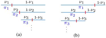
Figure 2: The stick-breaking process for: (a) DP; (b) IBP.

3.1.2 Indian Buffet Process

A mixture model assumes that each data is assigned to one single component. Latent factor models weaken this assumption by associating each data with some or all of the components. When the number of components is smaller than the feature dimension, latent factor models provide dimensionality reduction. Popular examples include factor analysis, principal component analysis and independent component analysis. The general assumption of a latent factor model is that the observed data $\mathbf{x}\in\mathbb{R}^{P}$ is generated by a noisy weighted combination of latent factors, that is,

$$\mathbf{x}_{i}=W\mathbf{z}_{i}+\epsilon_{i},$$ (16)

where $W$ is a $P\times K$ factor loading matrix, with element $W_{mk}$ expressing how latent factor $k$ influences the observation dimension $m$; $\mathbf{z}_{i}$ is a $K$-dimensional vector expressing the activity of each factor; and $\epsilon_{i}$ is a vector of independent noise terms (usually Gassian noise). In the above models, the number of factors $K$ is assumed to be known. Indian buffet process (IBP) [79] provides a nonparametric Bayesian variant of latent factor models and it allows the number of factors to grow as more data are observed.

Consider binary factors for simplicity. Putting the latent factors of $N$ data points in a matrix $Z$, of which the $i$th row is $\mathbf{z}_{i}$. IBP defines a process over the space of binary matrixes with an unbounded number of columns. IBP derives its name from a similar metaphor as CRP. Image a buffet with an infinite number of dishes (factors) arranged in a line and a sequence of customers choosing the dishes. Let $z_{ik}$ denote whether customer $i$ chooses dish $k$. Then, the first customer chooses $K_{1}$ dishes, where $K_{1}\sim\textrm{Poisson}(\alpha)$; and the subsequent customer $n\leavevmode\nobreak\ (>1)$ chooses:

1. each of the previously sampled dishes with probability $m_{k}/n$, where $m_{k}$ is the number of customers who have chosen dish $k$;

2. $K_{i}$ additional dishes, where $K_{i}\sim\textrm{Poisson}(\alpha/n)$.

IBP plays the same role for latent factor models that CRP plays for mixture models, allowing an unbounded number of latent factors. Analogous to the role that DP is the de Finetti mixing distribution of CRP, the de Finetti mixing distribution underlying IBP is a Beta process [175]. IBP also admits a stick-breaking representation [171] as shown in Fig. 2(b), where the stick lengths are defined as

$$\nu_{k}\sim\textrm{Beta}(\alpha,1),\leavevmode\nobreak\ \leavevmode\nobreak\ \pi_{k}=\prod_{j=1}^{k}\nu_{j},\leavevmode\nobreak\ \leavevmode\nobreak\ k=1,2,\dots,\infty.$$ (17)

Note that unlike the stick-breaking representation of DP, where the stick lengths sum to 1, the stick lengths here need not sum to 1. Such a representation has lead to the developments of Monte Carlo [171] as well as variational approximation inference algorithms [58].

3.1.3 Gaussian Process

Kernel machines (e.g., support vector machines) [87] represent an important class of methods in machine learning and has received extensive attention. Gaussian processes (GPs) provide a principled, practical, probabilistic approach to learning in kernel machines. A Gaussian process is defined on the space of continuous functions [150]. In machine learning, the prime use of GPs is to learn the unknown mapping function from inputs to outputs for supervised learning.

Take the simple linear regression model as an example. Let $\mathbf{x}\in\mathbb{R}^{M}$ be an input data point and $y\in\mathbb{R}$ be the output. A linear regression model is

$$f(\mathbf{x})=\boldsymbol{\theta}^{\top}\phi(\mathbf{x}),\leavevmode\nobreak\ \leavevmode\nobreak\ y=f(\mathbf{x})+\epsilon,$$

where $\phi(\mathbf{x})$ is a vector of features extracted from $\mathbf{x}$, and $\epsilon$ is an independent noise. For the Gaussian noise, e.g., $\epsilon\sim\mathcal{N}(0,\sigma^{2}I)$, the likelihood of $y$ conditioned on $\mathbf{x}$ is also a Gaussian, that is, $p(y|\mathbf{x},\boldsymbol{\theta})=\mathcal{N}(f(\mathbf{x}),\sigma^{2}I)$. Consider a Bayesian approach, where we put a zero-mean Gaussian prior, $\boldsymbol{\theta}\sim\mathcal{N}(0,\Sigma)$. Given a set of training observations $\mathcal{D}=\{(\mathbf{x}_{i},y_{i})\}_{i=1}^{N}$. Let $X$ be the $M\times N$ design matrix, and $\mathbf{y}$ be the vector of the targets. By Bayes’ theorem, we can easily derive that the posterior is also a Gaussian distribution (see [150] for more details)

$$p(\boldsymbol{\theta}|X,\mathbf{y})=\mathcal{N}\left(\frac{1}{\sigma^{2}}A^{-1}\Phi\mathbf{y},A^{-1}\right),$$ (18)

where $A^{-1}=\sigma^{-2}\Phi\Phi^{\top}+\Sigma^{-1}$ and $\Phi=\phi(X)$. For a test example $\mathbf{x}_{\ast}$, we can also derive that the distribution of the predictive value $f_{\ast}\triangleq f(\mathbf{x}_{\ast})$ is also a Gaussian:

$$p(f_{\ast}|\mathbf{x}_{\ast},X,\mathbf{y})=\mathcal{N}\left(\frac{1}{\sigma^{2}}\phi_{\ast}^{\top}A^{-1}\Phi\mathbf{y},\phi_{\ast}^{\top}A^{-1}\phi_{\ast}\right),$$ (19)

where $\phi_{\ast}\triangleq\phi(\mathbf{x}_{\ast})$. In some equivalent form, the Gaussian mean and covariance only involve the inner products in input space. Therefore, the kernel trick can be explored in such models, which avoids the explicit evaluation of the feature vectors.

The above Bayesian linear regression model is a very simple example of Gaussian processes. In the most general form, Gaussian processes define a stochastic process over functions $f(\mathbf{x})$. A GP is characterized by a mean function $m(\mathbf{x})$ and a covariance function $\kappa(\mathbf{x},\mathbf{x}^{\prime})$, denoted by $f(\mathbf{x})\sim\mathcal{GP}(m(\mathbf{x}),\kappa(\mathbf{x},\mathbf{x}^{\prime})$. Given any finite set of observations $\mathbf{x}_{1},\dots,\mathbf{x}_{n}$, the function values $(f(\mathbf{x}_{1}),\dots,f(\mathbf{x}_{n}))$ follow a multivariate Gaussian distribution with mean $(m(\mathbf{x}_{1}),\dots,m(\mathbf{x}_{n}))$ and covariance $K:\leavevmode\nobreak\ K(i,j)=\kappa(\mathbf{x}_{i},\mathbf{x}_{j})$. The above definition with any finite collection of function values guarantee to define a stochastic process (i.e., Gaussian process), by examining the consistency requirement of the Kolmogorov extension theorem.

Gaussian processes have also been used in classification tasks, where the likelihood is often non-conjugate to the Gaussian process prior, therefore requiring approximate inference algorithms, including both variational and Monte Carlo methods. Other research has considered Gaussian process latent variable models (GP-LVM) [107].

3.1.4 Extensions

To meet the flexibility and adaptivity requirements of big learning, many recent advances have been made on developing sophisticated NPB methods for modeling various types of data, including grouped data, spatial data, time series, and networks.

Hierarchical models are natural tools to describe grouped data, e.g., documents from different source domains. Hierarchical Dirichlet process (HDP) [172] and hierarchical Beta process [175] have been developed, allowing an infinite number of latent components to be shared by multiple domains. The work [8] presents a cascading IBP (CIBP) to learn the topological structure of multiple layers of latent features, including the number of layers, the number of hidden units at each layer, the connection structure between units at neighboring layers, and the activation function of hidden units. The recent work [52] presents an extended CIBP process to generate connections between non-consecutive layers.

Another dimension of the extensions concerns modeling the dependencies between observations in a time series. For example, DP has been used to develop the infinite hidden Markov models [23], which posit the same sequential structure as in the hidden Markov models, but allowing an infinite number of latent classes. In [172], it was shown that iHMM is a special case of HDP. The recent work [198] presents a max-margin training of iHMMs under the regularized Bayesian framework, as will be reviewed shortly.

Finally, for spatial data, modeling dependency between nearby data points is important. Recent extensions of Bayesian nonparametric methods include the dependent Dirichlet process [120], spatial Dirichlet process [59], distance dependent CRP [32], dependent IBP [188], and distance dependent IBP [70]. For network data analysis (e.g., social networks, biological networks, and citation networks), recent extensions include the nonparametric Bayesian relational latent feature models for link prediction [128, 200], which adopt IBP to allow for an unbounded number of latent features, and the nonparametric mixed membership stochastic block models for community discovery [77, 98], which use HDP to allow mixed membership in an unbounded number of latent communities.

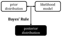
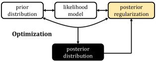
Figure 3: (a) Bayesian inference with the Bayes’ rule; and (b) regularized Bayesian inference (RegBayes) which solves an optimization problem with a posterior regularization term to incorporate rich side information.

3.2 Regularized Bayesian Inference

Regularized Bayesian inference (RegBayes) [203] represents one recent advance that extends the scope of Bayesian methods on incorporating rich side information. Recall that the classic Bayes’ theorem is equivalent to a variational optimization problem as in (2). RegBayes builds on this formulation and defines the generic optimization problem

$$\min_{q(\boldsymbol{\Theta})\in\mathcal{P}}\mathrm{KL}(q(\boldsymbol{\Theta})\|p(\boldsymbol{\Theta}|\mathcal{D}))+c\cdot\Omega(q(\boldsymbol{\Theta});\mathcal{D}),$$ (20)

where $\Omega(q(\boldsymbol{\Theta});\mathcal{D})$ is the posterior regularization term; $c$ is a nonnegative regularization parameter; and $p(\boldsymbol{\Theta}|\mathcal{D})$ is the ordinary Bayesian posterior. Fig. 3 provides a high-level comparison between RegBayes and Bayes’ rule. Several questions need to be answered in order to solve practical problems.

Q: How to define the posterior regularization?

A: In general, posterior regularization can be any informative constraints that are expected to regularize the properties of the posterior distribution. It can be defined as the large-margin constraints to enforce a good prediction accuracy [201], or the logic constraints to incorporate expert knowledge [126], or the sparsity constraints [102].

Example 3: Max-margin LDA Following the paradigm of ordinary Bayes, a supervised topic model is often defined by augmenting the likelihood model. For example, the supervised LDA (sLDA) [35] has a similar structure as LDA (see Fig. 1(c)), but with an additional likelihood $p(y_{d}|\mathbf{z}_{d},\boldsymbol{\eta})$ to describe labels. Such a design can lead to an imbalanced combination of the word likelihood $p(\mathbf{w}_{d}|\mathbf{z}_{d},\boldsymbol{\psi})$ and the label likelihood because a document often has tens or hundreds of words while only one label. The imbalance problem causes unsatisfactory prediction results [204].

To improve the discriminative power of supervised topic models, the max-margin MedLDA has been developed, under the RegBayes framework. Consider binary classification for simplicity. In this case, we have $\boldsymbol{\Theta}=\{\boldsymbol{\theta}_{i},\mathbf{z}_{i},\boldsymbol{\psi}_{k}\}$. Let $f(\boldsymbol{\eta},\mathbf{z}_{i})=\boldsymbol{\eta}^{\top}\bar{\mathbf{z}}_{i}$ be the discriminant function, where $\bar{\mathbf{z}}_{i}$ is the average topic assignments, with $\bar{z}_{i}^{k}=\frac{1}{L_{i}}\sum_{j}{\mathbb{I}}(z_{ij}=k)$. The posterior regularization can be defined in two ways:

Averaging classifier: An averaging classifier makes predictions using the expected discriminant function, that is, $\hat{y}(q)=\textrm{sign}(\mathbb{E}_{q}[f(\boldsymbol{\eta},\mathbf{z})])$. Let $(x)_{+}=\max(0,x)$. Then, the posterior regularization

$$\Omega^{\textrm{Avg}}(q(\boldsymbol{\Theta});\mathcal{D})=\sum_{i=1}^{N}(1-y_{i}\mathbb{E}_{q}[f(\boldsymbol{\eta},\mathbf{z}_{i})])_{+}$$

is an upper bound of the training error, therefore a good surrogate loss for learning. This strategy has been adopted in MedLDA [201].

Gibbs classifier: A Gibbs classifier (or stochastic classifier) randomly draws a sample $(\boldsymbol{\eta},\mathbf{z}_{d})$ from the target posterior $q(\boldsymbol{\Theta})$ and makes predictions using the latent prediction rule, that is, $\hat{y}(\boldsymbol{\eta},\mathbf{z}_{i})=\textrm{sign}f(\boldsymbol{\eta},\mathbf{z}_{i})$. Then, the posterior regularization is defined as

$$\Omega^{\textrm{Gibbs}}(q(\boldsymbol{\Theta});\mathcal{D})=\mathbb{E}_{q}\left[\sum_{i=1}^{N}(1-y_{i}f(\boldsymbol{\eta},\mathbf{z}_{i}))_{+}\right].$$

This strategy has been adopted to develop Gibbs MedLDA [202].

The two strategies are closely related, e.g., we can show that $\Omega^{\textrm{Gibbs}}(q(\boldsymbol{\Theta}))$ is an upper bound of $\Omega^{\textrm{Avg}}(q(\boldsymbol{\Theta}))$. The formulation with a Gibbs classifier can lead to a scalable Gibbs sampler by using data augmentation techniques [205]. If a logistic log-loss is adopted to define the posterior regularization, an improved sLDA model can be developed to address the imbalance issue and lead to significantly more accurate predictions [204].

Q: What is the relationship between prior, likelihood, and posterior regularization?

A: Though the three parts are closely connected, there are some key differences. First, prior is chosen before seeing data, while both likelihood and posterior regularization depend on the data. Second, different from the likelihood, which is restricted to be a normalized distribution, no constraints are imposed on the posterior regularization. Therefore, posterior regularization is much more flexible than prior or likelihood. In fact, it can be shown that (1) putting constraints on priors is a special case of posterior regularization, where the regularization term does not depend on data; and (2) RegBayes can be more flexible than standard Bayes’ rule, that is, there exists some RegBayes posterior distributions that are not achievable by the Bayes’ rule [203].

Q: How to solve the optimization problem?

A: The posterior regularization term affects the difficulty of solving problem (20). When the regularization term is a convex functional of $q(\boldsymbol{\Theta})$, which is common in many applications such as the above max-margin formulations, the optimal solution can be characterized in a general from via convex duality theory [203]. When the regularization term is non-convex, a generalized representation theorem can also be derived, but requires more effects on dealing with the non-convexity [102].

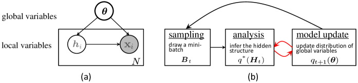
Figure 4: (a) The general structure of Bayesian latent variable models, where $\mathbf{h}_{i}$ denotes the local latent variables for each data $i$; (b) the process of stochastic variational inference, where the red arrows denote that in practice we may need multiple iterations between “analysis” and “model update” to have fast convergence.

4 Scalable Algorithms

To deal with big data, the posterior inference algorithms should be scalable. Significant advances have been made in two aspects: (1) using random sampling to do stochastic or online Bayesian inference; and (2) using multi-core and multi-machine architectures to do parallel and distributed Bayesian inference.

4.1 Stochastic Algorithms

In Big Learning, the intriguing results of [38] suggest that an algorithm as simple as stochastic gradient descent (SGD) can be optimally efficient in terms of “number of bits learned per unit of computation”. For Bayesian models, both stochastic variational and stochastic Monte Carlo methods have been developed to explore the redundancy of data relative to a model by subsampling data examples for every update and reasoning about the uncertainty created in this process [184]. We overview each type in turn.

4.1.1 Stochastic Variational Methods

As we have stated in Section 2.3.1, variational methods solve an optimization problem to find the best approximate distribution to the target posterior. When the variational distribution is characterized in some parametric form, this problem can be solved with stochastic gradient descent (SGD) methods [40] or the adaptive SGD [60]. A SGD method randomly draws a subset $B_{t}$ and updates the variational parameters using the estimated gradients, that is,

$$\boldsymbol{\phi}_{t+1}\leftarrow\boldsymbol{\phi}_{t}+\epsilon_{t}\left(\nabla_{\boldsymbol{\phi}}\mathrm{KL}(q\|p_{0}(\boldsymbol{\theta}))-\nabla_{\boldsymbol{\phi}}\mathbb{E}_{q}[\log p(\mathcal{D}|\boldsymbol{\theta})]\right),$$

where the full data gradient is approximated as

$$\nabla_{\boldsymbol{\phi}}\mathbb{E}_{q}[\log p(\mathcal{D}|\boldsymbol{\theta})]\approx\frac{N}{|B_{t}|}\sum_{i\in B_{t}}\nabla_{\boldsymbol{\phi}}\mathbb{E}_{q}[\log p(\mathbf{x}_{i}|\boldsymbol{\theta})],$$ (21)

and $\epsilon_{t}$ is a learning rate. If the noisy gradient is an unbiased estimate of the true gradient, the procedure is guaranteed to approach the optimal solution when the learning rate is appropriately set [37].

For Bayesian latent variable models, we need to infer the latent variables when performing the updates. In general, we can group the latent variables into two categories — global variables and local variables. Global variables correspond to the model parameters $\boldsymbol{\theta}$ (e.g., the topics $\boldsymbol{\psi}$ in LDA), while local variables represent some hidden structures of the data (e.g., the topic assignments $\mathbf{z}$ in an LDA with the topic mixing proportions collapsed out). Fig. 4 provides an illustration of such models and the stochastic variational inference, which consists of three steps:

1. randomly draw a mini-batch $B_{t}$ of data samples;

2. infer the local latent variables for each data in $B_{t}$;

3. update the global variables.

However, the standard gradients over the parameters $\boldsymbol{\phi}$ may not be the most informative direction (i.e., the steepest direction) to search for the distribution $q$. A better way is to use natural gradient [14], which is the steepest search direction in a Riemannian manifold space of probability distributions [86]. To reduce the efforts on hand-tuning the learning rate, which often influences the performance much, the work [149] presents an adaptive learning rate while [165] adopts Bayesian optimization to search for good learning rates, both leading to faster convergence. By borrowing the gradient averaging ideas from stochastic optimization, [123] proposes to use smoothed gradients in stochastic variational inference to reduce the variance (by trading-off the bias). Stochastic variational inference methods have been studied for many Bayesian models, such as LDA and hierarchical Dirichlet process [86].

In many cases, the ELBO and its gradient may be intractable to compute due to the intractability of the expectation over variational distributions. Two types of methods are commonly used to address this problem. First, another layer of variational bound is derived by introducing additional variational parameters. This has been used in many examples, such as the logistic-normal topic models [34] and supervised LDA [35]. For such methods, it is important to develop tight variational bounds for specific models [124], which is still an active area. Another type of methods is to use Monte Carlo estimates of the variational bound as well as its gradients. Recent work includes the stochastic approximation scheme with variance reduction [141, 149] and the auto-encoding variational Bayes (AEVB) [99] that learns a neural network (a.k.a recognition model) to represent the variational distribution for continuous latent variables.

Consider the model with one layer of continuous latent variables $\mathbf{h}_{i}$ in Fig. 4 (a). Assume the variational distribution $q_{\boldsymbol{\phi}}(\boldsymbol{\Theta})=q_{\boldsymbol{\phi}}(\boldsymbol{\theta})\prod_{i=1}^{N}q_{\boldsymbol{\phi}}(\mathbf{h}_{i}|\mathbf{x}_{i})$. Let $G_{\boldsymbol{\phi}}(\mathbf{x},\mathbf{h},\boldsymbol{\theta})=\log p(\mathbf{h}|\boldsymbol{\theta})+\log p(\mathbf{x}|\mathbf{h},\boldsymbol{\theta})-\log q_{\boldsymbol{\phi}}(\mathbf{h}|\mathbf{x})$. The ELBO in Eq. (2) can be written as

$$\mathcal{L}(\boldsymbol{\phi};\mathcal{D})=\mathbb{E}_{q}\left[\log p_{0}(\boldsymbol{\theta})+\!\sum_{i}\!G_{\boldsymbol{\phi}}(\mathbf{x}_{i},\mathbf{h}_{i},\boldsymbol{\theta})-\log q_{\boldsymbol{\phi}}(\boldsymbol{\theta})\right].$$

By using the equality $\nabla_{\boldsymbol{\phi}}q_{\boldsymbol{\phi}}(\boldsymbol{\Theta})=q_{\boldsymbol{\phi}}(\boldsymbol{\Theta})\nabla_{\boldsymbol{\phi}}\log q_{\boldsymbol{\phi}}(\boldsymbol{\Theta})$, it can be shown that the gradient is

$$\nabla_{\boldsymbol{\phi}}\mathcal{L}=\mathbb{E}_{q}\left[(\log p(\boldsymbol{\Theta},\mathcal{D})-\log q_{\boldsymbol{\phi}}(\boldsymbol{\Theta}))\nabla_{\boldsymbol{\phi}}\log q_{\boldsymbol{\phi}}(\boldsymbol{\Theta})\right].$$

A naive Monte Carlo estimate of the gradient is

$$\nabla_{\boldsymbol{\phi}}\mathcal{L}\approx\frac{1}{L}\sum_{l=1}^{L}\left[(\log p(\boldsymbol{\Theta}^{l},\mathcal{D})-\log q_{\boldsymbol{\phi}}(\boldsymbol{\Theta}^{l}))\nabla_{\boldsymbol{\phi}}\log q_{\boldsymbol{\phi}}(\boldsymbol{\Theta}^{l})\right],$$

where $\boldsymbol{\Theta}^{l}\sim q_{\boldsymbol{\phi}}(\boldsymbol{\Theta})$. Note that the sampling and the gradient $\nabla_{\boldsymbol{\phi}}\log q_{\boldsymbol{\phi}}(\boldsymbol{\Theta}^{l})$ only depend on the variational distribution, not the underlying model. However, the variance of such an estimate can be too large to be useful. In practice, effective variance reduction techniques are needed [141, 149].

For continuous $\mathbf{h}$, a reparameterization of the samples $\mathbf{h}\sim q_{\boldsymbol{\phi}}(\mathbf{h}|\mathbf{x})$ can be derived using a differentiable transformation $g_{\boldsymbol{\phi}}(\boldsymbol{\epsilon},\mathbf{x})$ of a noise variable $\boldsymbol{\epsilon}$:

$$\mathbf{h}=g_{\boldsymbol{\phi}}(\boldsymbol{\epsilon},\mathbf{x}),\leavevmode\nobreak\ \textrm{where}\leavevmode\nobreak\ \boldsymbol{\epsilon}\sim p(\boldsymbol{\epsilon}).$$ (22)

This is known as non-centered parameterization (NCP) in statistics [142], while the original representation is known as centered parameterization (CP). A similar NCP reparameterization exists for the continuous $\boldsymbol{\theta}$:

$$\boldsymbol{\theta}=f_{\boldsymbol{\phi}}(\boldsymbol{\zeta}),\leavevmode\nobreak\ \textrm{where}\leavevmode\nobreak\ \boldsymbol{\zeta}\sim p(\boldsymbol{\zeta}).$$ (23)

Given a minibatch of data points $B_{t}$, we define $F_{\boldsymbol{\phi}}(\{\mathbf{x}_{i},\mathbf{h}_{i}\}_{i\in B_{t}},\boldsymbol{\theta})=\frac{N}{|B_{t}|}\sum_{i\in B_{t}}G_{\boldsymbol{\phi}}(\mathbf{x}_{i},\mathbf{h}_{i},\boldsymbol{\theta})+\log p_{0}(\boldsymbol{\theta})-\log q_{\boldsymbol{\phi}}(\boldsymbol{\theta})$. Then, the Monte Carlo estimate of the variational lower bound is

$$\mathcal{L}(\boldsymbol{\phi};\mathcal{D})\approx\frac{1}{L}\sum_{l=1}^{L}F_{\boldsymbol{\phi}}\left(\{\mathbf{x}_{i},g_{\boldsymbol{\phi}}(\boldsymbol{\epsilon}^{l},\mathbf{x}_{i})\}_{i\in B_{t}},f_{\boldsymbol{\phi}}(\boldsymbol{\zeta}^{l})\right),$$ (24)

where $\boldsymbol{\epsilon}^{l}\sim p(\boldsymbol{\epsilon})$ and $\boldsymbol{\zeta}^{l}\sim p(\boldsymbol{\zeta})$. This stochastic estimate can be maximized via gradient ascent methods.

It has been analyzed that CP and NCP possess complimentary strengths [142], in the sense that NCP is likely to work when CP does not and conversely. An accompany paper [100] to AEVB analyzes the conditions for gradient-based samplers (e.g., HMC) whether NCP can be effective or ineffective in reducing posterior dependencies; and it suggests to use the interleaving strategy between centered and non-centered parameterization as previously studied in [195]. AEVB has been extended to learn deep generative models [152] using the similar reparameterization trick on continuous latent variables. However, AEVB cannot be directly applied to deal with discrete variables. In contrast, the work [131] presents a sophisticated method to reduce the variance of the naive Monte Carlo estimate for deep autoregressive models; thus it is applicable to both continuous and discrete latent variables.

4.1.2 Stochastic Monte Carlo Methods

The existing stochastic Monte Carlo methods can be generally grouped into three categories, namely, stochastic gradient-based methods, the methods using approximate MH test with randomly sampled mini-batches, and data augmentation.

Stochastic Gradient: The idea of using gradient information to improve the mixing rates has been systematically studied in various MC methods, including Langevin dynamics and Hamiltanian dynamics [136]. For example, the Langevin dynamics is an MCMC method that produces samples from the posterior by means of gradient updates plus Gaussian noise, resulting in a proposal distribution $p(\boldsymbol{\theta}_{t+1}|\boldsymbol{\theta}_{t})$ by the following equation:

$$\boldsymbol{\theta}_{t+1}=\boldsymbol{\theta}_{t}+\frac{\epsilon_{t}}{2}\left(\nabla_{\boldsymbol{\theta}}\log p_{0}(\boldsymbol{\theta})+\nabla_{\boldsymbol{\theta}}\log p(\mathcal{D}|\boldsymbol{\theta})\right)+\zeta_{t},$$ (25)

where $\zeta_{t}\sim\mathcal{N}(0,\epsilon_{t}I)$ is an isotropic Gaussian noise and $\log p(\mathcal{D}|\boldsymbol{\theta})=\sum_{i}\log p(\mathbf{x}_{i}|\boldsymbol{\theta})$ is the log-likelihood of the full data set. The mean of the proposal distribution is in the direction of increasing log posterior due to the gradient, while the Gaussian noise will prevent the samples from collapsing to a single maximum. A Metropolis-Hastings correction step is required to correct for discretisation error [155].

The stochastic ideas have been successfully explored in these methods to develop efficient stochastic Monte Carlo methods, including stochastic gradient Langevin dynamics (SGLD) [185] and stochastic gradient Hamiltonian dynamics (SGHD) [48]. For example, SGLD replaces the calculation of the gradient over the full data set, with a stochastic approximation based on a subset of data. Let $B_{t}$ be the subset of data points uniformly sampled from the full data set at iteration $t$. Then, the gradient is approximated as:

$$\nabla_{\boldsymbol{\theta}}\log p(\mathcal{D}|\boldsymbol{\theta})\approx\frac{N}{|B_{t}|}\sum_{i\in B_{t}}\nabla_{\boldsymbol{\theta}}\log p(\mathbf{x}_{i}|\boldsymbol{\theta}).$$ (26)

Note that SGLD doesn’t use a MH correction step, as calculating the acceptance probability requires use of the full data set. Convergence to the posterior is still guaranteed if the step sizes are annealed to zero at a certain rate, as rigorously justified in [145, 173].

To further improve the mixing rates, the stochastic gradient Fisher scoring method [10] was developed, which represents an extension of the Fisher scoring method based on stochastic gradients [159] by incorporating randomness in a subsampling process. Similarly, exploring the Riemannian manifold structure leads to the development of stochastic gradient Riemannian Langevin dynamics (SGRLD) [143], which performs SGLD on the probability simplex space.

Approximate MH Test: Another category of stochastic Monte Carlo methods rely on approximate MH test using randomly sampled subset of data points, since an exact calculation of the MH test in Eq. (10) scales linearly to the data size, which is prohibitive for large-scale data sets. For example, the work [101] presents an approximate MH rule via sequential hypothesis testing, which allows us to accept or reject samples with high confidence using only a fraction of the data required for the exact MH rule. The systematic bias and its tradeoff with variance were theoretically analyzed. Specifically, it is based on the observation that the MH test rule in Eq. (10) can be equivalently written as follows:

1. Draw $\gamma\sim\textrm{Uniform}[0,1]$ and compute:

   $$\mu_{0} = \frac{1}{N}\log\left[\gamma\frac{p_{0}(\boldsymbol{\Theta}_{t})q(\boldsymbol{\Theta}^{\prime}|\boldsymbol{\Theta}_{t})}{p_{0}(\boldsymbol{\Theta}^{\prime})q(\boldsymbol{\Theta}_{t}|\boldsymbol{\Theta}^{\prime})}\right]$$

   $$\mu = \frac{1}{N}\sum_{i=1}^{N}\ell_{i},\leavevmode\nobreak\ \textrm{where}\leavevmode\nobreak\ \ell_{i}=\log\frac{p(\mathbf{x}_{i}|\boldsymbol{\Theta}^{\prime})}{p(\mathbf{x}_{i}|\boldsymbol{\Theta}_{t})};$$

2. If $\mu>\mu_{0}$ set $\boldsymbol{\Theta}_{t+1}\leftarrow\boldsymbol{\Theta}^{\prime}$; otherwise $\boldsymbol{\Theta}_{t+1}\leftarrow\boldsymbol{\Theta}_{t}$.

Note that $\mu_{0}$ is independent of the data set, thus can be easily calculated. This reformulation of the MH test makes it very easy to frame it as a statistical hypothesis test, that is, given $\mu_{0}$ and a set of samples $\{\ell_{t_{1}},\dots,\ell_{t_{n}}\}$ drawn without replacement from the population $\{\ell_{1},\dots,\ell_{N}\}$, can we decide whether the population mean $\mu$ is greater than or less than the threshold $\mu_{0}$? Such a test can be done by increasing the cardinality of the subset until a prescribed confidence level is reached. The MH test with approximate confidence intervals can be combined with the above stochastic gradient methods (e.g., SGLD) to correct their bias. The similar sequential testing ideas can be applied to Gibbs sampling, as discussed in [101].

Under the similar setting of approximate MH test with subsets of data, the work [21] derives a new stopping rule based on some concentration bounds (e.g., the empirical Bernstein bound [22]), which leads to an adaptive sampling strategy with theoretical guarantees on the total variational norm between the approximate MH kernel and the target distribution of MH applied to the full data set.

Data Augmentation: The work [121] presents a Firefly Monte Carlo (FlyMC) method, which is guaranteed to converge to the true target posterior. FlyMC relies on a novel data augmentation formulation [61]. Specifically, let $z_{i}$ be a binary variable, indicating whether data $i$ is active or not, and $B_{i}(\boldsymbol{\Theta})$ be a strictly positive lower bound of the $i$th likelihood: $0<B_{i}(\boldsymbol{\Theta})<L_{i}(\boldsymbol{\Theta})\triangleq p(\mathbf{x}_{i}|\boldsymbol{\Theta})$. Then, the target posterior $p(\boldsymbol{\Theta}|\mathcal{D})$ is the marginal of the complete posterior with the augmented variables $\mathbf{Z}=\{z_{i}\}_{i=1}^{N}$:

$$p(\boldsymbol{\Theta},\mathbf{Z}|\mathcal{D})\propto p_{0}(\boldsymbol{\Theta})\prod_{i=1}^{N}p(\mathbf{x}_{i}|\boldsymbol{\Theta})p(z_{i}|\mathbf{x}_{i},\boldsymbol{\Theta}),$$ (27)

where $p(z_{i}|\mathbf{x}_{i},\boldsymbol{\Theta})=(1-\gamma_{i})^{z_{i}}\gamma_{i}^{(1-z_{i})}$ and $\gamma_{i}=B_{i}(\boldsymbol{\Theta})/L_{i}(\boldsymbol{\Theta})$. Then, we can construct a Markov chain for the complete posterior by alternating between updates of $\boldsymbol{\Theta}$ conditioned on $\mathbf{Z}$, which can be done with any conventional MCMC algorithm, and updates of $\mathbf{Z}$ conditioned on $\boldsymbol{\Theta}$, which can also been efficiently done as we only need to re-calculate the likelihoods of the data points with active $z$ variables, thus effectively using a random subset of data points in each iteration of the MC methods.

4.2 Streaming Algorithms

We can see that both (21) and (26) need to know the data size $N$, which renders them unsuitable for learning with streaming data, where data comes in small batches without an explicit bound on the total number as times goes along, e.g., tracking an aircraft using radar measurements. This conflicts with the sequential nature of the Bayesian updating procedure. Specifically, let $B_{t}$ be the small batch at time $t$. Given the posterior at time $t$, $p_{t}(\boldsymbol{\Theta}):=p(\boldsymbol{\Theta}|B_{1},\dots,B_{t})$, the posterior distribution at time $t+1$ is

$$p_{t+1}(\boldsymbol{\Theta}):=p(\boldsymbol{\Theta}|B_{1},\dots,B_{t+1})=\frac{p_{t}(\boldsymbol{\Theta})p(B_{t+1}|\boldsymbol{\Theta})}{p(B_{1},\dots,B_{t+1})}.$$ (28)

In other words, the posterior at time $t$ is actually playing the role of a prior for the data at time $t+1$ for the Bayesian updating. Under the variational formulation of Bayes’ rule, streaming RegBayes [163] can naturally be defined as solving:

$$\min_{q(\boldsymbol{\Theta})\in\mathcal{P}}\mathrm{KL}(q(\boldsymbol{\Theta})\|p_{t}(\boldsymbol{\Theta}))+c\cdot\Omega(q(\boldsymbol{\Theta});B_{t+1}),$$ (29)

whose streaming update rule can be derived via convex analysis under a quite general setting.

The sequential updating procedure is perfectly suitable for online learning with data streams, where a revisit to each data point is not allowed. However, one challenge remains on evaluating the posteriors. If the prior is conjugate to the likelihood model (e.g., a linear Gaussian state-space model) or the state space is discrete (e.g., hidden Markov models [148, 161]), then the sequential updating rule can be done analytically, for example, Kalman filters [96]. In contrast, many complex Bayesian models (e.g., the models involving non-Gaussianity, non-linearity and high-dimensionality) do not have closed-form expression of the posteriors. Therefore, it is computationally intractable to do the sequential update.

4.2.1 Streaming Variational Methods

Various effects have been made to develop streaming variational Bayesian (SVB) methods [42]. Specifically, let $\mathcal{A}$ be a variational algorithm that calculates the approximate posterior $q$: $q(\boldsymbol{\Theta})=\mathcal{A}(p(\Theta);B)$. Then, setting $q_{0}(\boldsymbol{\Theta})=p_{0}(\boldsymbol{\Theta})$, one way to recursively compute an approximation to the posterior is

$$p(\boldsymbol{\Theta}|B_{1},\dots,B_{t+1})\approx q_{t+1}(\boldsymbol{\Theta})=\mathcal{A}(q_{t}(\boldsymbol{\Theta}),B_{t+1}).$$ (30)

Under the exponential family assumption of $q$, the streaming update rule has some analytical form.

The streaming RegBayes [163] provides a Bayesian generalization of online passive-aggressive (PA) learning [50], when the posterior regularization term is defined via the max-margin principle. The resulting online Bayesian passive-aggressive (BayesPA) learning adopts a similar streaming variational update to learn max-margin classifiers (e.g., SVMs) in the presence of latent structures (e.g., latent topic representations). Compared to the ordinary PA, BayesPA is more flexible on modeling complex data. For example, BayesPA can discover latent structures via a hierarchical Bayesian treatment as well as allowing for nonparametric Bayesian inference to resolve the complexity of latent components (e.g., using a HDP topic model to resolve the unknown number of topics).

4.2.2 Streaming Monte Carlo Methods

Sequential Monte Carlo (SMC) methods [15, 116, 19] provide simulation-based methods to approximate the posteriors for online Bayesian inference. SMC methods rely on resampling and propagating samples over time with a large number of particles. A standard SMC method would require the full data to be stored for expensive particle rejuvenation to protect particles against degeneracy, leading to an increased storage and processing bottleneck as more data are accrued. For simple conjugate models, such as linear Gaussian state-space models, efficient updating equations can be derived using methods like Kalman filters. For a broader class of models, assumed density filtering (ADF) [106, 140] was developed to extend the computational tractability. Basically, ADF approximates the posterior distribution with a simple conjugate family, leading to approximate online posterior tracking. Recent improvements on SMC methods include the conditional density filtering (C-DF) method [81], which extends Gibbs sampling to streaming data. C-DF sequentially draws samples from an approximate posterior distribution conditioned on surrogate conditional sufficient statistics, which are approximations to the conditional sufficient statistics using sequential samples or point estimates for parameters along with the data. C-DF requires only data at the current time and produces a provably good approximation to the target posterior.

4.3 Distributed Algorithms

Recent progress has been made on both distributed variational and distributed Monte Carlo methods.

4.3.1 Distributed Variational Methods

If the variational distribution is in some parametric family (e.g., the exponential family), the variational problem can be solved with generic optimization methods. Therefore, the broad literature on distributed optimization [39] provides rich tools for distributed variational inference. However, the disadvantage of a generic solver is that it may fail to explore the structure of Bayesian inference.

First, many Bayesian models have a nature hierarchy, which encodes rich conditional independence structures that can be explored for efficient algorithms, e.g., the distributed variational algorithm for LDA [197]. Second, the inference procedure with Bayes’ rule is intrinsically parallelizable. Suppose the data $\mathcal{D}$ is split into non-overlapping batches (often called shards), $B_{1}$, $\dots$, $B_{M}$. Then, the Bayes posterior $p(\boldsymbol{\Theta}|\mathcal{D})=\frac{p_{0}(\boldsymbol{\Theta})\prod_{i=1}^{M}p(B_{i}|\boldsymbol{\Theta})}{p(\mathcal{D})}$ can be expressed as

$$p(\boldsymbol{\Theta}|\mathcal{D})=\frac{1}{C}\!\prod_{i=1}^{M}\frac{p_{0}(\boldsymbol{\Theta})^{\frac{1}{M}}p(B_{i}|\boldsymbol{\Theta})}{p(B_{i})}=\frac{1}{C}\!\prod_{i=1}^{M}p(\boldsymbol{\Theta}|B_{i}),$$ (31)

where $C=\frac{p(\mathcal{D})}{\prod_{i=1}^{M}p(B_{i})}$. Now, the question is how to calculate the local posteriors (or subset posteriors) $p(\boldsymbol{\Theta}|B_{i})$ as well as the normalization factor. The work [42] explores this idea and presents a distributed variational Bayesian method, which approximates the local posterior with an algorithm $\mathcal{A}$, that is, $p(\boldsymbol{\Theta}|B_{i})\approx\mathcal{A}\left(p_{0}(\boldsymbol{\Theta})^{1/M},B_{i}\right).$ Under the exponential family assumption of the prior and the approximate local posteriors, the global posterior can be (approximately) calculated via density product. However, the parametric assumptions may not be reasonable, and the mean-field assumptions can get the marginal distributions right but not the joint distribution.

4.3.2 Distributed Monte Carlo Methods

For MC methods, if independent samples can be directly drawn from the posterior or some proposals (e.g., using importance sampling), it will be straightforward to parallelize, e.g., by running multiple independent samplers on separate machines and then aggregating the samples [190]. We consider the more challenging cases, where directly sampling from the posterior is intractable and MCMC methods are among the natural choices. There are two groups of methods. One is to run multiple MCMC chains in parallel, and the other is to parallelize a single MCMC chain. The “multiple-chain” parallelism is relatively straightforward if each single chain can be efficiently carried out and an appropriate combination strategy is adopted [67, 190]. However, in Big data applications a single Markov chain itself is often prohibitively slow to converge, due to the massive data sizes or extremely high-dimensional sample spaces. Below, we focus on the methods that parallelize a single Markov chain, under three major categories.

Blocking: Methods in this category let each computing unit (e.g., a CPU processor or a GPU core) to perform a part of the computation at each iteration. For example, they independently evaluate the likelihood for each shard across multiple units and combine the local likelihoods with the prior on a master unit to get estimates of the global posterior [168]. Another example is that each computing unit is responsible for updating a part of the state space [186]. These methods involve extensive communications and being problem specific.

In these methods several computing units collaborate to obtain a draw from the posterior. In order to effectively split the likelihood evaluation or the state space update over multiple computing units, it is important to explore the conditional independence (CI) structure of the model. Many hierarchical Bayesian models naturally have the CI structure (e.g., topic models), while some other models need some transformation to introduce CI structures that are appropriate for parallelization [189].

Divide-and-Conquer: Methods in this category avoid extensive communication among machines by running independent MCMC chains on each shard and aggregating samples drawn from local posteriors via a single communication. Aggregating the local samples is the key step, with a lot of recent progress. For example, the consensus Monte Carlo [160] directly combines local samples by a weighted average, which is valid under an implicit Gaussian assumption while lacking of guarantees for non-Gaussian cases; [137] approximates each local posterior with either an explicit Gaussian or a Gaussian-kernel KDE so that combination follows an explicit density product; [181] builds upon the KDE idea one step further by representing the discrete KDE as a continuous Weierstrass transform; and  [129] proposes to calculate the geometric median of local posteriors (or M-posterior), which is provably robust to the presence of outliers. The M-posterior is approximately solved by the Weiszfeld’s algorithm [26] by embedding the local posteriors in a reproducing kernel Hilbert space.

The potential drawback of these embarrassingly parallel MCMC sampling is that if the local posteriors differ significantly, perhaps due to noise or non-random partitioning of the dataset across nodes, the final combination stage can result in inaccurate global posterior. The recent work [192] presents a context aware distributed Bayesian posterior sampling method to improve inference quality. By allowing nodes to effectively and efficiently share information with each other, each node will eventually draw samples from a more accurate approximate full posterior, and therefore no long needs any combination.

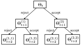
Figure 5: The possible outcomes in two iterations of a Metropolis-Hastings sampler.

Prefetching: The idea of prefetching is to make use of parallel processing to calculate multiple likelihoods ahead of time, and only use the ones which are needed. Consider a generic random-walk metropolis-Hastings algorithm at time $t$. The subsequent steps can be represented by a binary tree, where at each iteration a single new proposal is drawn from a proposal distribution and stochastically accepted or rejected. So, at time $t+n$ the chain has $2^{n}$ possible future states, as illustrated in Fig. 5. The vanilla version of prefetching speculatively evaluates all paths in this binary tree [41]. Since only one path of these will be taken, with $M$ cores, this approach achieves a speedup of $\log_{2}M$ with respect to single core execution, ignoring communication overheads. More efficient prefetching approaches have been proposed in [17] and [167] by better guessing the probabilities of exploration of both the acceptance and the rejection branches at each node. The recent work [20] presents a delayed acceptance strategy for MH testing, which can be used to improve the efficiency of prefetching.

As a special type of MCMC, Gibbs sampling methods naturally follow a blocking scheme by iterating over some partition of the variables. The early asynchronous Gibbs sampler [68] is highly parallel by sampling all variables simultaneously on separate processors. However, the extreme parallelism comes at a cost, e.g., the sampler may not converge to the correct stationary distribution in some cases [76]. The work [76] develops various variable partitioning strategies to achieve fast parallelization, while maintaining the convergence to the target posterior, and the work [92] analyzes the convergence and correctness of the asynchronous Gibbs sampler (a.k.a, the Hogwild parallel Gibbs sampler) for sampling from Gaussian distributions. Many other parallel Gibbs sampling algorithms have been developed for specific models. For example, various distributed Gibbs samplers [138, 164, 9, 117, 46] have been developed for the vanilla LDA, [47] develops a distributed Gibbs sampler via data augmentation to learn large-scale topic graphs with a logistic-normal topic model, and parallel algorithms for DP mixtures have been developed by introducing auxiliary variables for additional CI structures [189], while with the potential risk of causing extremely imbalanced partitions [65].

Note that the stochastic methods and distributed computing are not exclusive. Combing both often leads to more efficient solutions. For example, for optimization methods, parallel SGD methods have been extensively studied [206, 139]. In particular, [139] presents a parallel SGD algorithm without locks, called Hogwild!, where multiple processors are allowed equal access to the shared memory and are able to update individual components of memory at will. Such a scheme is particularly suitable for sparse learning problems. For Bayesian methods, the distributed stochastic gradient Langevin dynamics (D-SGLD) method has been developed in [11] and further improved for topic models in [194].

5 Tools, Software and Systems

Though stochastic algorithms are easy to implement, distributed methods often need a careful design of the system architectures and programming libraries. For system architectures, we may have a shared memory computer with many cores, a cluster with many machines interconnected by network (either commodity or high-speed), or accelerating hardware like graphics processing units (GPUs) and field-programmable gate arrays (FPGAs). We now review the distributed programming frameworks suitable for various system architectures and existing tools for Bayesian inference.

5.1 System Primitives

Every architecture has its low-level libraries, in which the parallel computing units (e.g., threads, machines, or GPU cores) are explicitly visible to the programmer.

Shared Memory Computer: A shared memory computer passes data from one CPU core to another by simply storing it into the main memory. Therefore, the communication latency is low. It is also easy to program and acquire. Meanwhile it is prevalent—it is the basic component of large distributed clusters and host of GPUs or other accelerating hardware. Due to these reasons, writing a multi-thread program is usually the first step towards large-scale learning. However, its drawbacks include limited memory/IO capacity and bandwidth, and restricted scalability, which can be addressed by distributed clusters.

Programmers work with threads in a shared memory setting. A threading library supports: 1) spawning a thread and wait it to complete; 2) synchronization: method to prevent conflict access of resources, such as locks; 3) atomic: operations, such as increment that can be executed in parallel safely. Besides threads and locks, there are alternative programming frameworks. For example, Scala uses actor, which responds to a message that it receives; Go uses channel, which is a multi-provider, multi-consumer queue. There are also libraries automating specific parallel pattern, e.g., OpenMP [6] supports parallel patterns like parralel for or reduction, and synchronization patterns like barrier; TBB [4] has pipeline, lightweight green threads and concurrent data structures. Choosing right programming models sometimes can simplify the implementation.

Accelerating Hardware: GPUs are self-contained parallel computational devices that can be housed in desktop or laptop computers. A single GPU can provide floating operations per second (FLOPS) performance as good as a small cluster. Yet compared to conventional multi-core processors, GPUs are cheap, easily accessible, easy to maintain, easy to code, and dedicated local devices with low power consumption. GPUs follow a single instruction multiple data (SIMD) pattern, i.e., a single program will be executed on all cores given different data. This pattern is suitable for many ML applications. However, GPUs may be limited due to: 1) small memory capacity; 2) restricted SIMD programming model; and 3) high CPU-GPU or GPU-GPU communication latency.

Many Bayesian inference methods have been accelerated with GPUs. For example, [168] adopts GPUs to parallelize the likelihood evaluation in MCMC; [110] provides GPU parallelization for population-based MCMC methods [88] as well as SMC samplers [132]; and [25] uses GPU computing to develop fast Hamiltonian Monte Carlo methods. For variational Bayesian methods, [193] demonstrates an example of using GPUs to accelerate the collapsed variational Bayesian algorithm for LDA. More recently, SaberLDA [114] implements a sparsity-aware sampling algorithm on GPU, which scales sub-linearly with the number of topics. BIDMach [44] is a distributed GPU framework for machine learning, In particular, BIDMach LDA with a single GPU is able to learn faster than the state-of-the-art CPU based LDA implementation [9], which use 100 CPUs.

Finally, acceleration with other hardware (e.g., FPGAs) has also been investigated [45].

Distributed Cluster: For distributed clusters, a low-level framework should allow users to do: 1) Communication: sending and receiving data from/to another machine or a group of machines; 2) Synchronization: synchronize the processes; 3) Fault handling: decide what to do if a process/machine breaks down. For example, MPI provides a set of primitives including send, receive, broadcast and reduce for communication. MPI also provides synchronization operations, such as barrier. MPI handles fault by simply terminating all processes. MPI works on various network infrastructures, such as ethernet or Infiniband. Besides MPI, there are other frameworks that support communication, synchronization and fault handling, such as 1) message queues, where processes can put and get messages from globally shared message queues; 2) remote procedural calls (RPCs), where a process can invoke a procedure in another process, passing its own data to that remote procedure, and finally get execution results. MrBayes [156, 13] provides a MPI-based parallel algorithm for Metropolis-coupled MCMC for Bayesian phylogenetic inference.

Programming with system primitive libraries are most flexible and lightweight. However for sophisticated applications, which may require asynchronous execution, need to modify the global parameters while running, or need many parallel execution blocks, it would be painful and error prone to write the parallel code using the low-level system primitives. Below, we review some high-level distributed computing frameworks, which automatically execute the user declared tasks on desired architectures. We refer the readers to [27] for more details on GPUs, MapReduce, and some other examples (e.g., parallel online learning).

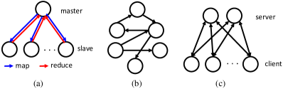
Figure 6: Various architectures: (a) MapReduce/Spark; (b) Pregel/GraphLab; (c) Parameter servers.

5.2 MapReduce and Spark

MapReduce [54] is a distributed computing framework for key-value stores. It reads key-value stores from disk, performs some transformations to these key-value stores in parallel, and writes the final results to disk. A typical MapReduce cycle involves the steps: (1) Spawn some workers on all machines; (2) Workers read input key-value pairs in parallel from a distributed file system; (3) Map: Pass each key-value pair to a user defined function, which will generate some intermediate key-value pairs; (4) According to the key, hash the intermediate key-value pairs to all machines, then merge key-value pairs that have the same key, result with (key, list of values) pairs; (5) Reduce: In parallel, pass each (key, list of values) pairs to a user defined function, which will generate some output key-value pairs; and (6) Write output key-value pairs to the file system.

There are two user defined functions, mapper and reducer. For ML, a key-value store is often data samples, mapper is often used for computing latent variables, likelihoods or gradients for each data sample, and reducer is often used to aggregate the information from each data sample, where the information can be used for estimating parameters or checking convergence. [49] discusses a number of ML algorithms on MapReduce, including linear regression, naive Bayes, neural networks, PCA, SVM, etc. Mahout [1] is a ML package built upon Hadoop, an open source implementation of MapReduce. Mahout provides collaborative filtering, classification, clustering, dimensionality reduction and topic modeling algorithms. [197] is a MapReduce based LDA. However, a major drawback of MapReduce is that it needs to read the data from disk at every iteration. The overhead of reading data becomes dominant for many iterative ML algorithms as well as interactive data analysis tools [196].

Spark [196] is another framework for distributed ML methods that involve iterative jobs. The core of Spark is resilient data sets (RDDs), which is essentially a dataset distributed across machines. RDD can be stored either in memory or disk: Spark decides it automatically, and users can provide hints to Spark which to store in memory. This avoids reading the dataset at every iteration. Users can perform parallel operations to RDDs, which will transform a RDD to another. Available parallel operations are like foreach and reduce. We can use foreach to do the computation for each data, and use reduce to aggregate information from data. Because parallel operations are just a parallel version of the corresponding serial operations, a Spark program looks almost identical to its serial counterpart. Spark can outperform Hadoop for iterative ML jobs by 10x, and is able to interactively query a 39GB dataset in 1 second [196].

5.3 Iterative Graph Computing

Both MapReduce and Spark have a star architecture as in Fig. 6 (a), where only master-slave communication is permitted; they do not allow one key-value pair to interact with another, e.g., reading or modifying the value of another key-value pair. The interaction is necessary for applications like PageRank, Gibbs sampling, and variational Bayes optimized by coordinate descent, all of which require variables to get their own values based on other related variables. Hence there comes graph computing, where the computational task is defined by a sparse graph that specifies the data dependency, as shown in Fig. 6 (b).

Pregel [122] is a bulk synchronous parallel (BSP) graph computing engine. The computation model is a sparse graph with data on vertices and edges, where each vertex receives all messages sent to it in the last iteration; updates data on the vertex based on the messages; and sends out messages along adjacent edges. For example, Gibbs sampling can be done easily by sending the vertex statistics to adjacent vertices and then the conditional probability can be computed. GPS [158] is an open source implementation of Pregel with new features (e.g., dynamic graph repartition).

GraphLab [119] is a more sophisticated graph computing engine that allows asynchronous execution and flexible scheduling. A GraphLab iteration picks up a vertex $v$ in the task queue; and passes the vertex to a user defined function, which may modify the data on the vertex, its adjacent edges and vertices, and finally may add its adjacent vertices to the task queue. Note that several nodes can be evaluated in parallel as long as they do not violate the consistency guarantee which ensures that GraphLab is equivalent with some serial algorithm. It has been used to parallelize a number of ML tasks, including matrix factorization, Gibbs sampling and Lasso [119]. [204] presents a distributed Gibbs sampler on GraphLab for an improved sLDA model using RegBayes. Several other graph computing engines have been developed. For example, GraphX [191] is an extension of Spark for graph computing; and GraphChi [104] is a disk based version of GraphLab.

5.4 Parameter Servers

All the above frameworks restrict the communication between workers. For example, MapReduce and Spark don’t allow communication between workers, while Pregel and GraphLab only allow vertices to communicate with adjacent nodes. On the other side, many ML methods follow a pattern that: (1) Data are partitioned on many workers; (2) There are some shared global parameters (e.g., the model weights in a gradient descent method or the topic-word count matrix in the collapsed Gibbs sampler for LDA [80]); and (3) Workers fetch data and update (parts of) global parameters based on their local data (e.g., using the local gradients or local sufficient statistics). Though it is straightforward to implement on shared memory computers, it is rather difficult in a distributed setting. The goal of parameter servers is to provide a distributed data structure for parameters.

A parameter server is a key-value store (like a hash map), accessible for all workers. It supports for get and set (or update) for each entry. In a distributed setting, both server and client consist of many nodes (see Fig. 6 (c)). Memcached [3] is an in memory key-value store that provides get and set for arbitrary data. However it doesn’t have a mechanism to resolve conflicts raised by concurrent access, e.g. concurrent writes for a single entry. Applications like [164] require to lock the global entry while updating, which leads to suboptimal performance. Piccolo [147] addresses this by introducing user-defined accumulations, which correctly address concurrent updates to the same key. Piccolo has a set of built-in user defined accumulations such as summation, multiplication, and min/max.

One important tradeoff made by parameter servers is that they sacrifice consistency for less latency—get may not return the most recent value, so that it can return immediately without waiting for most recent updates to reach the server. While this improves the performance significantly, it can potentially slow down convergence due to outdated parameters. [85] proposed Stale Synchronous Parallel (SSP), where the staleness of parameters is bounded and the fastest worker can be ahead of the slowest one by no more than $\tau$ iterations, where $\tau$ can be tuned to get a fast convergence as well as low waiting time. Petuum [51] is a SSP based parameter server. [115] proposed communication-reducing improvements, including key caching, message compression and message filtering, and it also supports elastically adding and removing both server and worker nodes.

Parameter servers have been deployed in learning very large-scale logistic regression [115], deep networks [53], LDA [9, 112] and Lasso [51]. [115] learns a 2000-topic LDA with 5 billion documents and 5 million unique tokens on 6000 machines in 20 hours. Yahoo! LDA [9] has a parameter server designed specifically for Bayesian latent variable models and it is the fastest available LDA software. There are a bunch of distributed topic modeling softwares based on Yahoo! LDA, including [205] for MedLDA and [47] for correlated topic models.

5.5 Model Parallel Inference

MapReduce, Spark and Parameter servers take the data-parallelism approach, where data are partitioned across machines and computations are performed on each node given a copy of the globally shared model. However, as the model size rapidly grows (i.e., the large $M$ challenge), the models cannot fit in a single computer’s memory. Model-parallelism addresses this challenge by partitioning the model and storing a part of the model on each node. Then, partial updates (i.e., the updates of model parts) are carried out on each node. Benefits of model-parallelism include large model sizes, flexibility to focus workers on fastest-converging parameters, and more accurate convergence because no delayed update is involved.

STRADS [111] provides primitives for model-parallelism and it handles the distributed storage of model and data automatically. STRADS requires that a partial update could be computed using just the model part together with data. Users writes schedule that assigns model sets to workers, push that computes the partial updates for model, pop that applies updates to model. An automatic sync primitive will ensure that users always get the latest model. As a concrete example, [199] demonstrates a model parallel LDA, in which both data and model are partitioned by vocabulary. In each iteration, a worker only samples latent variables and updates the model related to the vocabulary part assigned to it. The model then rotates between workers, until a full cycle is completed. Unlike data parallel LDA [164, 9, 138], the sampler always uses the latest models and no read-write lock is needed on models, thereby leading to faster convergence than data-parallel LDAs.

Note that model-parallelism is not a replacement but a complement of data-parallelism. For example, [182] showed a two layer LDA system, where layer 1 is model-parallelism and layer 2 consists of several local model-parallelism clusters performing asynchronous updates on an globally distributed model.

6 Conclusions and Perspectives

We present a survey of recent advances on big learning with Bayesian methods, including Bayesian nonparametrics, regularized Bayesian inference, and scalable inference algorithms and the systems based-on stochastic subsampling or distributed computing. It is helpful to note that our review is not exhaustive. In fact, big learning has attracted intense interest with active research spanning diverse fields, including machine learning, databases, parallel and distributed systems, and programming languages.

As reviewed above, big learning with Bayesian methods has achieved substantial progress. However, considerable challenges still remain. We briefly discuss several directions that are of promise for future investigation. First, Bayesian methods have the advantage to incorporate prior knowledge for efficient learning, especially for the scenarios where a large number of training data is lacking, and characterize uncertainty. For instance, the recent work [105] demonstrates an example for the challenging task of one-shot learning, which achieves human-level performance by encoding the domain knowledge as a hierarchical Bayesian model. In contrast, deep learning methods [109] stand at the other end of the spectrum—they are often learned in an end-to-end manner by feeding a large set of training data, and they often do not represent the uncertainty in the structure or parameters of the neural networks. A natural and important question that remains under-addressed is how to conjoin the flexibility of deep learning and the learning efficiency of Bayesian methods for robust learning. Another related important question is how to effectively collect domain knowledge and incorporate it into the modeling and inference process. The work [126] has demonstrated an example that selectively incorporates the noisy knowledge collected from crowds for robust Bayesian inference, but much more are left unexplored.

Second, one of the lessons we learn from big learning is that the best predictive performance is often obtained by building a highly flexible model (e.g., deep neural networks [109]). Although nonparametric Bayesian techniques are powerful in theory to represent flexible models and automatically infer their complexity from an unbounded space, there is still a large gap in practice, with very few real applications. Most of the evaluations are proof-of-concepts by being hindered on small-scale problems or those with relatively simple structures. For example, although some attempts have demonstrated that a cascade IBP can be applied to infer the structure of a sparse deep belief network [8], these results are preliminary and can only learn toy network structures. It needs further study on how to learn the structure of a sophisticated network with state-of-the-art performance. In order to fill up the practical gap of nonparametric models, we need to develop the algorithms that are accurate and scalable as well as the theory of defining flexible nonparametric processes that can properly consider the rich structures in various domains.

Third, a more powerful way of composing Bayesian models is offered by probabilistic programming, which uses general-purpose computer programs to represent probabilistic models and automates the inference procedure by building a universal engine. Several probabilistic programming languages have been developed, including BUGS, Stan, BLOG, Church and Infer.Net. However, scalable inference is still a considerable challenge for these languages. The existing platforms for Bayesian inference do not well support the advanced deep models and the recent scalable algorithms in distributed/stochastic settings. They do not well support the accelerating hardware (e.g., GPUs and FPGAs) either. In fact, the existence of user-friendly platforms (e.g., Tensorflow [7], Theano [174] and Caffe [91]) has significantly boosted the applications of deep learning in industry. It will be very useful to fill up this gap for Bayesian methods, which can allow for rapid prototyping and testing of different models, therefore motivating wider adoption of Bayesian methods. Edward is a recent system that builds on Tensorflow for scalable Bayesian inference, but much work needs to be done.

Finally, the current machine learning methods in general still require considerable human expertise in devising appropriate features, priors, models, and algorithms. Much work has to be done in order to make ML more widely used and eventually become a common part of our day to day tools in data sciences. Along this line, several promising projects have been started. Google prediction API is one of the earliest efforts that try to make ML accessible for beginners by providing easy-to-use service. Microsoft AzureML takes a similar approach by providing a visual interface to help design experiments. SystemML [75] provides an R-like declarative language to specify ML tasks based on MapReduce, and MLBase [103] further improves it by providing learning-specific optimizer that transforms a declarative task into a sophisticated learning plan. Finally, Automated Statistician (AutoStat) [118] aims to automate the process of statistical modeling, by using Bayesian model selection strategies to automatically choose good models/features and to interpret the results in easy-to-understand ways, in terms of automatically generated reports. Though still at a very early stage, such efforts would have a tremendous impact on the fields that currently rely on expert statisticians, ML researchers, and data scientists.

References

- [1] Apache mahout: https://mahout.apache.org/.
- [2] http://lshtc.iit.demokritos.gr/.
- [3] http://memcached.org.
- [4] https://www.threadingbuildingblocks.org/.
- [5] http://www.image-net.org/about-overview.
- [6] http://www.openmp.org.
- [7] M. Abadi, A. Agarwal, P. Barham, E. Brevdo, Z. Chen, C. Citro, G. S. Corrado, A. Davis, J. Dean, M. Devin, S. Ghemawat, I. Goodfellow, A. Harp, G. Irving, M. Isard, Y. Jia, R. Jozefowicz, L. Kaiser, M. Kudlur, J. Levenberg, D. Mané, R. Monga, S. Moore, D. Murray, C. Olah, M. Schuster, J. Shlens, B. Steiner, I. Sutskever, K. Talwar, P. Tucker, V. Vanhoucke, V. Vasudevan, F. Viégas, O. Vinyals, P. Warden, M. Wattenberg, M. Wicke, Y. Yu, and X. Zheng. TensorFlow: Large-scale machine learning on heterogeneous systems, 2015. Software available from tensorflow.org.
- [8] R. Adams, H. Wallach, and Z. Ghahramani. Learning the structure of deep sparse graphical models. In AISTATS, 2010.
- [9] A. Ahmed, M. Aly, J. Gonzalez, S. Narayanamurthy, and A. Smola. Scalable inference in latent variable models. In WSDM, 2012.
- [10] S. Ahn, A. Korattikara, and M. Welling. Bayesian posterior sampling via stochastic gradient fisher scoring. In ICML, 2012.
- [11] S. Ahn, B. Shahbaba, and M. Welling. Distributed stochastic gradient MCMC. In ICML, 2014.
- [12] J. Aitchison and S. M. Shen. Logistic-normal distributions: Some properties and uses. Biometrika, 67(2):261–272, 1980.
- [13] G. Altekar, S. Dwarkadas, J. Huelsenbeck, and F. Ronquist. Parallel Metropolis coupled Markov chain Monte Carlo for Bayesian phylogenetic inference. Bioinformatics, 20(3):407–415, 2004.
- [14] S. Amari. Natural gradient works efficiently in learning. Neural Comput., 10:251–276, 1998.
- [15] C. Andrieu, A. Doucet, and R. Holenstein. Particle Markov chain Monte Carlo methods. J. R. Stat. Soc., Ser B, 72(3):269–342, 2010.
- [16] C. Andrieu, N. D. Freitas, A. Doucet, and M. I. Jordan. An introduction to MCMC for machine learning. Machine Learning, 50:5–43, 2003.
- [17] E. Angelino, E. Kohler, A. Waterland, M. Seltzer, and R. P. Adams. Accelerating MCMC via parallel predictive prefetching. arXiv:1403.7265, 2014.
- [18] C. Antoniak. Mixture of Dirichlet process with applications to Bayesian nonparametric problems. Ann. Stats., (273):1152–1174, 1974.
- [19] M. Arulampalam, S. Maskell, N. Gordon, and T. Clapp. A tutorial on particle filters for online nonlinear/non-gaussian Bayesian tracking. IEEE Trans. Signal Process., 50(2):174–188, 2002.
- [20] M. Banterle, C. Grazian, and C. P. Robert. Accelerating Metropolis-Hastings algorithms: Delayed acceptance with prefetching. arXiv:1406.2660, 2014.
- [21] R. Bardenet, A. Doucet, and C. Holmes. Towards scaling up Markov chain Monte Carlo: an adaptive subsampling approach. In ICML, 2014.
- [22] R. Bardenet and O.-A. Maillard. Concentration inequalities for sampling without replacement. arXiv:1309.4029, 2013.
- [23] M. Beal, Z. Ghahramani, and C. Rasmussen. The infinite hidden markov model. In NIPS, 2002.
- [24] M. J. Beal. Variational algorithms for approximate Bayesian inference. PhD Thesis, University of Cambridge, 2003.
- [25] A. L. Beam, S. K. Ghosh, and J. Doyle. Fast Hamiltonian Monte Carlo using GPU computing. arXiv:1402.4089, 2014.
- [26] A. Beck and S. Sabach. Weiszfeld s method: Old and new results. J. of Opt. Theory and Applications, 2014.
- [27] R. Bekkerman, M. Bilenko, and J. Langford. Scaling up machine learning: Parallel and distributed approaches. Cambridge University Press, 2011.
- [28] S. Bengio, J. Weston, and D. Grangier. Label embedding trees for large multi-class tasks. In NIPS, 2010.
- [29] Y. Bengio, A. Courville, and P. Vincent. Representation Learning: A Review and New Perspectives. IEEE Trans. on PAMI, 35(8):1798–1828, 2013.
- [30] W. Bialek, I. Nemenman, and N. Tishby. Predictability, complexity and learning. Neural Comput., 13:2409–2463, 2001.
- [31] C. M. Bishop. Pattern Recognition and Machine Learning. Springer, 2006.
- [32] D. Blei and P. Frazier. Distance dependent Chinese restaurant processes. In ICML, 2010.
- [33] D. Blei and M. Jordan. Variational inference for dirichlet process mixtures. Bayesian Analysis, 1:121–144, 2006.
- [34] D. Blei and J. Lafferty. Correlated topic models. In NIPS, 2006.
- [35] D. Blei and J. McAuliffe. Supervised topic models. In NIPS, 2007.
- [36] D. Blei, A. Ng, and M. I. Jordan. Latent Dirichlet Allocation. JMLR, (3):993–1022, 2003.
- [37] L. Bottou. Online Algorithms and Stochastic Approximations. Online Learning and Neural Networks, Edited by David Saad, Cambridge University Press, Cambridge, UK, 1998.
- [38] L. Bottou and O. Bousquet. The tradeoffs of large scale learning. In NIPS, 2008.
- [39] S. Boyd, N. Parikh, E. Chu, B. Peleato, and J. Eckstein. Distributed Optimization and Statistical Learning via the Alternating Direction Method of Multipliers, volume 3. Foundations and Trends in Machine Learning, 2011.
- [40] S. Boyd and L. Vandenberghe. Convex Optimization. Cambridge University Press, 2004.
- [41] A. Brockwell. Parallel Markov chain Monte Carlo simulation by pre-fetching. JCGS, 15(1):246–261, 2006.
- [42] T. Broderick, N. Boyd, A. Wibisono, A. C. Wilson, and M. I. Jordan. Streaming variational Bayes. In NIPS, 2013.
- [43] G. Brumfiel. High-energy physics: Down the petabyte highway. Nature, 469:282–283, 2011.
- [44] J. Canny and H. Zhao. Bidmach: Large-scale learning with zero memory allocation. In NIPS Big Learning Workshop, 2013.
- [45] T. Chau, J. Targett, M. Wijeyasinghe, W. Luk, P. Cheung, B. Cope, A. Eele, and J. Maciejowski. Accelerating sequential Monte Carlo method for real-time air traffic management. SIGARCH Computer Architecture News, 41(5):35–40, 2013.
- [46] J. Chen, K. Li, J. Zhu, and W. Chen. Warplda: a cache efficient o (1) algorithm for latent dirichlet allocation. In VLDB, 2016.
- [47] J. Chen, J. Zhu, Z. Wang, X. Zheng, and B. Zhang. Scalable inference for logistic-normal topic models. In NIPS, 2013.
- [48] T. Chen, E. B. Fox, and C. Guestrin. Stochastic gradient Hamiltonian Monte Carlo. In ICML, 2014.
- [49] C. Chu, S. K. Kim, Y.-A. Lin, Y. Yu, G. Bradski, A. Y. Ng, and K. Olukotun. Map-reduce for machine learning on multicore. In NIPS, 2007.
- [50] K. Crammer, O. Dekel, J. Keshet, S. Shalev-Shwartz, and Y. Singer. Online passive-agressive algorithms. JMLR, (7):551–585, 2006.
- [51] W. Dai, J. Wei, X. Zheng, J. K. Kim, S. Lee, J. Yin, Q. Ho, and E. Xing. Petuum: A framework for iterative-convergent distributed ML. In arXiv:1312.7651, 2013.
- [52] P. Dallaire, P. Giguere, and B. Chaib-draa. Learning the structure of probabilistic graphical models with an extended cascading Indian buffet process. In AAAI, 2014.
- [53] J. Dean, G. Corrado, R. Monga, K. Chen, M. Devin, M. Mao, A. Senior, P. Tucker, K. Yang, Q. V. Le, et al. Large scale distributed deep networks. In NIPS, 2012.
- [54] J. Dean and S. Ghemawat. MapReduce: Simplified data processing on large clusters. In OSDI, 2004.
- [55] J. Deng, S. Satheesh, A. Berg, and L. Fei-Fei. Fast and balanced: Efficient label tree learning for large scale object recognition. In NIPS, 2011.
- [56] C. Doctorow. Big data: Welcome to the petacentre. Nature, 455:16–21, 2008.
- [57] S. Donnet, V. Rivoirard, J. Rousseau, and C. Scricciolo. On convergence rates of empirical Bayes procedures. In 47th Scientific Meeting of the Italian Statistical Society, 2014.
- [58] F. Doshi-Velez, K. Miller, J. V. Gael, and Y. W. Teh. Variational inference for the Indian buffet process. In AISTATS, 2009.
- [59] J. Duan, M. Guindani, and A. Gelfand. Generalized spatial Dirichlet process models. Biometrika, 94(4), 2007.
- [60] J. Duchi, E. Hazan, and Y. Singer. Adaptive subgradient methods for online learning and stochastic optimization. JMLR, 12:2121–2159, 2011.
- [61] D. V. Dyk and X. Meng. The art of data augmentation. JCGS, 10(1):1–50, 2001.
- [62] B. Efron. Bayes’ theorem in the 21st century. Science, 340(6137):1177–1178, 2013.
- [63] J. Fan, F. Han, and H. Liu. Challenges of big data analysis. National Science Review, 1(2):293–314, 2013.
- [64] T. Ferguson. A Bayesian analysis of some nonparametric problems. Ann. Stats., (1):209–230, 1973.
- [65] Y. Gal and Z. Ghahramani. Pitfalls in the use of parallel inference for the Dirichlet process. In ICML, 2014.
- [66] A. Gelman, J. Carlin, H. Stern, D. Dunson, A. Vehtari, and D. Rubin. Bayesian Data Analysis. Third Edition, Chapman & Hall/CRC Texts in Statistical Science), 2013.
- [67] A. Gelman and D. Rubin. Inference from iterative simulation using multiple simulations. Statist. Sci., 7(4):457–511, 1992.
- [68] S. Geman and D. Geman. Stochastic relaxation, Gibbs distributions, and the Bayesian restoration of images. IEEE Trans. on PAMI, 6(1):721–741, 1984.
- [69] E. I. George and D. P. Foster. Calibration and empirical Bayes variable selection. Biometrika, 87(4):731–747, 2000.
- [70] S. Gershman, P. Frazier, and D. Blei. Distance dependent infinite latent feature models. arXiv:1110.5454, 2011.
- [71] S. Gershmana and D. Blei. A tutorial on Bayesian nonparametric models. J. Math. Psychol., (56):1–12, 2012.
- [72] C. J. Geyer and E. A. Thompson. Annealing Markov chain Monte Carlo with applications to ancestral inference. JASA, 90(431):909–920, 1995.
- [73] Z. Ghahramani. Bayesian nonparametrics and the probabilistic approach to modelling. Phil. Trans. of the Royal Society, 2013.
- [74] J. K. Ghosh and R. Ramamoorthi. Bayesian Nonparametrics. Springer, New York, NY, 2003.
- [75] A. Ghoting, R. Krishnamurthy, E. Pednault, B. Reinwald, V. Sindhwani, and et al. SystemML: Declarative machine learning on MapReduce. In ICDE, 2011.
- [76] J. E. Gonzalez, Y. Low, A. Gretton, and C. Guestrin. Parallel Gibbs sampling: From colored fields to thin junction trees. In AISTATS, 2011.
- [77] P. Gopalan and D. Blei. Efficient discovery of overlapping communities in massive networks. PNAS, 110(36):14534–14539, 2013.
- [78] A. Grelaud, C. P. Robert, J.-M. Marin, F. Rodolphe, and J.-F. Taly. Likelihood-free methods for model choice in Gibbs random fields. Bayesian Analysis, 4(2):317–336, 2009.
- [79] T. Griffiths and Z. Ghahramani. Infinite latent feature models and the Indian buffet process. In NIPS, 2006.
- [80] T. Griffiths and M. Steyvers. Finding scientific topics. PNAS, 2004.
- [81] R. Guhaniyogi, S. Qamar, and D. Dunson. Bayesian conditional density filtering for big data. arXiv:1401.3632, 2014.
- [82] W. Hastings. Monte Carlo sampling methods using Markov chains and their applications. Biometrika, 57(1):97–109, 1970.
- [83] G. Hinton, L. Deng, D. Yu, A. Mohamed, N. Jaitly, and etc. Deep neural networks for acoustic modeling in speech recognition. IEEE Signal Process. Mag., 29(6):82–97, 2012.
- [84] N. Hjort, C. Holmes, P. Muller, and S. Walker. Bayesian Nonparametrics: Principles and Practice. Cambridge University Press, 2010.
- [85] Q. Ho, J. Cipar, H. Cui, S. Lee, J. Kim, P. Gibbons, G. Gibson, G. Ganger, and E. Xing. More effective distributed ML via a stale synchronous parallel parameter server. In NIPS, 2013.
- [86] M. D. Hoffman, D. Blei, C. Wang, and J. Paisley. Stochastic variational inference. JMLR, 14:1303–1347, 2013.
- [87] T. Hofmann, B. Scholkopf, and A. J. Smola. Kernel methods in machine learning. Ann. Statist., 36(3):1171–1220, 2008.
- [88] A. Jasra, D. A. Stephens, and C. C. Holmes. On population-based simulation for static inference. Statistics and Computing, 17(3):263–279, 2007.
- [89] E. T. Jaynes. Prior probabilities. IEEE Trans. on Sys. Sci. and Cybernetics, 4:227–241, 1968.
- [90] H. Jeffreys. An invariant form for the prior probability in estimation problems. Proc. of the Royal Society of London. Series A, Mathematical and Physical Sciences, 186(1007):453–461, 1945.
- [91] Y. Jia, E. Shelhamer, J. Donahue, S. Karayev, J. Long, R. Girshick, S. Guadarrama, and T. Darrell. Caffe: Convolutional architecture for fast feature embedding. arXiv preprint arXiv:1408.5093, 2014.
- [92] M. J. Johnson, J. Saunderson, and A. S. Willsky. Analyzing hogwild parallel gaussian Gibbs sampling. In NIPS, 2013.
- [93] M. Jordan. The era of big data. ISBA Bulletin, 18(2):1–3, 2011.
- [94] M. Jordan, Z. Ghahramani, T. Jaakkola, and L. Saul. An introduction to variational methods for graphical models. MLJ, 37(2):183–233, 1999.
- [95] J. B. Kadane and N. A. Lazar. Methods and criteria for model selection. JASA, 99(465):279–290, 2004.
- [96] R. E. Kalman. A new approach to linear filtering and prediction problems. J. Fluids Eng., 82(1):35–45, 1960.
- [97] R. E. Kass and A. E. Raftery. Bayes factors. JASA, 90(430):773–795, 1995.
- [98] D. I. Kim, P. Gopalan, D. M. Blei, and E. B. Sudderth. Efficient online inference for Bayesian nonparametric relational models. In NIPS, 2013.
- [99] D. Kingma and M. Welling. Auto-encoding variational bayes. In ICLR, 2014.
- [100] D. Kingma and M. Welling. Efficient gradient-based inference through transformations between Bayes nets and neural nets. In ICML, 2014.
- [101] A. Korattikara, Y. Chen, and M. Welling. Austerity in MCMC land: Cutting the Metropolis-Hastings budget. In ICML, 2014.
- [102] O. Koyejo and J. Ghosh. Constrained Bayesian inference for low rank multitask learning. In UAI, 2013.
- [103] T. Kraska, A. Talwalkar, J. Duchi, R. Griffith, M. Franklin, and M. Jordan. MLbase: A distributed machine-learning system. In CIDR, 2013.
- [104] A. Kyrola, G. E. Blelloch, and C. Guestrin. GraphChi: Large-scale graph computation on just a PC. In OSDI, 2012.
- [105] B. Lake, R. Salakhutdinov, and J. Tenenbaum. Human-level concept learning through probabilistic program induction. Science, 350(6266):1332–1338, 2015.
- [106] S. L. Lauritzen. Propagation of probabilities, means and variances in mixed graphical association models. JASA, 87:1098–1108, 1992.
- [107] N. Lawrence. Probabilistic non-linear principal component analysis with Gaussian process latent variable models. JMLR, (6):1783–1816, 2005.
- [108] Q. Le, M. Ranzato, R. Monga, M. Devin, K. Chen, G. Corrado, J. Dean, and A. Ng. Building high-level features using large scale unsupervised learning. In ICML, 2012.
- [109] Y. LeCun, Y. Bengio, and G. Hinton. Deep learning. Nature, 521:436–444, 2015.
- [110] A. Lee, C. Yau, M. B. Giles, A. Doucet, and C. C. Holmes. On the utility of graphics cards to perform massively parallel simulation of advanced Monte Carlo methods. JCGS, 19(4):769–789, 2010.
- [111] S. Lee, J. K. Kim, X. Zheng, Q. Ho, G. Gibson, and E. Xing. Primitives for dynamic big model parallelism. arXiv:1406.4580, 2014.
- [112] A. Q. Li, A. Ahmed, S. Ravi, and A. J. Smola. Reducing the sampling complexity of topic models. In SIGKDD, 2014.
- [113] F.-F. Li and P. Perona. A bayesian hierarchical model for learning natural scene categories. In CVPR, 2005.
- [114] K. Li, J. Chen, W. Chen, and J. Zhu. Saberlda: Sparsity-aware learning of topic models on gpus. arXiv preprint arXiv:1610.02496, 2016.
- [115] M. Li, D. Andersen, J. W. Park, A. Smola, A. Ahmed, V. Josifovski, J. Long, E. Shekita, and B.-Y. Su. Scaling distributed machine learning with the parameter server. In OSDI, 2014.
- [116] J. S. Liu and R. Chen. Sequential Monte Carlo methods for dynamic systems. JASA, 93(443):1032–1044, 1998.
- [117] Z. Liu, Y. Zhang, E. Y. Chang, and M. Sun. PLDA+: Parallel latent Dirichlet allocation with data placement and pipeline processing. TIST, 2(3), 2011.
- [118] J. Lloyd, D. Duvenaud, R. Grosse, J. Tenenbaum, and Z. Ghahramani. Automatic construction and natural language description of nonparametric regression models. In AAAI, 2014.
- [119] Y. Low, J. Gonzalez, A. Kyrola, D. Bickson, C. Guestrin, and J. Hellerstein. Graphlab: A new framework for parallel machine learning. In UAI, 2013.
- [120] S. MacEachern. Dependent nonparametric processes. In ASA proceedings of the section on Bayesian statistical science, 1999.
- [121] D. Maclaurin and R. P. Adams. Firefly Monte Carlo: Exact MCMC with subsets of data. In UAI, 2014.
- [122] G. Malewicz, M. H. Austern, A. J. Bik, J. C. Dehnert, I. Horn, N. Leiser, and G. Czajkowski. Pregel: a system for large-scale graph processing. In SIGMOD, 2010.
- [123] S. Mandt and D. Blei. Smoothed gradients for stochastic variational inference. arXiv:1406.3650, 2014.
- [124] B. Marlin, E. Khan, and K. Murphy. Piecewise bounds for estimating Bernoulli-logistic latent Gaussian models. In ICML, 2011.
- [125] J. D. McAuliffe, D. M. Blei, and M. I. Jordan. Nonparametric empirical Bayes for the Dirichlet process mixture model. Statistics and Computing, 16(1):5–14, 2006.
- [126] S. Mei, J. Zhu, and X. Zhu. Robust RegBayes: Selectively incorporating first-order logic domain knowledge into Bayesian models. In ICML, 2014.
- [127] N. Metropolis, A. Rosenbluth, M. Rosenbluth, A. Teller, and E. Teller. Equation of state calculations by fast computing machines. J. Chem. Phys, 21(6):1087, 1953.
- [128] K. Miller, T. Griffiths, and M. Jordan. Nonparametric latent feature models for link prediction. In NIPS, 2009.
- [129] S. Minsker, S. Srivastava, L. Lin, and D. B. Dunson. Scalable and robust Bayesian inference via the median posterior. In ICML, 2014.
- [130] T. Mitchell. Machine Learning. McGraw Hill, 1997.
- [131] A. Mnih and K. Gregor. Neural variational inference and learning in belief networks. In ICML, 2014.
- [132] P. D. Moral, A. Doucet, and A. Jasra. Sequential Monte Carlo samplers. J. R. Stat. Soc., Ser B, 68(3):411–436, 2006.
- [133] P. Muller and F. A. Quintana. Nonparametric Bayesian data analysis. Statistical Science, 19(1):95–110, 2004.
- [134] R. Neal. Markov chain sampling methods for Dirichlet process mixture models. JCGS, pages 249–265, 2000.
- [135] R. Neal. Slice sampling. Ann. Statist., 31(3):705–767, 2003.
- [136] R. Neal. MCMC using Hamiltonian Dynamics. Handbook of Markov Chain Monte Carlo (S. Brooks, A. Gelman, G. Jones, and X.-L. Meng, eds.), Chapman & Hall / CRC Press, 2010.
- [137] W. Neiswanger, C. Wang, and E. P. Xing. Asymptotically exact, embarrassingly parallel MCMC. In UAI, 2014.
- [138] D. Newman, A. Asuncion, P. Smyth, and M. Welling. Distributed inference for latent Dirichlet allocation. In NIPS, 2007.
- [139] F. Niu, B. Recht, C. Re, and S. J. Wright. Hogwild: A lock-free approach to parallelizing stochastic gradient descent. In NIPS, 2011.
- [140] M. Opper. A Bayesian Approach to Online Learning. Online Learning in Neural Networks, Cambridge University, 1999.
- [141] J. Paisley, D. M. Blei, and M. I. Jordan. Variational Bayesian inference with stochastic search. In ICML, 2012.
- [142] O. Papaspiliopoulos, G. O. Roberts, and M. Skold. A general framework for the parametrization of hierarchical models. Statistical Science, 22(1):59–73, 2007.
- [143] S. Patterson and Y. W. Teh. Stochastic gradient Riemannian Langevin dynamics on the probability simplex. In NIPS, 2013.
- [144] S. Petrone, J. Rousseau, and C. Scricciolo. Bayes and empirical Bayes: do they merge? Biometrika, pages 1–18, 2014.
- [145] N. Pillai and A. Smith. Ergodicity of approximate MCMC chains with applications to large data sets. arXiv:1405.0182, 2014.
- [146] J. Pitman. Combinatorial stochastic processes. Technical Report No. 621. Department of Statistics, UC, Berkeley, 2002.
- [147] R. Power and J. Li. Piccolo: Building fast, distributed programs with partitioned tables. In OSDI, 2010.
- [148] L. R. Rabiner. A tutorial on hidden Markov models and selected applications in speech recognition. Proc. of the IEEE, 77(2):257–286, 1989.
- [149] R. Ranganath, C. Wang, D. Blei, and E. Xing. An adaptive learning rate for stochastic variational inference. In ICML, 2013.
- [150] C. E. Rasmussen and C. K. I. Williams. Gaussian Processes for Machine Learning. The MIT Press, 2006.
- [151] O. Reichman, M. Jones, and M. Schildhauer. Challenges and opportunities of open data in ecology. Science, 331(6018):703–705, 2011.
- [152] D. J. Rezende, S. Mohamed, and D. Wierstra. Stochastic backpropagation and approximate inference in deep generative models. In ICML, 2014.
- [153] C. Robert and G. Casella. Monte Carlo Statistical Methods. Springer, 2005.
- [154] C. P. Robert, J.-M. Cornuet, J.-M. Marin, and N. S. Pillai. Lack of confidence in approximate Bayesian computation model choice. PNAS, 108(37):15112–15117, 2011.
- [155] G. Roberts and O. Strame. Langevin diffusions and Metropolis-Hastings algorithms. Methodology and Computing in Applied Probability, 4:337–357, 2002.
- [156] F. Ronquist and J. Huelsenbeck. MrBayes: Bayesian inference of phylogenetic trees. Bioinformatics, 19(12):1572–1574, 2003.
- [157] R. Salakhutdinov. Learning deep generative models. PhD Thesis, University of Toronto, 2009.
- [158] S. Salihoglu and J. Widom. GPS: A graph processing system. In SSDBM, 2013.
- [159] N. Schraudolph, J. Yu, and S. Gunter. A stochastic Quasi-Newton method for online convex optimization. In AISTATS, 2007.
- [160] S. Scott, A. Blocker, F. Bonassi, H. Chipman, E. George, and R. McCulloch. Bayes and big data: The consensus Monte Carlo algorithm. EFaB Bayes 250 Workshop, 16, 2013.
- [161] S. L. Scott. Bayesian methods for hidden Markov models. JASA, 97(457):337–351, 2002.
- [162] J. Sethuraman. A constructive definition of dirichlet priors. Statistica Sinica, (4):639–650, 1994.
- [163] T. Shi and J. Zhu. Online Bayesian passive-aggressive learning. In ICML, 2014.
- [164] A. Smola and S. Narayanamurthy. An architecture for parallel topic models. VLDB, 2010.
- [165] J. Snoek, H. Larochelle, and R. P. Adams. Practical Bayesian optimization of machine learning algorithms. In NIPS, 2012.
- [166] N. Srivastava, G. Hinton, A. Krizhevsky, I. Sutskever, and R. Salakhutdinov. Dropout: A simple way to prevent neural networks from overfitting. JMLR, 15:1929–1958, 2014.
- [167] I. Strid. Efficient parallelisation of Metropolis-Hastings algorithms using a prefetching approach. Computational Statistics and Data Analysis, 54:2814–2835, 2010.
- [168] M. Suchard, Q. Wang, C. Chan, J. Frelinger, A. Cron, and M. West. Understanding GPU programming for statistical computation: Studies in massively parallel massive mixtures. JCGS, 19(2):419–438, 2010.
- [169] M. Tan, I. Tsang, and L. Wang. Towards ultrahigh dimensional feature selection for big data. JMLR, (15):1371–1429, 2014.
- [170] M. Tanner and W. Wong. The calculation of posterior distributions by data augmentation. JASA, 82(398):528–540, 1987.
- [171] Y. W. Teh, D. Gorur, and Z. Ghahramani. Stick-breaking construction for the Indian buffet process. In AISTATS, 2007.
- [172] Y. W. Teh, M. I. Jordan, M. J. Beal, and D. M. Blei. Hierarchical Dirichlet processes. JASA, 101(476):1566–1581, 2006.
- [173] Y. W. Teh, A. Thiey, and S. Vollmer. Consistency and fluctuations for stochastic gradient Langevin dynamics. arXiv:1409.0578, 2014.
- [174] Theano Development Team. Theano: A Python framework for fast computation of mathematical expressions. arXiv e-prints, abs/1605.02688, May 2016.
- [175] R. Thibaux and M. I. Jordan. Hierarchical Beta processes and the Indian buffet process. In AISTATS, 2007.
- [176] B. M. Turnera and T. V. Zandtb. A tutorial on approximate Bayesian computation. J. Math. Psychol., 56(2):69–85, 2012.
- [177] D. van Dyk and T. Park. Partially collapsed Gibbs samplers: Theory and methods. JASA, 103(482):790–796, 2008.
- [178] P. Vincent, H. Larochelle, Y. Bengio, and P.-A. Manzagol. Extracting and composing robust features with denoising autoencoders. In ICML, 2008.
- [179] M. Wainwright and M. Jordan. Graphical models, exponential families, and variational inference. Foundations and Trends in Machine Learning, 1(1–2):1–305, 2008.
- [180] S. G. Walker. Sampling the Dirichlet mixture model with slices. Commun Stat - Simul and Comput, 36:45–54, 2007.
- [181] X. Wang and D. B. Dunson. Parallelizing MCMC via Weierstrass sampler. arXiv:1312.4605, 2013.
- [182] Y. Wang, X. Zhao, Z. Sun, H. Yan, L. Wang, Z. Jin, L. Wang, Y. Gao, J. Zeng, Q. Yang, et al. Towards topic modeling for big data. arXiv:1405.4402, 2014.
- [183] K. Weinberger, A. Dasgupta, J. Langford, A. Smola, and J. Attenberg. Feature hashing for large scale multitask learning. In ICML, 2009.
- [184] M. Welling. Exploiting the statistics of learning and inference. In NIPS workshop on ”Probabilistic Models for Big Data”, 2013.
- [185] M. Welling and Y. W. Teh. Bayesian learning via stochastic gradient Langevin dynamics. In ICML, 2011.
- [186] D. Wilkinson. Parallel Bayesian computation. Handbook of Parallel Computing and Statistics, Chapter 18, 2004.
- [187] P. M. Williams. Bayesian conditionalisation and the principle of minimum information. The British Journal for the Philosophy of Science, 31(2), 1980.
- [188] S. Williamson, P. Orbanz, and Z. Ghahramani. Dependent Indian buffet processes. In AISTATS, 2010.
- [189] S. A. Williamson, A. Dubey, and E. P. Xing. Parallel Markov chain Monte Carlo for nonparametric mixture models. In ICML, 2013.
- [190] X.-L. Wu, C. Sun, T. Beissinger, G. Rosa, K. Weigel, N. Gatti, and D. Gianola. Parallel Markov chain Monte Carlo - bridging the gap to high-performance Bayesian computation in animal breeding and genetics. Genetics Seletion Evolution, 44(1):29–46, 2012.
- [191] R. S. Xin, J. E. Gonzalez, M. J. Franklin, and I. Stoica. Graphx: A resilient distributed graph system on spark. In Workshop on Graph Data Management Experiences and Systems, 2013.
- [192] M. Xu, B. Lakshminarayanan, Y. Teh, J. Zhu, and B. Zhang. Distributed Bayesian posterior sampling via moment sharing. In NIPS, 2014.
- [193] F. Yan, N. Xu, and A. Qi. Parallel inference for latent Dirichlet allocation on graphics processing units. In NIPS, 2009.
- [194] Y. Yang, J. Chen, and J. Zhu. Distributing the stochastic gradient sampler for large-scale lda. In KDD, 2016.
- [195] Y. Yu and X.-L. Meng. To center or not to center: That is not the question–an ancillarity–sufficiency interweaving strategy (asis) for boosting mcmc efficiency. JCGS, 20(3):531–570, 2011.
- [196] M. Zaharia, M. Chowdhury, M. J. Franklin, S. Shenker, and I. Stoica. Spark: cluster computing with working sets. In Hot Topics in Cloud Computing, 2010.
- [197] K. Zhai, J. Boyd-Graber, N. Asadi, and M. L. Alkhouja. Mr. LDA: a flexible large scale topic modeling package using variational inference in MapReduce. In WWW, 2012.
- [198] A. Zhang, J. Zhu, and B. Zhang. Max-margin infinite hidden Markov models. In ICML, 2014.
- [199] X. Zheng, J. K. Kim, Q. Ho, and E. Xing. Model-parallel inference for big topic models. arXiv:1411.2305, 2014.
- [200] J. Zhu. Max-margin nonparametric latent feature models for link prediction. In ICML, 2012.
- [201] J. Zhu, A. Ahmed, and E. Xing. MedLDA: maximum margin supervised topic models. JMLR, (13):2237–2278, 2012.
- [202] J. Zhu, N. Chen, H. Perkins, and B. Zhang. Gibbs max-margin topic models with fast sampling algorithms. In ICML, 2013.
- [203] J. Zhu, N. Chen, and E. Xing. Bayesian inference with posterior regularization and applications to infinite latent SVMs. JMLR, 15:1799–1847, 2014.
- [204] J. Zhu, X. Zheng, and B. Zhang. Improved Bayesian logistic supervised topic models with data augmentation. In ACL, 2013.
- [205] J. Zhu, X. Zheng, L. Zhou, and B. Zhang. Scalable inference in max-margin supervised topic models. In SIGKDD, 2013.
- [206] M. A. Zinkevich, M. Weimer, A. Smola, and L. Li. Parallelized stochastic gradient descent. In NIPS, 2010.