Untangling trigonal diagrams

Abstract.

Let $K$ be a link of Conway’s normal form $C(m)$, $m\geq 0$, or $C(m,n)$ with $mn>0$, and let $D$ be a trigonal diagram of $K.$ We show that it is possible to transform $D$ into an alternating trigonal diagram, so that all intermediate diagrams remain trigonal, and the number of crossings never increases.

1. Introduction

If we try to simplify a knot or link diagram, then the number of crossings may have to be increased in some intermediate diagrams, see [G, KL2, A, Cr]. In this paper, we shall see that this strange phenomenon cannot occur for trigonal diagrams of two-bridge torus links and for generalized twist links. The next theorem is the main result of this paper.

Theorem 1.1.

Let $K$ be a link of Conway’s normal form $C(m)$, $m\geq 0$, or $C(m,n)$ with $mn>0$, and let $D$ be a trigonal diagram of $K$. Then, it is possible to transform $D$ into an alternating trigonal diagram, so that all intermediate diagrams remain trigonal, and the number of crossings never increases.

We also prove that if $K$ is a two-bridge link which is not of these two types, then $K$ admits diagrams that cannot be simplified without increasing the number of crossings. Our original motivation to tackle this problem is the study of polynomial knots, their polynomial isotopies and their degrees, see examples in Figure 1, [BKP, KP1, KP2, RS, V].

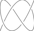
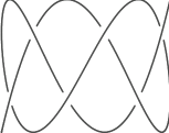
$4_{1}=C(2,2)$		$5_{1}=C(5)$

Figure 1. Polynomial representations of the knots $4_{1}$ and $5_{1}$

In particular this is why we prefer to consider our knots as long knots. As an application of Theorem 1.1, we determine in [BKP] the lexicographic degree of two-bridge knots of Conway’s normal form $C(m)$ with $m$ odd, or $C(m,n)$ with $mn$ positive and even.

The paper is organized as follows. In Section 2, we recall Conway’s notation for trigonal diagrams of two-bridge links, and their classification by their Schubert fractions. In Section 3 we define slide isotopies as trigonal isotopies such that the number of crossings never increases. We find necessary conditions for a two-bridge link diagram to be simple, that is to say it cannot be transformed into a simpler diagram by any slide isotopy. We use continued fraction properties to prove Theorem 1.1 in Section 4. In Section 5 we show that if a two-bridge link is neither a torus link nor a twist link, then it possesses awkward trigonal diagrams.

2. Trigonal diagrams of two-bridge knots

A two-bridge link admits a diagram in Conway’s open form (or trigonal form). This diagram, denoted by $D(m_{1},m_{2},\ldots,m_{k})$ where $m_{i}\in{\mathbb{Z}}^{*}$ are integers, is explained by the following picture (see [Co], [M, p. 187]).

\psfrag{a}{\small$m_{1}$}\psfrag{b}{\small$m_{2}$}\psfrag{c}{\small$m_{k-1}$}\psfrag{d}{\small$m_{k}$}\includegraphics{conway2.eps}

\psfrag{a}{\small$m_{1}$}\psfrag{b}{\small$m_{2}$}\psfrag{c}{\small$m_{k-1}$}\psfrag{d}{\small$m_{k}$}\includegraphics{conway3.eps}

Figure 2. Conway’s form for long links

The number of twists is denoted by the integer $\left|m_{i}\right|$, and the sign of $m_{i}$ is defined as follows: if $i$ is odd, then the right twist is positive, if $i$ is even, then the right twist is negative. In Figure 2 the $m_{i}$ are positive (the $m_{1}$ first twists are right twists). These diagrams are also called $3$-strand-braid representations, see [KL1, KL2].

The two-bridge links are classified by their Schubert fractions

$${\displaystyle{{\alpha}\overwithdelims. .{\beta}}}=m_{1}+{\displaystyle{{1}\overwithdelims. .{m_{2}+{\displaystyle{{1}\overwithdelims. .{\cdots+{\displaystyle{{1}\overwithdelims. .{m_{k}}}}}}}}}}=[m_{1},\ldots,m_{k}],\quad\alpha>0,\ (\alpha,\beta)=1.$$

Given $[m_{1},\ldots,m_{k}]={\displaystyle{{\alpha}\overwithdelims. .{\beta}}}$ and $[m^{\prime}_{1},\ldots,m^{\prime}_{l}]={\displaystyle{{\alpha^{\prime}}\overwithdelims. .{\beta^{\prime}}}}$, the diagrams $D(m_{1},m_{2},\ldots,m_{k})$ and $D(m^{\prime}_{1},m^{\prime}_{2},\ldots,m^{\prime}_{l})$ correspond to isotopic links if and only if $\alpha=\alpha^{\prime}$ and $\beta^{\prime}\equiv\beta^{\pm 1}\,(\hbox{\rm mod}\,\alpha)$, see [M, Theorem 9.3.3]. The integer $\alpha$ is odd for a knot, and even for a two-component link.

Any fraction admits a continued fraction expansion ${\displaystyle{{\alpha}\overwithdelims. .{\beta}}}=[m_{1},\ldots,m_{k}]$ where all the $m_{i}^{\prime}s$ have the same sign. Therefore every two-bridge link $K$ admits a diagram in Conway’s normal form, that is an alternating diagram of the form $D(m_{1},m_{2},\ldots m_{k})$ where all the $m_{i}^{\prime}s$ have the same sign. In this case we will write $L=C(m_{1},\ldots,m_{k}).$

It is classical that one can transform any trigonal diagram of a two-bridge link into its Conway’s normal form using the Lagrange isotopies, see [KL2] or [Cr, p.  204]:

(1) $$D(x,m,-n,-y)\rightarrow D(x,m-\varepsilon,\varepsilon,n-\varepsilon,y),\ \varepsilon=\pm 1,$$

where $m,n$ are integers, and $x,y$ are sequences of integers (possibly empty), see Figure 3.

\psfrag{a}{\small$m_{1}$}\psfrag{b}{\small$m_{2}$}\psfrag{c}{\small$m_{k-1}$}\psfrag{d}{\small$m_{k}$}\psfrag{a}{$m-1$}\psfrag{b}{$1-n$}\includegraphics{lag1.eps}   \psfrag{a}{\small$m_{1}$}\psfrag{b}{\small$m_{2}$}\psfrag{c}{\small$m_{k-1}$}\psfrag{d}{\small$m_{k}$}\psfrag{a}{$m-1$}\psfrag{b}{$1-n$}\psfrag{a}{$m-1$}\psfrag{b}{$n-1$}\includegraphics{lag3.eps}

Figure 3. Lagrange isotopies

These isotopies twist a part of the diagram, and the number of crossings may increase in intermediate diagrams. Since we want to simplify links without increasing their complexity, we introduce different isotopies in the following section.

3. Slide isotopies, simple and awkward diagrams

Definition 3.1.

We shall say that an isotopy of trigonal diagrams is a slide isotopy if the number of crossings never increases and if all the intermediate diagrams remain trigonal.

Example 3.2.

Some diagrams of the torus knot $5_{1}=C(5)$: $D(5)$, $D(2,1,-1,-2)$, $D(-1,-1,-1,1,1,1)$, $D(-2,2,-2,2)$, and $D(2,2,-1,2,2)$ are depicted in Figure 4. By Theorem 1.1, it is possible to simplify these diagrams into the alternating diagram $D(5)$ by slide isotopies only.

\psfrag{a}{\small$m_{1}$}\psfrag{b}{\small$m_{2}$}\psfrag{c}{\small$m_{k-1}$}\psfrag{d}{\small$m_{k}$}\includegraphics{tre-1.eps}

\psfrag{a}{\small$m_{1}$}\psfrag{b}{\small$m_{2}$}\psfrag{c}{\small$m_{k-1}$}\psfrag{d}{\small$m_{k}$}\includegraphics{tre-2.eps}

\psfrag{a}{\small$m_{1}$}\psfrag{b}{\small$m_{2}$}\psfrag{c}{\small$m_{k-1}$}\psfrag{d}{\small$m_{k}$}\includegraphics{tre-5.eps}

\psfrag{a}{\small$m_{1}$}\psfrag{b}{\small$m_{2}$}\psfrag{c}{\small$m_{k-1}$}\psfrag{d}{\small$m_{k}$}\includegraphics{tre-3.eps}

\psfrag{a}{\small$m_{1}$}\psfrag{b}{\small$m_{2}$}\psfrag{c}{\small$m_{k-1}$}\psfrag{d}{\small$m_{k}$}\includegraphics{tre-4.eps}

Figure 4. Some trigonal diagrams of the torus knot $5_{1}$

Remark 3.3.

(Göritz, 1934) Let $D$ be a trigonal diagram of a link $K$. Let $\widetilde{K}$ be the image of $K$ by a half-turn around the $x$-axis, and let $\widetilde{D}$ be the $xy$-projection of $\widetilde{K}$, see Figure 5.

\psfrag{a}{\small$m_{1}$}\psfrag{b}{\small$m_{2}$}\psfrag{c}{\small$m_{k-1}$}\psfrag{d}{\small$m_{k}$}\includegraphics{conway2.eps}

\psfrag{a}{\small$m_{1}$}\psfrag{b}{\small$m_{2}$}\psfrag{c}{\small$m_{k-1}$}\psfrag{d}{\small$m_{k}$}\includegraphics{conway4.eps}

Figure 5. The two diagrams $D$ and $\widetilde{D}$ with the same Conway notation.

The diagrams $D$ and $\widetilde{D}$ are diagrams of the same link $K,$ nevertheless they are generally not isotopic by a slide isotopy ([G]). It is often convenient to identify the diagrams $D$ and $\widetilde{D}.$

Definition 3.4.

We define the complexity of a trigonal diagram $D(m_{1},\ldots,m_{k})$ as $c(D)=k+\mathop{\sum}\limits\left|m_{i}\right|.$

Definition 3.5.

A trigonal diagram is called a simple diagram if it cannot be simplified into a diagram of lower complexity by using slide isotopies only. A non-alternating simple diagram is called an awkward diagram.

The next example shows the existence of awkward diagrams.

Example 3.6.

Let us consider the diagram $D=D(4,-3).$ It is an awkward diagram of the knot $6_{2}=C(3,1,2)$: the only possible Reidemeister moves increase the number of crossings. Of course, we can transform this diagram into an alternating one using Lagrange isotopies, but in this process some intermediate diagrams will have more crossings than $D$.

\psfrag{a}{\small$m_{1}$}\psfrag{b}{\small$m_{2}$}\psfrag{c}{\small$m_{k-1}$}\psfrag{d}{\small$m_{k}$}\includegraphics{d6_2-1.eps}		\psfrag{a}{\small$m_{1}$}\psfrag{b}{\small$m_{2}$}\psfrag{c}{\small$m_{k-1}$}\psfrag{d}{\small$m_{k}$}\includegraphics{d6_2-2.eps}
$D(4,-3)$		$6_{2}=C(3,1,2)$

Figure 6. $D(4,-3)$ is an awkward diagram of the knot $6_{2}=C(3,1,2)$

Remark 3.7.

More generally, let $m_{1},\ldots m_{k}$ be integers that are neither all positive nor all negative, and such that $|m_{i}|\geq 2$, $\left(|m_{1}|\geq 3\right.$ or $\left.m_{1}m_{2}>0\right)$ and $\left(|m_{k}|\geq 3\right.$ or $\left.m_{k-1}m_{k}>0\right).$ Then the diagram $D(m_{1},\ldots,m_{k})$ is awkward. In fact the only Reidemeister moves that can be applied increase the number of crossings. Kauffman and Lambropoulou call such diagrams hard diagrams, see [KL2].

Proposition 3.8.

Let $D=D(m_{1},\ldots,m_{k}),\ k>1$ be a simple trigonal diagram. Then we have

1. $\left|m_{1}\right|\geq 2$; $\left|m_{k}\right|\geq 2$; ${m_{i}}\neq 0,\ i=2,\ldots,k-1$;

2. $m_{1}m_{2}>0$ or $\left|m_{1}\right|\geq 3$; $\ m_{k-1}m_{k}>0$ or $\left|m_{k}\right|\geq 3$;

3. for $i=2,\ldots,k$, $m_{i-1}m_{i}\neq-1$;

4. suppose that $\left|m_{i}\right|=1$, then

   1. if $m_{i-1}m_{i}<0$, then $i\leq k-2$, $m_{i}m_{i+1}>0,$ and $m_{i}m_{i+2}>0$;

   2. if $m_{i}m_{i+1}<0$, then $i\geq 3$, $m_{i-2}m_{i}>0$, and $m_{i-1}m_{i}>0$.

Proof.

$(i)$ the slide isotopy $D(x,m,0)\rightarrow D(x)$ diminishes the complexity, consequently $m_{k}\neq 0,$ and similarly $m_{1}\neq 0.$ The slide isotopy $D(x,m,1)\rightarrow D(x,m+1)$ diminishes the complexity, see Figure 7.

\psfrag{a}{\small$m_{1}$}\psfrag{b}{\small$m_{2}$}\psfrag{c}{\small$m_{k-1}$}\psfrag{d}{\small$m_{k}$}\psfrag{m}{$m$}\psfrag{m+1}{$m+1$}\includegraphics{ni0-1.eps}

\psfrag{a}{\small$m_{1}$}\psfrag{b}{\small$m_{2}$}\psfrag{c}{\small$m_{k-1}$}\psfrag{d}{\small$m_{k}$}\psfrag{m}{$m$}\psfrag{m+1}{$m+1$}\includegraphics{ni0-2.eps}

Figure 7. The slide isotopy $D(x,m,1)\rightarrow D(x,m+1)$

Consequently $m_{k}\neq 1$ since $D$ is simple. We also have $m_{k}\neq-1,$ and similarly $m_{1}\neq\pm 1.$ The slide isotopy $D(x,m,0,n,y)\rightarrow D(x,m+n,y)$ shows that $m_{i}\neq 0.$

$(ii)$ Let us show that if $|m_{k}|=2$ then $m_{k}m_{k-1}>0$. Suppose on the contrary that, for example, $m_{k}=-2$ and $m_{k-1}>0$. Then the slide isotopy $D(x,m,-2)\rightarrow D(x,m-1,2)$ decreases the complexity of $D$, see Figure 8.

\psfrag{a}{\small$m_{1}$}\psfrag{b}{\small$m_{2}$}\psfrag{c}{\small$m_{k-1}$}\psfrag{d}{\small$m_{k}$}\psfrag{a}{$m-1$}\includegraphics{ni1-1.eps}   \psfrag{a}{\small$m_{1}$}\psfrag{b}{\small$m_{2}$}\psfrag{c}{\small$m_{k-1}$}\psfrag{d}{\small$m_{k}$}\psfrag{a}{$m-1$}\includegraphics{ni1-2.eps}

\psfrag{a}{\small$m_{1}$}\psfrag{b}{\small$m_{2}$}\psfrag{c}{\small$m_{k-1}$}\psfrag{d}{\small$m_{k}$}\psfrag{a}{$m-1$}\includegraphics{ni1-3.eps}

Figure 8. The slide isotopy $D(x,m,-2)\rightarrow D(x,m-1,2),\ m>0$

This contradicts the simplicity of $D$. Similarly, we see that if $|m_{1}|=2$ then $m_{1}m_{2}>0.$

$(iii)$ Consider the slide isotopy $D(x,m,-1,1,n,p,y)\rightarrow D(x,m-n,-1,1+p,y),$ see Figure 9. When $(p,y)=\emptyset$, this isotopy becomes $D(x,m,-1,1,n)\rightarrow D(x,m-n-1).$

\psfrag{a}{\small$m_{1}$}\psfrag{b}{\small$m_{2}$}\psfrag{c}{\small$m_{k-1}$}\psfrag{d}{\small$m_{k}$}\psfrag{a}{$m$}\psfrag{b}{$n$}\psfrag{c}{$p$}\includegraphics{ni2-1.eps}

\psfrag{a}{\small$m_{1}$}\psfrag{b}{\small$m_{2}$}\psfrag{c}{\small$m_{k-1}$}\psfrag{d}{\small$m_{k}$}\psfrag{a}{$m$}\psfrag{b}{$n$}\psfrag{c}{$p$}\psfrag{a}{$m$}\psfrag{b}{$-n$}\psfrag{c}{$p$}\includegraphics{ni2-2.eps}

\psfrag{a}{\small$m_{1}$}\psfrag{b}{\small$m_{2}$}\psfrag{c}{\small$m_{k-1}$}\psfrag{d}{\small$m_{k}$}\psfrag{a}{$m$}\psfrag{b}{$n$}\psfrag{c}{$p$}\psfrag{a}{$m$}\psfrag{b}{$-n$}\psfrag{c}{$p$}\psfrag{a}{$m-n$}\psfrag{b}{$p+1$}\includegraphics{ni2-3.eps}

Figure 9. The slide isotopy $D(x,m,-1,1,n,p,y)\rightarrow D(x,m-n,-1,1+p,y)$

It lowers the complexity, and consequently a simple diagram cannot be of the form $D(u,-1,1,v).$

$(iv)$ By $(i)$ we have $i\neq 1$ and $i\neq k$. Let us assume that $m_{i-1}m_{i}<0$, the proof in the case $m_{i}m_{i+1}<0$ being entirely similar. The slide isotopy $D(x,m,-1,n)\rightarrow D(x,m-1,-n+1)$ depicted in Figure 10 shows that $i\leq k-2$. Since $D$ is minimal, the slide isotopy $D(x,m,-1,n,p,y)\rightarrow D(x,m-1,-n,1,p-1,y)$ depicted in Figure 11 implies that $p<0,$ that is $m_{i}m_{i+2}>0$.

\psfrag{a}{\small$m_{1}$}\psfrag{b}{\small$m_{2}$}\psfrag{c}{\small$m_{k-1}$}\psfrag{d}{\small$m_{k}$}\psfrag{a}{$m-1$}\psfrag{b}{$n$}\includegraphics{ni3-1.eps}	\psfrag{a}{\small$m_{1}$}\psfrag{b}{\small$m_{2}$}\psfrag{c}{\small$m_{k-1}$}\psfrag{d}{\small$m_{k}$}\psfrag{a}{$m-1$}\psfrag{b}{$-n$}\includegraphics{ni3-2.eps}
\psfrag{a}{\small$m_{1}$}\psfrag{b}{\small$m_{2}$}\psfrag{c}{\small$m_{k-1}$}\psfrag{d}{\small$m_{k}$}\psfrag{a}{$m-1$}\psfrag{b}{$-n+1$}\includegraphics{ni3-3.eps}	\psfrag{a}{\small$m_{1}$}\psfrag{b}{\small$m_{2}$}\psfrag{c}{\small$m_{k-1}$}\psfrag{d}{\small$m_{k}$}\psfrag{a}{$m-1$}\psfrag{b}{$-n+1$}\includegraphics{ni3-4.eps}

Figure 10. The slide isotopy $D(x,m,-1,n)\mapsto D(x,m-1,-n+1)$, $m>0$

Now, assume that $m_{i}m_{i+1}<0$. Let $i$ be the maximal integer such that there exists a simple diagram $D(m_{1},\ldots m_{k})$ of length $k$ such that $\left|m_{i}\right|=1,\ m_{i-1}m_{i}<0,$ and $m_{i}m_{i+1}<0.$ Once more we use the slide isotopy $D(x,m,-1,n,p,y)\rightarrow D(x,m-1,-n,1,p-1,y)$ depicted in Figure 11. Since $p=m_{i+2}>0$ and $n=m_{i+1}>0$ by assumption, the new diagram contradicts the maximality of $i.$

\psfrag{a}{\small$m_{1}$}\psfrag{b}{\small$m_{2}$}\psfrag{c}{\small$m_{k-1}$}\psfrag{d}{\small$m_{k}$}\psfrag{a}{$m-1$}\psfrag{b}{$n$}\psfrag{c}{$p$}\includegraphics{ni5-1.eps}

\psfrag{a}{\small$m_{1}$}\psfrag{b}{\small$m_{2}$}\psfrag{c}{\small$m_{k-1}$}\psfrag{d}{\small$m_{k}$}\psfrag{a}{$m-1$}\psfrag{b}{$n$}\psfrag{c}{$p$}\psfrag{a}{$m-1$}\psfrag{b}{$-n$}\psfrag{c}{$p$}\includegraphics{ni5-2.eps}

\psfrag{a}{\small$m_{1}$}\psfrag{b}{\small$m_{2}$}\psfrag{c}{\small$m_{k-1}$}\psfrag{d}{\small$m_{k}$}\psfrag{a}{$m-1$}\psfrag{b}{$n$}\psfrag{c}{$p$}\psfrag{a}{$m-1$}\psfrag{b}{$-n$}\psfrag{c}{$p$}\psfrag{a}{$m-1$}\psfrag{b}{$-n$}\psfrag{c}{$p$}\includegraphics{ni5-3.eps}

Figure 11. The slide isotopy $D(x,m,-1,n,p,y)\rightarrow D(x,m-1,-n,1,p-1,y)$, $m>0$, $p<0$

$\Box$

The condition $(iv)$ of Proposition 3.8 asserts that a simple diagram cannot contain any subsequence $\pm(m,-1,n)$, $m,n>0$. Nevertheless, it can contain subsequences of the form $\pm(m,-1)$, $m>1$. However, the next corollary shows that this phenomenon can be avoided.

Corollary 3.9.

Let $D$ be a trigonal Conway diagram of a two-bridge link. Then it is possible to transform $D$ by slide isotopies into a simple diagram $D(m_{1},\ldots,m_{k})$ such that for $i=2,\ldots,k$, either $\left|m_{i}\right|\neq 1,\$ or $m_{i-1}\,m_{i}>0$.

Proof. Let us suppose that each simple diagram deduced from $D$ by slide isotopies contains subsequences of the form $\pm(m,-1),\ m\geq 2,$ and let $\mu\neq 0$ be the minimum number of such subsequences.

Among all simple diagrams $D(m_{1},\ldots,m_{k})$ deduced from $D$ by slide isotopies and possessing $\mu$ such subsequences there is a minimal integer $r$ such that $(m_{r-1},m_{r})=\pm(m,-1),\ m\geq 2$. By Proposition 3.8, $(iv)$ we have $r\leq k-2$ and our diagram is of the form $\Delta=D(x,m,-1,n,p,y)$, where $n,p<0$. The use of the slide isotopy depicted in Figure 11: $\Delta\rightarrow\Delta^{\prime}=D(x,m-1,-n,1,p-1,y)$, contradicts the minimality of either $\mu$ or $r$. $\Box$

4. Proof of Theorem 1.1

The proof is based on some arithmetical properties of the continued fractions $[m_{1},\ldots,m_{k}]$ related to simple diagrams $D(m_{1},\ldots,m_{k})$, that are consequences of Proposition 3.8 and Corollary 3.9.

Lemma 4.1.

Let $x$ be a rational number defined by its continued fraction expansion $x={\displaystyle{{\alpha}\overwithdelims. .{\beta}}}=[m_{1},m_{2},\ldots,m_{k}]$, $m_{1}>0$, $|m_{k}|\geq 2$, $m_{i}\in{\bf Z}^{*}$, $\alpha\geq 0$. Suppose that for $i=2,\ldots,k$, we have either $|m_{i}|\neq 1$ or $m_{i-1}m_{i}>0.$ Then the following hold:

• $x>m_{1}-1,$ and consequently $\alpha>0$ and $\beta>0$;

• if $k\geq 2$ and ($m_{k-1}m_{k}>0$ or $\left|m_{k}\right|\geq 3$), then $\alpha\geq 2$ and $\beta\geq 2$;

• if in addition we have $m_{1}\geq 2$ and $(m_{1}m_{2}>0$ or $m_{1}\geq 3)$ then $x>2$;

• if in addition we have $k\geq 3$ and $(\left|m_{2}\right|\neq 1$ or $m_{2}m_{3}>0),$ then $\alpha\not\equiv 1\,(\hbox{\rm mod}\,\beta).$

Proof.

$(a)$ We use an induction on $k$. If $k=1,$ then we have $x=m_{1}>m_{1}-1,$ and the result is true. Let us suppose that $k\geq 2.$ If $m_{2}>0,$ then we have $y=[m_{2},\ldots,m_{k}]>0,$ and then $x=m_{1}+1/y>m_{1}>m_{1}-1.$ If $m_{2}<0,$ then by assumption $-m_{2}\geq 2$. By induction we have $y=[-m_{2},\ldots,-m_{k}]>1,$ and then $x=m_{1}-1/y>m_{1}-1.$

$(b)$ We use again an induction on $k$. If $k=2$, then there are two cases to consider.

If $m_{2}>0,$ then we have $\beta=m_{2}\geq 2,$ and $\alpha=m_{1}m_{2}+1\geq 2.$

If $m_{2}<0,$ then we have $\left|m_{2}\right|\geq 3.$ Then $\beta=|m_{2}|\geq 3$ and $\alpha=m_{1}|m_{2}|-1\geq 3m_{1}-1\geq 2.$

Let us suppose now that $k\geq 3.$ Let $x=m_{1}+q/p,$ where $p/q=[m_{2},\ldots,m_{k}],\ p>0.$

If $m_{2}>0$, then $\beta=p\geq 2$ and $q\geq 2$ by induction, and then $\alpha=m_{1}p+q\geq 2.$

If $m_{2}<0,$ then $-m_{2}\geq 2.$ By induction, $[-m_{2}-1,-m_{3},\ldots,-m_{k}]={\displaystyle{{p+q}\overwithdelims. .{-q}}}$ is such that $p+q\geq 2$ and $-q\geq 2.$ Consequently, we obtain $\beta=p\geq 2-q\geq 4\geq 2,$ and $\alpha=m_{1}p+q=m_{1}(p+q)+(m_{1}-1)(-q)\geq 2m_{1}\geq 2.$

$(c)$ If $m_{2}>0,$ then $x>m_{1}\geq 2.$ If $m_{2}<0,$ then $m_{1}\geq 3,$ and then $x>m_{1}-1\geq 2$ by $(a).$

$(d)$ If $m_{2}<0,$ then $-m_{2}\geq 2$ and as in the proof of $(b)$ we get $p+q\geq 2$ and $-q\geq 2$, where ${\displaystyle{{p}\overwithdelims. .{-q}}}=[-m_{2},\ldots,-m_{k}]>1.$ Consequently we obtain $p\geq 2-q>1-q>0$ and then $q\not\equiv 1\ \,(\hbox{\rm mod}\,p).$ As $\alpha=m_{1}p+q$ and $\beta=p,$ the result is proved in this case.

Suppose now that $m_{2}>0$, and consider ${\displaystyle{{u}\overwithdelims. .{v}}}=[m_{3},\ldots,m_{k}]$ with $u>0$. In particular, we have $\beta=m_{2}u+v$, and $\alpha=m_{1}\beta+u\equiv u\ \,(\hbox{\rm mod}\,\beta)$.

If $m_{3}>0$, then $v>0$ and so $\beta>u$. If $k=3,$ then $u=m_{3}\geq 2.$ If $k>3,$ then we have $u\geq 2$ by $(b).$ Hence $\beta>u\geq 2,$ and so $\alpha\equiv u\not\equiv 1\ \,(\hbox{\rm mod}\,\beta).$

If $m_{3}<0,$ then $m_{2}\geq 2$, $-m_{3}\geq 2$, and $v<0$. We have ${\displaystyle{{u}\overwithdelims. .{-v}}}>1$ by $(a),$ i.e. $u>-v$. Hence we have $\beta\geq 2u+v>u\geq 2,$ and we obtain $\alpha\equiv u\not\equiv 1\ \,(\hbox{\rm mod}\,\beta).$ $\Box$

Proof of Theorem 1.1. Let $D(m_{1},\ldots,m_{k})$ be a simple diagram deduced from $D$ by admissible isotopies, and satisfying the condition of Corollary 3.9. Recall that it also satisfies all conclusions of Proposition 3.8. We write ${\displaystyle{{\alpha}\overwithdelims. .{\beta}}}=[m_{1},m_{2},\ldots,m_{k}]$ with $\alpha>0$ and $(\alpha,\beta)=1$. Without loss of generality, we may assume that both $m$ and $n$ are nonnegative.

Let us first consider the case when $K$ is the torus link $C(m)$. By the classification of torus links by their Schubert fractions, we have $\alpha=m$ and $\beta=1\,(\hbox{\rm mod}\,m)$. If $k\geq 2$, then Lemma 4.1 $(b)$ implies that $|\beta|\geq 2$ so $\left|\beta\right|\geq m-1$. But then, by Lemma 4.1 $(c)$, we would have $\alpha=m>2|\beta|\geq 2m-2$ so $m\leq 1$. Hence we obtain $k=1$, which proves the result.

Now, let us consider the case when $K$ is the twist link $C(m,n)$ with $m\geq 2$ and $n\geq 2$. Then we have $\alpha=mn+1$, and either $\beta\equiv n\,(\hbox{\rm mod}\,\alpha)$ or $\beta\equiv-m\,(\hbox{\rm mod}\,\alpha)$. Lemma 4.1 $(c)$ implies that $\alpha>2|\beta|$, from which we deduce that $\beta=n$ or $\beta=-m$. Consequently we have $\alpha\equiv 1\,(\hbox{\rm mod}\,\beta)$, which implies by Lemma 4.1 $(d)$ that $k=2$.

By Proposition 3.8 $(i)$, we have $|m_{1}|\geq 2$ and $|m_{2}|\geq 2$. If $m_{1}m_{2}<0,$ then we would have ${\displaystyle{{\alpha}\overwithdelims. .{\beta}}}={\displaystyle{{|m_{1}m_{2}|-1}\overwithdelims. .{\pm m_{2}}}}$. In particular we would have $\alpha\equiv-1\,(\hbox{\rm mod}\,\beta),$ which is impossible since $\alpha\equiv 1\,(\hbox{\rm mod}\,\beta)$ and $|\beta|=|m_{2}|\geq 3$ by Proposition 3.8 $(ii)$. Consequently we have $m_{1}m_{2}>0$ and the diagram is alternating. $\Box$

5. Some awkward trigonal diagrams

The following result shows that if a two-bridge link is not of the Conway normal form $C(m)$, or $C(m,n)$ with $mn>0$, then it possesses an awkward trigonal diagram.

Proposition 5.1.

Let $k\geq 3$ and let $K$ be a two-bridge link of Conway normal form $C(m_{1},\ldots,m_{k})$, $m_{i}>0$, $m_{1}\geq 2,$ $m_{k}\geq 2.$ Then $K$ possesses an awkward trigonal diagram.

Proof. Let $[m_{k-2},m_{k-1},m_{k}]=[m,a,n]$. Using the Lagrange identity we have $[m,a,n]=[m+1,-1,1-a,-n]$. If $a=1$, then this last continued fraction is $[m+1,-n-1]$. Therefore $K$ admits the trigonal diagram

• $D(m_{1},\ldots,m_{k-3},m+1,-1,1-a,-n)$, if $a>1$;

• $D(m_{1},\ldots,m_{k-3},m+1,-n-1)$ if $a=1$.

These two diagrams are awkward (see Figure 12). $\Box$

\psfrag{a}{\small$m_{1}$}\psfrag{b}{\small$m_{2}$}\psfrag{c}{\small$m_{k-1}$}\psfrag{d}{\small$m_{k}$}\psfrag{a}{$m$}\psfrag{b}{$1-a$}\psfrag{c}{$-n$}\includegraphics{awk1.eps}

\psfrag{a}{\small$m_{1}$}\psfrag{b}{\small$m_{2}$}\psfrag{c}{\small$m_{k-1}$}\psfrag{d}{\small$m_{k}$}\psfrag{a}{$m$}\psfrag{b}{$1-a$}\psfrag{c}{$-n$}\psfrag{a}{$m$}\psfrag{b}{$1-a$}\psfrag{c}{$-n$}\includegraphics{awk2.eps}

Figure 12. The awkward diagrams $D(x,m+1,-1,1-a,-n)$ and $D(x,m+1,-n-1)$.

Furthermore, we have a stronger result.

Theorem 5.2.

Let $k\geq 3$ and let $K$ be a two-bridge link of Conway normal form $C(m_{1},\ldots,m_{k})$, $m_{i}>0$, $m_{1}\geq 2,$ $m_{k}\geq 2.$ Then $K$ possesses a hard trigonal diagram.

Proof. Using the identity ${\displaystyle{{az+1}\overwithdelims. .{(a-1)z+1}}}=[\underbrace{2,-2,2,\ldots,(-1)^{a-2}2}_{a-1\hbox{ \scriptsize terms}},(-1)^{a-1}(z+1)]$, we obtain

$$[m,a,n]=[m+1,-{\displaystyle{{an+1}\overwithdelims. .{(a-1)n+1}}}]=[m+1,-2,2,-2,\ldots,(-1)^{a-1}2,(-1)^{a}(n+1)],$$

and we deduce that

$$[m_{1},\ldots,m_{k}]=[x,m,a,n]=[x,m+1,-2,2,\ldots,(-1)^{a-1}2,(-1)^{a}(n+1)].$$

Therefore, the diagram $D=D(x,m+1,-2,2,\ldots,(-1)^{a-1}2,(-1)^{a}(n+1))$ is a diagram of $K$, and it is a hard diagram by Remark 3.7. $\Box$

Remark 5.3.

Theorem 1.1 shows that the trivial knot has no trigonal awkward diagram. On the other hand, Göritz found an awkward diagram of the trivial knot in [G], and Kauffman and Lambropoulou constructed many such examples (see [KL2, A, Cr]).

 

Erwan Brugallé
École Polytechnique, Centre Mathématiques Laurent Schwartz, 91 128 Palaiseau Cedex, France
e-mail: erwan.brugalle@math.cnrs.fr

Pierre-Vincent Koseleff
Université Pierre et Marie Curie (UPMC Sorbonne Universités),
Institut de Mathématiques de Jussieu (IMJ-PRG) & Inria-Rocquencourt
e-mail: koseleff@math.jussieu.fr

Daniel Pecker
Université Pierre et Marie Curie (UPMC Sorbonne Universités),
Institut de Mathématiques de Jussieu (IMJ-PRG),
e-mail: pecker@math.jussieu.fr

References

- [A] C. C. Adams, The Knot Book: an Elementary introduction to the Mathematical Theory of Knots, American Mathematical Society, Providence. 2004.
- [BKP] E. Brugallé, P. -V. Koseleff, D. Pecker, On the lexicographic degree of two-bridge knots (2014)
- [Co] J. H. Conway, An enumeration of knots and links, and some of their algebraic properties, Computational Problems in Abstract Algebra (Proc. Conf., Oxford, 1967), 329–358 Pergamon, Oxford (1970)
- [Cr] P. R. Cromwell, Knots and links, Cambridge University Press, Cambridge, 2004. xviii+328 pp.
- [G] L. Göritz, Bemerkungen zur Knoten theorie, Abhandlungen Math. Seminar Univ. Hamburg, Vol 10 201-210, (1934)
- [KL1] L. H. Kauffman, S. Lambropoulou, On the classification of rational knots, L’Enseignement Mathématique, 49, 357-410, (2003)
- [KL2] L. H. Kauffman, S. Lambropoulou, Hard unknots and collapsing tangles, Introductory lectures on knot theory, Ser. Knots Everything, 46, World Sci. Publ., Hackensack, 187-247, (2012)
- [KP1] P. -V. Koseleff, D. Pecker, On polynomial Torus Knots, Journal of Knot Theory and its Ramifications, Vol. 17 (12) (2008), 1525-1537
- [KP2] P. -V. Koseleff, D. Pecker, Chebyshev knots, Journal of Knot Theory and Its Ramifications, Vol 20, 4 (2011) 1-19
- [M] K. Murasugi, Knot Theory and its Applications, Boston, Birkhäuser, 341p., 1996.
- [RS] A. Ranjan and R. Shukla, On polynomial representation of torus knots, Journal of knot theory and its ramifications, Vol. 5 (2) (1996) 279-294.
- [V] V. A. Vassiliev, Cohomology of knot spaces, Theory of singularities and its Applications, Advances Soviet Maths Vol 1 (1990)