Exceptional points for parameter estimation in open quantum systems: Analysis of the Bloch equations

Abstract

We suggest to employ the dissipative nature of open quantum systems for the purpose of parameter estimation: The dynamics of open quantum systems is typically described by a quantum dynamical semigroup generator ${\cal L}$. The eigenvalues of ${\cal L}$ are complex, reflecting unitary as well as dissipative dynamics. For certain values of parameters defining ${\cal L}$, non-hermitian degeneracies emerge, i.e. exceptional points ($EP$). The dynamical signature of these EPs corresponds to a unique time evolution. This unique feature can be employed experimentally to locate the EPs and thereby to determine the intrinsic system parameters with a high accuracy. This way we turn the disadvantage of the dissipation into an advantage. We demonstrate this method in the open system dynamics of a two-level system described by the Bloch equation, which has become the paradigm of diverse fields in physics, from NMR to quantum information and elementary particles.

1 Introduction

Felix Bloch [1] pioneered the dynamical description of open quantum systems. Originally Bloch’s equations describe the relaxation and dephasing of a nuclear spin in a magnetic field. Soon it became apparent that the treatment can be extended to a generic two-level-system (TLS), such as the dynamics of laser driven atoms in the optical regime [2, 3, 4]. The open TLS has been used to model many different fields of physics. The TLS or a q-bit is at the foundation of quantum information [5, 6, 7, 8, 9]. In particle physics the TLS algebra has been employed in studies of possible deviations from quantum mechanics in the context of neutrino oscillations [10], as well as quantum entanglement [11, 12, 13, 14, 15], associated with electron/positron collisions and entangled systems due to EPR-Bell correlations [16].

The TLS is the base for setting the frequency standard for atomic clocks [17]. As a result accurate measurement of frequency is an important issue. Quantum-enhanced measurements based on interferometry have been suggested as means to beat the shot noise limit [18]. In these methods the decoherence rate is the limiting factor [19]. In some cases quantum error correction can increase the coherence time and the accuracy [20]. In the present study we want to suggest an opposite strategy. By employing the non-hermitian character of the dynamics, the decoherence can be transformed from a bug to a feature.

2 Exceptional points in open quantum systems

The Bloch equation is the simplest example of a quantum Master equation. Bloch rederived the equation from first principles, employing the assumption of weak coupling between the system and bath [21, 22]. These studies have paved the way for a general theory of quantum open systems. Davies [23] rigorously derived the weak coupling limit, resulting in a quantum Master equation which leads to a completely positive dynamical semigroup [24]. Based on a mathematical construction, Lindblad and Gorini, Kossakowski and Sudarshan (L-GKS) obtained the general structure of the generator ${\cal L}$ of a completely positive dynamical semigroup [25, 26]. In the Heisenberg representation the L-GKS generator becomes [27, Chapter 3]:

$$\frac{d}{dt}{\bm{\mathrm{\hat{X}}}}~{}=~{}\frac{\partial{\bm{\mathrm{\hat{X}}}}}{\partial t}+i\left[{\bm{\mathrm{\hat{H}}}},{\bm{\mathrm{\hat{X}}}}\right]+\sum_{k}\left({\bm{\mathrm{\hat{V}}}}_{k}^{\dagger}{\bm{\mathrm{\hat{X}}}}{\bm{\mathrm{\hat{V}}}}_{k}-\frac{1}{2}\left[{\bm{\mathrm{\hat{V}}}}_{k}^{\dagger}{\bm{\mathrm{\hat{V}}}}_{k},{\bm{\mathrm{\hat{X}}}}\right]_{+}\right).$$ (1)

where ${\bm{\mathrm{\hat{X}}}}$ is an arbitrary operator. The hamiltonian ${\bm{\mathrm{\hat{H}}}}$ is hermitian and operators ${\bm{\mathrm{\hat{V}}}}_{k}$ are defined to operate in the Hilbert space of the system. The $\left[\cdot,\cdot\right]_{+}$ denotes an anti commutator.

The set of operators $\{{\bm{\mathrm{\hat{X}}}}\}$ supports a Hilbert space construction using the scalar product: $({\bm{\mathrm{\hat{X}}}}_{1},{\bm{\mathrm{\hat{X}}}}_{2})\equiv tr\{{\bm{\mathrm{\hat{X_{1}}}}}^{\dagger}{\bm{\mathrm{\hat{X_{2}}}}}\}$. A crucial simplification to Eq. (1) is obtained when a set of operator is closed to the generator $\cal{L}$. Then we can rephrase the dynamics with a matrix-vector notation [28]:

$$\dot{\vec{Y}}=M\vec{Y}$$ (2)

where $\vec{Y}$ is the vector of basis operators and $M$ is the representation of the generator ${\cal L}$ in this vector space. The eigenvalues of the matrix $M$ reflect the non-hermitian dynamics generated by ${\cal L}$. In general they are complex with the steady state eigenvector having an eigenvalue of zero. The solution for this equation is:

$$\vec{Y}(t)=e^{Mt}\vec{Y}(0).$$

When $M$ is diagonalizable, we can write $M=T\Lambda T^{-1}$, for a non-singular matrix $T$ and a diagonal matrix $\Lambda$, which has the eigenvalues $\{\lambda_{i}\}$ on the diagonal. Then we have $e^{Mt}=Te^{\Lambda t}T^{-1}$, with the diagonal matrix $e^{\Lambda t}$, which has the exponential of the eigenvalues, $e^{\lambda_{i}t}$, on its diagonal. The resulting dynamics of expectation values of operators, as well as other correlation functions, follows a sum of decaying oscillatory exponentials. The analytical form of such dynamics is:

$$\left\langle X(t)\right\rangle=\sum_{k}\;d_{k}\exp[-i\omega_{k}t]\;,$$ (3)

where $-i\omega_{k}$, denoted as complex frequencies, are the eigenvalues of $M$, $d_{k}$ are the associated amplitudes, and both $\omega_{k}$ and $d_{k}$ can be complex. The real part of the complex frequency $\omega_{k}$ represents the oscillation rate, while the imaginary part, $Im(\omega_{k})\leq 0$ represents the decaying rate,

For special values of the system parameters the spectrum of the non-hermitian matrix $M$ is incomplete. This is due to the coalescence of several eigenvectors, referred to as a non-hermitian degeneracy. The difference between hermitian degeneracy and non-hermitian degeneracy is essential: In the hermitian degeneracy, several different orthogonal eigenvectors are associated with the same eigenvalue. In the case of non-hermitian degeneracy several eigenvectors coalesce to a single eigenvector [29, Chapter 9]. As a result, the matrix $M$ is not diagonalizable.

The exponential of a non-diagonalizable matrix $M$ can be expressed using its Jordan normal form: $M=TJT^{-1}$. Here, $J$ is a Jordan-blocks matrix which has (at least) one non-diagonal Jordan block; $J_{i}=\lambda_{i}I+N$, where $I$ is the identity and $N$ has ones on its first upper off-diagonal. The exponential of $M$ is expressed as $e^{Mt}=Te^{Jt}T^{-1}$, with the block-diagonal matrix $e^{Jt}$, which is composed from the exponential of the Jordan blocks $e^{J_{i}t}$. For non-hermitian degeneracy of an eigenvalue $\lambda_{i}$, the exponential of the block $J_{i}$ will have the form: $e^{J_{i}t}=e^{\lambda_{i}It+Nt}=e^{\lambda_{i}t}e^{Nt}.$ The matrix $N$ is nilpotent and therefore the Taylor series of $e^{Nt}$ is finite, resulting in a polynomial in the matrix $Nt$. This gives rise to a polynomial behaviour of the solution, and the dynamics of expectation values will have the analytical form of

$$\left\langle X(t)\right\rangle=\sum_{k}\sum_{\alpha=0}^{r_{k}}\;{d}_{k,\alpha}t^{\alpha}\exp[-i\omega_{k}^{(r_{k})}t]\;,$$ (4)

replacing the form of Eq. (3). Here, $\omega_{k}^{(r_{k})}$ denotes an eigenvalue with multiplicity of $r_{k}+1$. Note that for non-degenerate eigenvalues, i.e. $r_{k}=0$, we have $d_{k,0}=d_{k}$ and $\omega_{k}^{(0)}=\omega_{k}$. The difference in the analytic behaviour of the dynamics results in non-Lorentzian line shapes, with higher order poles in the complex spectral domain.

The point in the spectrum where the eigenvectors coalesce is known as an exceptional point ($EP$). When two eigenvalues of the master equation coalesce into one, a second-order non-hermitian degeneracy is obtained. We refer to it as EP2, while a third-order non-hermitian degeneracy is denoted by EP3.

This study addresses the scenario of the dynamics of a system coupled to a bath. The formalism is a reduced description of a tensor product of the system and the bath [27, 30]. The coupling to the bath introduces dissipation and dephasing into the dynamics. The state is represented as a density operator in Liouville space, and the dynamics is governed by the L-GKS equation. The non hermitian properties of the dynamical generator ${\cal L}$ is caused by tracing out the bath degrees of freedom. We employ the Heisenberg picture with a complete operator basis set in Liouville space.

Previous studies of the physics of EPs investigated the scenario of scattering resonances phenomena. In that different scenario, the non hermitian properties of the effective Hamiltonian are caused by the interaction between the discrete states via the common continuum of the scattering states [31, 32]. In those studies only coherent dynamics is considered and the dissipation and dephasing phenomena are absent.

Examples for EPs have been described in optics [33, 34], in atomic physics [35, 36, 37, 38, 39, 40], in electron-molecule collisions [41], superconductors [42], quantum phase transitions in a system of interacting bosons [43], electric field oscillations in microwave cavities [44], in PT-symmetric waveguides [45], and in mesoscopic physics [46, 47].

Recently, Wiersig suggested a method to enhance the sensitivity of detectors using exceptional points [48]. Below we suggest to employ the exceptional points for the purpose of parameter estimation.

3 Identifying the exceptional points and parameter estimation

The analytical form of decaying exponentials, Eq. (3), is used in harmonic inversion methods to find the frequencies and amplitudes of the time series signal [49, 50, 51]. These frequencies and amplitudes can be employed to estimate the system parameters. If the sensitivity of the estimated frequencies is increased with respect to the system controls, the accuracy of the parameter estimation is enhanced. Such sensitivity increase can be achieved using the special character of the dynamics at exceptional points.

At exceptional points the analytical form includes also polynomials (Eq. (4)). Fuchs et al. showed that applying the standard harmonic inversion methods to a signal generated by Eq. (4) leads to divergence of the amplitudes $d_{k}$. An extended harmonic inversion method can fix the problem. The divergence of the amplitudes $d_{k}$ at the vicinity of exceptional point can be used to locate them in the parameter space very accurately [52]. This is a consequence of the special non analytic character close to the EP (Cf. in Chapter 9 in Ref. [29]).

Relying on the ability to accurately locate the EPs in the parameter space, we suggest to use the EPs for parameter estimation. The procedure we suggest follows:

1. Accurately locate in the parameter space the desired exceptional point by iterating the following steps:

   1. Perform the experiment to get a time series of an observable for example the polarization as a function of time.

   2. Obtain the characteristic frequencies and amplitudes of the signal using harmonic inversion methods.

   3. In the parameter space, estimate the direction and distance to the EP and determine new parameters for the next iteration.

2. Invert the relations between the characteristic frequencies and the system parameters at the EP to obtain the system parameters.

The accurate location of the exceptional points, followed by inverting the relations, will lead to accurate parameter estimation.

4 Determination of the physical parameters in two level systems

4.1 The Bloch equation

The Bloch equation describes the dynamics of the three components of the nuclear spin, $S_{x}$, $S_{y}$, and $S_{z}$, under the influence of an external magnetic field, or a two-level atom in external electromagnetic field. In the rotating frame, we can write the equations in a matrix-vector notation:

$$\frac{d}{dt}\left(\begin{array}[]{c}\tilde{S}_{x}\\ \tilde{S}_{y}\\ S_{z}\end{array}\right)=\left(\begin{array}[]{ccc}-\frac{1}{T_{2}}&\Delta&0\\ -\Delta&-\frac{1}{T_{2}}&\epsilon\\ 0&-\epsilon&-\frac{1}{T_{1}}\end{array}\right)\left(\begin{array}[]{c}\tilde{S}_{x}\\ \tilde{S}_{y}\\ S_{z}\end{array}\right)+\left(\begin{array}[]{c}0\\ 0\\ \frac{1}{T_{1}}S_{z}^{0}\end{array}\right),$$ (17)

with $T_{1}$ and $T_{2}$ as the dissipation and dephasing relaxation parameters, and the detuning from resonance $\Delta$ and the amplitude $\epsilon$ as the field parameters. See details in A.

The Bloch equations can be derived from the L-GKS equation of the two-level system, with the effective rotating-frame Hamiltonian

$${\bm{\mathrm{\hat{H}}}}=\Delta{\bm{\mathrm{\hat{S}}}}_{z}+\epsilon{\bm{\mathrm{\hat{\tilde{S}}}}}_{x},$$

along with relaxation and dephasing terms. See B for details. Reducing the number of parameters, the Master equation can be incorporated in the matrix:

$$\text{M}=\left(\begin{array}[]{ccc}-\frac{\Gamma}{2}&\Delta&0\\ -\Delta&-\frac{\Gamma}{2}&\epsilon\\ 0&-\epsilon&\text{-$\Gamma$}\end{array}\right),$$ (18)

with $\Gamma=\frac{3}{2}\frac{1}{T_{1}}-\frac{1}{T_{2}}$ as the general relaxation coefficient (See B).

The dynamics is determined by the exponential $e^{Mt}$, which typically describes oscillating decaying signal, Cf. Eq. (3). Nevertheless, for specific parameters leading to EP the dynamics is modified to include polynomials, Cf. Eq. (4).

4.2 Exceptional points in the Bloch equation

The EPs are non-hermitian degeneracies in the matrix $M$ of Eq. (18). The task is to express the EPs using the parameters of this matrix. Explicit derivations are presented in C. Non-hermitian degeneracies of the eigenvalues [29], EP2, occur when

$$\Gamma^{4}\Delta^{2}+16\left(\Delta^{2}+\epsilon^{2}\right)^{3}+\Gamma^{2}\left(8\Delta^{4}-20\Delta^{2}\epsilon^{2}-\epsilon^{4}\right)=0.$$

Figure 1 shows a map of EP2 curve as a function of $\epsilon$ and $\Delta$ for fixed $\Gamma=0.1$. Such figures were obtained in the study of analytical solutions for the Bloch equation [53, 54, 55].

A third order exceptional point, EP3, occurs when $\Delta=\pm\sqrt{1/108}\,\Gamma$, $\epsilon=\sqrt{8/108}\,\Gamma$ (red asterisks in Figure 1). These triple-degeneracies EP3 occur twice, and have a cusp-like behaviour, emerging from the EP2-curves, identifiable as a section through an elliptic umbilic catastrophe [56]. This topology is also consistent with an analysis of non hermitian degeneracies in a two-parameters family of $3\times 3$ matrices [57]. In very strong driving fields the matrix $M$ will loose symmetry [58, 59] maintaining the cusps but skewing the topology.

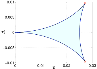
Figure 1: A map of the non-hermitian degeneracies of the eigenvalues of the matrix $M$ of Eq. (18), as a function of $\epsilon$ and $\Delta$, for fixed $\Gamma=0.1$. The lines represent second order exceptional points (EP2). The cusps, where $\Delta=\pm\sqrt{1/108}\,\Gamma$, $\epsilon=\sqrt{8/108}\,\Gamma$ (red asterisks), are third order exceptional point (EP3). In the area inside the "triangle", marked with pale blue, the eigenvalues of the matrix M are real. The EP2 curve distinguishes between points with real and complex eigenvalues.

4.3 EP identification and parameter estimation

We now describe the two steps of the method for accurate determination the physical parameters. The first step is to identify the desired exceptional point using a sequence of measured time-dependent signals. The second step is to invert the relations and determine the system parameters.

4.3.1 Identifying the second and third order exceptional points

To identify the exceptional points we used time series of the polarization observable $S_{z}\equiv\langle{\bm{\mathrm{\hat{S}}}}_{z}\rangle$, initially at the ground state. We simulated the dynamics with varying field parameters ($\epsilon$, $\Delta$) generating a time series of polarization $S_{z}[n]=S_{z}(n\delta t)$. This signals served as the input for the harmonic inversion.

The parameters $\Delta$ and $\epsilon$ were tuned close to an EP. Generically we should have

$$S_{z}(t)=d_{1}e^{-i\omega_{1}t}+d_{2}e^{-i\omega_{2}t}+d_{3}e^{-i\omega_{3}t},$$

but in the EP2 $(r_{k}=1)$ we get

$$S_{z}(t)=d_{1}e^{-i\omega_{1}t}+\left(d_{2,0}+d_{2,1}t\right)e^{-i\omega_{2}^{(1)}t},$$

and for EP3 $(r_{k}=2)$

$$S_{z}(t)=\left(d_{1,0}+d_{1,1}t+d_{1,2}t^{2}\right)e^{-i\omega_{1}^{(2)}t}.$$

(Cf. Eqs. (3) and (4)). We located suspected EPs by identifying possible degeneracies of the assigned frequencies $\omega_{k}$. As stated earlier, applying standard harmonic inversion methods for the time series generated by a non-diagonalizable matrix, leads to divergence of the amplitudes $d_{k}$ [52]. This divergence can be used to locate the exceptional points accurately. A verification can be obtained by using the extended harmonic inversion method.

This procedure was employed to identify an EP2 for fixed $\Gamma=0.1$ and $\epsilon=0.01$, with varying $\Delta$. The purple asterisks at Fig. 2 displays the absolute value of the difference between the frequencies $|\omega_{2}-\omega_{1}|$, obtained by the harmonic inversion for each parameter set. The degeneracy point is clearly observed. The diverging behaviour of the amplitudes is shown in red stars. It is consistent with the degeneracy of the frequencies. The EP2 is located at $\Delta=1.021\times 10^{-3}$, consistent with the prediction. Using a finer mesh of sampling points the EP can be identified with a resolution exceeding $0.5\times 10^{-9}$.

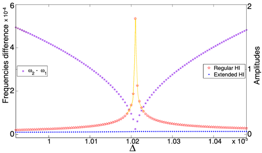
Figure 2: Identifying an EP2 for $\Gamma=0.1$ and $\epsilon=0.01$. The left y-axis (purple asterisks) shows the absolute value of the difference between the frequencies, $|\omega_{2}-\omega_{1}|$, versus the detuning $\Delta$. The non-hermitian degeneracy point is located with high resolution. The right y-axis shows the corresponding amplitude, obtained by the regular harmonic inversion method $|d_{1}|$ (red stars), and by the extended method $|d_{1,0}|$ (blue points). The diverging behaviour of $|d_{1}|$ indicates that the degeneracy is an EP.

The EP3 was identified by a 2-D search performed by varying $\epsilon$ and $\Delta$, for fixed $\Gamma=0.1$. We searched for the degeneracies of the three eigenvalues by employing the 2-D function

$$F(\Delta,\epsilon,\Gamma)=\log\left(\left|\frac{1}{(\omega_{1}-\omega_{2})}\frac{1}{(\omega_{2}-\omega_{3})}\frac{1}{(\omega_{3}-\omega_{1})}\right|\right),$$ (19)

which should diverges at the EP curve. Numerically, we get high values at this curve, with highest values obtained at the EP3. The upper panel of Figure 3 shows the sharp curve of peaks following the curve of exceptional points. The highest point on the merging two ridges is the EP3. The lower panel of Figure 3 shows the sum of the absolute values of the amplitudes, calculated by the standard harmonic inversion. The curve of the exceptional points is clearly identified.

Refining the search leads to very high resolution, and the EP3 can be identified with a high accuracy, approaching the theoretical values of $\Delta=\sqrt{1/108}\,\Gamma$, $\epsilon=\sqrt{8/108}\,\Gamma$.

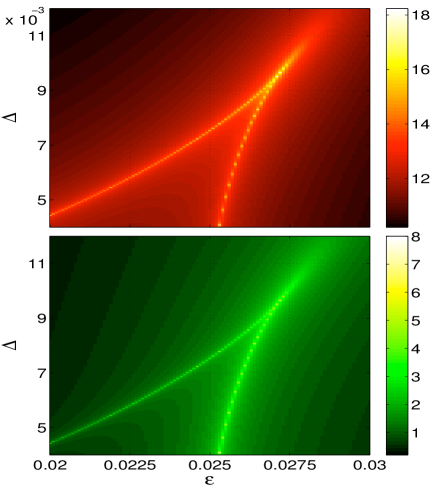
Figure 3: Identifying the triple exceptional point EP3. The upper panel shows the 2-D function $F(\Delta,\epsilon,\Gamma)$ presented in the text. The highest point corresponds to the triple-EP point EP3. The lower panel shows the sum of the absolute values of the amplitudes, which were calculated by the regular harmonic inversion method.

An efficient algorithm to identify the EP3 is demonstrated based on a two-dimensional search in the parameter space of $\Delta$ and $\epsilon$. This procedure enables the experimentalists to identify accurately the laser parameters for which the EP3 is obtained. We use the maximum of the function Eq. (19) as the objective leading to EP3.

Evaluating the function at each desired point in the parameter space include the following steps:

1. Time series: Obtain a time series of the polarization by performing the experiment or the numerical simulation.

2. Frequencies: Calculate the frequencies from the time series by harmonic inversion.

3. Function evaluation: Evaluate the function $F(\Delta,\epsilon,\Gamma)$ from the calculated frequencies.

Standard search methods can stagnate due to the high values at the EP2 curve. Another difficulty is the cusp behaviour of the EP2 curve close to the EP3. To overcome these diffculties we implemented a "climbing the valley" procedure: Staying on the valley of the local minima ensures the search overcomes the stagnation due to the EP2 curve. The procedure follows:

1. Preliminary step - initial point:

   1. Locate points inside the triangle-like EP curve (Cf. Fig. 4). The inner area of the curve is characterized by real-only eigenvalues.

   2. Perform a 1-D search to find a minimum on a straight line.

2. Valley ascend: Each iteration ascends up the valley to a point with higher value of the function $F$. This is done by finding a minimum on the circular arc that is centred at the current point, enclosed by two radii. The angles of these radii can be predefined or defined on each iteration. We perform the following steps:

   1. Determining the angular range. Predefined or from the previous iterations.

   2. Determining the radius. The radius is the distance from the current point to nearest point on the EP2 curve that is in the angular range.

   3. Finding the next point. Performing a 1-D search on the circular arc that is defined by the angular range and the radius (Cf. blue arc in Fig. 4). The point for the next iteration is the point on the arc with the minimal value of $F$ (Cf. end of green line in Fig. 4).

   These steps converge to the desired EP3 point. Figure 4 demonstrates the progress in the "valley ascend" method with a few iterations.

The Valley ascend method presented above is a generic method, and can be used also for searching higher order degeneracies in other systems. For the Bloch equation case, where the generating matrix, Eq. (18), is a $3\times 3$ matrix, the EP3 is the point where the characteristic polynomial

$$P_{{}_{\Delta,\epsilon,\Gamma}}(\omega)=(\omega-\omega_{1})(\omega-\omega_{2})(\omega-\omega_{3})$$ (20)

has roots with multiplicity of 3. Therefore we can use the special properties of the cubic equation and perform a regular root search. We define $r$, $s$ and $t$ as the coefficient of the polynomial $P_{{}_{\Delta,\epsilon,\Gamma}}(\omega)$ defined in Eq. (20):

$$(\omega-\omega_{1})(\omega-\omega_{2})(\omega-\omega_{3})=\omega^{3}+r\omega^{2}+s\omega+t.$$ (21)

We define the functions

$$\begin{array}[]{rcl}p(\Delta,\epsilon,\Gamma)&=&s-\frac{1}{3}r^{2}\\ q(\Delta,\epsilon,\Gamma)&=&\frac{2}{27}r^{3}-\frac{1}{3}rs+t,\end{array}$$ (22)

and perform a 2D conventional root search. The point in the parameter space where these two functions vanish is point where the three eigenvalues are degenerate. We have applied this method using standard method of 2D root search obtaining high accurate values of the $EP3$.

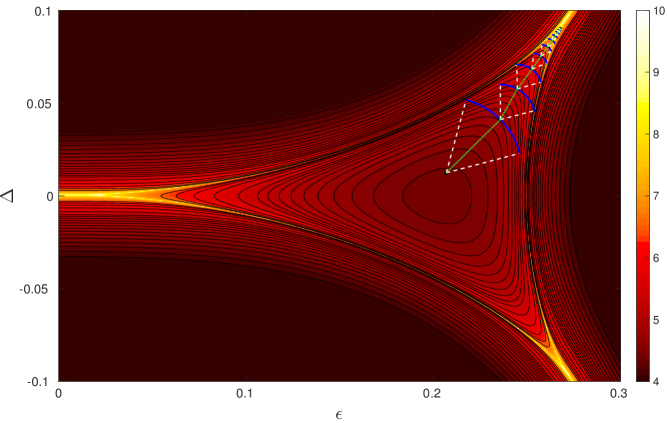
Figure 4: A sketch of the iterations progress in the "valley ascend" method. The collors on the background and the black contour lines represent the function $F(\Delta,\epsilon,\Gamma)$ of Eq. (19). In each iteration we plotted with blue line the circular arc on which we searched for the minimum. The black asterisks show these minima, which form the curve, plotted with a dashed light green line, that "climbs" in the valley of the objective function.

4.3.2 Physical parameter estimation from the value at the exceptional point

For the two-level-system the system parameters are the frequency $\omega_{s}$ associated with the energy gap, the general decay rate $\Gamma$ and the dipole strength $\mu$. The external experimentally controlled parameters are the driving frequency $\nu$ and the power amplitude $\cal E$. The parameters of Eq. (18) can be related with $\epsilon=\mu{\cal E}$ and $\Delta=\omega_{s}-\nu$. One would like to estimate the system parameters from experiments. After locating accurately the EP, we can determine the parameters by inverting the relations between the eigenvalues and the system parameters.

To obtain high accuracy, we used the identification the triple-degeneracy point EP3 presented above, so both parameters - $\Delta$ and $\epsilon$ - are located accurately. The accurate location of $\Delta$ and $\epsilon$ makes the parameter estimation very robust to uncertainties in the location of the exceptional points. This is a consequence of the special non analytic character close to the EP3 (Cf. D). Therefore, the system parameters $\Gamma$, $\omega_{s}$ and $\mu$ can be determined to a high degree of accuracy at this point. From the eigenvalues of the matrix M in Eq. (18) we get $\Gamma=\frac{i}{2}\left(\omega_{1}+\omega_{2}+\omega_{3}\right)$. To obtain $\epsilon$ and $\Delta$ one has to invert non-linear relations (see C). At the EP3, the inversion becomes: $\textstyle\omega_{s}=\nu+\sqrt{1/108}\,\Gamma$, $\mu=\sqrt{8/108}\,\Gamma/{\cal E}$.

4.3.3 Noise sensitivity

Parameters estimation naturally raises the issue of sensitivity to noisy experimental data. The noise sensitivity will be determined by the method of harmonic inversion. If the sampling periods have high accuracy then the time series can be shown to have an underlying Hamiltonian generator. This is the basis for linear methods, such as the filter diagonalization (FD) [49, 50]. The noise in these methods results in normally distributed underlying matrices, and the model displays monotonous behaviour with respect to the noise. This was verified analytically and by means of simulations In Ref. [60]. As a result sufficient averaging will eliminate the noise. Practical implementations require further analysis with evidence of nonlinear effects of noise. For example, Mandelshtam et. al. analysed the noise-sensitivity of the FD in the context of NMR experiments [61, 62] and Fourier transform mass spectrometry [63]. For some other methods, a noise reduction technique was proposed in Ref. [51].

5 Discussion

Bloch’s equation has become the template for the dynamics of open quantum systems. Such systems typically decohere with a dynamical signature of decaying oscillatory motion. It is therefore surprising that the existence of non hermitian degeneracies has been overlooked. Our finding of an intricate manifold of double degeneracies EP2 and triple degeneracies EP3 in the elementary TLS template suggests that any quantum dynamics described by the L-GKS generator [25, 26] will exhibit a manifold of exceptional points.

Non hermitian degeneracies of the EP have a subtle influence on the dynamics. The hallmark of EP dynamics is a polynomial component in the decay leading to non-Lorentzian lineshapes. We suggest an experimental procedure to identify the EP in Bloch systems, using harmonic inversion of the polarization time series. The sensitivity of harmonic inversion in the neighbourhood of an EP enables us to accurately locate the EP, and therefore allows us to determine the system parameters: the energy gap $\omega_{s}$, the dipole transition moment $\mu$, and the decoherence rate $\Gamma$.

This study is only the first step in establishing parameter estimation via exceptional points. A generalization to larger Liouville spaces is under study for atomic spectroscopy. Under the influence of driving fields and due to spontaneous emission, atoms and ions can have a structure of N-level system with relaxation. In these systems we expect non-hermitian degeneracy of high order. The structure of the exceptional points in these systems can be used for estimating the energy differences, the lifetimes, and branching ratios. work in this direction is in progress [64].

Many quantum systems are open and their dynamics has dissipative nature, which is described well by the L-GKS equation. Therefore we expect to find exceptional points in many quantum systems. Under the appropriate circumstances these EPs can be used for accurate parameter estimation.

Aknowledgements

We thank Ido Schaefer, Amikam Levy, and Raam Uzdin for fruitful discussions. We thank Jacob Fuchs and Jörg Main for assisting with the extended harmonic inversion method. We thank the referee for proposing the root search for the EP3. Work supported by the Israel Science Foundation Grants No. 2244/14 and No. 298/11 and by I-Core: the Israeli Excellence Center “Circle of Light”.

Appendix A Bloch equations

The Bloch equation describes the dynamics of the three components of the nuclear spin, $S_{x}$, $S_{y}$, and $S_{z}$, under the influence of an external magnetic field $\vec{H}$. The equations as appear in Bloch’s original paper ([1], Eq. 38) are

$$\begin{array}[]{rcl}\dot{S_{x}}&=&\gamma\left(S_{y}H_{z}-S_{z}H_{y}\right)-\frac{1}{T_{2}}S_{x}\\ \dot{S_{y}}&=&\gamma\left(S_{z}H_{x}-S_{x}H_{z}\right)-\frac{1}{T_{2}}S_{y}\\ \dot{S_{z}}&=&\gamma\left(S_{x}H_{y}-S_{y}H_{x}\right)-\frac{1}{T_{1}}\left(S_{z}-S_{z}^{0}\right).\end{array}$$ (26)

$T_{1}$ and $T_{2}$ are two relaxation parameters (the pure dephasing rate $\frac{1}{T_{2}^{*}}$ is related by $\frac{1}{T_{2}}=\frac{1}{2T_{1}}+\frac{1}{T_{2}^{*}}$), $\gamma$ is the gyromagnetic ratio, and $S_{z}^{0}$ is the equilibrium value of $S_{z}$ under the influence of constant external magnetic field $H_{z}=H_{0}$. These equations can be recast in a matrix-vector notation:

$$\frac{d}{dt}\left(\begin{array}[]{c}S_{x}\\ S_{y}\\ S_{z}\end{array}\right)=\left(\begin{array}[]{ccc}-\frac{1}{T_{2}}&\gamma H_{z}&-\gamma H_{y}\\ -\gamma H_{z}&-\frac{1}{T_{2}}&\gamma H_{x}\\ \gamma H_{y}&-\gamma H_{x}&-\frac{1}{T_{1}}\end{array}\right)\left(\begin{array}[]{c}S_{x}\\ S_{y}\\ S_{z}\end{array}\right)+\left(\begin{array}[]{c}0\\ 0\\ \frac{1}{T_{1}}S_{z}^{0}\end{array}\right).$$ (39)

For an external field $\vec{H}$ with the components $H_{x}=H_{1}\cos\omega t$ , $H_{y}=-H_{1}\sin\omega t$, $H_{z}=H_{0}$, we define the rotating frame:

$$\begin{array}[]{rcl}S_{x}&=&\phantom{-}\tilde{S_{x}}\cos\omega t-\tilde{S_{y}}\sin\omega t\\ S_{y}&=&-\tilde{S_{x}}\sin\omega t-\tilde{S_{y}}\cos\omega t\\ .\end{array}$$ (43)

With the notations $\epsilon=\gamma H_{1}$ and $\Delta=\gamma H_{0}-\omega$ we have (see also [4]):

$$\frac{d}{dt}\left(\begin{array}[]{c}\tilde{S}_{x}\\ \tilde{S}_{y}\\ S_{z}\end{array}\right)=\left(\begin{array}[]{ccc}-\frac{1}{T_{2}}&\Delta&0\\ -\Delta&-\frac{1}{T_{2}}&\epsilon\\ 0&-\epsilon&-\frac{1}{T_{1}}\end{array}\right)\left(\begin{array}[]{c}\tilde{S}_{x}\\ \tilde{S}_{y}\\ S_{z}\end{array}\right)+\left(\begin{array}[]{c}0\\ 0\\ \frac{1}{T_{1}}S_{z}^{0}\end{array}\right).$$ (56)

These equations also describe, in the dipole approximation, a two-level atom in external electromagnetic field. In this case, the system parameters are the the unperturbed frequency of the system $\omega_{s}$, and the dipole strength $\mu$. The external experimentally controlled parameters are the driving frequency $\nu$ and the power amplitude $\cal E$. The parameters of Eq. (56) are related with $\epsilon=\mu{\cal E}$ and $\Delta=\omega_{s}-\nu$. In the absence of dissipation the eigenvalues of the matrix are pure imaginary, and the dynamics is a free precession of the polarization vector characterized by the Rabi frequency: $\Omega=\sqrt{\epsilon^{2}+\Delta^{2}}$. When dissipation is present the eigenvalues of the homogeneous part of Eq. (56) become complex, reflecting a decaying oscillation dynamics leading asymptotically to a steady state.

Appendix B Derivation of the Bloch equation from the L-GKS equation

In the Heisenberg representation the L-GKS generator becomes:

$$\frac{d}{dt}{\bm{\mathrm{\hat{X}}}}~{}=~{}\frac{\partial{\bm{\mathrm{\hat{X}}}}}{\partial t}+i\left[\hat{\bm{\text{H}}},{\bm{\mathrm{\hat{X}}}}\right]+\sum_{k}\left(\hat{\bm{\text{V}}}_{k}^{\dagger}{\bm{\mathrm{\hat{X}}}}\hat{\bm{\text{V}}}_{k}-\frac{1}{2}\left\{\hat{\bm{\text{V}}}_{k}^{\dagger}\hat{\bm{\text{V}}}_{k},{\bm{\mathrm{\hat{X}}}}\right\}\right).$$ (57)

where ${\bm{\mathrm{\hat{X}}}}$ is an arbitrary operator. The Hamiltonian ${\bm{\mathrm{\hat{H}}}}$ is hermitian and ${\bm{\mathrm{\hat{V}}}}$ is defined to operate in the Hilbert space of the system. The curly brackets denote an anti commutator. The set of operators $\{{\bm{\mathrm{\hat{X}}}}\}$ supports a Hilbert space construction, with the scalar product defined as: $\left({\bm{\mathrm{\hat{X}}}}_{1},{\bm{\mathrm{\hat{X}}}}_{2}\right)\equiv tr\left\{{\bm{\mathrm{\hat{X}}}}_{1}^{\dagger}{\bm{\mathrm{\hat{X}}}}_{2}\right\}$.

For two-level system, the effective rotating-frame Hamiltonian under a driving field with detuning $\Delta$ and driving frequency $\epsilon$ is:

$${\bm{\mathrm{\hat{H}}}}=\Delta{\bm{\mathrm{\hat{S}}}}_{z}+\epsilon\bm{\mathrm{\tilde{S}}}_{x}$$ (58)

The two-level-system L-GKS equation for an operator ${\bm{\mathrm{\hat{X}}}}$ with relaxation and pure dephasing becomes

$$\begin{array}[]{rcl}\frac{d}{dt}{\bm{\mathrm{\hat{X}}}}&=&i\;[{\bm{\mathrm{\hat{H}}}},{\bm{\mathrm{\hat{X}}}}]\\ &&+\,\kappa_{-}\left({\bm{\mathrm{\hat{S}}}}_{+}{\bm{\mathrm{\hat{X}}}}{\bm{\mathrm{\hat{S}}}}_{-}-\frac{1}{2}\{{\bm{\mathrm{\hat{S}}}}_{+}{\bm{\mathrm{\hat{S}}}}_{-},{\bm{\mathrm{\hat{X}}}}\}\right)\\ &&+\,\kappa_{+}\left({\bm{\mathrm{\hat{S}}}}_{-}{\bm{\mathrm{\hat{X}}}}{\bm{\mathrm{\hat{S}}}}_{+}-\frac{1}{2}\{{\bm{\mathrm{\hat{S}}}}_{-}{\bm{\mathrm{\hat{S}}}}_{+},{\bm{\mathrm{\hat{X}}}}\}\right)\\ &&-\,\gamma\;[{\bm{\mathrm{\hat{S}}}}_{z},[{\bm{\mathrm{\hat{S}}}}_{z},{\bm{\mathrm{\hat{X}}}}]]\end{array}$$ (59)

where $\kappa_{\pm}$ are kinetic coefficients, $\kappa_{+}/\kappa_{-}=\exp(-\hbar\omega/k_{B}T)$, and $\gamma$ is the pure dephasing rate [2, 65].

To rephrase the equation in a matrix-vector notation, We use the polarization operators and the identity matrix to form the vector of basis operators: $\vec{S}^{\prime}=\left(\bm{\mathrm{\tilde{S}}}_{x},\bm{\mathrm{\tilde{S}}}_{y},{\bm{\mathrm{\hat{S}}}}_{z},{\bm{\mathrm{\hat{I}}}}\right)^{T}$. Then Eq. (59) can be written as $\dot{\vec{S}^{\prime}}=M^{\prime}\vec{S}^{\prime}$, with an appropriate $4\times 4$ matrix $M^{\prime}$. We can reduce the dimensions by writing an inhomogeneous equation for the 3-component vector $\vec{S}=\left(\bm{\mathrm{\tilde{S}}}_{x},\bm{\mathrm{\tilde{S}}}_{y},{\bm{\mathrm{\hat{S}}}}_{z}\right)^{T}$:

$$\dot{\vec{S}}=\left(M-\gamma I\right)\left(\vec{S}-\vec{S}_{eq}\right),$$ (60)

with $\Gamma=\kappa_{-}+\kappa_{+}-\gamma$, $I$ as the $3\times 3$ identity matrix, $\vec{S}_{eq}$ that fulfills $(\gamma I-M)\vec{S}_{eq}=\left(0,0,(\kappa_{+}-\kappa_{-}){\bm{\mathrm{\hat{I}}}}\right)^{T}$ and the matrix:

$$\text{M}=\left(\begin{array}[]{ccc}-\frac{\Gamma}{2}&\Delta&0\\ -\Delta&-\frac{\Gamma}{2}&\epsilon\\ 0&-\epsilon&\text{-$\Gamma$}\end{array}\right).$$ (61)

Eq. (60) can be merged with the Bloch’s equation (56) where $\frac{1}{T_{1}}=\kappa_{+}+\kappa_{-}$ and $\frac{1}{T_{2}}=\gamma+\frac{1}{2}(\kappa_{+}+\kappa_{-})$.

The general solution for this equation is:

$$\vec{S}(t)=e^{-\gamma t}e^{\text{M}t}(\vec{S}_{0}-\vec{S}_{eq})+\vec{S}_{eq},$$ (62)

with $\vec{S}_{0}=\vec{S}(0)$.

The master equation Eq. (59) is a common form for TLS found in the literature [66, 67, 7]. Eq. (61) which determines the EP interpolates between two extreme cases. The first is associated with spontaneous emission, then $\Gamma=\kappa_{-}$. The second is a hot singular bath dominated by pure dephasing, then $\Gamma=-\gamma$.

Appendix C Eigenvalues of the matrix M

The task is to find the eigenvalues of the generator matrix (18).

We first define the variables:

$$\begin{array}[]{rcr}Y&=&12\Delta^{2}+12\epsilon^{2}-\text{$\Gamma$}^{2}\\ X&=&-36\Delta^{2}+18\epsilon^{2}-\Gamma^{2}\end{array}$$ (63)

We also define:

$$\begin{array}[]{rcl}W&=&\sqrt{\Gamma^{2}X^{2}+Y^{3}}\\ &=&\left(\Gamma^{4}\Delta^{2}+16\left(\Delta^{2}+\epsilon^{2}\right)^{3}+\Gamma^{2}\left(8\Delta^{4}-20\Delta^{2}\epsilon^{2}-\epsilon^{4}\right)\right)^{1/2}.\end{array}$$ (64)

With these definitions the eigenvalues of Eq. (18) become:

$$\begin{array}[]{ccc}m_{1}&=&-\frac{2}{3}\Gamma+\frac{1}{6}\left(\left(W+\Gamma X\right)^{1/3}-\frac{Y}{\left(W+\Gamma X\right)^{1/3}}\right)\\ m_{2}&=&-\frac{2}{3}\Gamma+\frac{1}{6}\left(e^{i\frac{2}{3}\pi}\left(W+\Gamma X\right)^{1/3}+e^{i\frac{1}{3}\pi}\frac{Y}{\left(W+\Gamma X\right)^{1/3}}\right)\\ m_{3}&=&-\frac{2}{3}\Gamma+\frac{1}{6}\left(e^{-i\frac{2}{3}\pi}\left(W+\Gamma X\right)^{1/3}+e^{-i\frac{1}{3}\pi}\frac{Y}{\left(W+\Gamma X\right)^{1/3}}\right).\end{array}$$ (65)

For real $W$ (i.e. for $\Gamma^{2}X^{2}+Y^{3}\geq 0$) all eigenvalues are real. For $\Gamma^{2}X^{2}+Y^{3}<0$, $W$ is complex, and two of the eigenvalues are complex (complex conjugate to each other).

Non-hermitian degeneracies of the eigenvalues occur when $W$ vanishes. In such cases the second and third eigenvalues are degenerated, leading to EP2. A third order exceptional point, EP3, occurs for $X=Y=0$. This happens when $\Delta=\pm\sqrt{1/108}\,\Gamma$, $\epsilon=\sqrt{8/108}\,\Gamma$. These triple-degeneracies EP3 occur twice, and have a cusp-like behaviour, emerging from the EP2-curves, identifiable as an elliptic umbilic catastrophe [56]. This topology is also consistent with the analysis of non hermitian degeneracies of a two-parameters family of $3\times 3$ matrices, done by Mailybaev [57]. In very strong driving fields the matrix $M$ will loose symmetry [58, 59] maintaining the cusps but skewing the topology.

Appendix D non analytic character close to the EP3

There is a special non analytic character close to the EP3: When $\nu\to\nu^{EP3}$ and ${\cal E}\to{\cal E}^{EP3}$ then the three frequencies obtained by the standard harmonic inversion coalesce, leading to a branch point (Cf. Chapter 9 in Ref. [29]):

$$\omega_{k=1,2,3}=\omega_{1}^{(2)}+e^{i\frac{2\pi}{3}}\left[\alpha_{k}(\nu-\nu^{EP3})+\beta_{k}({\cal E}-{\cal E}^{EP3})\right]^{\frac{1}{3}}$$ (66)

where $\alpha_{k}$ and $\beta_{k}$ are parameters. At the EP3, i.e. for $\nu\to\nu^{EP3}$ and ${\cal E}\to{\cal E}^{EP3}$, we get $\partial\omega_{k}/\partial\nu\to\infty$ and $\partial\omega_{k}/\partial{\cal E}\to\infty$, leading to $\partial\Gamma/\partial\nu\to\infty$ and $\partial\Gamma/\partial{\cal E}\to\infty$.

Bibliography

Bibliography

- [1] Felix Bloch. Nuclear induction. Physical review, 70(7-8):460, 1946.
- [2] GS Agarwal. Master-equation approach to spontaneous emission. Physical Review A, 2(5):2038, 1970.
- [3] Claude Cohen-Tannoudji, Jacques Dupont-Roc, and Gilbert Grynberg. Atom-Photon Interactions: Basic Process and Appilcations, chapter Optical Bloch Equations, pages 353–405. Wiley-VCH Verlag GmbH, Weinheim, Germany, 1998.
- [4] Ralph G. DeVoe and Richard G. Brewer. Experimental test of the optical bloch equations for solids. Phys. Rev. Lett., 50:1269–1272, Apr 1983.
- [5] Seth Lloyd. Almost any quantum logic gate is universal. Physical Review Letters, 75(2):346, 1995.
- [6] A Zrenner, E Beham, S Stufler, F Findeis, M Bichler, and G Abstreiter. Coherent properties of a two-level system based on a quantum-dot photodiode. Nature, 418(6898):612–614, 2002.
- [7] Søren Gammelmark and Klaus Mølmer. Fisher information and the quantum cramér-rao sensitivity limit of continuous measurements. Physical Review Letters, 112(17):170401, 2014.
- [8] John Clarke and Frank K Wilhelm. Superconducting quantum bits. Nature, 453(7198):1031–1042, 2008.
- [9] Thaddeus D Ladd, Fedor Jelezko, Raymond Laflamme, Yasunobu Nakamura, Christopher Monroe, and Jeremy L OBrien. Quantum computers. Nature, 464(7285):45–53, 2010.
- [10] E Lisi, A Marrone, and D Montanino. Probing possible decoherence effects in atmospheric neutrino oscillations. Physical Review Letters, 85(6):1166, 2000.
- [11] J. Six. Test of the non separability of the system. Physics Letters B, 114(2):200–202, 1982.
- [12] F. Selleri. Einstein locality and the 946-1 0 system. Lett. Neovo Cim., 36:521, 1983.
- [13] Paolo Privitera and Franco Selleri. Quantum mechanics versus local realism for neutral kaon pairs. Physics Letters B, 296(1):261–272, 1992.
- [14] Amitava Datta and Dipankar Home. Quantum non-separability versus local realism: A new test using the b0b0 system. Physics Letters A, 119(1):3–6, 1986.
- [15] R. Lo Franco, A. D’Arrigo, G. Falci, G. Compagno, and E. Paladino. Preserving entanglement and nonlocality in solid-state qubits by dynamical decoupling. Phys. Rev. B, 90:054304, Aug 2014.
- [16] John S Bell et al. Speakable and unspeakable in quantum mechanics. Speakable and Unspeakable in Quantum Mechanics, by JS Bell, Introduction by Alain Aspect, Cambridge, UK: Cambridge University Press, 2004, 1, 2004.
- [17] L Essen and JVL Parry. An atomic standard of frequency and time interval: A cæsium resonator. Nature, 176:280–282, 1955.
- [18] Vittorio Giovannetti, Seth Lloyd, and Lorenzo Maccone. Quantum-enhanced measurements: beating the standard quantum limit. Science, 306(5700):1330–1336, 2004.
- [19] S. F. Huelga, C. Macchiavello, T. Pellizzari, A. K. Ekert, M. B. Plenio, and J. I. Cirac. Improvement of frequency standards with quantum entanglement. Phys. Rev. Lett., 79:3865–3868, Nov 1997.
- [20] G. Arrad, Y. Vinkler, D. Aharonov, and A. Retzker. Increasing sensing resolution with error correction. Phys. Rev. Lett., 112:150801, Apr 2014.
- [21] Roald K Wangsness and Felix Bloch. The dynamical theory of nuclear induction. Physical Review, 89(4):728, 1953.
- [22] Felix Bloch. Generalized theory of relaxation. Physical Review, 105(4):1206, 1957.
- [23] E Brian Davies. Markovian master equations. Communications in mathematical Physics, 39(2):91–110, 1974.
- [24] Karl Kraus. States, effects and operations. Springer, 1983.
- [25] Goran Lindblad. On the generators of quantum dynamical semigroups. Communications in Mathematical Physics, 48(2):119–130, 1976.
- [26] Vittorio Gorini, Andrzej Kossakowski, and Ennackal Chandy George Sudarshan. Completely positive dynamical semigroups of n-level systems. Journal of Mathematical Physics, 17(5):821–825, 1976.
- [27] Heinz-Peter Breuer and Francesco Petruccione. The theory of open quantum systems. Oxford university press, 2002.
- [28] Shaul Mukamel. Principles of nonlinear optical spectroscopy. Number 6. Oxford University Press, 1999.
- [29] Nimrod Moiseyev. Non-Hermitian quantum mechanics. Cambridge University Press Cambridge, 2011.
- [30] Robert Alicki and Karl Lendi. Quantum Dynamical Semigroups and Applications, volume 717 of Lecture Notes in Physics. Springer Berlin Heidelberg, 2007.
- [31] U. Fano. Effects of configuration interaction on intensities and phase shifts. Phys. Rev., 124:1866–1878, Dec 1961.
- [32] Ingrid Rotter. A non-hermitian hamilton operator and the physics of open quantum systems. Journal of Physics A: Mathematical and Theoretical, 42(15):153001, 2009.
- [33] MV Berry. Physics of nonhermitian degeneracies. Czechoslovak journal of physics, 54(10):1039–1047, 2004.
- [34] Raam Uzdin and Nimrod Moiseyev. Scattering from a waveguide by cycling a non-hermitian degeneracy. Physical Review A, 85(3):031804, 2012.
- [35] O Latinne, NJ Kylstra, M Dörr, J Purvis, M Terao-Dunseath, CJ Joachain, PG Burke, and CJ Noble. Laser-induced degeneracies involving autoionizing states in complex atoms. Physical review letters, 74(1):46, 1995.
- [36] Holger Cartarius, Jörg Main, and Günter Wunner. Exceptional points in atomic spectra. Physical review letters, 99(17):173003, 2007.
- [37] Raam Uzdin, Emanuele G Dalla Torre, Ronnie Kosloff, and Nimrod Moiseyev. Effects of an exceptional point on the dynamics of a single particle in a time-dependent harmonic trap. Physical Review A, 88(2):022505, 2013.
- [38] Nimrod Moiseyev. Sudden transition from a stable to an unstable harmonic trap as the adiabatic potential parameter is varied in a time-periodic harmonic trap. Physical Review A, 88(3):034502, 2013.
- [39] A I Magunov, I Rotter, and S I Strakhova. Laser-induced resonance trapping in atoms. Journal of Physics B: Atomic, Molecular and Optical Physics, 32(7):1669, 1999.
- [40] A I Magunov, I Rotter, and S I Strakhova. Laser-induced continuum structures and double poles of the s -matrix. Journal of Physics B: Atomic, Molecular and Optical Physics, 34(1):29, 2001.
- [41] Edvardas Narevicius and Nimrod Moiseyev. Trapping of an electron due to molecular vibrations. Physical review letters, 84(8):1681, 2000.
- [42] J Rubinstein, P Sternberg, and Q Ma. Bifurcation diagram and pattern formation of phase slip centers in superconducting wires driven with electric currents. Physical review letters, 99(16):167003, 2007.
- [43] Pavel Cejnar, Stefan Heinze, and Michal Macek. Coulomb analogy for non-hermitian degeneracies near quantum phase transitions. Physical review letters, 99(10):100601, 2007.
- [44] C Dembowski, H-D Gräf, HL Harney, A Heine, WD Heiss, H Rehfeld, and A Richter. Experimental observation of the topological structure of exceptional points. Physical review letters, 86(5):787, 2001.
- [45] Shachar Klaiman, Uwe Günther, and Nimrod Moiseyev. Visualization of branch points in p t-symmetric waveguides. Physical review letters, 101(8):080402, 2008.
- [46] Markus Müller and Ingrid Rotter. Exceptional points in open quantum systems. Journal of Physics A: Mathematical and Theoretical, 41(24):244018, 2008.
- [47] Markus Müller and Ingrid Rotter. Phase lapses in open quantum systems and the non-hermitian hamilton operator. Phys. Rev. A, 80:042705, Oct 2009.
- [48] Jan Wiersig. Enhancing the sensitivity of frequency and energy splitting detection by using exceptional points: Application to microcavity sensors for single-particle detection. Phys. Rev. Lett., 112:203901, May 2014.
- [49] Michael R. Wall and Daniel Neuhauser. Extraction, through filter-diagonalization, of general quantum eigenvalues or classical normal mode frequencies from a small number of residues or a short-time segment of a signal. i. theory and application to a quantum-dynamics model. The Journal of Chemical Physics, 102(20):8011–8022, 1995.
- [50] Vladimir A Mandelshtam. Fdm: the filter diagonalization method for data processing in nmr experiments. Progress in Nuclear Magnetic Resonance Spectroscopy, 38(2):159–196, 2001.
- [51] Dž. Belkić, P. A. Dando, J. Main, and H. S. Taylor. Three novel high-resolution nonlinear methods for fast signal processing. The Journal of Chemical Physics, 113(16):6542–6556, 2000.
- [52] Jacob Fuchs, Jörg Main, Holger Cartarius, and Günter Wunner. Harmonic inversion analysis of exceptional points in resonance spectra. Journal of Physics A: Mathematical and Theoretical, 47(12):125304, 2014.
- [53] Heung-Ryoul Noh and Wonho Jhe. Analytic solutions of the optical bloch equations. Optics Communications, 283(11):2353 – 2355, 2010.
- [54] Alexander Moroz. On unorthodox solutions of the bloch equations. arXiv preprint arXiv:1208.5736, 2012.
- [55] Heung-Ryoul Noh. Optical bloch equations for a two-level atom revisited: Analytical solutions. Journal of the Physical Society of Japan, 84(9):094402, 2015.
- [56] Michael V Berry, JF Nye, and FJ Wright. The elliptic umbilic diffraction catastrophe. Philosophical Transactions for the Royal Society of London. Series A, Mathematical and Physical Sciences, pages 453–484, 1979.
- [57] Alexei A. Mailybaev. Computation of multiple eigenvalues and generalized eigenvectors for matrices dependent on parameters. Numerical Linear Algebra with Applications, 13(5):419–436, 2006.
- [58] Eitan Geva, Ronnie Kosloff, and JL Skinner. On the relaxation of a two-level system driven by a strong electromagnetic field. The Journal of chemical physics, 102(21):8541–8561, 1995.
- [59] Krzysztof Szczygielski, David Gelbwaser-Klimovsky, and Robert Alicki. Markovian master equation and thermodynamics of a two-level system in a strong laser field. Physical Review E, 87(1):012120, 2013.
- [60] Uroš Benko and Đani Juričić. Frequency analysis of noisy short-time stationary signals using filter-diagonalization. Signal Processing, 88(7):1733 – 1746, 2008.
- [61] Haitao Hu, Que N. Van, Vladimir A. Mandelshtam, and A.J. Shaka. Reference deconvolution, phase correction, and line listing of NMR spectra by the 1d filter diagonalization method. Journal of Magnetic Resonance, 134(1):76 – 87, 1998.
- [62] Hasan Celik, A.J. Shaka, and V.A. Mandelshtam. Sensitivity analysis of solutions of the harmonic inversion problem: Are all data points created equal? Journal of Magnetic Resonance, 206(1):120 – 126, 2010.
- [63] Beau R. Martini, Konstantin Aizikov, and Vladimir A. Mandelshtam. The filter diagonalization method and its assessment for Fourier transform mass spectrometry. International Journal of Mass Spectrometry, 373(0):1 – 14, 2014.
- [64] Morag Am-Shallem, Ronnie Kosloff, and Nimrod Moiseyev. Parameter estimation in atomic spectroscopy using exceptional points. arXiv preprint arXiv:1511.07205, 2015.
- [65] Gérard G Emch and Joseph C Varilly. On the standard form of the bloch equation. Letters in Mathematical Physics, 3(2):113–116, 1979.
- [66] GL Fogli, E Lisi, A Marrone, D Montanino, and A Palazzo. Probing nonstandard decoherence effects with solar and kamland neutrinos. Physical Review D, 76(3):033006, 2007.
- [67] S Gammelmark, K Mølmer, W Alt, T Kampschulte, and D Meschede. Hidden markov model of atomic quantum jump dynamics in an optically probed cavity. Physical Review A, 89(4):043839, 2014.