Effective field theory of Bose–Einstein condensation of $\alpha$ clusters and Nambu–Goldstone–Higgs states in ¹²C

Abstract

An effective field theory of $\alpha$ cluster condensation is formulated as a spontaneously broken symmetry in quantum field theory to understand the raison d’être and nature of the Hoyle and $\alpha$ cluster states in ¹²C. The Nambu–Goldstone and Higgs mode operators in infinite systems are replaced with a pair of canonical operators whose Hamiltonian gives rise to discrete energy states in addition to the Bogoliubov–de Gennes excited states. The calculations reproduce well the experimental spectrum of the $\alpha$ cluster states. The existence of the Nambu–Goldstone–Higgs states is demonstrated and crucial. The $\gamma$ decay transitions are also obtained.

I Introduction

Alpha cluster condensation in nuclei has attracted much attention since the observation of Bose–Einstein condensation (BEC) of trapped cold atoms Cornel2002 . In ¹²C, the three-$\alpha$ structure was most thoroughly investigated by Uegaki et al. Uegaki1977 , who showed that the $0_{2}^{+}$ state at an excitation energy $E_{x}$ of 7.654 MeV, the Hoyle state, which is crucial for nucleosynthesis, the evolution of stars, and the emergence of life, has a dilute structure in a new “$\alpha$-boson gas phase” and clarified the systematic existence of a “new phase” of three $\alpha$ clusters above the $\alpha$ threshold. The Hoyle state has been extensively studied theoretically Tohsaki2001 ; Yamada2004 ; Ohkubo2004 ; Yamada2005 ; Kurokawa2005 ; Kurokawa2007 ; Kanada2007 ; Chernykh2007 ; Roth2011 ; Epelbaum2012 ; Dreyfuss2013 and experimentally Freer2009 ; Itoh2011 ; Zimmerman2011 ; Zimmerman2013 ; Itoh2013 ; Freer2014 ; Freer2011 ; Ogloblin2014 , and has been considered widely as an $\alpha$ cluster condensate. It has a gas-like structure with a dilute matter distribution of three-$\alpha$ clusters, 70% of which are in the $0$s state Yamada2005 . However, no firm evidence of BEC, such as superfluidity, has been found.

In ¹²C, all the excited states except the $2_{1}^{+}$ state at 4.44 MeV appear above the $\alpha$ particle threshold (7.367 MeV). Recently, $\alpha$ cluster states above the Hoyle state, which are also candidates for an $\alpha$ cluster condensate, that is, the $0_{3}^{+}$ state at 9.04 MeV, $0_{4}^{+}$ state at 10.56 MeV, $2_{2}^{+}$ state ($\sim$9.75 MeV) Itoh2011 ; Itoh2013 ; Freer2009 ; Zimmerman2011 ; Zimmerman2013 , and $4_{1}^{+}$ state ($\sim$13.3 MeV) Freer2011 ; Ogloblin2014 have been observed. To date, studies using $\alpha$ cluster models Yamada2005 ; Kurokawa2005 ; Kurokawa2007 and ab initio calculations Kanada2007 ; Chernykh2007 ; Roth2011 ; Epelbaum2012 ; Dreyfuss2013 explain the Hoyle state and the excited gas-like states as collective states of $\alpha$ clusters or nucleons in configuration space. Collective motions arise owing mostly to spontaneously broken symmetries (SBSs) in the configuration space, such as rotational and translational ones, or in the gauge space Ring1980 ; BalaizotRipka . The BEC of $\alpha$ clusters is a manifestation of the SBS of the global phase. It would be difficult from the standpoint of traditional $\alpha$ cluster models or ab initio calculations to conclude that BEC is truly realized, because it is not clear then what type of symmetry is broken for the Hoyle state and the $\alpha$ condensate states above it.

In the study of $\alpha$ cluster condensation, it is important to treat the SBS of the global phase on the basis of quantum field theory because of its unifying view and underlying principle. SBS is ubiquitous Watanabe2012 ; when it occurs, a Nambu–Goldstone (NG) mode (phason) appears according to the NG theorem Nambu1961 ; Goldstone1961 , and a Higgs (amplitude) mode (amplitudon) usually accompanies it. For example, in infinite superconducting systems, the NG mode Kadowaki1998 , which is eaten by the plasmon, and the Higgs mode Littlewood1981 ; Varma2001 have been observed. For systems with a finite particle number, both the NG and Higgs modes have been confirmed in superfluid nuclei as a pairing rotation and pairing vibration, respectively Broglia1973 . The observation of the Higgs boson in particle physics ATLAS2012 has stimulated a search for Higgs modes in other phenomena, including a recent experiment on Higgs mode excitation in a superconductor using a terahertz pulse Matsunaga2013 . It is intriguing to reveal the emergence of the NG and Higgs modes theoretically in an $\alpha$ cluster condensate and to observe them experimentally. Because the system is finite in size and particle number, they would manifest themselves not as particle excitations but as resonant states with discrete energy levels. From this viewpoint, Ref.Ohkubo2013 discussed a possible emergence of such states for an $\alpha$ cluster condensate in ¹²C and ¹⁶O qualitatively.

The purpose of this paper is to show for the first time that the dilute excited $\alpha$ cluster states, the Hoyle state and those above it, can be understood as new discrete states that follow naturally in the formulation of quantum field theory NTY , called the interacting zero mode formulation (IZMF in short), for BEC of $\alpha$ clusters in terms of the field equation, canonical commutation relations (CCRs), and global gauge invariance.

This paper is organized as follows. In Sect. II, the IZMF for BEC of trapped cold atoms is extended to BEC of $\alpha$ clusters. In Sect. III, we introduce a phenomenological model of $\alpha$ clusters, in which $\alpha$ particles are trapped by a harmonic potential and the $\alpha$-$\alpha$ interaction is described by a phenomenological Ali–Bodmer potential Ali1966 . Then, the strengths of the harmonic potential and the repulsive potential in the Ali–Bodmer potential are the key parameters in our analysis. We calculate the energy levels, adjusting the two parameters, and compare them with the observed $\alpha$ cluster states. The $\gamma$ decay transition probabilities are calculated in Sect. V. Sect. VI is devoted to the summary.

II Formulation of quantum field theory of Bose-Einstein condensation for $\alpha$ clusters

First, we clarify from quantum field theory for the $\alpha$ cluster condensate that the canonical operators NTY , which replace the NG and Higgs mode operators in infinite systems with SBS, emerge and that the spectrum of their quantum mechanical system is discrete.

We start with the following Hamiltonian for the $\alpha$ cluster system described by the field operator ${\hat{\psi}}$:

$$\hat{H}=\int\!d^{3}x\;\hat{\psi}^{\dagger}(x)\left(-\frac{\nabla^{2}}{2m}+V_{\mathrm{ex}}(\bm{x})-\mu\right)\hat{\psi}(x)$$

$$\,\,+\frac{1}{2}\int\!d^{3}x\,d^{3}x^{\prime}\;\hat{\psi}^{\dagger}(x)\hat{\psi}^{\dagger}(x^{\prime})U(|\bm{x}-\bm{x}^{\prime}|)\hat{\psi}(x^{\prime})\hat{\psi}(x)\,,$$ (1)

where $m$ and $\mu$ denote the mass of the $\alpha$ particle and the chemical potential, respectively. The external isotropic confinement potential $V_{\mathrm{ex}}(\bm{x})$ is introduced in a phenomenological manner that will be discussed later. The interaction potential $U(r)$ is the sum of the nuclear $\alpha$–$\alpha$ potential, $V_{\alpha-\alpha}^{\rm Nucl}(r)$, and the Coulomb potential, $V_{\alpha-\alpha}^{\rm Coul}(r)$. We set $\hbar=c=1$ throughout this paper.

Assuming $\alpha$ condensation, namely, the broken phase, we divide $\hat{\psi}$ into a condensate c-number component $\xi$ and an excitation component $\hat{\varphi}$ using the criterion $\bigl{\langle}0\bigr{|}\hat{\psi}\bigl{|}0\bigr{\rangle}=\xi$. The order parameter $\xi$ is taken to be stationary, isotropic, and real, and is normalized to the condensed particle number as $\int\!d^{3}x\;\xi^{2}(\bm{x})=N_{0}$, where we fix $N_{0}=3$ for ${}^{12}\mathrm{C}$ below. The Hamiltonian (II) is rewritten in terms of $\hat{\varphi}$ as $\hat{H}=\hat{H}_{2}+\hat{H}_{3,4}$, where

$$\hat{H}_{2}=\frac{1}{2}\int\!d^{3}x\,d^{3}x^{\prime}\;\begin{pmatrix}\hat{\varphi}^{\dagger}(x)&-\hat{\varphi}(x)\end{pmatrix}$$

$$\qquad\qquad\times\begin{pmatrix}\mathcal{L}(\bm{x},\bm{x}^{\prime})&\mathcal{M}(\bm{x},\bm{x}^{\prime})\\ -\mathcal{M}(\bm{x},\bm{x}^{\prime})&-\mathcal{L}(\bm{x},\bm{x}^{\prime})\end{pmatrix}\begin{pmatrix}\hat{\varphi}(x^{\prime})\\ \hat{\varphi}^{\dagger}(x^{\prime})\end{pmatrix}\,,$$ (2)

$$\hat{H}_{3,4}=\frac{1}{2}\int\!d^{3}x\,d^{3}x^{\prime}\;U(|\bm{x}-\bm{x}^{\prime}|)$$

$$\quad\times\left[\left\{2\xi(\bm{x}^{\prime})+\hat{\varphi}^{\dagger}(x^{\prime})\right\}\hat{\varphi}^{\dagger}(x)\hat{\varphi}(x)\hat{\varphi}(x^{\prime})+{\rm h.c.}\right]\,,$$ (3)

with

$$V_{H}(\bm{x}) =\int\!d^{3}x^{\prime}\;U(|\bm{x}-\bm{x}^{\prime}|)\xi^{2}(\bm{x}^{\prime})\,,$$ (4)

$$\mathcal{M}(\bm{x},\bm{x}^{\prime}) =U(|\bm{x}-\bm{x}^{\prime}|)\xi(\bm{x})\xi(\bm{x}^{\prime})\,,$$ (5)

$$\mathcal{L}(\bm{x},\bm{x}^{\prime}) =\delta(\bm{x}-\bm{x}^{\prime})\bigl{(}-{\nabla^{2}}/{2m}+V_{\mathrm{ex}}(\bm{x})$$

$$\hskip 42.67912pt-\mu+V_{H}(\bm{x})\bigl{)}+\mathcal{M}(\bm{x},\bm{x}^{\prime})\,.$$ (6)

The requirement that the $\hat{\varphi}$-linear term in ${\hat{H}}$ must vanish leads to the Gross–Pitaevskii equation GP

$$\left(-{\nabla^{2}}/{2m}+V_{\mathrm{ex}}(\bm{x})-\mu+V_{H}(\bm{x})\right)\xi(\bm{x})=0\,.$$ (7)

According to the method developed in cold atomic physics, $\hat{\varphi}$ is expanded as Matsumoto2 ; Lewenstein

$$\hat{\varphi}(x)=\hat{\varphi}_{\mathrm{ex}}(x)-i\hat{Q}(t)\xi(\bm{x})+\hat{P}(t)\eta(\bm{x})\,.$$ (8)

The field $\hat{\varphi}_{\mathrm{ex}}(x)$ is expanded as $\hat{\varphi}_{\mathrm{ex}}(x)=\sum_{\bm{n}}\left[\hat{a}_{\bm{n}}(t)u_{\bm{n}}(\bm{x})+\hat{a}_{\bm{n}}^{\dagger}(t)v_{\bm{n}}^{*}(\bm{x})\right]$ , where $u_{\bm{n}}$ and $v_{\bm{n}}$ are the elements of the Bogoliubov–de Gennes (BdG) eigenfunction Bogoliubov ; deGennes ,

$$\int\!d^{3}x^{\prime}\;\begin{pmatrix}\mathcal{L}&\mathcal{M}\\ -\mathcal{M}&-\mathcal{L}\end{pmatrix}\begin{pmatrix}u_{\bm{n}}\\ v_{\bm{n}}\end{pmatrix}=\omega_{\bm{n}}\begin{pmatrix}u_{\bm{n}}\\ v_{\bm{n}}\end{pmatrix}\,,$$ (9)

with a normalization condition $\int\!d^{3}x\;\bigl{[}|u_{\bm{n}}|^{2}-|v_{\bm{n}}|^{2}\bigr{]}=1\,$. The isotropic $\xi$ implies $\bm{n}=(n,\,\ell,\,m)$, a triad of the main, azimuthal, and magnetic quantum numbers. In Eq. (8), $\xi$ is the element of the BdG eigenfunction belonging to zero eigenvalue, and $\eta$ is its adjoint function, calculated as

$$\eta(\bm{x})=\frac{\partial}{\partial N_{0}}\xi(\bm{x})\,,$$ (10)

with a normalization condition $\int\!d^{3}x\;\bigl{[}\xi^{\ast}\eta+\eta^{\ast}\xi\bigr{]}=1\,$. The CCR of $\hat{\psi}$ and $\hat{\psi}^{\dagger}$ yields $[\hat{a}_{\bm{n}},\hat{a}_{\bm{n}^{\prime}}^{\dagger}]=\delta_{\bm{n}\bm{n}^{\prime}}\,,\;[\hat{Q},\hat{P}]=i\,,\;\text{(otherwise)}=0\,.$ The pair of canonical operators ${\hat{Q}}$ and ${\hat{P}}$, which are associated with the eigenfunctions with zero eigenvalue and stem from the SBS of the global phase, are counterparts of the NG and Higgs mode operators in general infinite systems. The use of the mode operators in our finite system does not diagonalize the unperturbed Hamiltonian and also causes singular behavior, whereas that of ${\hat{Q}}$ and ${\hat{P}}$ is free from these difficulties. We call $({\hat{Q}}\,,\,{\hat{P}})$ and the subspace of states operated by them the Nambu–Goldstone–Higgs (NGH) operators and NGH subspace (or simply zero mode operators and zero mode subspace), respectively. The excitation mode created by ${\hat{a}}_{\bm{n}}^{\dagger}$ is referred to as the BdG mode. We note that the NGH operators exist in our finite model of superfluid type irrespective of the fact that the Higgs mode is absent in non-relativistic infinite models of this type Varma2001 .

Let us seek the vacuum $\bigl{|}0\bigr{\rangle}$, with which we identify the Hoyle state. A naive choice of the unperturbed Hamiltonian would be ${\hat{H}}_{2}$, because the system is a dilute, weakly interacting gas-like one, so the higher powers of $\hat{\varphi}$, $\hat{H}_{3,4}$ could be ignored in the leading order. Substituting Eq. (8) into Eq. (II), we obtain $\hat{H}_{2}={I\hat{P}^{2}}/{2}+\sum_{\bm{n}}\omega_{\bm{n}}\hat{a}_{\bm{n}}^{\dagger}\hat{a}_{\bm{n}}\,,$ with $I=\partial\mu/\partial N_{0}$. The Hamiltonian of the NGH operators, which has the free-particle form and therefore a continuous spectrum, causes serious defects, that is, the non-existence of a stationary normalized vacuum and the diffusing phase of $\xi$ Lewenstein .

In the traditional formulations such as in Refs. Lewenstein and Marshlek1969 , the linear expansion is replaced with the approximate non-linear expansion,

$${\hat{\psi}}(x)\simeq e^{-i\hat{Q}(t)}\left\{\xi(\bm{x})+\hat{P}(t)\eta(\bm{x})+\hat{\varphi}_{\mathrm{ex}}(x)\right\}\,$$ (11)

under the assumption of small ${\hat{Q}}$. The authors of Ref. Marshlek1969 specified the global properties of ${\hat{Q}}$ and ${\hat{P}}$, identifying them as the azimuth angle and angular momentum operators, respectively, on the ground of the expression (11) although its validity is restricted to small ${\hat{Q}}$ . As a result, the spectrum of ${\hat{P}}$ and consequently that of the Hamiltonian become discrete, so one does not encounter the defects in the preceding paragraph. However, we can not accept the non-linear expansion (11) from the standpoint of quantum field theory because it violates the CCR of ${\hat{\psi}}$ and ${\hat{\psi}^{\dagger}}$ . As will be given just below, we insist on the linear expansion (8), that is, the CCR, but introduce the non-linear unperturbed Hamiltonian instead of the bilinear one.

To avoid the defects mentioned above, a modified unperturbed Hamiltonian NTY , which retains the nonlinear terms of $\hat{Q}$ and $\hat{P}$ in $\hat{H}_{3,4}$ , has been proposed, because it is unfounded to neglect them, unlike the higher powers of the BdG modes. Concretely, we replace the term ${I\hat{P}^{2}}/{2}$ above with

$$\hat{H}_{u}^{QP}=-\left(\delta\mu+2C_{2002}+2C_{1111}\right)\hat{P}+\frac{I-4C_{1102}}{2}\hat{P}^{2}$$

$$\,\,+2C_{2011}\hat{Q}\hat{P}\hat{Q}+2C_{1102}\hat{P}^{3}+\frac{1}{2}C_{2020}\hat{Q}^{4}-2C_{2011}\hat{Q}^{2}$$

$$\,\,+C_{2002}\hat{Q}\hat{P}^{2}\hat{Q}+\frac{1}{2}C_{0202}\hat{P}^{4}\,,$$ (12)

where $C_{iji^{\prime}j^{\prime}}=\int\!d^{3}xd^{3}x^{\prime}U(r)\xi^{i}(\bm{x})\eta^{j}(\bm{x})\xi^{i^{\prime}}(\bm{x}^{\prime})\eta^{j^{\prime}}(\bm{x}^{\prime})$ with $r=|\bm{x}-\bm{x}^{\prime}|$ , and $\delta\mu$ is to be determined self-consistently to satisfy the criterion $\bigl{\langle}0\bigr{|}\hat{\psi}\bigl{|}0\bigr{\rangle}=\xi\,$. The fact that the spectrum of $\hat{H}_{u}^{QP}$ is discrete is especially significant. It is implicitly postulated in the introduction of Eq. (II) that the unperturbed state of the total system is factorized as $\bigl{|}\Psi\bigr{\rangle}\bigl{|}\cdot\bigr{\rangle}_{\mathrm{ex}}$, where $\bigl{|}\Psi\bigr{\rangle}$ and $\bigl{|}\cdot\bigr{\rangle}_{\mathrm{ex}}$ are a wave function in the NGH subspace and a Fock state associated with $\hat{a}_{\bm{n}}$, respectively. Accordingly, all the cross terms such as ${\hat{a}}_{{\bm{n}}}{\hat{Q}}{\hat{P}}$ are included in the interaction Hamiltonian and should be treated perturbatively. The unperturbed vacuum $\bigl{|}0\bigr{\rangle}\,$, which is identified with the Hoyle state, is now given by $\bigl{|}\Psi_{0}\bigr{\rangle}\bigl{|}0\bigr{\rangle}_{\mathrm{ex}}$ , where $\bigl{|}\Psi_{0}\bigr{\rangle}$ is the ground state in the NGH (zero mode) eigenequation

$$\hat{H}_{u}^{QP}\bigl{|}\Psi_{\nu}\bigr{\rangle}=E_{\nu}\bigl{|}\Psi_{\nu}\bigr{\rangle}\qquad(\nu=0,1,\cdots)\,.$$ (13)

The excitation in the NGH subspace is a new and original concept and our prediction, for which the adoption of the non-quadratic Hamiltonian in Eq. (II) is crucial NTY . Note that this excitation does not change the value of the angular momentum $J$ because the NGH operators carry no quantum number in configuration space. The states $\bigl{|}\Psi_{\nu}\bigr{\rangle}\bigl{|}0\bigr{\rangle}_{\mathrm{ex}}\,\,(\nu=1,2,\cdots)$, which have gap energies from the Hoyle state $E_{\nu}-E_{0}\;$, are referred to as the NGH states below. The BdG excitation energy $\omega_{\bm{n}}$ is measured from the energy of the Hoyle state, and the state $\bigl{|}\Psi_{0}\bigr{\rangle}({\hat{a}_{\bm{n}}^{\dagger}}\bigl{|}0\bigr{\rangle}_{\mathrm{ex}})$ is termed the BdG state. Its experimental $J$ is given by the azimuthal quantum number $\ell$ of $\bm{n}$. Solving the coupled system of the GP eq. (7), BdG eq. (9) with Eq. (10), and NGH (zero mode) eq. (13), we obtain theoretical predictions that can be compared with experimental data, as shown below.

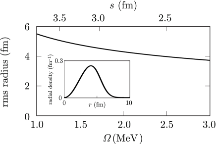
Figure 1: Calculated ${\bar{r}}$ as a function of $\Omega$ and the radial density distribution for $\Omega$=2.14 MeV (inset) of the Hoyle state. Upper horizontal axis indicates rms radius $s=\sqrt{3/2m\Omega}$ of the $0$s orbit of the external harmonic oscillator potential.

III Parameters and numerical calculations

In the calculations, we take a phenomenological Ali–Bodmer potential for $V_{\alpha-\alpha}^{\mathrm{Nucl}}(r)$, which is characterized by the four parameters Ali1966 ,

$$V_{\alpha-\alpha}^{\mathrm{Nucl}}(r)=V_{r}\,e^{-\mu_{r}^{2}r^{2}}-V_{a}\,e^{-\mu_{a}^{2}r^{2}}\,,$$ (14)

where $V_{r}$ and $V_{a}$ are the strengths of the repulsive and attractive parts, respectively, and $\mu_{r}$ and $\mu_{a}$ the corresponding inverse ranges. This potential was obtained by fitting the s-wave phase shifts of $\alpha$–$\alpha$ scattering and has been used in three-$\alpha$ cluster structure studies of ¹²C Yamada2004 . It has been a well-known fact that the Ali–Bodmer local potential does not reproduce the binding energy of the ground state and the Hoyle state. The attraction of the Ali–Bodmer potential is too weak for the three alpha system. One way to reproduce the correct binding of these states is to introduce a strong three-body attracting force Yamada2004 ; Ogasawara1976 ; Lazauskas2011 . Alternatively, in this paper, we introduce an external harmonic potential $V_{\rm ex}(r)=m\Omega^{2}r^{2}/2$ which mimics the three-body attracting force to bind the Hoyle state. Here, $\Omega$ is a fit parameter which corresponds to the strength of the three-body force. The introduction of the external potential makes the theoretical analysis simpler without losing the self-binding essence. If we took only the interaction among the alpha particles, the original translational symmetry would be spontaneously broken in the formation of the nucleus. Then we would have an additional NG mode associated with the translational symmetry in addition to the one of the phase symmetry. To avoid this complexity, we explicitly break the translational symmetry by introducing the external potential. The Coulomb potential, $V_{\alpha-\alpha}^{\mathrm{Coul}}(r)$, is taken as $(4e^{2}/r)\mathrm{erf}(\sqrt{3}r/2b)$, where the size parameter of the $\alpha$ particle $b$ is 1.44 fm.

We attempt to calculate the rms radius, denoted by ${\bar{r}}=\sqrt{\langle r^{2}\rangle}$, and density profile of the Hoyle state from $\xi(\bm{x})$  taking the parameter set $d_{0}$ in Ref. Ali1966 with the proviso that the parameter $V_{r}$ decreases slightly from 500 MeV to 422 MeV, which is consistent with the finding in Ref.Tohsaki1980 that the $\alpha$–$\alpha$ interaction in the three-$\alpha$ system is more attractive than that determined in free $\alpha$–$\alpha$ scattering. The results are shown in Fig. 1. The Hoyle state is found to be dilute for all the $\Omega$ values. The peak position of the radial density distribution, located around 4 $\sim$ 5 fm, and ${\bar{r}}$ are not very sensitive to $\Omega$.

The coexistence of concentration by the trapping potential and repulsion by the self-interaction is crucial for a stable BEC of trapped cold atoms. As a typical counterexample, the trapped BEC of attractively interacting atoms collapses. We therefore regard $\Omega$ and $V_{r}$ as the key parameters in our study, and fit them below with the fixed $V_{a}=130$ MeV, $\mu_{a}=0.475$ fm^-1, and $\mu_{r}=0.7$ fm^-1 in the parameter set $d_{0}$ Ali1966 .

IV Energy spectrum

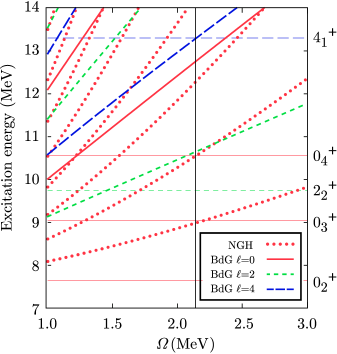
Figure 2: (Color online) NGH (dotted lines) and BdG (solid or dashed lines) excitation energies with $\ell=0$ (red), 2 (green), and 4 (blue) as a function of $\Omega$ when $V_{r}=422$ MeV is fixed. The horizontal lines indicate the excitation energies of the observed $\alpha$ cluster states in ¹²C Itoh2011 ; Freer2009 ; Zimmerman2011 ; Zimmerman2013 ; Itoh2013 ; Freer2011 , and the vertical line is a guide to the eye.

Figure 3: The calculated energy levels for parameter set A ($\Omega=$2.14 MeV, $V_{r}=$422 MeV), compared with the observed $\alpha$ cluster states in ¹²C Itoh2011 ; Freer2009 ; Zimmerman2011 ; Zimmerman2013 ; Itoh2013 ; Freer2011 .

First we use only the existing experimental energy levels to determine the two fit parameters $\Omega$ and $V_{r}$ .The $\Omega$-dependence of the calculated energy levels is given in Fig. 2. Fig. 3 shows the calculated energy levels for the best fitting parameters $\Omega=2.14$ MeV and $V_{r}=422$ MeV, which is referred to as the parameter set A, in comparison with the observed $\alpha$ cluster states. The calculated ${\bar{r}}$ of 0${}_{2}^{+}$ is 4.21fm, which is comparable with the calculations in Refs.  Uegaki1977 ; Tohsaki2001 ; Yamada2005 ; Kurokawa2007 . The agreement between the calculated and experimental energy levels is good, and the order of the levels is correctly reproduced. Our calculation reproduces the two $0^{+}$ NGH states $(\nu=1,2)$ , which correspond well to the $0_{3}^{+}$ at 9.04 MeV and $0_{4}^{+}$ at 10.56 MeV, respectively. The existence of the NGH states is critical for the assignments, because there is no BdG state with $\ell=0$ near the energies of $0_{3}^{+}$ and $0_{4}^{+}$. Then, quite naturally, the excitations $2_{2}^{+}$ and $4_{1}^{+}$ are identified as the BdG states with $\ell=2,4$. All the observed positive parity states are well reproduced as BEC states of $\alpha$ clusters. This shows that the present field theory is useful even for a few-body system.

In Figs. 2 and 3, the calculation shows two $0^{+}$ states around $12.5\mathrm{MeV}$, where no corresponding excitation has been established experimentally yet. These are the NGH state with $\nu=3$, $\bigl{|}\Psi_{3}\bigr{\rangle}\bigl{|}0\bigr{\rangle}_{\mathrm{ex}}$, and the BdG state $\bigl{|}\Psi_{0}\bigr{\rangle}({\hat{a}}^{\dagger}_{100}\bigl{|}0\bigr{\rangle}_{\mathrm{ex}})$, denoted simply as $\bigl{|}\rm h\bigr{\rangle}$ and $\bigl{|}\rm BdG\bigr{\rangle}$, respectively. Because the energy difference between the two states is small and the interaction Hamiltonian allows mutual transitions, they mix with each other to make new two energy eigenstates. A rough estimation of diagonalizing ${\hat{H}}$ in the subspace of $\bigl{|}\rm h\bigr{\rangle}$ and $\bigl{|}\rm BdG\bigr{\rangle}$ gives the eigenstates, $0.98\bigl{|}\rm BdG\bigr{\rangle}-0.18\bigl{|}\rm h\bigr{\rangle}$ with an energy of $12.60\mathrm{MeV}$ and $0.98\bigl{|}\rm h\bigr{\rangle}+0.18\bigl{|}\rm BdG\bigr{\rangle}$ with $12.20\mathrm{MeV}$ . The mixing is not remarkable here, but is generally sensitive to the energy difference. We also note that doubly excited states, e.g., $\bigl{|}\Psi_{1}\bigr{\rangle}({\hat{a}}^{\dagger}_{02m}\bigl{|}0\bigr{\rangle}_{\mathrm{ex}})$ are possible.

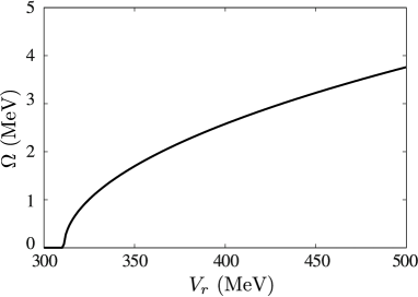
Figure 4: $V_{r}$-$\Omega$ plot for ${\bar{r}}=3.8\,\mathrm{fm}$

Next, we try to determine the parameters $\Omega$ and $V_{r}$ in another way. First of all, because the observed energy levels have large widths, their fitting is not very useful. We add the rms radius of the Hoyle state, depending on the wave function, as an object to be fitted. The value of ${\bar{r}}=4.21\,\mathrm{fm}$, calculated for the parameter set A, is rather large, compared with the typical range $3.3\,\sim\,3.8\,\mathrm{fm}$ obtained in other $\alpha$ cluster model calculations Tohsaki2001 ; Fukushima1977 ; Uegaki1977 ; Kanada2007 ; Matsmura2004 , and the values around $2.9\,\mathrm{fm}$ estimated from inelastic scattering from the Hoyle state Danilov2009 . We seek values of the parameters that give energy levels consistent with the observed energy levels, fixing ${\bar{r}}$. The plot in Fig. 4 represents a constraint when ${\bar{r}}$ is fixed to be $3.8\,\mathrm{fm}$ . We point out the following two facts in this parameter search. Firstly, we have negative $E_{\nu}$ for $V_{r}<370\,\mathrm{MeV}$ and complex $\omega_{120}$ for $V_{r}<330\,\mathrm{MeV}$, implying that BEC is unstable for smaller $V_{r}$ (consequently smaller $\Omega$). The former is caused by the negative “mass” $1/(I-4C_{1102})<0$ in Eq. (II). The latter is the dynamical instability Pu1999 ; Garay2000 ; Skryabin2000 ; Wu2003 ; Mettenen2003 ; Kawaguchi2004 ; Mine2007 , and occurs, because the weak repulsive interaction cannot prevent BEC from collapsing. Secondly, $\Omega$ is the most significant parameter to determine the energy level spacing, and large $\Omega$ ($>3\,\mathrm{MeV}$) cannot reproduce the observed energy levels. After all, no solution is found for the small ${\bar{r}}$ that requires large $\Omega$. We therefore advance our calculations, taking the maximum ${\bar{r}}=3.8\,\mathrm{fm}$. Fig. 5 indicates the $V_{r}$-dependence of calculated energy levels. Choosing the best fitting parameters $\Omega=2.58\,\mathrm{MeV}$ and $V_{r}=400\,\mathrm{MeV}$, called the parameter set B, we give the results of calculated energy levels in Fig. 6. The zero energy spacing are narrower due to the smaller $V_{r}$ and the BdG energy spacing is wider due to the larger $\Omega$ than those in Fig. 3. As a result, the NGH state with $\nu=4$ is located near $4^{+}_{1}$, while the energy level of the NGH state with $\nu=3$ falls down to the midpoint between $0_{4}^{+}$ and $4^{+}_{1}$, and the calculated BdG excitation levels tend to be above the observed levels.

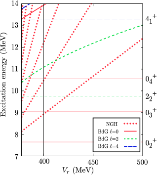
Figure 5: (Color online) NGH (dotted lines) and BdG (solid or dashed lines) excitation energies with $\ell=0$ (red), 2 (green), and 4 (blue) as a function of $V_{r}$ for fixed ${\bar{r}}=3.8\,\mathrm{fm}$.

Figure 6: The calculated energy levels for parameter set B ($\Omega=$2.58 MeV, $V_{r}=$400 MeV).

Our interpretation of the $\alpha$ cluster states as phase locking due to BEC is quite different from the traditional $\alpha$ cluster model, ab initio calculations, and other approaches that try to explain them as collective modes in configuration space, e.g., the rotational band or vibrational states caused by breakdown of rotational or translational symmetries.

In the traditional models, there has been a long-standing question about which excited states are the rotational band members built on the Hoyle state Freer2014 . In other words, which of the $0_{2}^{+}$ and $0_{3}^{+}$ states is the bandhead of the observed $2_{2}^{+}$ and $4_{1}^{+}$ states? The first and traditional $\alpha$ cluster model picture regards the Hoyle state as the bandhead state Freer2012B ; Ogloblin2014 ; Morinaga1956 . In the $\alpha$ condensate model Yamada2005 , the $2_{2}^{+}$ state is interpreted as a state in which an $\alpha$ cluster is lifted from the Hoyle state to the $D$ state in configuration space, and both states have essentially the same weakly coupled [⁸Be($0^{+})\times\alpha$]_J cluster configuration revealed in Refs.Uegaki1977 ; Kurokawa2007 . In these cluster model pictures, because the Hoyle and $2_{2}^{+}$ states have a gas-like spherical structure, it is difficult to consider logically that a rotational band is built. In ab initio lattice Epelbaum2012 and no-core shell model Dreyfuss2013 calculations, the Hoyle, $2_{2}^{+}$, and $4_{1}^{+}$ states are understood to be rotational band states. The second interpretation is that the $0_{3}^{+}$ state is a bandhead state on which the rotational $2_{2}^{+}$ and $4_{1}^{+}$ states are built Freer2012B . Ref.Kurokawa2007 suggests that the $0_{3}^{+}$ state is a higher nodal state with the [⁸Be($0^{+})\times\alpha$($L=0)$]_J=0 structure. A calculated large $B(E2)$ value of the 2${}_{2}^{+}$$\rightarrow$0${}_{3}^{+}$ transition Kanada2007 is reported, although no experimental data are available. In the next section, we will calculate the transition probability and also obtain a large value in our approach.

The reason that these two different interpretations have been presented is entirely due to the appearance of the Hoyle and $0_{3}^{+}$ states so closely above the $\alpha$ threshold. If rotational invariance of the $0_{2}^{+}$ and $0_{3}^{+}$ states in configuration space is broken, a rotational band should appear individually on both the $0_{2}^{+}$ and $0_{3}^{+}$ states, in contradiction with the experimental data. It seems difficult to determine which interpretation is correct as long as these are considered as collective modes with $\alpha$ cluster structure in configuration space. In our picture above, the question does not arise in principle. Our calculations show that the $2_{2}^{+}$ and $4_{1}^{+}$ states are the BdG states and need not be rotational member states on either the Hoyle state or the $0_{3}^{+}$ state. In fact, the $J(J+1)$ plot of the excitation energy of the observed states of the band based on the above two pictures deviates from a straight line.

Why and how does nature allow in principle the emergence of the $0_{4}^{+}$ state, which is interpreted as a linear chain-like $\alpha$ cluster state in Refs.Kurokawa2007 ; Chernykh2007 ; Kanada2007 ; Suhara2014 , so close to the $0_{3}^{+}$ and $0_{2}^{+}$ states? In our picture, the close $0_{3}^{+}$ and $0_{4}^{+}$ states emerge naturally and fundamentally as the NGH states, which is a logical consequence of BEC of the Hoyle state, and the three are closely interrelated.

V $\gamma$ decay

We can calculate the $\gamma$ decay transitions, using the wave functions that have already been obtained. Below the transitions 2${}_{2}^{+}$$\rightarrow$0${}_{2}^{+}$ and 2${}_{2}^{+}$$\rightarrow$0${}_{3}^{+}$ are considered.

The interaction of $\alpha$ particle, treated as a point-like particle with a charge $2e$, with the photon field ${\hat{\bm{A}}}$, is introduced from the gauge principle ${\bm{\nabla}}\rightarrow{\bm{\nabla}}-2ie{\hat{\bm{A}}}$ in the Hamiltonian (II), and the interaction Hamiltonian is given by

$${\hat{H}}_{A} \simeq-\int\!d^{3}x\;{\hat{\bm{j}}}(x)\cdot{\hat{\bm{A}}}(x)\,,$$ (15)

$${\hat{\bm{j}}}(x) =\hat{\psi}^{\dagger}(x)\frac{2e}{im}{\bm{\nabla}}\hat{\psi}(x)\,.$$ (16)

We make a multipole expansion of ${\hat{\bm{A}}}$. The transitions 2${}_{2}^{+}$$\rightarrow$0${}_{2}^{+}$ and 2${}_{2}^{+}$$\rightarrow$0${}_{3}^{+}$ are electric quadrupole transitions, and the decay rate for a general electric transition with a photon angular momentum $J$ is

$${\Gamma}_{fi}({\rm E}:k,J,M)=\frac{8\pi(J+1)}{J((2J+1)!!)^{2}}k^{2J+1}$$

$$\qquad\times\left|\bigl{\langle}f\bigr{|}{\hat{\cal M}}({\rm E}:kJM)\bigl{|}i\bigr{\rangle}\right|^{2}\,,$$ (17)

where $\bigl{|}i\bigr{\rangle}$, $\bigl{|}f\bigr{\rangle}$ represent the initial and final states of th nucleus with respective energies, $E_{i}$ and $E_{f}$, and $k=E_{i}-E_{f}$ is the photon energy. The multipole moment ${\hat{\cal M}}$ Bohr1969 is

$${\hat{\cal M}}({\rm E}:kJM)=\frac{(2J+1)!!}{k^{J+1}}\sqrt{\frac{J}{J+1}}$$

$$\quad\times\int\!d^{3}x\;{\hat{\bm{j}}}(\bm{x})\cdot{\bm{\nabla}}\times\left\{j_{J}(kr){\bm{Y}}_{JJM}(\theta,\varphi)\right\}\,,$$ (18)

where $j_{\ell}$ and ${\bm{Y}}_{JJM}$ are the spherical Bessel function and vector spherical harmonics, respectively. When the initial nuclear state is unpolarized and a sum over the final polarization states is taken, the decay rate is

$${\bar{\Gamma}}_{fi}({\rm E}:k,J)=\frac{8\pi(J+1)}{J((2J+1)!!)^{2}}k^{2J+1}B({\rm E}J:J_{i}\,\rightarrow\,J_{f})$$

$$B({\rm E}J:J_{i}\,\rightarrow\,J_{f})=\frac{1}{2J_{i}+1}$$

$$\qquad\times\left|\bigl{\langle}f(J_{f})\bigr{|}\big{|}{\hat{\cal M}}({\rm E}:kJ)\big{|}\bigl{|}i(J_{i})\bigr{\rangle}\right|^{2}\,,$$ (19)

where $J_{i}$ and $J_{f}$ are the initial and final nuclear spins, respectively, and $B$ is the reduced transition probability Bohr1969 .

Figure 7: Numerical solutions of (a) $\xi(r)$, (b) $\eta(r)$, (c) $\mathcal{U}_{12}(r)\,,\mathcal{V}_{12}(r)$, and (d) $\mathcal{U}_{14}(r)\,,\mathcal{V}_{14}(r)$ for the parameter sets A and B.

Figure 8: Calculated $|\Psi_{\nu}(q)|^{2}$ for the parameter sets A and B.

We calculate ${\bar{\Gamma}}_{fi}$ and $B$ for the transitions 2${}_{2}^{+}$$\rightarrow$0${}_{2}^{+}$ and 2${}_{2}^{+}$$\rightarrow$0${}_{3}^{+}$ . The states 0${}_{2}^{+}$, 0${}_{3}^{+}$, and 2${}_{2}^{+}$ are identified as the vacuum $\bigl{|}\Psi_{0}\bigr{\rangle}\bigl{|}0\bigr{\rangle}_{\mathrm{ex}}$, the NGH state $\bigl{|}\Psi_{1}\bigr{\rangle}\bigl{|}0\bigr{\rangle}_{\mathrm{ex}}$, and the BdG state $\bigl{|}\Psi_{0}\bigr{\rangle}({\hat{a}}^{\dagger}_{02m}\bigl{|}0\bigr{\rangle}_{\mathrm{ex}})$, respectively. Substituting $\hat{\psi}=\xi+\hat{\varphi}$ in Eq. (8) into ${\hat{\bm{j}}}$ in (16), we have the following matrix elements,

$$\bigl{\langle}f(J_{f}=0,M_{f}=0)\bigr{|}{\hat{\cal M}}({\rm E}:k20)\bigl{|}i(J_{i}=2,M_{i}=0)\bigr{\rangle}$$

$$=\frac{30e}{imk^{3}}\sqrt{\frac{2}{3}}\int\!d^{3}x\;\bigl{\langle}\left\{\begin{matrix}\Psi_{0}\\ \Psi_{1}\end{matrix}\right\}\bigr{|}\left\{\left(1+i\hat{Q}\right)\xi(\bm{x})+\hat{P}\eta(\bm{x})\right\}$$

$$\quad\times{\bm{\nabla}}u_{120}(\bm{x})+v_{120}(\bm{x}){\bm{\nabla}}\left\{\left(1-i\hat{Q}\right)\xi(\bm{x})+\hat{P}\eta(\bm{x})\right\}$$

$$\quad\bigl{|}\Psi_{0}\bigr{\rangle}\cdot{\bm{\nabla}}\times\left\{j_{2}(kr){\bm{Y}}_{220}(\theta,\varphi)\right\}\,,$$ (20)

which are further simplified for 2${}_{2}^{+}$$\rightarrow$0${}_{2}^{+}$ as

$$\bigl{\langle}f(0,0)\bigr{|}{\hat{\cal M}}({\rm E}:k20)\bigl{|}N(2,0)\bigr{\rangle}$$

$$\qquad=\frac{60e}{mk^{3}}\int\!dr\,r\left[\xi(r)\left\{\frac{d}{dr}\mathcal{U}_{12}(r)j_{2}(kr)\right.\right.$$

$$\qquad\qquad\quad\left.+\mathcal{U}_{12}(r)\left(\frac{j_{2}(kr)}{r}+kj^{\prime}_{2}(kr)\right)\right\}$$

$$\qquad\quad\qquad\left.+\frac{d}{dr}\xi(r)\mathcal{V}_{12}(r)j_{2}(kr)\right]\,,$$ (21)

and for 2${}_{2}^{+}$$\rightarrow$0${}_{3}^{+}$ as

$$\bigl{\langle}f(0,0)\bigr{|}{\hat{\cal M}}({\rm E}:k20)\bigl{|}i(2,0)\bigr{\rangle}$$

$$=\frac{60e}{mk^{3}}\int\!dr\,r\left[\left\{i\bigl{\langle}\Psi_{1}\bigr{|}\hat{Q}\bigl{|}\Psi_{0}\bigr{\rangle}\xi(r)+\bigl{\langle}\Psi_{1}\bigr{|}\hat{P}\bigl{|}\Psi_{0}\bigr{\rangle}\eta(r)\right\}\right.$$

$$\times\left\{\frac{d}{dr}\mathcal{U}_{12}(r)j_{2}(kr)+\mathcal{U}_{12}(r)\left(\frac{j_{2}(kr)}{r}+kj^{\prime}_{2}(kr)\right)\right\}$$

$$+\left\{i\bigl{\langle}\Psi_{1}\bigr{|}\hat{Q}\bigl{|}\Psi_{0}\bigr{\rangle}\frac{d}{dr}\xi(r)+\bigl{\langle}\Psi_{1}\bigr{|}\hat{P}\bigl{|}\Psi_{0}\bigr{\rangle}\frac{d}{dr}\eta(r)\right\}$$

$$\qquad\left.\times\mathcal{V}_{12}(r)j_{2}(kr)\right]\,.$$ (22)

Here note that $\bigl{\langle}\Psi_{0}\bigr{|}{\hat{Q}}\bigl{|}\Psi_{0}\bigr{\rangle}=\bigl{\langle}\Psi_{0}\bigr{|}{\hat{P}}\bigl{|}\Psi_{0}\bigr{\rangle}=0$ but $\bigl{\langle}\Psi_{1}\bigr{|}{\hat{Q}}\bigl{|}\Psi_{0}\bigr{\rangle}\,,\,\bigl{\langle}\Psi_{1}\bigr{|}{\hat{P}}\bigl{|}\Psi_{0}\bigr{\rangle}\neq 0$, and that the radial functions are defined as

$$\left\{\begin{matrix}\xi(\bm{x})\\ \eta(\bm{x})\end{matrix}\right\}=\left\{\begin{matrix}\xi(r)\\ \eta(r)\end{matrix}\right\}Y_{00}(\theta,\varphi)\,,$$

$$\left\{\begin{matrix}u_{nJM}(\bm{x})\\ v_{nJM}(\bm{x})\end{matrix}\right\}=\left\{\begin{matrix}\mathcal{U}_{nJ}(r)\\ \mathcal{V}_{nJ}(r)\end{matrix}\right\}Y_{JM}(\theta,\varphi)\,.$$ (23)

Using the numerical solutions, $\xi(r)\,,\,\eta(r),\mathcal{U}_{12}(r)\,,\,\mathcal{V}_{12}(r)$ and $\Psi_{\nu}(q)=\bigl{\langle}q\big{|}\Psi_{\nu}\bigr{\rangle}$ ($\nu=0,1$) for each of the parameter sets A and B, we obtain the reduced transition probabilities that are summarized in Table 1. The solutions for each parameter set are shown in Figs. 7 and 8.

Table 1: Calculated reduced transition probabilities $B({\rm E}2:2\,\rightarrow\,0)$ in unit of $e^{2}\,{\rm fm}^{4}$: Ref. Kanada2007 , Ref. Funaki2015 , and our results for the parameter sets A and B.

Transition	Ref. Kanada2007	Ref. Funaki2015	Ours (A)	Ours (B)
$2_{2}^{+}\,\rightarrow\,0_{2}^{+}$	100	295-340	290	204
$2_{2}^{+}\,\rightarrow\,0_{3}^{+}$	310	88-220	342	187

It is remarked that the process $2_{2}^{+}\,\rightarrow\,0_{3}^{+}$ is the transition between the NGH states, whereas the process $2_{2}^{+}\,\rightarrow\,0_{2}^{+}$ is the transition between the BdG states. The physical picture of condensation in our approach implies that the widths of the wave functions, especially $\eta(r)$ and $\mathcal{U}_{12}(r)$, are large. But the final results of $B({\rm E}2:2\,\rightarrow\,0)$ are comparable with those in the other calculations, as in Table 1.

VI Summary

To summarize, we have studied the $\alpha$ cluster structure above the $\alpha$ condensate Hoyle state in ¹²C by formulating an effective field theory of $\alpha$ cluster condensation that properly treats spontaneous symmetry breaking of the global phase. The observed well-developed $\alpha$ cluster states, i.e., the $0_{3}^{+}$ (9.04 MeV), $2_{2}^{+}$ (9.75 MeV), $0_{4}^{+}$ (10.56 MeV), and $4_{1}^{+}$ (13.3 MeV) states, are well reproduced. Then, the emergence of the NGH states just above the Hoyle state is essential. The fact that excitation energies of the BdG and NGH states are the almost same order of magnitude in our calculation is also important for the energy spectrum of ¹²C. We adopted the two parameter sets, and both are consistent with the observed spectrum that has large widths of the energy levels.

We also calculated the $\gamma$ transitions, using the obtained wave functions. Our results of the reduced transition probabilities are compared with those of the other model calculations, and are consistent with the latter.

Although the $\alpha$ cluster condensation involves the small number of $\alpha$ particles, it is stable in our study. This is not true in general, and actually, when the repulsive interaction is weak, we have negative energy of the NGH state and complex energy of the BdG state that indicate an instability of the condensation.

It would be also intriguing to study the NGH states in other nuclei such as ¹⁶O, ²⁰Ne, and ⁴⁰Ca.

- (1) E. A. Cornell and C. E. Wieman, Rev. Mod. Phys. 74, 875 (2002).
- (2) E. Uegaki, S. Okabe, Y. Abe, and H. Tanaka, Prog. Theor. Phys. 57, 1262 (1977); E. Uegaki, Y. Abe, S. Okabe, and H. Tanaka, Prog. Theor. Phys. 62, 1621 (1979).
- (3) A. Tohsaki, H. Horiuchi, P. Schuck, and G. Ropke, Phys. Rev. Lett. 87, 192501 (2001).
- (4) T. Yamada and P. Schuck, Phys. Rev. C 69, 024309 (2004).
- (5) S. Ohkubo and Y. Hirabayashi, Phys. Rev. C 70, 041602 (R) (2004); Sh. Hamada, Y. Hirabayashi, N. Burtebayev, and S. Ohkubo, Phys. Rev. C 87, 024311 (2013).
- (6) T. Yamada and P. Schuck, Eur. Phys. J. A 26, 185 (2005).
- (7) C. Kurokawa and K. Katō, Phys. Rev. C 71, 021301 (2005); Nucl. Phys. A 738, 455c (2004).
- (8) C. Kurokawa and K. Katō, Nucl. Phys. A 792, 87 (2007).
- (9) Y. Kanada-En’yo, Prog. Theor. Phys. 117, 655 (2007).
- (10) M. Chernykh, H. Feldmeier, T. Neff, P. vonNeumann-Cosel, and A. Richter, Phys. Rev. Lett. 98, 032501 (2007).
- (11) R. Roth, J. Langhammer, A. Calci, S. Binder, and P. Navratil, Phys. Rev. Lett. 107, 072501 (2011).
- (12) A. C. Dreyfuss, K. D. Launey, T. Dytrych, J. P. Draayer, and C. Bahri, Phys. Lett. B 727, 515 (2013).
- (13) E. Epelbaum, H. Krebs, T. A. Lahde, D. Lee, and Ulf-G. Meissner, Phys. Rev. Lett. 109, 252501 (2012).
- (14) M. Freer et al., Phys. Rev. C 80, 041303(R) (2009).
- (15) M. Itoh et al., Nucl. Phys. A 738, 268 (2004); M. Itoh et al., Phys. Rev. C 84, 054308 (2011).
- (16) W. R. Zimmerman, N. E. Destefano, M. Freer, M. Gai, and F. D. Smit, Phys. Rev. C 84, 027304 (2011).
- (17) W. R. Zimmerman et al., Phys. Rev. Lett. 110, 152502 (2013).
- (18) M. Itoh et al., J. Phys.: Conf. Ser. 436, 012006 (2013).
- (19) M. Freer et al., Phys. Rev. C 83, 034314 (2011).
- (20) A. A. Ogloblin et al., EPJ Web Conf. 66, 02074 (2014).
- (21) M. Freer and H. O. U. Fymbo, Prog. Part. Nucl. Phys. 78, 1 (2014).
- (22) P. Ring and P. Schuck, The Nuclear Many-body Problem, (Springer-Verlag, Berlin, 1980).
- (23) J. P. Blaizot and G. Ripka, Quantum Theory of Finite Systems, (MIT press, Cambridge, 1985).
- (24) H. Watanabe and H. Murayama, Phys. Rev. Lett. 108, 251602 (2012); Y. Hidaka, Phys. Rev. Lett. 110, 091601 (2013).
- (25) Y. Nambu and G. Jona-Lasinio, Phys. Rev. 122, 345 (1961).
- (26) J. Goldstone, Nuovo Cimento 19, 154 (1961).
- (27) K. Kadowaki, I. Kakeya, and K. Kindo, Europhys. Lett. 42, 203 (1998).
- (28) P. B. Littlewood and C. M. Varma, Phys. Rev. Lett. 47, 811 (1981); P. B. Littlewood and C. M. Varma, Phys. Rev. B 26, 4883 (1982).
- (29) C. M. Varma, J. Low Temp. Phys. 126, 901 (2001).
- (30) R. A. Broglia, O. Hansen, and C. Riedel, Adv. Nucl. Phys. 6, 259 (1973); R. A. Broglia, J. Terasaki, and N. Giovanardi, Phys. Rep. 335, 1 (2000); D. M. Brink and R. A. Broglia, Nuclear Superfluidity: Pairing in Finite Systems (Cambridge University Press, Cambridge, 2005).
- (31) ATLAS Collaboration, Phys. Lett. B 716, 1 (2012); CMS Collaboration, Phys. Lett. B 716, 30 (2012).
- (32) R. Matsunaga, Y. I. Hamada, K. Makise, Y. Uzawa, H. Terai, Z. Wang, and R. Shimano, Phys. Rev. Lett. 111, 057002 (2013).
- (33) S. Ohkubo, arXiv: nucl-th 1301.7485 (2013).
- (34) Y. Nakamura, J. Takahashi, and Y. Yamanaka, Phys. Rev. A 89, 013613 (2014).
- (35) S. Ali and A. R. Bodmer, Nucl. Phys. A 80, 99 (1966).
- (36) E. P. Gross, Nuovo Cimento 20, 454 (1961); J. Math. Phys. 4, 195 (1963); L. P. Pitaevskii, Zh. Eksp. Teor. Fiz. 40, 646 (1961).
- (37) M. Lewenstein and L. You, Phys. Rev. Lett. 77, 3489 (1996).
- (38) H. Matsumoto and S. Sakamoto, Prog. Theor. Phys. 107, 679 (2002).
- (39) N. N. Bogoliubov, J. Phys. (Moscow) 11, 32 (1947).
- (40) P. G. de Gennes, Superconductivity of Metals and Alloys (Benjamin, New York, 1966).
- (41) E.R. Marshalek and J. Weneser, Ann. Phys. 53, 569 (1969).
- (42) H. Ogasawara and J. Hiura, Prog. Theor. Phys. 59, 655 (1978).
- (43) R. Lazauskas and M. Dufour, Phys. Rev. C 84, 064318 (2011).
- (44) A. Tohsaki-Suzuki, M. Kamimura, and K. Ikeda, Prog. Theor. Phys. Suppl. 68, 359 (1978).
- (45) M. Kamimura, Nucl. Phys. A 351, 456 (1981).
- (46) H. Matsumura and Y. Suzuki, Nucl. Phys. A 739, 238 (2004).
- (47) A. N. Danilov, T. L. Belyaeva, A. S. Demyanova, S. A. Goncharov, and A. A Ogloblin, Phys. Rev. C 80, 054603 (2009).
- (48) H. Pu, C. K. Law, J. H. Eberly, and N. P. Bigelow, Phys. Rev. A 59, 1533 (1999).
- (49) L. J. Garay, J. R. Anglin, J. I. Cirac, and P. Zoller, Phys. Rev. Lett. 85, 4643, (2000); Phys. Rev. A 63, 023611 (2001).
- (50) D. V. Skryabin, Phys. Rev. A. 63, 013602 (2000).
- (51) B. Wu and Q. Niu, New J. Phys. 5, 104 (2003).
- (52) M. Möttönen, T. Mizushima, T. Isoshima, M. M. Salomaa, and K. Machida, Phys. Rev. A 68, 023611 (2003).
- (53) Y. Kawaguchi and T. Ohmi, Phys. Rev. A. 70, 043610 (2004).
- (54) M. Mine, M. Okumura, T. Sunaga and Y. Yamanaka, Ann. Phys. 322, 2327 (2007).
- (55) M. Freer, J. Phys.: Conf. Ser. 436, 012002 (2013).
- (56) H. Morinaga, Phys. Rev. 101, 254 (1956).
- (57) T. Suhara, Y. Funaki, B. Zhou, H. Horiuchi, and A. Tohsaki, Phys. Rev. Lett. 112, 062501 (2014).
- (58) A. Bohr and B. R. Mottelson, Nuclear Structure Vol. I, (Benjamin, New York, 1969).
- (59) Y. Funaki, Phys. Rev. C 92, 021302(R) (2015).