Normalized entropy versus volume
for pseudo-Anosovs

Abstract.

Thanks to a recent result by Jean-Marc Schlenker, we establish an explicit linear inequality between the normalized entropies of pseudo-Anosov automorphisms and the hyperbolic volumes of their mapping tori. As its corollaries, we give an improved lower bound for values of entropies of pseudo-Anosovs on a surface with fixed topology, and a proof of a slightly weaker version of the result by Farb, Leininger and Margalit first, and by Agol later, on finiteness of cusped manifolds generating surface automorphisms with small normalized entropies. Also, we present an analogous linear inequality between the Weil-Petersson translation distance of a pseudo-Anosov map (normalized by multiplying the square root of the area of a surface) and the volume of its mapping torus, which leads to a better bound.

1. Introduction

Let $\varSigma=\varSigma_{g,m}$ be an orientable surface of genus $g$ with $m$ punctures. We will suppose that $3g-3+m\geq 1$ so that $\varSigma$ admits a Riemannian metric of constant curvature $-1$, a hyperbolic structure of finite area, which, by Gauss-Bonnet, satisfies $\mathrm{Area}\,\varSigma=2\pi|\chi(\varSigma)|=2\pi(2g-2+m)$ with respect to the hyperbolic metric.

The isotopy classes of orientation preserving automorphisms of $\varSigma$, called mapping classes, were classified into three families by Nielsen and Thurston [23], namely periodic, reducible and pseudo-Anosov. Choose a representative $h$ of a mapping class $\varphi$, and consider its mapping torus,

$$\varSigma\times[0,1]/(x,1)\sim(h(x),0).$$

Since the topology of the mapping torus depends only on the mapping class $\varphi$, we denote its topological type by $N_{\varphi}$

A celebrated theorem by Thurston [24] asserts that $N_{\varphi}$ admits a hyperbolic structure iff $\varphi$ is pseudo-Anosov. By Mostow-Prasad rigidity a hyperbolic structure of finite volume in dimension 3 is unique and geometric invariants are in fact topological invariants. In [12], Kin, Takasawa and the first named author compared the hyperbolic volume of $N_{\varphi}$, denoted by $\mathrm{vol}\,N_{\varphi}$, with the entropy of $\varphi$, denoted by $\mathrm{ent}\,\varphi$. By entropy we mean the infimum of the topological entropy of automorphisms isotopic to $\varphi$. In particular, they proved that there is a constant $C(g,m)>0$ depending only on the topology of $\varSigma$ such that

$$\mathrm{ent}\,\varphi\geq C(g,m)\,\mathrm{vol}N_{\varphi}.$$

This result only asserts the existence of a constant $C(g,m)$ since the proof is based on a result of Brock [5] involving several constants for which, a priori, it appears difficult to compute sharp values. On the other hand, it is well known that the infimum of $\mathrm{ent}\,\varphi/\mathrm{vol}\,N_{\varphi}$ is $0$. In fact, Penner constructed examples [19] which demonstrate that, as the complexity of surface increases, the entropy of a pseudo-Anosov can be arbitrarily close to $0$. By Jørgensen-Thurston Theory [22], the infimum of volumes of hyperbolic 3-manifolds is strictly positive so $C(g,m)$ necessarily tends to $0$ when $g+m\to\infty$.

Our main theorem gives an explicit value for $C(g,m)$

Theorem 1.

The inequality,

$${\rm ent}\,\varphi\geq\frac{1}{3\pi|\chi(\varSigma)|}\,{\rm vol}\,N_{\varphi},$$ (1.1)

or equivalently,

$$2\pi|\chi(\varSigma)|\,{\rm ent}\,\varphi\geq\frac{2}{3}\,{\rm vol}\,N_{\varphi}$$ (1.2)

holds for any pseudo-Anosov $\varphi$.

The quantity appearing on the left hand side of (1.2) is often referred to as the normalized entropy. The main theorem can thus be restated informally: “the normalized entropy over the volume is bounded from below by a psoitive constant which does not depend on the topology of $\varSigma$”.

The value of $C(g,m)$ above does not seem to be quite far from the sharp constant. For example, choose the case that the surface is the punctured torus, so that $g=1,\,m=1$ and $|\chi(\varSigma_{1,1})|=1$. Then the inequality (1.1) becomes

$$\frac{{\rm ent}\,\varphi}{{\rm vol}\,N_{\varphi}}\geq\frac{1}{3\pi}=0.10610\dots$$

In this particular case, it is conjectured (see Conjecture 6.10 in [12] with supporting evidence) that

$$\frac{{\rm ent}\,\varphi}{{\rm vol}\,N_{\varphi}}\geq\frac{\log\frac{3+\sqrt{5}}{2}}{2v_{3}}=0.47412\dots,$$

where $v_{3}=1.01494\dots$ is the volume of the hyperbolic regular ideal simplex. The conjectured constant above is known to be attained by the figure eight knot complement which admits a unique $\varSigma_{1,1}$-fibration.

The first application of Theorem 1, is an amelioration of the lower bound,

$$\mathrm{ent}\,\varphi\geq\frac{\log 2}{4(3g-3+m)},$$

for the entropy of pseudo-Anosovs on a surface due to Penner[19], provided that there is at least one puncture.

Corollary 2.

Let $\varphi$ be a pseudo-Anosov on $\varSigma_{g,m}$ with $m\geq 1$. Then

$$\mathrm{ent}\,\varphi\geq\frac{2v_{3}}{3\pi|\chi(\varSigma)|}=\frac{2v_{3}}{3\pi(2g-2+m)}.$$

Proof.

It is known by Cao and Meryerhoff in [7] that the smallest volume of an orientable noncompact hyperbolic 3-manifold is attained by the figure eight knot complement and it is $2v_{3}$. Thus replacing ${\rm vol}\,N_{\varphi}$ in (1.1) by $2v_{3}$, we obtain the estimate. ∎

If a manifold admits a fibration over the circle, its first Betti number is necessarily positive. It is conjectured that the smallest volume of a hyperbolic $3$-manifold with positive first Betti number is also $2v_{3}$. If it were true, then we could drop the assumption on the number of punctures “ $m\geq 1$” in Corollary 2.

The second application of our main theorem is the proof of a slightly weaker form of Farb, Leininger and Margalit’s finiteness theorem for small dilitation pseudo Anosovs.

Corollary 3 (Farb, Leininger and Margalit [10], Agol [1]).

For any $C>0$, there are finitely many cusped hyperbolic $3$-manifolds $M_{k}$ such that any pseudo-Anosov $\varphi$ on $\varSigma$ with $|\chi(\varSigma)|\,{\rm ent}\,\varphi<C$ can be realized as the monodromy of a fibration on a manifold obtained from one of the $M_{k}$ by an appropriate Dehn filling.

We note that Farb, Leininger and Margalit are able to obtain in addition that the $M_{k}$ are in fact fibered and the surgeries (fillings) are along suspensions of punctures of the fiber.

Proof.

If $|\chi(\varSigma)|\,{\rm end}\,\varphi$ is bounded from above by a constant $C$, then it certainly bounds the volume of $N_{\varphi}$ by Theorem 1. Recall that the thin part of $N_{\varphi}$ consists of neighborhoods of (rank 2) cusps and Margulis tubes around short geodesics all pairwise disjoint. Thus the boundary of the thick part, that is the complement of the thin part, consists of finitely many tori and $N_{\varphi}$ is obtained from the thick part by Dehn filling these. The volume of $N_{\varphi}$ bounds the volume of the thick part and, using a covering by (finitely many) metric balls, Jorgensen and Thurston [22] have shown that there are only finitely many possibilities for its topological type. ∎

Finally, replacing the entropy by Weil-Petersson translation distance in the proof of Theorem 1, yields an explicit value for the constant appearing in the upper bound for volume of the mapping torus in Brock’s Theorem 1.1 [5].

Corollary 4.

If $\varSigma$ is compact, then, the inequality,

$$||\varphi||_{{\rm WP}}\geq\frac{2}{3\sqrt{2\pi|\chi(\varSigma)|}}\,{\rm vol}\,N_{\varphi},$$

or equivalently,

$$\sqrt{2\pi|\chi(\varSigma)|}\,||\varphi||_{{\rm WP}}\geq\frac{2}{3}\,{\rm vol}\,N_{\varphi}$$

holds for any pseudo-Anosov $\varphi$, where $||\cdot||_{{\rm WP}}$ is the Weil-Petersson translation distance of $\varphi$.

It was pointed out to the authors by McMullen that there is a family of pseudo-Anasov automorphisms $\varphi_{k}$ such that $||\varphi_{k}||_{{\rm WP}}$ are bounded whilst the entropy of $\varphi_{k}$, which is just the translation distance for the Teichmüller metric, diverges. In fact, one can construct such examples so that the mapping tori $N_{\varphi_{k}}$ converge to a cusped hyperbolic 3-manifold (though this limit may not be a surface bundle). This can be interpreted as showing that the relationship between volume and Weil-Petersson distance is stronger than that with the Teichmüller distance. Indeed, Brock has shown that there a lower bound for volume in terms of $||\varphi||_{\rm WP}$ but the method that we present does not as yet extend to prove this.

The proof of Theorem 1 has two main ingredients: The first is Krasnov and Schlenker’s recent results on the renormalized volumes of quasi-Fuchsian manifolds [14, 18]; The second is the work of McMullen [15] and Brock-Bromberg [6] on geometric inflexibility to obtain convergence in Thurston’s Double Limit Theorem. In the next section we review briefly the requisite results of Krasnov and Schlenker and obtain an intermediate inequality (Corollary 12) between the volume of the convex core of a quasi-Fuchsian manifold and Teichmüller distance. In the proceeding section, we prove Theorem 1 and Corollary 4. The last section is an appendix where we present a simplified exposition of the ideas behind geometric inflexibility and a proof of the convergence result stated in Brock [5] which leads to a proof of the main theorem.

Acknowledgement: The authors are indebted to Ian Agol, Martin Bridgemann, Jeff Brock, Ken Bromberg, Dan Margalit, Curt McMullen, Kasra Rafi, Jean-Marc Schlenker and Juan Souto for their valuable suggestions, comments and encouragement without which this paper might never have been completed.

2. preliminaries

2.1. Differentials

Let $R$ be a Riemann surface and $T^{1,0}R$ and $T^{0,1}R$ denote respectively the holomorphic and the anti-holomorophic parts of the complex cotangent bundle, a canonical bundle, over $R$ respectively.

A quadratic differential $q$ on $R$ locally expressed by $q(z)dz^{2}$ is a section of the line bundle $(T^{1,0}R)^{\otimes 2}$. A Beltrami differential $\mu$ on $R$ locally expressed by $\mu(z)\frac{d\bar{z}}{dz}$ is a section of the line bundle $T^{0,1}R\otimes(T^{1,0})^{*}R$ They are main players in Teichmüller theory. A Beltrami differential $\mu$ can be interpreted as a representative of an infinitesimal deformation of complex structure on $R$. Hence, to each $\mu$ there is a corresponding tangent vector to Teichmüller space $\mathcal{T}=\mathcal{T}_{g,m}$ at $R$, however, there is an infinite dimensional subspace that represents the trivial deformation so that the correspondence is not injective. We now describe a construction which allows one to eliminate this ambiguity.

Let $Q(R)$ be the space of holomorphic quadratic differentials. By Riemann-Roch, the dimension of $Q(R)$ is $3g-3+m$, that is, equal to that of $\mathcal{T}$. We define the $L^{1}$-norm on $Q(R)$ by

$$||q||_{1}=\int_{R}|q|.$$

We note that, since it is finite dimensional, all norms on $Q(R)$ are equivalent and we shall compare the $L^{1}$-norm to another norm, tne $L^{\infty}$-norm, in Paragraph 2.6.

Given a Betrami differential $\mu$ and a quadratic differential $q$ the product of $\mu$ and $q$ is a section of the line bundle $T^{0,1}R\otimes T^{1,0}R$, and there is a natural pairing defined by

$$(q,\,\mu)=\int_{R}\mu q.$$

Let $L_{\infty}(R)$ be the space of uniformly bounded Beltrami differentials with respect to the norm,

$$||\mu||_{\infty}=\sup_{\|q\|_{1}=1}|(q,\,\mu)|,$$

namely, $L_{\infty}(R)=\{\mu\,;\,||\mu||_{\infty}<\infty\}$. Define $K$ to be the subspace of $L_{\infty}(R)$

$$K=\{\mu\,;\,(q,\,\mu)=0\;\;\text{for all $q\in Q(R)$}\}.$$

Then $L_{\infty}(R)/K$ can be identified with the tangent space $T_{R}\mathcal{T}$ of the Teichmüller space $\mathcal{T}$ at $R$, and moreover the pairing induces an isomorphism of $Q(R)^{*}$ with $L_{\infty}(R)/K\cong T_{R}\mathcal{T}$. Thus, $Q(R)$ can be regarded as a cotangent space of $\mathcal{T}$ at $R$, $T^{*}_{R}\mathcal{T}$, and $(\;,\;)$ induces the duality pairing,

$$(\;,\;):Q(R)\times L_{\infty}(R)/K\to\mathbb{C}.$$ (2.1)

2.2. Projective Structures

A projective structure on a surface $\varSigma$ is a special type of complex structure being locally modeled on the geometry of the complex projective line $(\widehat{\mathbb{C}},\,\mathrm{PSL}(2,\mathbb{C}))$, where $\widehat{\mathbb{C}}=\mathbb{C}\cup\{\infty\}$ is the Riemann sphere. The projective structure on $\varSigma$ is given by an atlas such that each transition map is the restriction of some element in $\mathrm{PSL}(2,\mathbb{C})$. Clearly these transition maps are holomorphic and so there is a unique complex structure naturally associated to a given projective structure. Let $X$ be a surface homeomorphic to $\varSigma$ together with a projective structure, and let $R$ be its underlying Riemann surface. When $\chi(\varSigma)<0$ there is a bijection between projective structures and holomorphic quadratic differentials. To see this, recall that by the Uniformization Theorem the universal cover of $X$ can be identified with the Poincaré disk $\mathbb{D}=\{z\in\mathbb{C}\,;\,|z|<1\}$. The developing map $f:\widetilde{X}\to\widehat{\mathbb{C}}$ can be regarded as a meromorphic function on $\mathbb{D}$. Now the Schwarzian derivative $S(f)$ of $f$ defines a holomorphic quadratic differential $q$ on $R$. Conversely, given a holomorphic quadratic differential $q$ on $R$, the Schwarzian differential equation

$$S(f)=q$$

has a solution which gives rise to a developing map of some complex projective structure on $R$. Thus, there is a one-to-one correspondence between the set of all complex projective structures on $R$ and $Q(R)$.

2.3. Quasi-Fuchsian Manifolds

A quasi-Fuchsian group is defined to be a discrete subgroup $\Gamma$ of ${\rm PSL}(2,\mathbb{C})$ such that its limit set $L_{\Gamma}$ of $\Gamma$ on the boundary $\partial\mathbb{H}^{3}=S^{2}_{\infty}$ is either a circle or a quasi-circle (an embedded copy of the circle with Hausdorff dimension strictly greater than 1). This definition implies many consequences. For example, the domain of discontinuity $\Omega_{\Gamma}=S^{2}_{\infty}-L_{\Gamma}$ consists of exactly two simply-connencted domains, denoted by $\Omega_{\Gamma}^{+}$ and $\Omega_{\Gamma}^{-}$, the quotients of $\Omega_{\Gamma}^{\pm}$ by $\Gamma$ are the same 2-orbifold $O$ but with opposite orientations, and $\mathbb{H}^{3}/\Gamma$ is a geometrically finite hyperbolic 3-orbifold homeomorphic to $O\times\mathbb{R}$. If $\Gamma$ is torsion free, then $O$ becomes a surface $\varSigma$ and, in particular, $\Gamma$ is isomorphic to the fundamental group of $\varSigma$. In this case we say that the quotient of $\mathbb{H}^{3}$ by the quasi-Fuchsian group $\Gamma$ is a quasi-Fuchsian manifold.

The action of $\Gamma$ on $\Omega_{\Gamma}$ is holomorphic so $X=\Omega_{\Gamma}^{+}/\Gamma$ and $Y=\Omega_{\Gamma}^{-}/\Gamma$ are marked Riemann surfaces. Thus, there is a well defined map taking a quasi-Fuchsian manifold $\mathbb{H}^{3}/\Gamma$ to a pair of marked Riemann surfaces $X,\,Y$ in the Teichmüller space $\mathcal{T}$ of $\varSigma$. In [2] Bers showed that this map has an inverse. He obtains as a corollary a parametrization of the set of quasi-Fuchsian manifolds by the $\mathcal{T}\times\overline{\mathcal{T}}$. In other words, for any pair $(X,Y)\in\mathcal{T}\times\overline{\mathcal{T}}$, there is a unique quasi-Fuchsian manifold $QF(X,Y)$. As noted above, the limit set of a quasi-Fuchsian group is either a circle or a quasi-circle, and the quotient of its convex hull in $\mathbb{H}^{3}$ by $\Gamma$, denoted $C(X,Y)$, is homemorphic to $\varSigma$ or $\varSigma\times[0,\,1]$ accordingly, called the convex core. It is known to be the smallest convex subset homotopy equivalent to $QF(X,Y)$.

Since the action of a quasi-Fuchsian group $\Gamma$ on $\Omega_{\Gamma}$ is linear fractional, the Riemann surfaces $X$ and $Y$ are equipped not only with complex structures but also with complex projective structures. Thus we have associated holomorphic quadratic differentials $q_{X}$ and $q_{Y}$. Let $q$ denote the unique holomorphic quadratic differential on $X\sqcup Y$ such that its restriction to $X$ is $q_{X}$ and to $Y$ is $q_{Y}$.

The notations $q_{X},\,q_{Y}$ may be a bit misleading since they both could vary even if one of complex structures of $X$ or $Y$ stays constant. However, as long as discussing quasi-Fuchsian deformations, we regard $q_{X}$ as a complex projective structure of the Riemann surface on the left and $q_{Y}$ on the right. This convention would resolve confusion of notations.

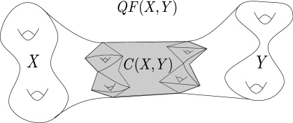
Figure 1. The quasi-Fuchsian manifold, the surfaces at infinity and the convex core.

2.4. Renormalization of Volume

Renormalization of the volume of convex cocompact hyperbolic 3-manifolds were studied extensively by Krasnov and Schlenker in [14]. In the following paragraphs we recall Krasnov and Schlenker’s results focusing on quasi-Fuchsian case. Note that the surface at infinity $\Omega_{\Gamma}/\Gamma$ has 2 connected components.

Throughout the rest of this section, we assume that $\varSigma$ is compact. Let $M$ be a quasi-Fuchsian manifold $\mathbb{H}^{3}/\Gamma$ homeomorphic to $\varSigma\times\mathbb{R}$. Following [14] we say that a codimension-zero smooth compact convex submanifold $N\subset M$ is strongly convex if the normal hyperbolic Gauss map from $\partial N=\partial_{+}N\sqcup\partial_{-}N$ to the boundary at infinity $\Omega_{\Gamma}/\Gamma$ is a homeomorphism. For example, a closed $\varepsilon$-neighborhood of the convex core of a quasi-Fuchsian manifold is strongly convex. Let $S_{0}=\partial N$ then there is a family of surfaces $\{S_{r}\}_{r\geq 0}$ equidistant to $S_{0}$ foliating the ends of $M$. If $g_{r}$ denotes the induced metric on $S_{r}$, then define a metric at infinity associated to the family $\{S_{r}\}_{r\geq 0}$ by

$$g=\lim_{r\to\infty}2e^{-2r}\,g_{r}.$$

The resulting metric $g$ in fact belongs to the conformal class at infinity that is the conformal structure determined by the complex structure on $\Omega_{\Gamma}/\Gamma$. It is easy to see that if we start with a strongly convex submanifold bounded by $S_{r_{0}}$ for some $r_{0}>0$, then the limiting metric is $e^{2r_{0}}g$. Namely, if we shift the parametrization of an equidistant foliation by $r_{0}$, then the limiting metric changes only by scaling $e^{2r_{0}}$.

Conversly, if $g$ is a Riemannian metric in the conformal class at infinity, then Theorem 5.8 in [14] shows that there is a unique foliation of the ends of $M$ by equidistant surfaces with compatible parametrization of leaves starting $r_{0}\geq 0$ so that the associated metric at infinity is equal to $g$. Notice that the parametrization may have to start with a positive $r_{0}$. The construction of a foliation is due to Epstein [8]. Then, a natural quantity to study in the context of strongly convex submanifolds $N\subset M$ is the W-volume defined by

$$W(M,g):=\mathrm{vol}\,N_{r}-\frac{1}{4}\int_{S_{r}}H_{r}\,da_{r}+\pi r\chi(\partial M),$$ (2.2)

where the parametrization $r$ is induced by $g$, $N_{r}$ is a strongly convex submanifold bounded by the associated leaf $S_{r}$, $H_{r}$ is the mean curvature of $S_{r}$ and $da_{r}$ is the induced area form of $S_{r}$. A simple computation which can be found in [18] shows that the W-volume depends only on the metric at infinity $g$, justifying the notation.

The renormalized volume of $M$ is now defined by

$$\mathrm{Rvol}(M):=\sup_{g}W(M,g),$$

where the supremum is taken over all metrics $g$ in the conformal class at infinity such that the area of each surface at infinity $\Omega_{\Gamma}/\Gamma$ with respect to $g$ is $2\pi|\chi(\varSigma)|$. Section 7 in [14] presents an argument, based on the variational formula stated in Corollary 6.2 in [14], that the supremum is in fact uniquely attained by the metric of constant curvature $-1$.

We can now state, in a slightly modified form, that one half of Theorem 1.1 in [18] is as follows.

Theorem 5 (Theorem 1.1 in [18] and its revised version).

Assume that $\varSigma$ is compact. Then, there exists a constant $D=D(\varSigma)>0$ depending only on the topology of $\varSigma$ such that the inequality,

$$\mathrm{vol}\,C(X,Y)\leq\mathrm{Rvol}\,QF(X,Y)+D,$$ (2.3)

holds for any $X,\,Y\in\mathcal{T}$.

2.5. Variational Formula

In [18] the metric at infinity of a quasi-Fuchsian manifold $M$ which attains the renormalized volume is denoted by $\mathrm{I}^{*}$. In particular, the curvature of $\mathrm{I}^{*}$ is constant $-1$. The notation is consistent with the standard one for the first fundamental form. There is also an analogous notion $\mathrm{II}^{*}$ of the second fundamental form on the surface at infinity with the same parametrization with appropriate scaling factor. More precisely, there is a unique bundle morphism $B^{*}$ of the tangent space of boundary, corresponding to the shape operator, which is self-adjoint for $\mathrm{I}^{*}$ and such that

$$\mathrm{II}^{*}=\mathrm{I}^{*}(B^{*}\cdot,\cdot)$$

The variational formula of the renormalized volume involves $\mathrm{II}^{*},\,\mathrm{\dot{I}}^{*}$ and a Riemannian metric of constant curvature $-1$ in the conformal class of the boundary. They all are symmetric $2$-tensors. In general, if we choose a local complex coordinate $z=x+iy$, then we can express a symmetric $2$-tensor using the associated real coordinate $(x,y)$ by $a(dx\otimes dx)+b(dx\otimes dy+dy\otimes dx)+c(dy\otimes dy)$ and hence by a symmetric matrix

$$\begin{pmatrix}a&b\\ b&c\end{pmatrix}.$$

Cororally 6.2 in [14] states the variational formula of the W-volume as follows.

Lemma 6 (Proposition 3.10 [18] and its revised version).

Under a first-order deformation of the hyperbolic structure on $N$,

$$d\,{\rm Rvol}=-\frac{1}{4}\langle\mathrm{II}^{*}_{0},\,\mathrm{\dot{I}}^{*}\rangle$$

holds. Here $\langle\;,\;\rangle$ is the extension to symmetric 2-tensors of the riemannian metric $\rho^{2}|dz|^{2}$ of constant curvature $-1$ defined by

$$\langle A,B\rangle=\int_{R}{\rm tr}\,(G^{-1}AG^{-1}B)\rho^{2}dxdy,$$

where $G$ is the metric tensor, and $\mathrm{II}^{*}_{0}$ is a trace free part of $\mathrm{II}^{*}$.

Krasnov and Schlenker found a remarkable relation between $\mathrm{II}^{*}_{0}$, the trace free part of $\mathrm{II}^{*}$, and the holomorophic quadratic differential $q$ corresponding to the projective structure of the boundary. To see this more precisely, recall that $q$ has a local expression $q=q(z)dz^{2}$ and $q(z)=f(z)+ih(z)$. Then ${\rm Re}\,q=fdx\otimes dx-fdy\otimes dy-h(dx\otimes dy+dy\otimes dx)$ as a symmetric 2-tensor can be expressed by a trace free symmetric matrix

$$\begin{pmatrix}f&-h\\ -h&-f\end{pmatrix}$$

The identity below follows directly from explicit formulae for the holomorphic quadratic differential $q$ in question. Another more geometric proof can also be found in the appendix of [14].

Lemma 7 (Lemma 8.3 in [14]).

$$\mathrm{II}^{*}_{0}=-\mathrm{Re}\,q.$$

Notice that $q=(f+ih)dz^{2}$ can be recovered from $\mathrm{Re}\,q$. Passing through this identification and using an identification of $Q(R)$ with $T_{R}\mathcal{T}$ with respect to the metric $\rho^{2}|dz|^{2}$, the variation of the metric

$$\dot{\mathrm{I}}^{*}=\begin{pmatrix}2\varphi&-2\psi\\ -2\psi&-2\varphi\end{pmatrix}$$

can be transformed to the Beltrami differential

$$\mu=\frac{\varphi-i\psi}{\rho^{2}}\frac{d\bar{z}}{dz}.$$

This leads us to the reinterpration of the variational formula in Lemma 6 in terms of the duality pairing $(\;,\;)$ in (2.1).

Lemma 8.

Under a first-order deformation of the hyperbolic structure on $N$,

$$d\,{\rm Rvol}=-\mathrm{Re}\,(q,\,\mu)=-\int_{R}\mathrm{Re}\,\mu q$$

holds.

Proof.

Fix a local coordinate $z=x+iy$ and let $\rho^{2}|dz|^{2}$ denote the hyperbolic metric then,

$$\langle\mathrm{II}_{0}^{*},\,\dot{\mathrm{I}}^{*}\rangle =\int_{R}\mathrm{tr}(G^{-1}\mathrm{II}_{0}^{*}G^{-1}\dot{\mathrm{I}}^{*})\rho^{2}\,dxdy$$

$$=4\int_{R}(f\varphi+h\psi)\rho^{-2}dxdy$$

$$=4\int_{R}\mathrm{Re}\left(\frac{\varphi-i\psi}{\rho^{2}}(f+ih)\right)dxdy$$

$$=4\int_{R}\mathrm{Re}\,\mu q.$$

∎

2.6. Rvol versus Teichmüller Distance

We start with a quasi-Fuchsian manifold $\mathbb{H}^{3}/\Gamma=QF(X,Y)$. Fix a conformal structure $X$ on the left boundary component, and regard a conformal structure $Y$ on the right as a variable. To each $Y$, we assign an associated complex projective structure on $X$ and therefore a holomorphic quadratic differential $q_{X}$. This defines a map,

$$B_{X}:\mathcal{T}\to Q(X),$$

called a Bers embedding.

Using the hyperbolic metric in the conformal class of $X$, we can measure at each point of $\varSigma$ the norm of $q_{X}$. Let $Q^{\infty}(X)$ be $Q(X)$ endowed with the $L^{\infty}$ norm, namely,

$$||q||_{\infty}=\sup_{x\in X}\frac{|q(x)|}{\rho^{2}(x)},$$

where $\rho|dz|$ defines the hyperbolic metric of constant curvature $-1$.

The following theorem with respect to the hyperbolic metric of constant curvature $-1$, due to Nehari, can be found in a standard text book of the Teichmüller theory such as Theorem 1, p.134 in [11].

Theorem 9 (Nehari [17]).

The image of $B_{X}$ in $Q^{\infty}(X)$ is contained in the ball of radius $3/2$.

Then, consider now the $L^{1}$-norm on $Q(X)$ and denote by $Q^{1}(X)$ the vector space $Q(X)$ endowed with the $L^{1}$ norm.

Corollary 10.

The image of $B_{X}$ in $Q^{1}(X)$ is contained in the ball of radius $3\pi|\chi(\varSigma)|$.

Proof.

The inequality

$$||q||_{1}=\int_{X}|q|=\int_{X}\frac{|q|}{\rho^{2}}\,\rho^{2}\leq||q||_{\infty}\int_{X}\rho^{2}=2\pi|\chi(\varSigma)|\,||q||_{\infty}$$

immediately implies the conclusion. ∎

The proof of the following comparison result is the same as that of Theorem 1.2 in [18] by Schlenker with a different norm.

Proposition 11.

Suppose $\varSigma$ is compact. The inequality,

$${\rm Rvol}\,QF(X,Y)\leq 3\pi|\chi(\varSigma)|\,d_{\rm T}(X,Y),$$ (2.4)

holds for any quasi-Fuchsian manifold $QF(X,Y)$, where $d_{\rm T}$ is the Teichmüller distance on $\mathcal{T}$.

Proof.

Let $Y:[0,d]\to\mathcal{T}$ be the unit speed Teichmüller geodesic joining $X$ and $Y$, so that, in particular, $Y(0)=X,\,Y(d)=Y$ and $d=d_{\rm T}(X,Y)$. Then consider a one-parameter family of quasi-Fuchsian manifolds $\{QF(X,Y(t))\}_{0\leq t\leq d}$. By Lemma 8 the variation under the first-order deformation at time $t$ is given by

$$d\,{\rm Rvol}=\mathrm{Re}\left((q_{X}(t),\dot{X}))+(q_{Y(t)}(t),\dot{Y}(t))\right),$$

where $\dot{X},\,\dot{Y}(t)$ are tangent vectors of the deformation of complex structures on the two ideal boundary components. Since $\dot{X}=0$, integrating the variation of ${\rm Rvol}$ along the path $Y(t)\;(t\in[0,d])$, yields an expression for the renormalised volume

$${\rm Rvol}\,QF(X,Y)=\mathrm{Re}\int_{t=0}^{d}(q_{Y(t)}(t),\dot{Y}(t))dt.$$

On the other hand,

$$|(q_{Y(t)}(t)),\dot{Y}(t))| =\left|\int_{R}q_{Y(t)}(t)\,\dot{Y}(t)\right|$$

$$=\int_{R}|q_{Y(t)}(t)\,\dot{Y}(t)|$$

$$\leq||q_{Y(t)}(t)||_{1}\,||\dot{Y}(t)||_{\infty}$$

where $||\cdot||_{\infty}$ is the supremum norm on $L_{\infty}(Y(t))$ which is the dual to the $L^{1}$-norm on $Q(Y(t))$ and hence an infinitesimal form of the Teichmüller metric. By Corollary 10, for all $t\in[0,d]$ one has ,

$$||q_{Y(t)}(t)||_{1}\leq 3\pi|\chi(\varSigma)|,$$

and, by definition, $||\dot{Y}(t)||_{\infty}=1$ so that the inequality now follows. ∎

Replacing (2.4) in the inequality in Theorem 5 one has,

Corollary 12.

With the notation above,

$$\mathrm{vol}\,C(X,Y)\leq 3\pi|\chi(\varSigma)|\,d_{\rm T}(X,Y)+D$$ (2.5)

3. Proof

We first deal with the case that $\varSigma$ is compact. Let $\varphi$ be a pseudo-Anosov automorphism on $\varSigma$ and choose a marked Riemann surface $X\in\mathcal{T}$ on the Teichmüller geodesic invariant by $\varphi$. Remember that $\varphi$ acts naturally on $\mathcal{T}$ by pre-composing $\varphi^{-1}$ to the marking of $X\in\mathcal{T}$ and consider a family of quasi-Fuchsian manifolds $\{QF(\varphi^{-n}X,\varphi^{n}X)\,;\,n\in\mathbb{Z}\}$. These manifolds are quite close to the infinite cyclic covering space of $N_{\varphi}$ if $n$ is sufficiently large. Applying Corollary 12 and dividing by $2n$, we obtain the following estimate,

$$\frac{1}{2n}{\rm vol}\,C(\varphi^{-n}X,\varphi^{n}X)\leq\frac{1}{2n}\left(3\pi|\chi(\varSigma)|\,d_{\rm T}(\varphi^{-n}X,\varphi^{n}X)+D\right).$$ (3.1)

We consider the limit as $n\to\infty$ beginning with the right hand side.

By a result of Bers in [3] (cf, [13]), we know that

$$\lim_{n\to\infty}\frac{1}{2n}\,d_{\rm T}(\varphi^{-n}X,\varphi^{n}X)=||\varphi||_{\rm T}={\rm ent}\,\varphi$$ (3.2)

where $||\varphi||_{\rm T}$ is the Teichmüller translation distance of $\varphi$ defined by

$$||\varphi||_{\rm T}=\inf_{R\in\mathcal{T}}d_{\rm T}(R,\varphi R).$$

Since the constant $D$ in (3.1) does not depend on $n$, the limit of the right hand side is just a multiple of the entropy.

We now consider the left hand side of (3.1). Brock [5] states that geometric inflexibility should yield a proof that the limit as $n\rightarrow\infty$ exists and is equal to ${\rm vol}\,N_{\varphi}$. However, at the time of writing, it appears that there is no written proof of this fact. So, for completeness, we give its proof in the appendix, and we proceed the argument assuming this fact.

Proof of Theorem 1 for a compact surface $\varSigma$.

The inequality in Theorem 1 follows immediately from (3.1), (3.2) and the asymptotic behavior of the left hand side of (3.1) in (4.3) for which we give a proof in the next section. ∎

We now deal with the case that $\varSigma$ has $m$ punctures, where $m\geq 1$. The argument reducing to the compact case below was suggested by Ian Agol. We begin with

Lemma 13.

Suppose $m\geq 2$, then there is an arbitrary high degree finite cover of $\varSigma$ so that the number of punctures is exactly $m$.

Proof.

We construct the required family of coverings as follows. Choose an increasing sequence of distinct primes $\{p_{i}\}$ such that each $p_{i}$ is coprime to $m-1$. Then, there is a homomorphism $\theta_{i}:\pi_{1}(\varSigma)\to\mathbb{Z}/p_{i}\mathbb{Z}$ so that every element represented by a simple loop around a puncture is mapped to a nontrivial element in $\mathbb{Z}/p_{i}\mathbb{Z}$. The coverings associated to $\{{\rm Ker}\,\theta_{i}\}$ has the property in the statement. ∎

Proof of Theorem 1 for noncompact $\varSigma$.

Suppose $m\geq 2$. By the preceding lemma there is a family of coverings $\widetilde{\varSigma}_{i}\to\varSigma$ of increasing degrees $d_{i}$ such that the number of punctures of each cover is just $m$. For each $i$, there is $k_{i}$ so that the action of $\varphi^{k_{i}}$ leaves $\pi_{1}(\widetilde{\varSigma}_{i})$ invariant in $\pi_{1}(\varSigma)$ and so $\varphi^{k_{i}}$ lifts to an automorphism $\widetilde{\varphi}_{i}$ of $\widetilde{\varSigma}_{i}$. Filling $m$ punctures of $\widetilde{\varSigma}_{i}$, we obtain a compact surface $\overline{\varSigma}_{i}$ and an induced automorphism of $\overline{\varphi}_{i}$ of $\overline{\varSigma}_{i}$ which is pseudo-Anosov. The construction guarantees that we have the following relation between the entropies of the automorphisms,

$${\rm ent}\,\overline{\varphi}_{i}={\rm ent}\,\varphi^{k_{i}}=k_{i}\,{\rm ent}\,\varphi.$$

Applying the estimate for compact surfaces obtained above one obtains,

$$2\pi(d_{i}|\chi(\varSigma)|+m)\,{\rm ent}\,\overline{\varphi}_{i}\geq\frac{2}{3}{\rm vol}\,N_{\overline{\varphi}_{i}}.$$

Now, dividing both sides by $k_{i}d_{i}$ and letting $i\to\infty$, the limit of the left hand side is $2\pi|\chi(\varSigma)|{\rm ent}\,\varphi$ whilst, by Thurston’s Orbifold Dehn Filling Theorem, the limit of the right hand side is $\frac{4}{3}{\rm vol}\,N_{\varphi}$. Thus we obtain the inequality (1.2) for non compact surfaces provided $m\geq 2$.

Finally, if $m=1$ then any finite abelian cover $\tilde{\varSigma}\rightarrow\varSigma$ of degree $p\geq 2$ has more than one puncture, and there is $k>0$ so that $\varphi^{k}$ lifts to $\tilde{\varSigma}$. One verifies that the corresponding mapping torus is a degree $kp$ cover of $N_{\varphi}$ and the entropy of $\varphi^{k}$ is $k\,{\mathrm{e}nt}\,\varphi$. Hence this case reduces to the previous case ($m\geq 2$). ∎

It remains to prove Corollary 4 so consider the $L^{2}$ inner product on $Q(R)\cong T_{R}^{*}\mathcal{T}$ defined by

$$\langle q,q^{\prime}\rangle=\int_{R}\frac{\bar{q}q^{\prime}}{\rho^{2}},$$

and recall that the Weil-Petersson metric $d_{{\rm WP}}$ on the Teichmüller space $\mathcal{T}$ is a Riemannian part of the dual Hermitian metric to the above co-metric on the cotangent space. Then, Weil-Peterson translation distance is defined by

$$||\varphi||_{\rm WP}=\inf_{R\in\mathcal{T}}d_{\rm WP}(R,\varphi R).$$

Proof of Corollary 4.

If one starts the proof of Theorem 1 for compact surfaces with Theorem 1.2 in [18] which asserts

$${\rm Rvol}\,QF(X,Y)\leq\frac{3\sqrt{2\pi|\chi(\varSigma)|}}{2}\,d_{\rm WP}(X,Y),$$

instead of Proposition 11, and applies

$$||q||_{2}^{2}=\int_{R}\frac{|q|^{2}}{\rho^{2}}\leq||q||_{1}||q||_{\infty}\leq 2\pi|\chi(\varSigma)|\,||q||_{\infty}^{2},$$

where $||\cdot||_{2}$ is the $L^{2}$ norm induced by $\langle\cdot,\cdot\rangle$, we obtain the desired estimate. ∎

Remark 14.

If we prove Corollary 4 first, then Theorem 1 for the compact case follows immediately by the Cauchy-Schwarz inequality,

$$||q||_{1}^{2}=\left(\int_{R}|q|\right)^{2}=\left(\int_{R}\rho\cdot\frac{|q|}{\rho}\right)^{2}\leq\int_{R}\rho^{2}\cdot\int_{R}\frac{\bar{q}q}{\rho^{2}}=2\pi|\chi(\varSigma)|\,||q||_{2}^{2},$$

4. Appendix

We now consider the left hand side of (3.1). Brock [5] states that geometric inflexibility should yield a proof that the limit as $n\to\infty$

$${\rm vol}\,C(\varphi^{-n}X,\varphi^{n}X)=2n\,{\rm vol}\,N_{\varphi}+O(1).$$

We give a proof of this using Minsky’s work on bilipschitz models to simplify certain points.

It is useful to think of the convex hull $C_{n}$ of $Q_{n}=QF(\varphi^{-n}X,\varphi^{n}X)$ as being “modelled” on another 3-manifold $M_{n}$ as follows. The boundary $\partial C_{n}$ consists of a pair of surfaces $\partial^{\pm}C_{n}$ each homeomorphic to $\varSigma$. By the work of Epstein-Marden-Markovic [9] and Bridgeman [4], these surfaces (equipped with their path metrics) are 5-bilipschitz to $\varphi^{\pm n}X$ respectively (equipped with their Poincaré metrics and the markings $\varphi^{\mp n}$.) Thus the boundary components of the convex core are “modelled” on the surfaces at infinity in that they have “roughly the same geometry”. Ideally one would like to extend this equivalence allowing us to think of the convex hull $C_{n}$ as being “modelled” on a 3-manifold, which we denote by $M_{n}$, that is none other than the portion of the universal curve above the axis of $\varphi$ between the points $\varphi^{-n}X$ and $\varphi^{n}X$. In fact, by a theorem of Minsky [16] and additional work of Rafi [20] the convex core $C_{n}$ is uniformly bilipschitz to $M_{n}$ equipped with a metric which we now describe. We parameterise the Teichmüller geodesic $g$ between $\varphi^{-n}X$ and $\varphi^{n}X$ by arclength and identify its source with $[-n\,{\rm ent}\,\varphi,n\,{\rm ent}\,\varphi]$. For $t\in[-n\,{\rm ent}\,\varphi,n\,{\rm ent}\,\varphi]$ the metric on $\varSigma\times\{t\}$ is the metric assigned by $g(t)$. The distance between $\varSigma\times\{t\}$ and $\varSigma\times\{s\}$ is $|s-t|$. There are three important consequences of the existence of Minsky’s model $M_{n}$:

1. Recall that a hyperbolic 3-manifold has bounded geometry if the injectivity radius is bounded below by a positive constant. All the manifolds that we consider have uniformly bounded geometry. that is, the injectivity radius of the sequence $Q_{n}$ is bounded from below by a constant $\epsilon_{0}>0$. Under this hypothesis, a version of the Morse Lemma says that a closed curve $\gamma$ of length $l(\gamma)$ is contained in an $R$-regular neighborhood of the closed geodesic in its homotopy class where $R=l(\gamma)/2+\cosh^{-1}(l(\gamma)/(2\epsilon_{0}))$.

2. Let $\gamma_{*}$ be a (short, simple) closed curve on $X$ and we denote the geodesic representative of $\varphi^{k}(\gamma_{*})$ in $C_{n}$ by $\varphi^{k}(\gamma)$. Then the lengths of the geodesics $\varphi^{k}(\gamma)$ for $-n\leq k\leq n$ are uniformly bounded.

3. If $-n\leq i,j\leq n$, then the distance between geodesics $\varphi^{i}(\gamma)$ and $\varphi^{j}(\gamma)$ in $C_{n}$ is roughly $|i-j|$. More precisely there are constants $E>1,F>0$ such that

   $$\frac{1}{E}|i-j|{\rm ent}\,\varphi-F\leq d(\varphi^{i}(\gamma),\varphi^{j}(\gamma))\leq E|i-j|{\rm ent}\,\varphi+F.$$ (4.1)

   To see this we identify the curve $\varphi^{k}(\gamma_{*})$ with the obvious curve in the fibre $\Sigma\times\{k\,{\rm ent}\,\varphi\}$ to obtain a family of curves in the model manifold $M_{n}$ all of which have the same length $L$ say. The distance between $\varphi^{i}(\gamma_{*})$ and $\varphi^{j}(\gamma_{*})$ in the metric on the model is exactly $|i-j|\,{\rm ent}\,\varphi$. Push forward using the $E$-bilipschitz homeomorphism that Minsky constructs (hence the factors $E^{\pm 1}$) to obtain a pair of curves homotopic to the geodesics $\varphi^{i}(\gamma)$ and $\varphi^{j}(\gamma)$ respectively. Observe that the lengths of these curves are bounded by $EL$ so that they are at bounded distance from the closed geodesics by the Morse Lemma (hence the terms $\pm F$).

An important notion, due to McMullen, is that of depth in the convex core which, for a set of points, is defined to be the minimum distance to the boundary of the convex core. The inequality (4.1) can be used to prove an estimate for the depth of the geodesic $\varphi^{k}(\gamma)$:

Lemma 15.

With the notation above, there exists $F_{1}>0$, which does not depend on $n$, such that for $-n\leq k\leq n$

$$\frac{1}{E}(n-|k|)\,{\rm ent}\,\varphi-F_{1}\leq d(\partial C_{n},\varphi^{k}(\gamma))\leq E(n-|k|)\,{\rm ent}\,\varphi+F_{1}$$ (4.2)

Brock-Bromberg [6] give a proof of an analogous inequality without the hypothesis of bounded geometry. As we will use (4.2) in an essential way in the proof of Theorem 16, we give a short proof .

Proof.

The inequality follows from (4.1) provided the distances $d(\partial^{+}C_{n},\varphi^{-n}(\gamma))$ and $d(\partial^{-}C_{n},\varphi^{n}(\gamma))$ are uniformy bounded.

The geodesic $\varphi^{-n}(\gamma)$ in $Q_{n}$ represents the curve $\varphi^{-n}(\gamma_{*})$ on the surface at infinity $\varphi^{n}(X)$. The length of $\varphi^{-n}(\gamma_{*})$ on $\varphi^{n}(X)$ is equal to the length of $\gamma_{*}$ on $X$ and so is less than $L$. By Epstein-Marden-Markovic and Bridgeman the nearest point retraction to $\partial^{+}C_{n}$ is $5$-bilipschitz and applying this to $\gamma_{*}$ we obtain $\gamma_{**}\subset\partial^{+}C_{n}$ of length at most $5L$. Now, since the injectivity radius is bounded below by $\epsilon_{0}$, the Morse Lemma tells us that $\gamma_{**}$ stays within an $R$-regular neighborhood of the closed geodesic in its homotopy class namely $\varphi^{-n}(\gamma)$ so that,

$$d(\partial^{+}C_{n},\varphi^{-n}(\gamma))\leq d(\gamma_{**},\varphi^{-n}(\gamma))\leq R.$$

To prove the lower bound one chooses a piecewise geodesic path joining $\varphi^{-n}(\gamma)$ to $\varphi^{-k}(\gamma)$ and passing via $\partial^{+}C_{n}$. The length of this path gives an upper bound for $d(\varphi^{-n}(\gamma),\varphi^{-k}(\gamma))$

$$d(\varphi^{-n}(\gamma),\varphi^{-k}(\gamma))\leq d(\partial^{+}C_{n},\varphi^{-n}(\gamma))+\text{diam}\,\partial^{+}C_{n}+d(\partial^{+}C_{n},\varphi^{-k}(\gamma))+L$$

so that

$$d(\partial^{+}C_{n},\varphi^{-k}(\gamma)) \geq d(\varphi^{-n}(\gamma),\varphi^{-k}(\gamma))-R-\text{diam}\,\partial^{+}C_{n}-L$$

$$\geq\left(\frac{1}{E}|n-k|{\rm ent}\,\varphi-F\right)-R-5\,\text{diam}X-L$$

using (4.1) and the fact that $X$ and $\partial^{+}C_{n}$ are 5-bilipschitz. Thus the distance from $\varphi^{-k}(\gamma)$ to $\partial^{+}C_{n}$ is roughly $|n-k|$. Replacing $\varphi^{-n}(\gamma)$ by $\varphi^{n}(\gamma)$ and applying the same reasoning, one obtains an analogous lower bound for the distance from $\varphi^{-k}(\gamma)$ to $\partial^{-}C_{n}$ in terms of $|n+k|$. Combining the two bounds yields the required lower bound for the depth of $\varphi^{k}(\gamma)$ in terms of $\min{(|n-k|,|n+k|)}=n-|k|$.

The upper bound is proved in the same way. ∎

We will now apply this to prove:

Theorem 16 (see Brock [5]).

Suppose $\varSigma$ is compact, then

$$|{\rm vol}\,C(\varphi^{-n}X,\varphi^{n}X)-2n\,{\rm vol}\,N_{\varphi}|$$ (4.3)

is uniformly bounded.

Our strategy is, following McMullen and Brock-Bromberg, to decompose the convex core into a deep part and a shallow part. We first show that the shallow part is “negligible” then, by geometric inflexibility, we see that the deep part is “almost isometric” to a large chunk of the infinite cyclic cover $\widetilde{N}_{\varphi}$ which we can explicitly describe. Consequently the volume of the deep part grows like $2n\,{\rm vol}\,N_{\varphi}$.

Proof.

Recall that the existence of Minsky’s model (see preceding paragraph) for the convex core of $Q_{n}=QF(\varphi^{-n}X,\varphi^{n}X)$ guarantees a universal lower bound for injectivity radii of the family $\{Q_{n}\}$. This will simplify the argument that we present below.

Let $d>0$ and define the $d$-deep part of $Q_{n}$ to be,

$$D_{n}(d):=\{x\in C_{n}\,;\,d(x,\partial C_{n})\geq d\}.$$

Note that this is a proper subset of the convex core $C_{n}\subset Q_{n}$. Moreover, it follows from (4.2) that, for fixed $d$ and $n$ sufficiently large, $D_{n}(d)$ is non empty and that its width grows linearly in $n$ (by width we mean that the minimum distance connected components of $Q_{n}\setminus D_{n}(d)$). Finally, we define the shallow part of $C_{n}$ to be the complement of the deep part, that is, $C_{n}-D_{n}(d)$.

Let $X\in\mathcal{T}$ be a point on the axis of $\varphi$. A slight modification of the proof of Theorem 8.3 of Brock and Bromberg [6] yields: given $d$ sufficiently large, there are constants $N,K_{1},K_{2}>0$ such that for all $n>N(d)$ there is a diffeomorphism $g_{n}:D_{n}(d)\to\widetilde{N}_{\varphi}$ with bilipschitz distortion at a point $x\in D_{n}(d)$ less than

$$1+\exp(-K_{1}d(\partial C_{n},x)+K_{2}).$$ (4.4)

and where the constants $K_{1},K_{2}$ depend on $\epsilon_{0}$, that is the lower bound on the injectivity radii of the $Q_{n}$, and $\chi(\varSigma)$. We have given a simplified statement of a more general result they obtain because we are working in a geometrically bounded context. In order to prove (4.3) we must obtain a description of $E_{n}:=g_{n}(D_{n}(d))$ and, in particular, estimate the number of translates of a well-chosen fundamental domain that are contained in $E_{n}$. We begin by estimating how many copies of a given (short, simple) closed curve are contained in $E_{n}$. To facilitate the exposition, we will define

$$\epsilon(H):=\exp(-K_{1}d(\partial C_{n},H)+K_{2}).$$

where $H$ is a subset of $C_{n}$.

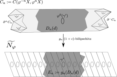
Figure 2. The map from the deep part to the infinite cyclic cover which is shown tessellated by $\phi$-translates of a fundamental domain (depicted as parallograms) each containing a closed geodesic $\varphi^{k}(\gamma^{\prime})$.

Choose a homotopy class $\gamma_{*}$ of a simple closed curve on $X$, and denote the geodesic representative of $\varphi^{k}(\gamma)_{*}$ in $C_{n}$ by $\varphi^{k}(\gamma)$. In particular, there is a collection of $2n+1$ closed geodesics in $C_{n}$,

$$\Gamma_{n}:=\{\varphi^{k}(\gamma)\,:\,-n\leq k\leq n\}.$$

By Minsky [16] the lengths of the geodesics in $\Gamma_{n}$ are uniformly bounded (i.e. not depending on $n$) from above by some $L>0$.

Consider the subset of geodesics belonging to $\Gamma_{n}$ that are not contained in the deep part $D_{n}(d)$, or equivalently, the values of $k$ such that $d(\partial C_{n},\varphi^{k}(\gamma))<d$. By (4.2) one has the inequality

$$\frac{1}{E}(n-|k|)\,{\rm ent}\,\varphi-F_{1}\leq d(\partial C_{n},\varphi^{k}(\gamma))<d$$ (4.5)

for $F_{1}>0$ and $E>1$ which do not depend on $n$. One can explicitly compute $A_{1}>0$ depending on the depth $d$, $\varphi$ and $X$ (but not on $n$) such that the number of values of $k$ which satisfy this inequality, hence the number of curves in $\Gamma_{n}$ not contained in $D_{n}(d)$, is less than $A_{1}$.

Thus the deep part $D_{n}(d)$ contains at least $2n+1-A_{1}$ members of $\Gamma_{n}$ and the image $E_{n}$ contains the same number of $g_{n}(\varphi^{k}(\gamma))$. Our objective is to “promote” each of these latter curves to a fundamental domain for the action of $\varphi$ by translation on $\widetilde{N}_{\varphi}$ contained in $E_{n}$. The curve $g_{n}(\gamma)$ is homotopic to a closed geodesic $\gamma^{\prime}\subset\widetilde{N}_{\varphi}$. Since the length of $\gamma^{\prime}$ is bounded below ($N_{\varphi}$ is compact) and the length of $g_{n}(\gamma)$ uniformly bounded above, by the Morse Lemma stated in point (1) above, the curve $g_{n}(\gamma)$ is contained in an $R$-neighborhood of $\gamma^{\prime}$. It follows that there exists $A_{2}\geq A_{1}$ such that if $n-|k|>A_{2}$ then $\varphi^{k}(\gamma)$ and $g_{n}^{-1}(\varphi^{k}(\gamma^{\prime}))$ are contained in $D_{n}(d)$.

Now define

$$\Delta:=\{x,d(x,\gamma^{\prime})\leq d(x,\varphi^{\pm 1}(\gamma^{\prime})\}\subset\widetilde{N}_{\varphi}.$$ (4.6)

Clearly, the interior of $\Delta$ is a fundamental domain for the action of $\varphi$ on $\widetilde{N}_{\varphi}$ and the diameter of $\Delta$ is bounded since $N_{\varphi}$ is compact. Moreover,

$$d(\partial C_{n},\varphi^{k}(\gamma))$$

$$\quad\leq d(\partial C_{n},g_{n}^{-1}(\varphi^{k}(\Delta)\cap E_{n}))+\text{diam}\,g_{n}^{-1}(\varphi^{k}(\Delta)\cap E_{n})+d(g_{n}^{-1}(\varphi^{k}(\gamma^{\prime})),\varphi^{k}(\gamma)).$$

So that, if $g_{n}^{-1}(\varphi^{k}(\gamma))\subset D_{n}(d)$ then

$$d(\partial C_{n},g_{n}^{-1}(\varphi^{k}(\Delta)\cap E_{n}))$$

$$\qquad\quad\geq d(\partial C_{n},\varphi^{k}(\gamma))-(1+\epsilon)\text{diam}\Delta-d(g_{n}^{-1}(\varphi^{k}(\gamma^{\prime})),\varphi^{k}(\gamma))$$

$$\qquad\quad\geq d(\partial C_{n},\varphi^{k}(\gamma))-(1+\epsilon)\,(\text{diam}\Delta+R).$$

where $\epsilon=\epsilon(D_{n}(d))$. Consequently there exists $A_{3}\geq A_{2}$ such that if $n-|k|\geq A_{3}$ then $g_{n}^{-1}(\varphi^{k}(\Delta))\subset D_{n}(d)$, that is,

$$\bigcup_{|k|<n-A_{3}}g_{n}^{-1}(\varphi^{k}(\Delta))\subset D_{n}(d).$$ (4.7)

From the above estimate one also obtains an explicit “linear” lower bound for the depth by using the information contained in Minsky’s model, $g_{n}^{-1}(\varphi^{k}(\Delta)\cap E_{n})$,

$$d(\partial C_{n},g_{n}^{-1}(\varphi^{k}(\Delta)\cap E_{n}))\geq\frac{1}{E}\,(n-|k|){\rm ent}\,\varphi-F_{1}.$$ (4.8)

The inclusion (4.7) yields a lower bound for the volume as follows

$${\rm vol}\,D_{n}(d) \geq\sum_{|k|\leq n-A_{3}}{\rm vol}\,g_{n}^{-1}(\varphi^{k}(\Delta))$$

$$\geq\sum_{|k|\leq n-A_{3}}(1+\epsilon(g_{n}^{-1}(\varphi^{k}(\Delta)))^{-3}{\rm vol}\,\varphi^{k}(\Delta)$$

$$\geq\sum_{|k|\leq n-A_{3}}(1-4\epsilon(g_{n}^{-1}(\varphi^{k}(\Delta))){\rm vol}\,\varphi^{k}(\Delta)$$

$$\geq 2(n-A_{3}){\rm vol}\,\Delta-4({\rm vol}\,\Delta)\sum_{|k|\leq n-A_{3}}\epsilon(g_{n}^{-1}(\varphi^{k}(\Delta)))$$

The first term is the sum of $2n{\rm vol}\,\Delta$ plus a quantity which does not depend on $n$ and, by (4.8), the second is bounded above by the sum of a geometric series.

In order to bound the volume from above we cover the convex core by two sets. Define,

$$\begin{array}[]{rcl}V_{n}&:=&\bigcup_{|k|\leq n-A_{3}}g_{n}^{-1}(\varphi^{k}(\overline{\Delta}))\\ &&\\ S_{n}&:=&g_{n}^{-1}(\varphi^{-n+A_{3}}(\Delta))\cup g_{n}^{-1}(\varphi^{n-A_{3}}(\Delta)).\end{array}$$

so that one obtains the convex core as the union $V_{n}\cup(S_{n}\cup(C_{n}\setminus V_{n}))$. Observe that $\Delta$ separates $N_{\varphi}$ so $S_{n}$ separates $C_{n}$ and the complement of consists of 3 components; one containing $\partial^{+}C_{n}$, another $\partial^{-}C_{n}$ and the remaining component $g^{-1}(\varphi^{k})$ for $k<|n|-A_{3}$. Clearly, the depth of a point contained in the the components that contain the boundary $\partial C_{n}$ is bounded from above by the maximum depth of a point in $S_{n}$. Let us give an explicit upper bound using (4.2). For $x\in g^{-1}(\varphi^{k}(\Delta))$ one has

$$d(\partial^{-}C_{n},x)\leq d(\partial^{-}C_{n},\varphi^{k}(\gamma))+d(\varphi^{k}(\gamma),x)\leq E(n-|k|)\,{\rm ent}\,\varphi+F_{1}+R+(1+\epsilon)\text{diam}\,\Delta.$$

So that, setting $k=A_{3}$ in the expression on the right, we obtain the required uniform bound, w(it is easy to see that $g^{-1}(\varphi^{k}(\Delta))$ satisfies the same upper bound). It follows that the complement in the convex core of $V_{n}$ is contained in a $T$-regular neighborhood of the boundary $\partial C_{n}$ that is,

$$C_{n}=N_{T}(\partial C_{n})\,\cup V_{n}.$$

From this we obtain the upper bound for volume

$${\rm vol}\,C_{n}\leq{\rm vol}\,N_{T}(\partial C_{n})+{\rm vol}\,V_{n}.$$

The diameter of each of the components of $N_{T}(\partial C_{n})$ is uniformly bounded bounded (by $T+5\,\text{diam}X$) so the first term is uniformly bounded in $n$ and, by a similar calculation to the above for the lower bound, the second term is seen to be bounded from above by $2n{\rm vol}\,\Delta$ plus a constant. ∎

References

- [1] I. Agol, Ideal triangulations of pseudo-Anosov mapping tori, Contemporary Math., 560 (2011), 1-17.
- [2] L. Bers, Simultaneous uniformization, Bull. Amer. Math. Soc., 66 (1960), 94-97.
- [3] L. Bers, An extremal problem for quasiconformal mappings and a theorem by Thurston, Acta. Math., 141 (1978), 73-98.
- [4] M. Bridgeman, Average bending of convex pleated planes in hyperbolic three-space, Invent. Math., 132 (1998), 381-391.
- [5] J. Brock, Weil-Petersson translation distance and volumes of mapping tori, Communications in Analysis and Geometry, 11 (2003), 987–999.
- [6] J. Brock and K. Bromberg, Geoometric inflexibility and 3-manifolds that fiber over the circle, J. Topol., 4 (2011), 1-38.
- [7] C. Cao and R. Meyerhoff, The orientable cusped hyperbolic 3-manifolds of minimal volume, Invent. Math., 146 (2001), 451–478.
- [8] C. Epstein, Envelopes of horospheres and Weingarten surfaces in hyperbolic 3-spaces, preprint, Princeton Univ., (1984).
- [9] D. B. A. Epstein, A. Marden and V. Markovic, Quasiconformal homeomorphisms and the convex hull boundary, Ann. of Math., 59 (2004), 305-336.
- [10] B. Farb, C. Leininger and D. Margalit, Small dilatation pseudo-Anosovs and 3-manifolds, Adv. Math., 228 (2011), 1466-1502.
- [11] F. Gardiner and N. Lakic, Quasiconformal Teichmüller Theory, Mathematical Surveys and Monographs, Volume 76, Amer. Math. Soc., (2000).
- [12] E. Kin, S. Kojima and M. Takasawa, Entropy versus volume for pseudo-Anosovs, Experimental Math., 18 (2009), 397-407.
- [13] S. Kojima, Entropy, Weil-Petersson translation distance and Gromov norm for surface automorphism, Proc. Amer. Math. Soc., 140 (2012), 3993-4002.
- [14] K. Krasnov and J-M. Schlenker, On the renomalized volume of hyperbolic 3-manifolds, Comm. Math. Phy. 279 (2008), 637-668.
- [15] C. McMullen, Renormalization and 3-manifolds which fiber over the circle, Ann. Math. Study 142 (1996).
- [16] Y. Minsky, Bounded geometry for Kleinian groups, Invent. Math., 146 (2001), 143-192,
- [17] Z. Nehari, The Schwarzian derivative and schlicht functions, Bull. Amer. Math. Soc., 55 (1949), 545-551.
- [18] J-M, Schlenker, The renormalized volume and the volume of the convex core of quasifuchsian manifolds, Math. Res. Lett., 20 (2013), 773-786.
- [19] R. Penner, Bounds on least dilatations, Proc. Amer. Math. Soc., 113 (1991), 443-450.
- [20] K. Rafi A characterization of short curves of a Teichmeuller geodesic, Geometry & Topology Volume 9 (2005) 179???202
- [21] C. Y. Tsai, The asymptotic behavior of least pseudo-Anosov dilatations, Geometry and Topology, 13 (2009), 2253–2278.
- [22] W. Thurston, The geometry and topology of -manifolds, Lecture Notes, Princeton University (1979).
- [23] W. Thurston, On the geometry and dynamics of diffeomorphisms of surfaces, Bulletin of Amer. Math. Society., 19 (1988), 417–431.
- [24] W. Thurston, Hyperbolic structures on 3-manifolds II: Surface groups and 3-manifolds which fiber over the circle, preprint.