Structure Regularization for Structured Prediction: Theories and Experiments

Xu Sun∗†
*MOE Key Laboratory of Computational Linguistics, Peking University
{\dagger}School of Electronics Engineering and Computer Science, Peking University
xusun@pku.edu.cn
Abstract

While there are many studies on weight regularization, the study on structure regularization is rare. Many existing systems on structured prediction focus on increasing the level of structural dependencies within the model. However, this trend could have been misdirected, because our study suggests that complex structures are actually harmful to generalization ability in structured prediction. To control structure-based overfitting, we propose a structure regularization framework via structure decomposition, which decomposes training samples into mini-samples with simpler structures, deriving a model with better generalization power. We show both theoretically and empirically that structure regularization can effectively control overfitting risk and lead to better accuracy. As a by-product, the proposed method can also substantially accelerate the training speed. The method and the theoretical results can apply to general graphical models with arbitrary structures. Experiments on well-known tasks demonstrate that our method can easily beat the benchmark systems on those highly-competitive tasks, achieving state-of-the-art accuracies yet with substantially faster training speed.

1 Introduction

Structured prediction models are popularly used to solve structure dependent problems in a wide variety of application domains including natural language processing, bioinformatics, speech recognition, and computer vision. To solve those problems, many structured prediction methods have been developed, with representative models such as conditional random fields (CRFs), deep neural networks, and structured perceptron models. Recently, in order to more accurately capture structural information, some studies emphasize on intensifying structural dependencies in structured prediction, such as applying long range dependencies among tags and developing long distance features or global features.

We argue that over-emphasis on intensive structural dependencies could be misleading, because our study suggests that complex structures are actually harmful to model accuracy. Indeed, while it is obvious that intensive structural dependencies can effectively incorporate structural information, it is less obvious that intensive structural dependencies have a drawback of increasing the generalization risk. Increasing the generalization risk means the trained model tends to overfit the training data, because more complex structures are easier to suffer from overfitting. Formally, our theoretical analysis reveals why and with what degree the structure complexity lowers the generalization ability of trained models. Since this type of overfitting is caused by structure complexity, it can hardly be solved by ordinary regularization methods such as L2subscript𝐿2L_{2} and L1subscript𝐿1L_{1} regularization schemes, which is only for controlling weight complexity.

To deal with this problem, we propose a simple structure regularization solution based on tag structure decomposition. The proposed method decomposes each training sample into multiple mini-samples with simpler structures, deriving a model with better generalization power. The proposed method is easy to implement, and it has several interesting properties: (1) We show both theoretically and empirically that the proposed method can reduce the overfit risk. (2) Keeping the convexity of the objective function: a convex function with a structure regularizer is still convex. (3) No conflict with the weight regularization: we can apply structure regularization together with weight regularization. (4) Accelerating the convergence rate in training. (5) This method can be used for different types of models, including CRFs [10] and perceptrons [5].

The term structural regularization has been used in prior work for regularizing structures of features. For (typically non-structured) classification problems, there are considerable studies on structure-related regularization, including spectral regularization for modeling feature structures in multi-task learning [1], regularizing feature structures for structural large margin classifiers [30], and many recent studies on structured sparsity. Structure sparsity is studied for a variety of non-structured classification models [15, 6] and structured prediction scenarios [20, 14], via adopting mixed norm regularization [18], Group Lasso [32], posterior regularization [8], and a string of variations [2, 17, 9]. Compared with those prior work, we emphasize that our proposal on tag structure regularization is novel. This is because the term structure in all of the aforementioned work refers to structures of feature space, which is substantially different compared with our proposal on regularizing tag structures (interactions among tags).

There are other related studies, including the studies of [27] and [19] on piecewise/decomposed training methods, and the study of [29] on a “lookahead” learning method. Our work differs from [27, 19, 29] mainly because our work is built on a regularization framework, with arguments and justifications on reducing generalization risk and for better accuracy. Also, our method and the theoretical results can fit general graphical models with arbitrary structures, and the detailed algorithm is quite different. On generalization risk analysis, related studies include [4, 21] on non-structured classification and [28, 13, 12] on structured classification.

To the best of our knowledge, this is the first theoretical result on quantifying the relation between structure complexity and the generalization risk in structured prediction, and this is also the first proposal on structure regularization via regularizing tag-interactions. The contributions of this work111See the code at http://klcl.pku.edu.cn/member/sunxu/code.htm are two-fold:

  • On the methodology side, we propose a general purpose structure regularization framework for structured prediction. We show both theoretically and empirically that the proposed method can effectively reduce the overfitting risk in structured prediction, and that the proposed method also has an interesting by-product of accelerating the rates of convergence in training. The structure regularization method and the theoretical analysis do not make assumptions or constraints based on specific structures. In other words, the method and the theoretical results can apply to graphical models with arbitrary structures, including linear chains, trees, and general graphs.

  • On the application side, for several important natural language processing tasks, including part-of-speech tagging, biomedical entity recognition, and word segmentation, our simple method can easily beat the benchmark systems on those highly-competitive tasks, achieving record-breaking accuracies as well as substantially faster training speed.

2 Structure Regularization

We first describe the proposed structure regularization method, and then give theoretical results on analyzing generalization risk and convergence rates.

2.1 Settings

A graph of observations (even with arbitrary structures) can be indexed and be denoted by using an indexed sequence of observations 𝑶={o1,,on}𝑶subscript𝑜1subscript𝑜𝑛\boldsymbol{O}=\{o_{1},\dots,o_{n}\}. We use the term sample to denote 𝑶={o1,,on}𝑶subscript𝑜1subscript𝑜𝑛\boldsymbol{O}=\{o_{1},\dots,o_{n}\}. For example, in natural language processing, a sample may correspond to a sentence of n𝑛n words with dependencies of linear chain structures (e.g., in part-of-speech tagging) or tree structures (e.g., in syntactic parsing). In signal processing, a sample may correspond to a sequence of n𝑛n signals with dependencies of arbitrary structures. For simplicity in analysis, we assume all samples have n𝑛n observations (thus n𝑛n tags). In a typical setting of structured prediction, all the n𝑛n tags have inter-dependencies via connecting each Markov dependency between neighboring tags. Thus, we call n𝑛n as tag structure complexity or simply structure complexity below.

A sample is converted to an indexed sequence of feature vectors 𝒙={𝒙(1),,𝒙(n)}𝒙subscript𝒙1subscript𝒙𝑛\boldsymbol{x}=\{\boldsymbol{x}_{(1)},\dots,\boldsymbol{x}_{(n)}\}, where 𝒙(k)𝒳subscript𝒙𝑘𝒳\boldsymbol{x}_{(k)}\in\mathcal{X} is of the dimension d𝑑d and corresponds to the local features extracted from the position/index k𝑘k.222In most of the existing structured prediction methods, including conditional random fields (CRFs), all the local feature vectors should have the same dimension of features. We can use an n×d𝑛𝑑n\times d matrix to represent 𝒙𝒳n𝒙superscript𝒳𝑛\boldsymbol{x}\in\mathcal{X}^{n}. In other words, we use 𝒳𝒳\mathcal{X} to denote the input space on a position, so that 𝒙𝒙\boldsymbol{x} is sampled from 𝒳nsuperscript𝒳𝑛\mathcal{X}^{n}. Let 𝒴nnsuperscript𝒴𝑛superscript𝑛\mathcal{Y}^{n}\subset\mathbb{R}^{n} be structured output space, so that the structured output 𝒚𝒚\boldsymbol{y} are sampled from 𝒴nsuperscript𝒴𝑛\mathcal{Y}^{n}. Let 𝒵=(𝒳n,𝒴n)𝒵superscript𝒳𝑛superscript𝒴𝑛\mathcal{Z}=(\mathcal{X}^{n},\mathcal{Y}^{n}) be a unified denotation of structured input and output space. Let 𝒛=(𝒙,𝒚)𝒛𝒙𝒚\boldsymbol{z}=(\boldsymbol{x},\boldsymbol{y}), which is sampled from 𝒵𝒵\mathcal{Z}, be a unified denotation of a (𝒙,𝒚)𝒙𝒚(\boldsymbol{x},\boldsymbol{y}) pair in the training data.

Suppose a training set is

S={𝒛1=(𝒙1,𝒚1),,𝒛m=(𝒙m,𝒚m)},𝑆formulae-sequencesubscript𝒛1subscript𝒙1subscript𝒚1subscript𝒛𝑚subscript𝒙𝑚subscript𝒚𝑚S=\{\boldsymbol{z}_{1}=(\boldsymbol{x}_{1},\boldsymbol{y}_{1}),\dots,\boldsymbol{z}_{m}=(\boldsymbol{x}_{m},\boldsymbol{y}_{m})\},

with size m𝑚m, and the samples are drawn i.i.d. from a distribution D𝐷D which is unknown. A learning algorithm is a function G:𝒵m:𝐺maps-tosuperscript𝒵𝑚G:\mathcal{Z}^{m}\mapsto\mathcal{F} with the function space {𝒳n𝒴n}maps-tosuperscript𝒳𝑛superscript𝒴𝑛\mathcal{F}\subset\{\mathcal{X}^{n}\mapsto\mathcal{Y}^{n}\}, i.e., G𝐺G maps a training set S𝑆S to a function GS:𝒳n𝒴n:subscript𝐺𝑆maps-tosuperscript𝒳𝑛superscript𝒴𝑛G_{S}:\mathcal{X}^{n}\mapsto\mathcal{Y}^{n}. We suppose G𝐺G is symmetric with respect to S𝑆S, so that G𝐺G is independent on the order of S𝑆S.

Structural dependencies among tags are the major difference between structured prediction and non-structured classification. For the latter case, a local classification of g𝑔g based on a position k𝑘k can be expressed as g(𝒙(ka),,𝒙(k+a))𝑔subscript𝒙𝑘𝑎subscript𝒙𝑘𝑎g(\boldsymbol{x}_{(k-a)},\dots,\boldsymbol{x}_{(k+a)}), where the term {𝒙(ka),,𝒙(k+a)}subscript𝒙𝑘𝑎subscript𝒙𝑘𝑎\{\boldsymbol{x}_{(k-a)},\dots,\boldsymbol{x}_{(k+a)}\} represents a local window. However, for structured prediction, a local classification on a position depends on the whole input 𝒙={𝒙(1),,𝒙(n)}𝒙subscript𝒙1subscript𝒙𝑛\boldsymbol{x}=\{\boldsymbol{x}_{(1)},\dots,\boldsymbol{x}_{(n)}\} rather than a local window, due to the nature of structural dependencies among tags (e.g., graphical models like CRFs). Thus, in structured prediction a local classification on k𝑘k should be denoted as g(𝒙(1),,𝒙(n),k)𝑔subscript𝒙1subscript𝒙𝑛𝑘g(\boldsymbol{x}_{(1)},\dots,\boldsymbol{x}_{(n)},k). To simplify the notation, we define

g(𝒙,k)g(𝒙(1),,𝒙(n),k)𝑔𝒙𝑘𝑔subscript𝒙1subscript𝒙𝑛𝑘g(\boldsymbol{x},k)\triangleq g(\boldsymbol{x}_{(1)},\dots,\boldsymbol{x}_{(n)},k)

Given a training set S𝑆S of size m𝑚m, we define Sisuperscript𝑆𝑖S^{\setminus i} as a modified training set, which removes the i𝑖i’th training sample:

Si={𝒛1,,𝒛i1,𝒛i+1,,𝒛m},superscript𝑆𝑖subscript𝒛1subscript𝒛𝑖1subscript𝒛𝑖1subscript𝒛𝑚S^{\setminus i}=\{\boldsymbol{z}_{1},\dots,\boldsymbol{z}_{i-1},\boldsymbol{z}_{i+1},\dots,\boldsymbol{z}_{m}\},

and we define Sisuperscript𝑆𝑖S^{i} as another modified training set, which replaces the i𝑖i’th training sample with a new sample 𝒛^isubscriptbold-^𝒛𝑖\boldsymbol{\hat{z}}_{i} drawn from D𝐷D:

Si={𝒛1,,𝒛i1,𝒛^i,𝒛i+1,,𝒛m},superscript𝑆𝑖subscript𝒛1subscript𝒛𝑖1subscriptbold-^𝒛𝑖subscript𝒛𝑖1subscript𝒛𝑚S^{i}=\{\boldsymbol{z}_{1},\dots,\boldsymbol{z}_{i-1},\boldsymbol{\hat{z}}_{i},\boldsymbol{z}_{i+1},\dots,\boldsymbol{z}_{m}\},

We define point-wise cost function c:𝒴×𝒴+:𝑐maps-to𝒴𝒴superscriptc:\mathcal{Y}\times\mathcal{Y}\mapsto\mathbb{R}^{+} as c[GS(𝒙,k),𝒚(k)]𝑐subscript𝐺𝑆𝒙𝑘subscript𝒚𝑘c[G_{S}(\boldsymbol{x},k),\boldsymbol{y}_{(k)}], which measures the cost on a position k𝑘k by comparing GS(𝒙,k)subscript𝐺𝑆𝒙𝑘G_{S}(\boldsymbol{x},k) and the gold-standard tag 𝒚(k)subscript𝒚𝑘\boldsymbol{y}_{(k)}, and we introduce the point-wise loss as

(GS,𝒛,k)c[GS(𝒙,k),𝒚(k)]subscript𝐺𝑆𝒛𝑘𝑐subscript𝐺𝑆𝒙𝑘subscript𝒚𝑘\ell(G_{S},\boldsymbol{z},k)\triangleq c[G_{S}(\boldsymbol{x},k),\boldsymbol{y}_{(k)}]

Then, we define sample-wise cost function C:𝒴n×𝒴n+:𝐶maps-tosuperscript𝒴𝑛superscript𝒴𝑛superscriptC:\mathcal{Y}^{n}\times\mathcal{Y}^{n}\mapsto\mathbb{R}^{+}, which is the cost function with respect to a whole sample, and we introduce the sample-wise loss as

(GS,𝒛)C[GS(𝒙),𝒚]=k=1n(GS,𝒛,k)=k=1nc[GS(𝒙,k),𝒚(k)]subscript𝐺𝑆𝒛𝐶subscript𝐺𝑆𝒙𝒚superscriptsubscript𝑘1𝑛subscript𝐺𝑆𝒛𝑘superscriptsubscript𝑘1𝑛𝑐subscript𝐺𝑆𝒙𝑘subscript𝒚𝑘\mathcal{L}(G_{S},\boldsymbol{z})\triangleq C[G_{S}(\boldsymbol{x}),\boldsymbol{y}]=\sum_{k=1}^{n}\ell(G_{S},\boldsymbol{z},k)=\sum_{k=1}^{n}c[G_{S}(\boldsymbol{x},k),\boldsymbol{y}_{(k)}]

Given G𝐺G and a training set S𝑆S, what we are most interested in is the generalization risk in structured prediction (i.e., expected average loss) [28, 13]:

R(GS)=𝔼𝒛[(GS,𝒛)n]𝑅subscript𝐺𝑆subscript𝔼𝒛delimited-[]subscript𝐺𝑆𝒛𝑛R(G_{S})=\mathbb{E}_{\boldsymbol{z}}\Big{[}\frac{\mathcal{L}(G_{S},\boldsymbol{z})}{n}\Big{]}

Unless specifically indicated in the context, the probabilities and expectations over random variables, including 𝔼𝒛(.)\mathbb{E}_{\boldsymbol{z}}(.), 𝔼S(.)\mathbb{E}_{S}(.), 𝒛(.)\mathbb{P}_{\boldsymbol{z}}(.), and S(.)\mathbb{P}_{S}(.), are based on the unknown distribution D𝐷D.

Since the distribution D𝐷D is unknown, we have to estimate R(GS)𝑅subscript𝐺𝑆R(G_{S}) from S𝑆S by using the empirical risk:

Re(GS)=1mni=1m(GS,𝒛i)=1mni=1mk=1n(GS,𝒛i,k)subscript𝑅𝑒subscript𝐺𝑆1𝑚𝑛superscriptsubscript𝑖1𝑚subscript𝐺𝑆subscript𝒛𝑖1𝑚𝑛superscriptsubscript𝑖1𝑚superscriptsubscript𝑘1𝑛subscript𝐺𝑆subscript𝒛𝑖𝑘R_{e}(G_{S})=\frac{1}{mn}\sum_{i=1}^{m}\mathcal{L}(G_{S},\boldsymbol{z}_{i})=\frac{1}{mn}\sum_{i=1}^{m}\sum_{k=1}^{n}\ell(G_{S},\boldsymbol{z}_{i},k)

In what follows, sometimes we will use simplified notations, R𝑅R and Resubscript𝑅𝑒R_{e}, to denote R(GS)𝑅subscript𝐺𝑆R(G_{S}) and Re(GS)subscript𝑅𝑒subscript𝐺𝑆R_{e}(G_{S}).

To state our theoretical results, we must describe several quantities and assumptions which are important in structured prediction. We follow some notations and assumptions on non-structured classification [4, 21]. We assume a simple real-valued structured prediction scheme such that the class predicted on position k𝑘k of 𝒙𝒙\boldsymbol{x} is the sign of GS(𝒙,k)𝒟subscript𝐺𝑆𝒙𝑘𝒟G_{S}(\boldsymbol{x},k)\in\mathcal{D}.333In practice, many popular structured prediction models have a convex and real-valued cost function (e.g., CRFs). Also, we assume the point-wise cost function cτsubscript𝑐𝜏c_{\tau} is convex and τ𝜏\tau-smooth such that y1,y2𝒟,y𝒴formulae-sequencefor-allsubscript𝑦1subscript𝑦2𝒟for-allsuperscript𝑦𝒴\forall y_{1},y_{2}\in\mathcal{D},\forall y^{*}\in\mathcal{Y}

|cτ(y1,y)cτ(y2,y)|τ|y1y2|subscript𝑐𝜏subscript𝑦1superscript𝑦subscript𝑐𝜏subscript𝑦2superscript𝑦𝜏subscript𝑦1subscript𝑦2|c_{\tau}(y_{1},y^{*})-c_{\tau}(y_{2},y^{*})|\leq\tau|y_{1}-y_{2}| (1)

Then, τ𝜏\tau-smooth versions of the loss and the cost function can be derived according to their prior definitions:

τ(GS,𝒛)=Cτ[GS(𝒙),𝒚]=k=1nτ(GS,𝒛,k)=k=1ncτ[GS(𝒙,k),𝒚(k)]subscript𝜏subscript𝐺𝑆𝒛subscript𝐶𝜏subscript𝐺𝑆𝒙𝒚superscriptsubscript𝑘1𝑛subscript𝜏subscript𝐺𝑆𝒛𝑘superscriptsubscript𝑘1𝑛subscript𝑐𝜏subscript𝐺𝑆𝒙𝑘subscript𝒚𝑘\mathcal{L}_{\tau}(G_{S},\boldsymbol{z})=C_{\tau}[G_{S}(\boldsymbol{x}),\boldsymbol{y}]=\sum_{k=1}^{n}\ell_{\tau}(G_{S},\boldsymbol{z},k)=\sum_{k=1}^{n}c_{\tau}[G_{S}(\boldsymbol{x},k),\boldsymbol{y}_{(k)}]

Also, we use a value ρ𝜌\rho to quantify the bound of |GS(𝒙,k)GSi(𝒙,k)|subscript𝐺𝑆𝒙𝑘subscript𝐺superscript𝑆𝑖𝒙𝑘|G_{S}(\boldsymbol{x},k)-G_{S^{\setminus i}}(\boldsymbol{x},k)| while changing a single sample (with size nnsuperscript𝑛𝑛n^{\prime}\leq n) in the training set with respect to the structured input 𝒙𝒙\boldsymbol{x}. This ρ𝜌\rho-admissible assumption can be formulated as kfor-all𝑘\forall k,

|GS(𝒙,k)GSi(𝒙,k)|ρGSGSi2𝒙2subscript𝐺𝑆𝒙𝑘subscript𝐺superscript𝑆𝑖𝒙𝑘𝜌subscriptnormsubscript𝐺𝑆subscript𝐺superscript𝑆𝑖2subscriptnorm𝒙2|G_{S}(\boldsymbol{x},k)-G_{S^{\setminus i}}(\boldsymbol{x},k)|\leq\rho||G_{S}-G_{S^{\setminus i}}||_{2}\cdot||\boldsymbol{x}||_{2} (2)

where ρ+𝜌superscript\rho\in\mathbb{R}^{+} is a value related to the design of algorithm G𝐺G.

2.2 Structure Regularization

Refer to caption
Figure 1: An illustration of structure regularization in simple linear chain case, which decompose a training sample 𝒛𝒛\boldsymbol{z} with structure complexity 6 into three mini-samples with structure complexity 2. Structure regularization can apply to more general graphs with arbitrary dependencies.
Algorithm 1 Training with structure regularization
1:Input: model weights 𝒘𝒘\boldsymbol{w}, training set S𝑆S, structure regularization strength α𝛼\alpha
2:repeat
3:     Ssuperscript𝑆S^{\prime}\leftarrow\emptyset
4:     for i=1m𝑖1𝑚i=1\to m do
5:         Randomly decompose 𝒛iSsubscript𝒛𝑖𝑆\boldsymbol{z}_{i}\in S into mini-samples Nα(𝒛i)={𝒛(i,1),,𝒛(i,α)}subscript𝑁𝛼subscript𝒛𝑖subscript𝒛𝑖1subscript𝒛𝑖𝛼N_{\alpha}(\boldsymbol{z}_{i})=\{\boldsymbol{z}_{(i,1)},\dots,\boldsymbol{z}_{(i,\alpha)}\}
6:         SSNα(𝒛i)superscript𝑆superscript𝑆subscript𝑁𝛼subscript𝒛𝑖S^{\prime}\leftarrow S^{\prime}\cup N_{\alpha}(\boldsymbol{z}_{i})
7:     end for
8:     for i=1|S|𝑖1superscript𝑆i=1\to|S^{\prime}| do
9:         Sample 𝒛superscript𝒛\boldsymbol{z}^{\prime} uniformly at random from Ssuperscript𝑆S^{\prime}, with gradient g𝒛(𝒘)subscript𝑔superscript𝒛𝒘\nabla g_{\boldsymbol{z}^{\prime}}(\boldsymbol{w})
10:         𝒘𝒘ηg𝒛(𝒘)𝒘𝒘𝜂subscript𝑔superscript𝒛𝒘\boldsymbol{w}\leftarrow\boldsymbol{w}-\eta\nabla g_{\boldsymbol{z}^{\prime}}(\boldsymbol{w})
11:     end for
12:until Convergence
13:return 𝒘𝒘\boldsymbol{w}

Most existing regularization techniques are for regularizing model weights/parameters (e.g., a representative regularizer is the Gaussian regularizer or so called L2subscript𝐿2L_{2} regularizer), and we call such regularization techniques as weight regularization.

Definition 1 (Weight regularization)

Let Nλ:+:subscript𝑁𝜆maps-tosuperscriptN_{\lambda}:\mathcal{F}\mapsto\mathbb{R}^{+} be a weight regularization function on \mathcal{F} with regularization strength λ𝜆\lambda, the structured classification based objective function with general weight regularization is as follows:

Rλ(GS)Re(GS)+Nλ(GS)subscript𝑅𝜆subscript𝐺𝑆subscript𝑅𝑒subscript𝐺𝑆subscript𝑁𝜆subscript𝐺𝑆R_{\lambda}(G_{S})\triangleq R_{e}(G_{S})+N_{\lambda}(G_{S}) (3)

While weight regularization is normalizing model weights, the proposed structure regularization method is normalizing the structural complexity of the training samples. As illustrated in Figure 1, our proposal is based on tag structure decomposition, which can be formally defined as follows:

Definition 2 (Structure regularization)

Let Nα::subscript𝑁𝛼maps-toN_{\alpha}:\mathcal{F}\mapsto\mathcal{F} be a structure regularization function on \mathcal{F} with regularization strength α𝛼\alpha with 1αn1𝛼𝑛1\leq\alpha\leq n, the structured classification based objective function with structure regularization is as follows444The notation N𝑁N is overloaded here. For clarity throughout, N𝑁N with subscript λ𝜆\lambda refers to weight regularization function, and N𝑁N with subscript α𝛼\alpha refers to structure regularization function.:

Rα(GS)Re[GNα(S)]=1mni=1mj=1α[GS,𝒛(i,j)]=1mni=1mj=1αk=1n/α[GS,𝒛(i,j),k]subscript𝑅𝛼subscript𝐺𝑆subscript𝑅𝑒delimited-[]subscript𝐺subscript𝑁𝛼𝑆1𝑚𝑛superscriptsubscript𝑖1𝑚superscriptsubscript𝑗1𝛼subscript𝐺superscript𝑆subscript𝒛𝑖𝑗1𝑚𝑛superscriptsubscript𝑖1𝑚superscriptsubscript𝑗1𝛼superscriptsubscript𝑘1𝑛𝛼subscript𝐺superscript𝑆subscript𝒛𝑖𝑗𝑘R_{\alpha}(G_{S})\triangleq R_{e}[G_{N_{\alpha}(S)}]=\frac{1}{mn}\sum_{i=1}^{m}\sum_{j=1}^{\alpha}\mathcal{L}[G_{S^{\prime}},\boldsymbol{z}_{(i,j)}]=\frac{1}{mn}\sum_{i=1}^{m}\sum_{j=1}^{\alpha}\sum_{k=1}^{n/\alpha}\mathcal{\ell}[G_{S^{\prime}},\boldsymbol{z}_{(i,j)},k] (4)

where Nα(𝐳i)subscript𝑁𝛼subscript𝐳𝑖N_{\alpha}(\boldsymbol{z}_{i}) randomly splits 𝐳isubscript𝐳𝑖\boldsymbol{z}_{i} into α𝛼\alpha mini-samples {𝐳(i,1),,𝐳(i,α)}subscript𝐳𝑖1subscript𝐳𝑖𝛼\{\boldsymbol{z}_{(i,1)},\dots,\boldsymbol{z}_{(i,\alpha)}\}, so that the mini-samples have a distribution on their sizes (structure complexities) with the expected value n=n/αsuperscript𝑛𝑛𝛼n^{\prime}=n/\alpha. Thus, we get

S={𝒛(1,1),z(1,2),,𝒛(1,α)α,,𝒛(m,1),𝒛(m,2),,𝒛(m,α)α}superscript𝑆subscriptsubscript𝒛11subscript𝑧12subscript𝒛1𝛼𝛼subscriptsubscript𝒛𝑚1subscript𝒛𝑚2subscript𝒛𝑚𝛼𝛼S^{\prime}=\{\underbrace{\boldsymbol{z}_{(1,1)},z_{(1,2)},\dots,\boldsymbol{z}_{(1,\alpha)}}_{\alpha},\dots,\underbrace{\boldsymbol{z}_{(m,1)},\boldsymbol{z}_{(m,2)},\dots,\boldsymbol{z}_{(m,\alpha)}}_{\alpha}\} (5)

with mα𝑚𝛼m\alpha mini-samples with expected structure complexity n/α𝑛𝛼n/\alpha. We can denote Ssuperscript𝑆S^{\prime} more compactly as S={𝐳1,𝐳2,,𝐳mα}superscript𝑆superscriptsubscript𝐳1superscriptsubscript𝐳2superscriptsubscript𝐳𝑚𝛼S^{\prime}=\{\boldsymbol{z}_{1}^{\prime},\boldsymbol{z}_{2}^{\prime},\dots,\boldsymbol{z}_{m\alpha}^{\prime}\} and Rα(GS)subscript𝑅𝛼subscript𝐺𝑆R_{\alpha}(G_{S}) can be simplified as

Rα(GS)1mni=1mα(GS,𝒛i)=1mni=1mαk=1n/α[GS,𝒛i,k]subscript𝑅𝛼subscript𝐺𝑆1𝑚𝑛superscriptsubscript𝑖1𝑚𝛼subscript𝐺superscript𝑆superscriptsubscript𝒛𝑖1𝑚𝑛superscriptsubscript𝑖1𝑚𝛼superscriptsubscript𝑘1𝑛𝛼subscript𝐺superscript𝑆superscriptsubscript𝒛𝑖𝑘R_{\alpha}(G_{S})\triangleq\frac{1}{mn}\sum_{i=1}^{m\alpha}\mathcal{L}(G_{S^{\prime}},\boldsymbol{z}_{i}^{\prime})=\frac{1}{mn}\sum_{i=1}^{m\alpha}\sum_{k=1}^{n/\alpha}\mathcal{\ell}[G_{S^{\prime}},\boldsymbol{z}_{i}^{\prime},k] (6)

Note that, when the structure regularization strength α=1𝛼1\alpha=1, we have S=Ssuperscript𝑆𝑆S^{\prime}=S and Rα=Resubscript𝑅𝛼subscript𝑅𝑒R_{\alpha}=R_{e}. The structure regularization algorithm (with the stochastic gradient descent setting) is summarized in Algorithm 1.

Since we know 𝒛=(𝒙,𝒚)𝒛𝒙𝒚\boldsymbol{z}=(\boldsymbol{x},\boldsymbol{y}), the decomposition of 𝒛𝒛\boldsymbol{z} simply means the decomposition of 𝒙𝒙\boldsymbol{x} and 𝒚𝒚\boldsymbol{y}. Recall that 𝒙={𝒙(1),,𝒙(n)}𝒙subscript𝒙1subscript𝒙𝑛\boldsymbol{x}=\{\boldsymbol{x}_{(1)},\dots,\boldsymbol{x}_{(n)}\} is an indexed sequence of the feature vectors, not the observations 𝑶={o1,,on}𝑶subscript𝑜1subscript𝑜𝑛\boldsymbol{O}=\{o_{1},\dots,o_{n}\}. Thus, it should be emphasized that the decomposition of 𝒙𝒙\boldsymbol{x} is the decomposition of the feature vectors, not the original observations. Actually the decomposition of the feature vectors is more convenient and has no information loss — no need to regenerate features. On the other hand, decomposing observations needs to regenerate features and may lose some features.

The structure regularization has no conflict with the weight regularization, and the structure regularization can be applied together with the weight regularization. Actually we will show that applying the structure regularization over the weight regularization can further improve stability and reduce generalization risk.

Definition 3 (Structure & weight regularization)

By combining structure regularization in Definition 2 and weight regularization in Definition 1, the structured classification based objective function is as follows:

Rα,λ(GS)Rα(GS)+Nλ(GS)subscript𝑅𝛼𝜆subscript𝐺𝑆subscript𝑅𝛼subscript𝐺𝑆subscript𝑁𝜆subscript𝐺𝑆R_{\alpha,\lambda}(G_{S})\triangleq R_{\alpha}(G_{S})+N_{\lambda}(G_{S}) (7)

When α=1𝛼1\alpha=1, we have Rα,λ=Re(GS)+Nλ(GS)=Rλsubscript𝑅𝛼𝜆subscript𝑅𝑒subscript𝐺𝑆subscript𝑁𝜆subscript𝐺𝑆subscript𝑅𝜆R_{\alpha,\lambda}=R_{e}(G_{S})+N_{\lambda}(G_{S})=R_{\lambda}.

Like existing weight regularization methods, currently our structure regularization is only for the training stage. Currently we do not use structure regularization in the test stage.

2.3 Stability of Structured Prediction

In contrast to the simplicity of the algorithm, the theoretical analysis is quite technical. First, we analyze the stability of structured prediction.

Definition 4 (Function stability)

A real-valued structured classification algorithm G𝐺G has “function value based stability” (“function stability” for short) ΔΔ\Delta if the following holds: 𝐳=(𝐱,𝐲)𝒵,S𝒵m,i{1,,m},k{1,,n}formulae-sequencefor-all𝐳𝐱𝐲𝒵formulae-sequencefor-all𝑆superscript𝒵𝑚formulae-sequencefor-all𝑖1𝑚for-all𝑘1𝑛\forall\boldsymbol{z}=(\boldsymbol{x},\boldsymbol{y})\in\mathcal{Z},\forall S\in\mathcal{Z}^{m},\forall i\in\{1,\dots,m\},\forall k\in\{1,\dots,n\},

|GS(𝒙,k)GSi(𝒙,k)|Δsubscript𝐺𝑆𝒙𝑘subscript𝐺superscript𝑆𝑖𝒙𝑘Δ|G_{S}(\boldsymbol{x},k)-G_{S^{\setminus i}}(\boldsymbol{x},k)|\leq\Delta
Definition 5 (Loss stability)

A structured classification algorithm G𝐺G has “uniform loss-based stability” (“loss stability” for short) ΔlsubscriptΔ𝑙\Delta_{l} if the following holds: 𝐳𝒵,S𝒵m,i{1,,m},k{1,,n}formulae-sequencefor-all𝐳𝒵formulae-sequencefor-all𝑆superscript𝒵𝑚formulae-sequencefor-all𝑖1𝑚for-all𝑘1𝑛\forall\boldsymbol{z}\in\mathcal{Z},\forall S\in\mathcal{Z}^{m},\forall i\in\{1,\dots,m\},\forall k\in\{1,\dots,n\},

|(GS,𝒛,k)(GSi,𝒛,k)|Δlsubscript𝐺𝑆𝒛𝑘subscript𝐺superscript𝑆𝑖𝒛𝑘subscriptΔ𝑙|\ell(G_{S},\boldsymbol{z},k)-\ell(G_{S^{\setminus i}},\boldsymbol{z},k)|\leq\Delta_{l}

G𝐺G has “sample-wise uniform loss-based stability” (“sample loss stability” for short) ΔssubscriptΔ𝑠\Delta_{s} with respect to the loss function \mathcal{L} if the following holds: 𝐳𝒵,S𝒵m,i{1,,m}formulae-sequencefor-all𝐳𝒵formulae-sequencefor-all𝑆superscript𝒵𝑚for-all𝑖1𝑚\forall\boldsymbol{z}\in\mathcal{Z},\forall S\in\mathcal{Z}^{m},\forall i\in\{1,\dots,m\},

|(GS,𝒛)(GSi,𝒛)|Δssubscript𝐺𝑆𝒛subscript𝐺superscript𝑆𝑖𝒛subscriptΔ𝑠|\mathcal{L}(G_{S},\boldsymbol{z})-\mathcal{L}(G_{S^{\setminus i}},\boldsymbol{z})|\leq\Delta_{s}
Lemma 6 (Loss stability vs. function stability)

If a real-valued structured classification algorithm G𝐺G has function stability ΔΔ\Delta with respect to loss function τsubscript𝜏\ell_{\tau}, then G𝐺G has loss stability

ΔlτΔsubscriptΔ𝑙𝜏Δ\Delta_{l}\leq\tau\Delta

and sample loss stability

ΔsnτΔ.subscriptΔ𝑠𝑛𝜏Δ\Delta_{s}\leq n\tau\Delta.

The proof is in Section 4.

Here, we show that our structure regularizer can further improve stability (thus reduce generalization risk) over a model which already equipped with a weight regularizer.

Theorem 7 (Stability vs. structure regularization)

With a training set S𝑆S of size m𝑚m, let the learning algorithm G𝐺G have the minimizer f𝑓f based on commonly used L2subscript𝐿2L_{2} weight regularization:

f=argmingRα,λ(g)=argming(1mnj=1mατ(g,𝒛j)+λ2g22)𝑓subscriptargmin𝑔subscript𝑅𝛼𝜆𝑔subscriptargmin𝑔1𝑚𝑛superscriptsubscript𝑗1𝑚𝛼subscript𝜏𝑔superscriptsubscript𝒛𝑗𝜆2superscriptsubscriptnorm𝑔22f=\operatornamewithlimits{argmin}_{g\in\mathcal{F}}R_{\alpha,\lambda}(g)=\operatornamewithlimits{argmin}_{g\in\mathcal{F}}\Big{(}\frac{1}{mn}\sum_{j=1}^{m\alpha}\mathcal{L}_{\tau}(g,\boldsymbol{z}_{j}^{\prime})+\frac{\lambda}{2}||g||_{2}^{2}\Big{)} (8)

where α𝛼\alpha denotes structure regularization strength with 1αn1𝛼𝑛1\leq\alpha\leq n.

Also, we have

fi=argmingRα,λi(g)=argming(1mnjiτ(g,𝒛j)+λ2g22)superscript𝑓superscript𝑖subscriptargmin𝑔superscriptsubscript𝑅𝛼𝜆superscript𝑖𝑔subscriptargmin𝑔1𝑚𝑛subscript𝑗superscript𝑖subscript𝜏𝑔superscriptsubscript𝒛𝑗𝜆2superscriptsubscriptnorm𝑔22f^{\setminus{i^{\prime}}}=\operatornamewithlimits{argmin}_{g\in\mathcal{F}}R_{\alpha,\lambda}^{\setminus{i^{\prime}}}(g)=\operatornamewithlimits{argmin}_{g\in\mathcal{F}}\Big{(}\frac{1}{mn}\sum_{j\neq i^{\prime}}\mathcal{L}_{\tau}(g,\boldsymbol{z}_{j}^{\prime})+\frac{\lambda}{2}||g||_{2}^{2}\Big{)} (9)

where ji𝑗superscript𝑖j\neq i^{\prime} means j{1,,i1,i+1,,mα}𝑗1superscript𝑖1superscript𝑖1𝑚𝛼j\in\{1,\dots,i^{\prime}-1,i^{\prime}+1,\dots,m\alpha\}.555Note that, in some cases the notation i𝑖i is ambiguous. For example, fisuperscript𝑓𝑖f^{\setminus i} can either denote the removing of a sample in S𝑆S or denote the removing of a mini-sample in Ssuperscript𝑆S^{\prime}. Thus, when the case is ambiguous, we use different index symbols for S𝑆S and Ssuperscript𝑆S^{\prime}, with i𝑖i for indexing S𝑆S and isuperscript𝑖i^{\prime} for indexing Ssuperscript𝑆S^{\prime}, respectively. Assume τsubscript𝜏\mathcal{L}_{\tau} is convex and differentiable, and f(𝐱,k)𝑓𝐱𝑘f(\boldsymbol{x},k) is ρ𝜌\rho-admissible. Let a local feature value is bounded by v𝑣v such that 𝐱(k,q)vsubscript𝐱𝑘𝑞𝑣\boldsymbol{x}_{(k,q)}\leq v for q{1,,d}𝑞1𝑑q\in\{1,\dots,d\}.666Recall that d𝑑d is the dimension of local feature vectors defined in Section 2.1. Let ΔΔ\Delta denote the function stability of f𝑓f comparing with fisuperscript𝑓superscript𝑖f^{\setminus{i^{\prime}}} for 𝐳𝒵for-all𝐳𝒵\forall\boldsymbol{z}\in\mathcal{Z} with |𝐳|=n𝐳𝑛|\boldsymbol{z}|=n. Then, ΔΔ\Delta is bounded by

Δdτρ2v2n2mλα2,Δ𝑑𝜏superscript𝜌2superscript𝑣2superscript𝑛2𝑚𝜆superscript𝛼2\Delta\leq\frac{d\tau\rho^{2}v^{2}n^{2}}{m\lambda\alpha^{2}}, (10)

and the corresponding loss stability is bounded by

Δldτ2ρ2v2n2mλα2,subscriptΔ𝑙𝑑superscript𝜏2superscript𝜌2superscript𝑣2superscript𝑛2𝑚𝜆superscript𝛼2\Delta_{l}\leq\frac{d\tau^{2}\rho^{2}v^{2}n^{2}}{m\lambda\alpha^{2}},

and the corresponding sample loss stability is bounded by

Δsdτ2ρ2v2n3mλα2.subscriptΔ𝑠𝑑superscript𝜏2superscript𝜌2superscript𝑣2superscript𝑛3𝑚𝜆superscript𝛼2\Delta_{s}\leq\frac{d\tau^{2}\rho^{2}v^{2}n^{3}}{m\lambda\alpha^{2}}.

The proof is in Section 4.

We can see that increasing the size of training set m𝑚m results in linear improvement of ΔΔ\Delta, and increasing the strength of structure regularization α𝛼\alpha results in quadratic improvement of ΔΔ\Delta.

The function stability ΔΔ\Delta is based on comparing f𝑓f and fisuperscript𝑓superscript𝑖f^{\setminus i^{\prime}}, i.e., the stability is based on removing a mini-sample. Moreover, we can extend the analysis to the function stability based on comparing f𝑓f and fisuperscript𝑓𝑖f^{\setminus i}, i.e., the stability is based on removing a full-size sample.

Corollary 8 (Stability based on i𝑖\setminus i rather than isuperscript𝑖\setminus{i^{\prime}})

With a training set S𝑆S of size m𝑚m, let the learning algorithm G𝐺G have the minimizer f𝑓f as defined like before. Also, we have

fi=argmingRα,λi(g)=argming(1mnjiτ(g,𝒛j)+λ2g22)superscript𝑓𝑖subscriptargmin𝑔superscriptsubscript𝑅𝛼𝜆𝑖𝑔subscriptargmin𝑔1𝑚𝑛subscript𝑗𝑖subscript𝜏𝑔superscriptsubscript𝒛𝑗𝜆2superscriptsubscriptnorm𝑔22f^{\setminus{i}}=\operatornamewithlimits{argmin}_{g\in\mathcal{F}}R_{\alpha,\lambda}^{\setminus{i}}(g)=\operatornamewithlimits{argmin}_{g\in\mathcal{F}}\Big{(}\frac{1}{mn}\sum_{j\notin i}\mathcal{L}_{\tau}(g,\boldsymbol{z}_{j}^{\prime})+\frac{\lambda}{2}||g||_{2}^{2}\Big{)} (11)

where ji𝑗𝑖j\notin i means j{1,,(i1)α,iα+1,,mα}𝑗1𝑖1𝛼𝑖𝛼1𝑚𝛼j\in\{1,\dots,(i-1)\alpha,i\alpha+1,\dots,m\alpha\}, i.e., all the mini-samples derived from the sample 𝐳isubscript𝐳𝑖\boldsymbol{z}_{i} are removed. Assume τsubscript𝜏\mathcal{L}_{\tau} is convex and differentiable, and f(𝐱,k)𝑓𝐱𝑘f(\boldsymbol{x},k) is ρ𝜌\rho-admissible. Let a local feature value is bounded by v𝑣v such that 𝐱(k,q)vsubscript𝐱𝑘𝑞𝑣\boldsymbol{x}_{(k,q)}\leq v for q{1,,d}𝑞1𝑑q\in\{1,\dots,d\}. Let Δ¯¯Δ\bar{\Delta} denote the function stability of f𝑓f comparing with fisuperscript𝑓𝑖f^{\setminus i} for 𝐳𝒵for-all𝐳𝒵\forall\boldsymbol{z}\in\mathcal{Z} with |𝐳|=n𝐳𝑛|\boldsymbol{z}|=n. Then, Δ¯¯Δ\bar{\Delta} is bounded by

Δ¯dτρ2v2n2mλα=αsup(Δ),¯Δ𝑑𝜏superscript𝜌2superscript𝑣2superscript𝑛2𝑚𝜆𝛼𝛼supremumΔ\bar{\Delta}\leq\frac{d\tau\rho^{2}v^{2}n^{2}}{m\lambda\alpha}=\alpha\sup(\Delta), (12)

where ΔΔ\Delta is the function stability of f𝑓f comparing with fisuperscript𝑓superscript𝑖f^{\setminus i^{\prime}}, and sup(Δ)=dτρ2v2n2mλα2supremumΔ𝑑𝜏superscript𝜌2superscript𝑣2superscript𝑛2𝑚𝜆superscript𝛼2\sup(\Delta)=\frac{d\tau\rho^{2}v^{2}n^{2}}{m\lambda\alpha^{2}}, as described in Eq. (10). Similarly, we have

Δ¯ldτ2ρ2v2n2mλα=αsup(Δl),subscript¯Δ𝑙𝑑superscript𝜏2superscript𝜌2superscript𝑣2superscript𝑛2𝑚𝜆𝛼𝛼supremumsubscriptΔ𝑙\bar{\Delta}_{l}\leq\frac{d\tau^{2}\rho^{2}v^{2}n^{2}}{m\lambda\alpha}=\alpha\sup(\Delta_{l}),

and

Δ¯sdτ2ρ2v2n3mλα=αsup(Δs).subscript¯Δ𝑠𝑑superscript𝜏2superscript𝜌2superscript𝑣2superscript𝑛3𝑚𝜆𝛼𝛼supremumsubscriptΔ𝑠\bar{\Delta}_{s}\leq\frac{d\tau^{2}\rho^{2}v^{2}n^{3}}{m\lambda\alpha}=\alpha\sup(\Delta_{s}).

The proof is in Section 4.

2.4 Reduction of Generalization Risk

Theorem 9 (Generalization vs. stability)

Let G𝐺G be a real-valued structured classification algorithm with a point-wise loss function τsubscript𝜏\ell_{\tau} such that k,0τ(GS,𝐳,k)γfor-all𝑘0subscript𝜏subscript𝐺𝑆𝐳𝑘𝛾\forall k,0\leq\ell_{\tau}(G_{S},\boldsymbol{z},k)\leq\gamma. Let f𝑓f, ΔΔ\Delta, and Δ¯¯Δ\bar{\Delta} be defined like before. Let R(f)𝑅𝑓R(f) be the generalization risk of f𝑓f based on the expected sample 𝐳𝒵𝐳𝒵\boldsymbol{z}\in\mathcal{Z} with size n𝑛n, as defined like before. Let Re(f)subscript𝑅𝑒𝑓R_{e}(f) be the empirical risk of f𝑓f based on S𝑆S, as defined like before. Then, for any δ(0,1)𝛿01\delta\in(0,1), with probability at least 1δ1𝛿1-\delta over the random draw of the training set S𝑆S, the generalization risk R(f)𝑅𝑓R(f) is bounded by

R(f)Re(f)+2τΔ¯+((4m2)τΔ¯+γ)lnδ12m𝑅𝑓subscript𝑅𝑒𝑓2𝜏¯Δ4𝑚2𝜏¯Δ𝛾superscript𝛿12𝑚R(f)\leq R_{e}(f)+{2\tau\bar{\Delta}}+\Big{(}{(4m-2)\tau\bar{\Delta}}+\gamma\Big{)}\sqrt{\frac{\ln{\delta^{-1}}}{2m}} (13)

The proof is in Section 4.

Theorem 10 (Generalization vs. structure regularization)

Let the structured prediction objective function of G𝐺G be penalized by structure regularization with factor α[1,n]𝛼1𝑛\alpha\in[1,n] and L2subscript𝐿2L_{2} weight regularization with factor λ𝜆\lambda, and the penalized function has a minimizer f𝑓f:

f=argmingRα,λ(g)=argming(1mnj=1mατ(g,𝒛j)+λ2g22)𝑓subscriptargmin𝑔subscript𝑅𝛼𝜆𝑔subscriptargmin𝑔1𝑚𝑛superscriptsubscript𝑗1𝑚𝛼subscript𝜏𝑔superscriptsubscript𝒛𝑗𝜆2superscriptsubscriptnorm𝑔22f=\operatornamewithlimits{argmin}_{g\in\mathcal{F}}R_{\alpha,\lambda}(g)=\operatornamewithlimits{argmin}_{g\in\mathcal{F}}\Big{(}\frac{1}{mn}\sum_{j=1}^{m\alpha}\mathcal{L}_{\tau}(g,\boldsymbol{z}_{j}^{\prime})+\frac{\lambda}{2}||g||_{2}^{2}\Big{)} (14)

Assume the point-wise loss τsubscript𝜏\ell_{\tau} is convex and differentiable, and is bounded by τ(f,𝐳,k)γsubscript𝜏𝑓𝐳𝑘𝛾\ell_{\tau}(f,\boldsymbol{z},k)\leq\gamma. Assume f(𝐱,k)𝑓𝐱𝑘f(\boldsymbol{x},k) is ρ𝜌\rho-admissible. Let a local feature value be bounded by v𝑣v such that 𝐱(k,q)vsubscript𝐱𝑘𝑞𝑣\boldsymbol{x}_{(k,q)}\leq v for q{1,,d}𝑞1𝑑q\in\{1,\dots,d\}. Then, for any δ(0,1)𝛿01\delta\in(0,1), with probability at least 1δ1𝛿1-\delta over the random draw of the training set S𝑆S, the generalization risk R(f)𝑅𝑓R(f) is bounded by

R(f)Re(f)+2dτ2ρ2v2n2mλα+((4m2)dτ2ρ2v2n2mλα+γ)lnδ12m𝑅𝑓subscript𝑅𝑒𝑓2𝑑superscript𝜏2superscript𝜌2superscript𝑣2superscript𝑛2𝑚𝜆𝛼4𝑚2𝑑superscript𝜏2superscript𝜌2superscript𝑣2superscript𝑛2𝑚𝜆𝛼𝛾superscript𝛿12𝑚R(f)\leq R_{e}(f)+{\frac{2d\tau^{2}\rho^{2}v^{2}n^{2}}{m\lambda\alpha}}+\Big{(}{\frac{(4m-2)d\tau^{2}\rho^{2}v^{2}n^{2}}{m\lambda\alpha}}+\gamma\Big{)}\sqrt{\frac{\ln{\delta^{-1}}}{2m}} (15)

The proof is in Section 4.

We call the term 2dτ2ρ2v2n2mλα+((4m2)dτ2ρ2v2n2mλα+γ)lnδ12m2𝑑superscript𝜏2superscript𝜌2superscript𝑣2superscript𝑛2𝑚𝜆𝛼4𝑚2𝑑superscript𝜏2superscript𝜌2superscript𝑣2superscript𝑛2𝑚𝜆𝛼𝛾superscript𝛿12𝑚{\frac{2d\tau^{2}\rho^{2}v^{2}n^{2}}{m\lambda\alpha}}+\Big{(}{\frac{(4m-2)d\tau^{2}\rho^{2}v^{2}n^{2}}{m\lambda\alpha}}+\gamma\Big{)}\sqrt{\frac{\ln{\delta^{-1}}}{2m}} in (15) as “overfit-bound”, and reducing the overfit-bound is crucial for reducing the generalization risk bound. Most importantly, we can see from the overfit-bound that the structure regularization factor α𝛼\alpha is always staying together with the weight regularization factor λ𝜆\lambda, working together on reducing the overfit-bound. This indicates that the structure regularization is as important as the weight regularization for reducing the generalization risk for structured prediction.

Moreover, since τ,ρ𝜏𝜌\tau,\rho, and v𝑣v are typically small compared with other variables, especially m𝑚m, (15) can be approximated as follows by ignoring small terms:

R(f)Re(f)+O(dn2lnδ1λαm)𝑅𝑓subscript𝑅𝑒𝑓𝑂𝑑superscript𝑛2superscript𝛿1𝜆𝛼𝑚R(f)\leq R_{e}(f)+O\Big{(}\frac{dn^{2}\sqrt{\ln{\delta^{-1}}}}{\lambda\alpha\sqrt{m}}\Big{)} (16)

First, (16) suggests that structure complexity n𝑛n can increase the overfit-bound on a magnitude of O(n2)𝑂superscript𝑛2O(n^{2}), and applying weight regularization can reduce the overfit-bound by O(λ)𝑂𝜆O(\lambda). Importantly, applying structure regularization further (over weight regularization) can additionally reduce the overfit-bound by a magnitude of O(α)𝑂𝛼O(\alpha). When α=1𝛼1\alpha=1, it means “no structure regularization”, then we have the worst overfit-bound. Also, (16) suggests that increasing the size of training set can reduce the overfit-bound on a square root level.

Theorem 10 also indicates that too simple structures may overkill the overfit-bound but with a dominating empirical risk, and too complex structures may overkill the empirical risk but with a dominating overfit-bound. Thus, to achieve the best prediction accuracy, a balanced complexity of structures should be used for training the model.

2.5 Accelerating Convergence Rates in Training

We also analyze the impact on the convergence rate of online learning by applying structure regularization. Our analysis is based on the stochastic gradient descent (SGD) setting [3, 11, 16], which is arguably the most representative online training setting. Let g(𝒘)𝑔𝒘g(\boldsymbol{w}) be the structured prediction objective function and 𝒘𝒲𝒘𝒲\boldsymbol{w}\in\mathcal{W} is the weight vector. Recall that the SGD update with fixed learning rate η𝜂\eta has a form like this:

𝒘t+1𝒘tηg𝒛t(𝒘t)subscript𝒘𝑡1subscript𝒘𝑡𝜂subscript𝑔subscript𝒛𝑡subscript𝒘𝑡\boldsymbol{w}_{t+1}\leftarrow\boldsymbol{w}_{t}-\eta\nabla g_{\boldsymbol{z}_{t}}(\boldsymbol{w}_{t}) (17)

where g𝒛(𝒘t)subscript𝑔𝒛subscript𝒘𝑡g_{\boldsymbol{z}}(\boldsymbol{w}_{t}) is the stochastic estimation of the objective function based on 𝒛𝒛\boldsymbol{z} which is randomly drawn from S𝑆S.

To state our convergence rate analysis results, we need several assumptions following (Nemirovski et al. 2009). We assume g𝑔g is strongly convex with modulus c𝑐c, that is, 𝒘,𝒘𝒲for-all𝒘superscript𝒘𝒲\forall\boldsymbol{w},\boldsymbol{w}^{\prime}\in\mathcal{W},

g(𝒘)g(𝒘)+(𝒘𝒘)Tg(𝒘)+c2𝒘𝒘2𝑔superscript𝒘𝑔𝒘superscriptsuperscript𝒘𝒘𝑇𝑔𝒘𝑐2superscriptnormsuperscript𝒘𝒘2g(\boldsymbol{w}^{\prime})\geq g(\boldsymbol{w})+(\boldsymbol{w}^{\prime}-\boldsymbol{w})^{T}\nabla g(\boldsymbol{w})+\frac{c}{2}||\boldsymbol{w}^{\prime}-\boldsymbol{w}||^{2} (18)

When g𝑔g is strongly convex, there is a global optimum/minimizer 𝒘superscript𝒘\boldsymbol{w}^{*}. We also assume Lipschitz continuous differentiability of g𝑔g with the constant q𝑞q, that is, 𝒘,𝒘𝒲for-all𝒘superscript𝒘𝒲\forall\boldsymbol{w},\boldsymbol{w}^{\prime}\in\mathcal{W},

g(𝒘)g(𝒘)q𝒘𝒘norm𝑔superscript𝒘𝑔𝒘𝑞normsuperscript𝒘𝒘||\nabla g(\boldsymbol{w}^{\prime})-\nabla g(\boldsymbol{w})||\leq q||\boldsymbol{w}^{\prime}-\boldsymbol{w}|| (19)

It is also reasonable to assume that the norm of g𝒛(𝒘)subscript𝑔𝒛𝒘\nabla g_{\boldsymbol{z}}(\boldsymbol{w}) has almost surely positive correlation with the structure complexity of 𝒛𝒛\boldsymbol{z},777Many structured prediction systems (e.g., CRFs) satisfy this assumption that the gradient based on a larger sample (i.e., n𝑛n is large) is expected to have a larger norm. which can be quantified by a bound κ+𝜅superscript\kappa\in\mathbb{R}^{+}:

g𝒛(𝒘)2κ|𝒛|almost surely for𝒘𝒲formulae-sequencesubscriptnormsubscript𝑔𝒛𝒘2𝜅𝒛almost surely forfor-all𝒘𝒲||\nabla g_{\boldsymbol{z}}(\boldsymbol{w})||_{2}\leq\kappa|\boldsymbol{z}|\ \ \ \text{almost surely for}\ \ \ \forall\boldsymbol{w}\in\mathcal{W} (20)

where |𝒛|𝒛|\boldsymbol{z}| denotes the structure complexity of 𝒛𝒛\boldsymbol{z}. Moreover, it is reasonable to assume

ηc<1𝜂𝑐1\eta c<1 (21)

because even the ordinary gradient descent methods will diverge if ηc>1𝜂𝑐1\eta c>1.

Then, we show that structure regularization can quadratically accelerate the SGD rates of convergence:

Proposition 11 (Convergence rates vs. structure regularization)

With the aforementioned assumptions, let the SGD training have a learning rate defined as η=cϵβα2qκ2n2𝜂𝑐italic-ϵ𝛽superscript𝛼2𝑞superscript𝜅2superscript𝑛2\eta=\frac{c\epsilon\beta\alpha^{2}}{q\kappa^{2}n^{2}}, where ϵ>0italic-ϵ0\epsilon>0 is a convergence tolerance value and β(0,1]𝛽01\beta\in(0,1]. Let t𝑡t be a integer satisfying

tqκ2n2log(qa0/ϵ)ϵβc2α2𝑡𝑞superscript𝜅2superscript𝑛2𝑞subscript𝑎0italic-ϵitalic-ϵ𝛽superscript𝑐2superscript𝛼2t\geq\frac{q\kappa^{2}n^{2}\log{(qa_{0}/\epsilon)}}{\epsilon\beta c^{2}\alpha^{2}} (22)

where n𝑛n and α[1,n]𝛼1𝑛\alpha\in[1,n] is like before, and a0subscript𝑎0a_{0} is the initial distance which depends on the initialization of the weights 𝐰0subscript𝐰0\boldsymbol{w}_{0} and the minimizer 𝐰superscript𝐰\boldsymbol{w}^{*}, i.e., a0=𝐰0𝐰2subscript𝑎0superscriptnormsubscript𝐰0superscript𝐰2a_{0}=||\boldsymbol{w}_{0}-\boldsymbol{w}^{*}||^{2}. Then, after t𝑡t updates of 𝐰𝐰\boldsymbol{w} it converges to 𝔼[g(𝐰t)g(𝐰)]ϵ𝔼delimited-[]𝑔subscript𝐰𝑡𝑔superscript𝐰italic-ϵ\mathbb{E}[g(\boldsymbol{w}_{t})-g(\boldsymbol{w}^{*})]\leq\epsilon.

The proof is in Section 4.

This Proposition demonstrates the 1/t1𝑡1/t convergence rate with t𝑡t given in (22). Recall that when α=1𝛼1\alpha=1, the algorithm with structure regularization reduces exactly to the ordinary algorithm (without structure regularization), which has the number of SGD updates tqκ2n2log(qa0/ϵ)ϵβc2𝑡𝑞superscript𝜅2superscript𝑛2𝑞subscript𝑎0italic-ϵitalic-ϵ𝛽superscript𝑐2t\geq\frac{q\kappa^{2}n^{2}\log{(qa_{0}/\epsilon)}}{\epsilon\beta c^{2}} to achieve the convergence tolerance value ϵitalic-ϵ\epsilon. In other words, applying structure regularization with the strength α𝛼\alpha can quadratically accelerate the convergence rate with a factor of α2superscript𝛼2\alpha^{2}.

3 Experiments

3.1 Tasks

Diversified Tasks. We experiment on natural language processing tasks and signal processing tasks. The natural language processing tasks include (1) part-of-speech tagging, (2) biomedical named entity recognition, and (3) Chinese word segmentation. The signal processing task is (4) sensor-based human activity recognition. The tasks (1) to (3) use boolean features and the task (4) adopts real-valued features. From tasks (1) to (4), the averaged structure complexity (number of observations) n𝑛n is very different, with n=23.9,26.5,46.6,67.9𝑛23.926.546.667.9n=23.9,26.5,46.6,67.9, respectively. The dimension of tags |𝒴|𝒴|\mathcal{Y}| is also diversified among tasks, with |𝒴|𝒴|\mathcal{Y}| ranging from 5 to 45.

Part-of-Speech Tagging (POS-Tagging). Part-of-Speech (POS) tagging is an important and highly competitive task in natural language processing. We use the standard benchmark dataset in prior work [5], which is derived from PennTreeBank corpus and uses sections 0 to 18 of the Wall Street Journal (WSJ) for training (38,219 samples), and sections 22-24 for testing (5,462 samples). Following prior work [29], we use features based on unigrams and bigrams of neighboring words, and lexical patterns of the current word, with 393,741 raw features888Raw features are those observation features based only on 𝒙𝒙\boldsymbol{x}, i.e., no combination with tag information. in total. Following prior work, the evaluation metric for this task is per-word accuracy.

Biomedical Named Entity Recognition (Bio-NER). This task is from the BioNLP-2004 shared task, which is for recognizing 5 kinds of biomedical named entities (DNA, RNA, etc.) on the MEDLINE biomedical text corpus. There are 17,484 training samples and 3,856 test samples. Following prior work [29], we use word pattern features and POS features, with 403,192 raw features in total. The evaluation metric is balanced F-score.

Word Segmentation (Word-Seg). Chinese word segmentation is important and it is usually the first step for text processing in Chinese. We use the Microsoft Research (MSR) data provided by SIGHAN-2004 contest. There are 86,918 training samples and 3,985 test samples. Following prior work [7], we use features based on character unigrams and bigrams, with 1,985,720 raw features in total. The evaluation metric for this task is balanced F-score.

Sensor-based Human Activity Recognition (Act-Recog). This is a task based on real-valued sensor signals, with the data extracted from the Bao04 activity recognition dataset [24]. This task aims to recognize human activities (walking, bicycling, etc.) by using 5 biaxial sensors to collect acceleration signals of individuals, with the sampling frequency at 76.25HZ. Following prior work in activity recognition [24], we use acceleration features, mean features, standard deviation, energy, and correlation features, with 1228 raw features in total. There are 16,000 training samples and 4,000 test samples. Following prior work, the evaluation metric is accuracy.

3.2 Experimental Settings

To test the robustness of the proposed structure regularization (StructReg) method, we perform experiments on both probabilistic and non-probabilistic structure prediction models. We choose the conditional random fields (CRFs) [10] and structured perceptrons (Perc) [5], which are arguably the most popular probabilistic and non-probabilistic structured prediction models, respectively. The CRFs are trained using the SGD algorithm,999In theoretical analysis, following prior work we adopt the SGD with fixed learning rate, as described in Section 2.5. However, since the SGD with decaying learning rate is more commonly used in practice, in experiments we use the SGD with decaying learning rate. and the baseline method is the traditional weight regularization scheme (WeightReg), which adopts the most representative L2subscript𝐿2L_{2} weight regularization, i.e., a Gaussian prior.101010We also tested on sparsity emphasized regularization methods, including L1subscript𝐿1L_{1} regularization and Group Lasso regularization [14]. However, we find that in most cases those sparsity emphasized regularization methods have lower accuracy than the L2subscript𝐿2L_{2} regularization. For the structured perceptrons, the baseline WeightAvg is the popular implicit regularization technique based on parameter averaging, i.e., averaged perceptron [5].

All methods use the same set of features. Since the rich edge features [26, 25] can be automatically generated from raw features and are very useful for improving model accuracy, the rich edge features are employed for all methods. All methods are based on the 1st-order Markov dependency. For WeightReg, the L2subscript𝐿2L_{2} regularization strengths (i.e., λ/2𝜆2\lambda/2 in Eq.8) are tuned among values 0.1,0.5,1,2,50.10.51250.1,0.5,1,2,5, and are determined on the development data provided by the standard dataset (POS-Tagging) or simply via 4-fold cross validation on the training set (Bio-NER, Word-Seg, and Act-Recog). With this automatic tuning for WeightReg, we set 2,5,12512,5,1 and 555 for POS-Tagging, Bio-NER, Word-Seg, and Act-Recog tasks, respectively. Our StructReg method adopts the same L2subscript𝐿2L_{2} regularization setting like WeightReg. Experiments are performed on a computer with Intel(R) Xeon(R) 3.0GHz CPU.

3.3 Experimental Results
Refer to caption Refer to caption Refer to caption Refer to caption
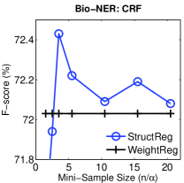
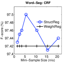
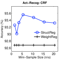
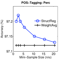
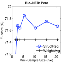
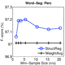
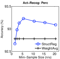
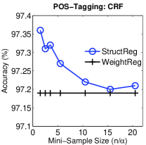
Figure 2: On the four tasks, comparing the structure regularization method (StructReg) with existing regularization methods in terms of accuracy/F-score. Row-1 shows the results on CRFs and Row-2 shows the results on structured perceptrons.
Table 1: Comparing our results with the benchmark systems on corresponding tasks.
POS-Tagging (Acc%) Bio-NER (F1%) Word-Seg (F1%)
Benchmark system 97.33 (see [22]) 72.28 (see [29]) 97.19 (see [7])
Our results 97.36 72.43 97.50
Refer to caption Refer to caption Refer to caption Refer to caption
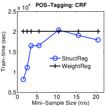
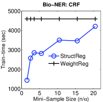
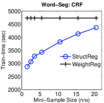
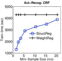
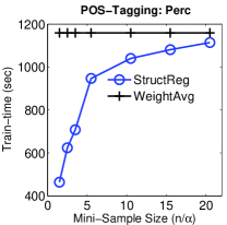
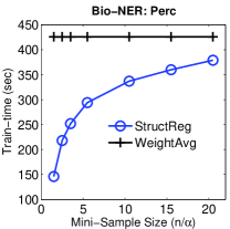
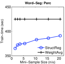
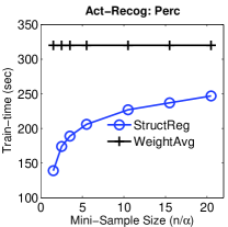
Figure 3: On the four tasks, comparing the structure regularization method (StructReg) with existing regularization methods in terms of wall-clock training time.

The experimental results in terms of accuracy/F-score are shown in Figure 2. For the CRF model, the training is convergent, and the results on the convergence state (decided by relative objective change with the threshold value of 0.00010.00010.0001) are shown. For the structured perceptron model, the training is typically not convergent, and the results on the 10’th iteration are shown. For stability of the curves, the results of the structured perceptrons are averaged over 10 repeated runs.

Since different samples have different size n𝑛n in practice, we set α𝛼\alpha being a function of n𝑛n, so that the generated mini-samples are with fixed size nsuperscript𝑛n^{\prime} with n=n/αsuperscript𝑛𝑛𝛼n^{\prime}=n/\alpha. Actually, nsuperscript𝑛n^{\prime} is a probabilistic distribution because we adopt randomized decomposition. For example, if n=5.5superscript𝑛5.5n^{\prime}=5.5, it means the mini-samples are a mixture of the ones with the size 5 and the ones with the size 6, and the mean of the size distribution is 5.5. In the figure, the curves are based on n=1.5,2.5,3.5,5.5,10.5,15.5,20.5superscript𝑛1.52.53.55.510.515.520.5n^{\prime}=1.5,2.5,3.5,5.5,10.5,15.5,20.5.

As we can see, although the experiments are based on very different models (probabilistic or non-probabilistic), with diversified feature types (boolean or real-value) and different structure complexity n𝑛n, the results are quite consistent. It demonstrates that structure regularization leads to higher accuracies/F-scores compared with the existing baselines.

We also conduct significance tests based on t-test. Since the t-test for F-score based tasks (Bio-NER and Word-Seg) may be unreliable111111Indeed we can convert F-scores to accuracy scores for t-test, but in many cases this conversion is unreliable. For example, very different F-scores may correspond to similar accuracy scores., we only perform t-test for the accuracy-based tasks, i.e., POS-Tagging and Act-Recog. For POS-Tagging, the significance test suggests that the superiority of StructReg over WeightReg is very statistically significant, with p<0.01𝑝0.01p<0.01. For Act-Recog, the significance tests suggest that both the StructReg vs. WeightReg difference and the StructReg vs. WeightAvg difference are extremely statistically significant, with p<0.0001𝑝0.0001p<0.0001 in both cases. The experimental results support our theoretical analysis that structure regularization can further reduce the generalization risk over existing weight regularization techniques.

Our method actually outperforms the benchmark systems on the three important natural language processing tasks. The POS-Tagging task is a highly competitive task, with many methods proposed, and the best report (without using extra resources) until now is achieved by using a bidirectional learning model in [22],121212See a collection of the systems at http://aclweb.org/aclwiki/index.php?title=POS_Tagging_(State_of_the_art) with the accuracy 97.33%. Our simple method achieves better accuracy compared with all of those state-of-the-art systems. Furthermore, our method achieves as good scores as the benchmark systems on the Bio-NER and Word-Seg tasks, which are also very competitive tasks in natural language processing communities. On the Bio-NER task, [29] achieves 72.28% based on lookahead learning and [31] achieves 72.65% based on reranking. On the Word-Seg task, [7] achieves 97.19% based on maximum entropy classification and our recent work [25] achieves 97.5% based on feature-frequency-adaptive online learning. The comparisons are summarized in Table 1. Note that, similar to the tuning on the WeightReg strengths, the optimal values of StructReg strengths are also decided automatically based on standard development data or cross validation on training data.

Figure 3 shows experimental comparisons in terms of wall-clock training time. As we can see, the proposed method can substantially improve the training speed. The speedup is not only from the faster convergence rates, but also from the faster processing time on the structures, because it is more efficient to process the decomposed samples with simple structures.

4 Proofs

Our analysis sometimes need to use McDiarmid’s inequality.

Theorem 12 (McDiarmid, 1989)

Let S={q1,,qm}𝑆subscript𝑞1subscript𝑞𝑚S=\{q_{1},\dots,q_{m}\} be independent random variables taking values in the space Qmsuperscript𝑄𝑚Q^{m}. Moreover, let g:Qm:𝑔maps-tosuperscript𝑄𝑚g:Q^{m}\mapsto\mathbb{R} be a function of S𝑆S that satisfies i,SQm,q^iQ,formulae-sequencefor-all𝑖for-all𝑆superscript𝑄𝑚for-allsubscript^𝑞𝑖𝑄\forall i,\forall S\in Q^{m},\forall\hat{q}_{i}\in Q,

|g(S)g(Si)|ci.𝑔𝑆𝑔superscript𝑆𝑖subscript𝑐𝑖|g(S)-g(S^{i})|\leq c_{i}.

Then ϵ>0for-allitalic-ϵ0\forall\epsilon>0,

S[g(S)𝔼S[g(S)]ϵ]exp(2ϵ2i=1mci2).subscript𝑆delimited-[]𝑔𝑆subscript𝔼𝑆delimited-[]𝑔𝑆italic-ϵ2superscriptitalic-ϵ2superscriptsubscript𝑖1𝑚superscriptsubscript𝑐𝑖2\mathbb{P}_{S}[g(S)-\mathbb{E}_{S}[g(S)]\geq\epsilon]\leq\exp\Big{(}\frac{-2\epsilon^{2}}{\sum_{i=1}^{m}c_{i}^{2}}\Big{)}.
Lemma 13 (Symmetric learning)

For any symmetric (i.e., order-free) learning algorithm G𝐺G, i{1,,m}for-all𝑖1𝑚\forall i\in\{1,\dots,m\}, we have

𝔼S[R(GS)Re(GS)]=1n𝔼S,𝒛^i[(GS,𝒛^i)(GSi,𝒛^i)]subscript𝔼𝑆delimited-[]𝑅subscript𝐺𝑆subscript𝑅𝑒subscript𝐺𝑆1𝑛subscript𝔼𝑆subscriptbold-^𝒛𝑖delimited-[]subscript𝐺𝑆subscriptbold-^𝒛𝑖subscript𝐺superscript𝑆𝑖subscriptbold-^𝒛𝑖\mathbb{E}_{S}[R(G_{S})-R_{e}(G_{S})]=\frac{1}{n}\mathbb{E}_{S,\boldsymbol{\hat{z}}_{i}}[\mathcal{L}(G_{S},\boldsymbol{\hat{z}}_{i})-\mathcal{L}(G_{S^{i}},\boldsymbol{\hat{z}}_{i})]

Proof

𝔼S[R(GS)Re(GS)]=1n𝔼S(𝔼𝒛((GS,𝒛))1mj=1m(GS,𝒛j))=1n(𝔼S,𝒛^i((GS,𝒛^i))1mj=1m𝔼S((GS,𝒛j)))=1n(𝔼S,𝒛^i((GS,𝒛^i))𝔼S((GS,𝒛i)))=1n(𝔼S,𝒛^i((GS,𝒛^i))𝔼Si((GSi,𝒛^i)))=1n𝔼S,𝒛^i((GS,𝒛^i)(GSi,𝒛^i))subscript𝔼𝑆delimited-[]𝑅subscript𝐺𝑆subscript𝑅𝑒subscript𝐺𝑆1𝑛subscript𝔼𝑆subscript𝔼𝒛subscript𝐺𝑆𝒛1𝑚superscriptsubscript𝑗1𝑚subscript𝐺𝑆subscript𝒛𝑗1𝑛subscript𝔼𝑆subscriptbold-^𝒛𝑖subscript𝐺𝑆subscriptbold-^𝒛𝑖1𝑚superscriptsubscript𝑗1𝑚subscript𝔼𝑆subscript𝐺𝑆subscript𝒛𝑗1𝑛subscript𝔼𝑆subscriptbold-^𝒛𝑖subscript𝐺𝑆subscriptbold-^𝒛𝑖subscript𝔼𝑆subscript𝐺𝑆subscript𝒛𝑖1𝑛subscript𝔼𝑆subscriptbold-^𝒛𝑖subscript𝐺𝑆subscriptbold-^𝒛𝑖subscript𝔼superscript𝑆𝑖subscript𝐺superscript𝑆𝑖subscriptbold-^𝒛𝑖1𝑛subscript𝔼𝑆subscriptbold-^𝒛𝑖subscript𝐺𝑆subscriptbold-^𝒛𝑖subscript𝐺superscript𝑆𝑖subscriptbold-^𝒛𝑖\begin{split}\mathbb{E}_{S}[R(G_{S})-R_{e}(G_{S})]&=\frac{1}{n}\mathbb{E}_{S}\Big{(}\mathbb{E}_{\boldsymbol{z}}(\mathcal{L}(G_{S},\boldsymbol{z}))-\frac{1}{m}\sum_{j=1}^{m}\mathcal{L}(G_{S},\boldsymbol{z}_{j})\Big{)}\\ &=\frac{1}{n}\Big{(}\mathbb{E}_{S,\boldsymbol{\hat{z}}_{i}}\big{(}\mathcal{L}(G_{S},\boldsymbol{\hat{z}}_{i})\big{)}-\frac{1}{m}\sum_{j=1}^{m}\mathbb{E}_{S}\big{(}\mathcal{L}(G_{S},\boldsymbol{z}_{j})\big{)}\Big{)}\\ &=\frac{1}{n}\Big{(}\mathbb{E}_{S,\boldsymbol{\hat{z}}_{i}}\big{(}\mathcal{L}(G_{S},\boldsymbol{\hat{z}}_{i})\big{)}-\mathbb{E}_{S}\big{(}\mathcal{L}(G_{S},\boldsymbol{z}_{i})\big{)}\Big{)}\\ &=\frac{1}{n}\Big{(}\mathbb{E}_{S,\boldsymbol{\hat{z}}_{i}}\big{(}\mathcal{L}(G_{S},\boldsymbol{\hat{z}}_{i})\big{)}-\mathbb{E}_{S^{i}}\big{(}\mathcal{L}(G_{S^{i}},\boldsymbol{\hat{z}}_{i})\big{)}\Big{)}\\ &=\frac{1}{n}\mathbb{E}_{S,\boldsymbol{\hat{z}}_{i}}\big{(}\mathcal{L}(G_{S},\boldsymbol{\hat{z}}_{i})-\mathcal{L}(G_{S^{i}},\boldsymbol{\hat{z}}_{i})\big{)}\end{split}

where the 3rd step is based on 𝔼S(GS,𝒛i)=𝔼S(GS,𝒛j)subscript𝔼𝑆subscript𝐺𝑆subscript𝒛𝑖subscript𝔼𝑆subscript𝐺𝑆subscript𝒛𝑗\mathbb{E}_{S}\mathcal{L}(G_{S},\boldsymbol{z}_{i})=\mathbb{E}_{S}\mathcal{L}(G_{S},\boldsymbol{z}_{j}) for 𝒛iSfor-allsubscript𝒛𝑖𝑆\forall\boldsymbol{z}_{i}\in S and 𝒛jSfor-allsubscript𝒛𝑗𝑆\forall\boldsymbol{z}_{j}\in S, given that G𝐺G is symmetric. square-intersectionsquare-union\sqcap\!\!\!\!\sqcup

4.1 Proofs

Proof of Lemma 6

According to (1), we have i,S,𝒛,kfor-all𝑖for-all𝑆for-all𝒛for-all𝑘\forall i,\forall S,\forall\boldsymbol{z},\forall k

|τ(GS,𝒛,k)τ(GSi,𝒛,k)|=|cτ[GS(𝒙,k),𝒚(k)]cτ[GSi(𝒙,k),𝒚(k)]|τ|GS(𝒙,k)GSi(𝒙,k)|τΔsubscript𝜏subscript𝐺𝑆𝒛𝑘subscript𝜏subscript𝐺superscript𝑆𝑖𝒛𝑘subscript𝑐𝜏subscript𝐺𝑆𝒙𝑘subscript𝒚𝑘subscript𝑐𝜏subscript𝐺superscript𝑆𝑖𝒙𝑘subscript𝒚𝑘𝜏subscript𝐺𝑆𝒙𝑘subscript𝐺superscript𝑆𝑖𝒙𝑘𝜏Δ\begin{split}|\ell_{\tau}(G_{S},\boldsymbol{z},k)-\ell_{\tau}(G_{S^{\setminus i}},\boldsymbol{z},k)|&=|c_{\tau}[G_{S}(\boldsymbol{x},k),\boldsymbol{y}_{(k)}]-c_{\tau}[G_{S^{\setminus i}}(\boldsymbol{x},k),\boldsymbol{y}_{(k)}]|\\ &\leq\tau|G_{S}(\boldsymbol{x},k)-G_{S^{\setminus i}}(\boldsymbol{x},k)|\\ &\leq\tau\Delta\end{split}

This gives the bound of loss stability.

Also, we have i,S,𝒛for-all𝑖for-all𝑆for-all𝒛\forall i,\forall S,\forall\boldsymbol{z}

|τ(GS,𝒛)τ(GSi,𝒛)|=|k=1ncτ[GS(𝒙,k),𝒚(k)]k=1ncτ[GSi(𝒙,k),𝒚(k)]|k=1n|cτ[GS(𝒙,k),𝒚(k)]cτ[GSi(𝒙,k),𝒚(k)]|τk=1n|GS(𝒙,k)GSi(𝒙,k)|nτΔsubscript𝜏subscript𝐺𝑆𝒛subscript𝜏subscript𝐺superscript𝑆𝑖𝒛superscriptsubscript𝑘1𝑛subscript𝑐𝜏subscript𝐺𝑆𝒙𝑘subscript𝒚𝑘superscriptsubscript𝑘1𝑛subscript𝑐𝜏subscript𝐺superscript𝑆𝑖𝒙𝑘subscript𝒚𝑘superscriptsubscript𝑘1𝑛subscript𝑐𝜏subscript𝐺𝑆𝒙𝑘subscript𝒚𝑘subscript𝑐𝜏subscript𝐺superscript𝑆𝑖𝒙𝑘subscript𝒚𝑘𝜏superscriptsubscript𝑘1𝑛subscript𝐺𝑆𝒙𝑘subscript𝐺superscript𝑆𝑖𝒙𝑘𝑛𝜏Δ\begin{split}|\mathcal{L}_{\tau}(G_{S},\boldsymbol{z})-\mathcal{L}_{\tau}(G_{S^{\setminus i}},\boldsymbol{z})|&=\Big{|}\sum_{k=1}^{n}c_{\tau}[G_{S}(\boldsymbol{x},k),\boldsymbol{y}_{(k)}]-\sum_{k=1}^{n}c_{\tau}[G_{S^{\setminus i}}(\boldsymbol{x},k),\boldsymbol{y}_{(k)}]\Big{|}\\ &\leq\sum_{k=1}^{n}\Big{|}c_{\tau}[G_{S}(\boldsymbol{x},k),\boldsymbol{y}_{(k)}]-c_{\tau}[G_{S^{\setminus i}}(\boldsymbol{x},k),\boldsymbol{y}_{(k)}]\Big{|}\\ &\leq\tau\sum_{k=1}^{n}|G_{S}(\boldsymbol{x},k)-G_{S^{\setminus i}}(\boldsymbol{x},k)|\\ &\leq n\tau\Delta\end{split}

This derives the bound of sample loss stability. square-intersectionsquare-union\sqcap\!\!\!\!\sqcup

Proof of Theorem 7

When a convex and differentiable function g𝑔g has a minimum f𝑓f in space \mathcal{F}, its Bregman divergence has the following property for ffor-allsuperscript𝑓\forall f^{\prime}\in\mathcal{F}:

dg(f,f)=g(f)g(f)subscript𝑑𝑔superscript𝑓𝑓𝑔superscript𝑓𝑔𝑓d_{g}(f^{\prime},f)=g(f^{\prime})-g(f)

With this property, we have

dRα,λ(fi,f)+dRα,λi(f,fi)=Rα,λ(fi)Rα,λ(f)+Rα,λi(f)Rα,λi(fi)=(Rα,λ(fi)Rα,λi(fi))(Rα,λ(f)Rα,λi(f))=1mnτ(fi,𝒛i)1mnτ(f,𝒛i)subscript𝑑subscript𝑅𝛼𝜆superscript𝑓superscript𝑖𝑓subscript𝑑superscriptsubscript𝑅𝛼𝜆superscript𝑖𝑓superscript𝑓superscript𝑖subscript𝑅𝛼𝜆superscript𝑓superscript𝑖subscript𝑅𝛼𝜆𝑓superscriptsubscript𝑅𝛼𝜆superscript𝑖𝑓superscriptsubscript𝑅𝛼𝜆superscript𝑖superscript𝑓superscript𝑖subscript𝑅𝛼𝜆superscript𝑓superscript𝑖superscriptsubscript𝑅𝛼𝜆superscript𝑖superscript𝑓superscript𝑖subscript𝑅𝛼𝜆𝑓superscriptsubscript𝑅𝛼𝜆superscript𝑖𝑓1𝑚𝑛subscript𝜏superscript𝑓superscript𝑖superscriptsubscript𝒛superscript𝑖1𝑚𝑛subscript𝜏𝑓superscriptsubscript𝒛superscript𝑖\begin{split}d_{R_{\alpha,\lambda}}(f^{\setminus i^{\prime}},f)+d_{R_{\alpha,\lambda}^{\setminus i^{\prime}}}(f,f^{\setminus i^{\prime}})&=R_{\alpha,\lambda}(f^{\setminus i^{\prime}})-R_{\alpha,\lambda}(f)+R_{\alpha,\lambda}^{\setminus i^{\prime}}(f)-R_{\alpha,\lambda}^{\setminus i^{\prime}}(f^{\setminus i^{\prime}})\\ &=\big{(}R_{\alpha,\lambda}(f^{\setminus i^{\prime}})-R_{\alpha,\lambda}^{\setminus i^{\prime}}(f^{\setminus i^{\prime}})\big{)}-\big{(}R_{\alpha,\lambda}(f)-R_{\alpha,\lambda}^{\setminus i^{\prime}}(f)\big{)}\\ &=\frac{1}{mn}\mathcal{L}_{\tau}(f^{\setminus i^{\prime}},\boldsymbol{z}_{i^{\prime}}^{\prime})-\frac{1}{mn}\mathcal{L}_{\tau}(f,\boldsymbol{z}_{i^{\prime}}^{\prime})\end{split} (23)

Then, based on the property of Bregman divergence that dg+g=dg+dgsubscript𝑑𝑔superscript𝑔subscript𝑑𝑔subscript𝑑superscript𝑔d_{g+g^{\prime}}=d_{g}+d_{g^{\prime}}, we have

dNλ(f,fi)+dNλ(fi,f)=d(Rα,λiRαi)(f,fi)+d(Rα,λRα)(fi,f)=dRα,λ(fi,f)+dRα,λi(f,fi)dRα(fi,f)dRαi(f,fi)(based on non-negativity of Bregman divergence)dRα,λ(fi,f)+dRα,λi(f,fi)(using (23))=1mn(τ(fi,𝒛i)τ(f,𝒛i))=1mnk=1n/α(τ(fi,𝒛i,k)τ(f,𝒛i,k))1mnk=1n/α|cτ(fi(𝒙i,k),𝒚i(k))cτ(f(𝒙i,k),𝒚i(k))|τmnk=1n/α|fi(𝒙i,k)f(𝒙i,k)|(using (2))ρτmαffi2𝒙i2subscript𝑑subscript𝑁𝜆𝑓superscript𝑓superscript𝑖subscript𝑑subscript𝑁𝜆superscript𝑓superscript𝑖𝑓subscript𝑑superscriptsubscript𝑅𝛼𝜆superscript𝑖superscriptsubscript𝑅𝛼superscript𝑖𝑓superscript𝑓superscript𝑖subscript𝑑subscript𝑅𝛼𝜆subscript𝑅𝛼superscript𝑓superscript𝑖𝑓subscript𝑑subscript𝑅𝛼𝜆superscript𝑓superscript𝑖𝑓subscript𝑑superscriptsubscript𝑅𝛼𝜆superscript𝑖𝑓superscript𝑓superscript𝑖subscript𝑑subscript𝑅𝛼superscript𝑓superscript𝑖𝑓subscript𝑑superscriptsubscript𝑅𝛼superscript𝑖𝑓superscript𝑓superscript𝑖(based on non-negativity of Bregman divergence)subscript𝑑subscript𝑅𝛼𝜆superscript𝑓superscript𝑖𝑓subscript𝑑superscriptsubscript𝑅𝛼𝜆superscript𝑖𝑓superscript𝑓superscript𝑖(using (23))1𝑚𝑛subscript𝜏superscript𝑓superscript𝑖superscriptsubscript𝒛superscript𝑖subscript𝜏𝑓superscriptsubscript𝒛superscript𝑖1𝑚𝑛superscriptsubscript𝑘1𝑛𝛼subscript𝜏superscript𝑓superscript𝑖superscriptsubscript𝒛superscript𝑖𝑘subscript𝜏𝑓superscriptsubscript𝒛superscript𝑖𝑘1𝑚𝑛superscriptsubscript𝑘1𝑛𝛼subscript𝑐𝜏superscript𝑓superscript𝑖superscriptsubscript𝒙superscript𝑖𝑘superscriptsubscript𝒚superscript𝑖𝑘subscript𝑐𝜏𝑓superscriptsubscript𝒙superscript𝑖𝑘superscriptsubscript𝒚superscript𝑖𝑘𝜏𝑚𝑛superscriptsubscript𝑘1𝑛𝛼superscript𝑓superscript𝑖superscriptsubscript𝒙superscript𝑖𝑘𝑓superscriptsubscript𝒙superscript𝑖𝑘(using (2))𝜌𝜏𝑚𝛼subscriptnorm𝑓superscript𝑓superscript𝑖2subscriptnormsuperscriptsubscript𝒙superscript𝑖2\begin{split}d_{N_{\lambda}}(f,f^{\setminus i^{\prime}})&+d_{N_{\lambda}}(f^{\setminus i^{\prime}},f)=d_{(R_{\alpha,\lambda}^{\setminus i^{\prime}}-R_{\alpha}^{\setminus i^{\prime}})}(f,f^{\setminus i^{\prime}})+d_{(R_{\alpha,\lambda}-R_{\alpha})}(f^{\setminus i^{\prime}},f)\\ &=d_{R_{\alpha,\lambda}}(f^{\setminus i^{\prime}},f)+d_{R_{\alpha,\lambda}^{\setminus i^{\prime}}}(f,f^{\setminus i^{\prime}})-d_{R_{\alpha}}(f^{\setminus i^{\prime}},f)-d_{R_{\alpha}^{\setminus i^{\prime}}}(f,f^{\setminus i^{\prime}})\\ &\text{(based on non-negativity of Bregman divergence)}\\ &\leq d_{R_{\alpha,\lambda}}(f^{\setminus i^{\prime}},f)+d_{R_{\alpha,\lambda}^{\setminus i^{\prime}}}(f,f^{\setminus i^{\prime}})\\ &\text{(using (\ref{eq13}))}\\ &=\frac{1}{mn}\big{(}\mathcal{L}_{\tau}(f^{\setminus i^{\prime}},\boldsymbol{z}_{i^{\prime}}^{\prime})-\mathcal{L}_{\tau}(f,\boldsymbol{z}_{i^{\prime}}^{\prime})\big{)}\\ &=\frac{1}{mn}\sum_{k=1}^{n/\alpha}\big{(}\ell_{\tau}(f^{\setminus i^{\prime}},\boldsymbol{z}_{i^{\prime}}^{\prime},k)-\ell_{\tau}(f,\boldsymbol{z}_{i^{\prime}}^{\prime},k)\big{)}\\ &\leq\frac{1}{mn}\sum_{k=1}^{n/\alpha}\Big{|}c_{\tau}\Big{(}f^{\setminus i^{\prime}}(\boldsymbol{x}_{i^{\prime}}^{\prime},k),\boldsymbol{y}_{i^{\prime}(k)}^{\prime}\Big{)}-c_{\tau}\Big{(}f(\boldsymbol{x}_{i^{\prime}}^{\prime},k),\boldsymbol{y}_{i^{\prime}(k)}^{\prime}\Big{)}\Big{|}\\ &\leq\frac{\tau}{mn}\sum_{k=1}^{n/\alpha}\Big{|}f^{\setminus i^{\prime}}(\boldsymbol{x}_{i^{\prime}}^{\prime},k)-f(\boldsymbol{x}_{i^{\prime}}^{\prime},k)\Big{|}\\ &\text{(using (\ref{eq14}))}\\ &\leq\frac{\rho\tau}{m\alpha}||f-f^{\setminus i^{\prime}}||_{2}\cdot||\boldsymbol{x}_{i^{\prime}}^{\prime}||_{2}\\ \end{split} (24)

Moreover, Nλ(g)=λ2g22=λ2g,gsubscript𝑁𝜆𝑔𝜆2superscriptsubscriptnorm𝑔22𝜆2𝑔𝑔N_{\lambda}(g)=\frac{\lambda}{2}||g||_{2}^{2}=\frac{\lambda}{2}\langle g,g\rangle is a convex function and its Bregman divergence satisfies:

dNλ(g,g)=λ2(g,gg,g2g,gg)=λ2gg22subscript𝑑subscript𝑁𝜆𝑔superscript𝑔𝜆2𝑔𝑔superscript𝑔superscript𝑔2superscript𝑔𝑔superscript𝑔𝜆2superscriptsubscriptnorm𝑔superscript𝑔22\begin{split}d_{N_{\lambda}}(g,g^{\prime})&=\frac{\lambda}{2}\big{(}\langle g,g\rangle-\langle g^{\prime},g^{\prime}\rangle-\langle 2g^{\prime},g-g^{\prime}\rangle\big{)}\\ &=\frac{\lambda}{2}||g-g^{\prime}||_{2}^{2}\end{split} (25)

Combining (24) and (25) gives

λffi22ρτmαffi2𝒙i2𝜆superscriptsubscriptnorm𝑓superscript𝑓superscript𝑖22𝜌𝜏𝑚𝛼subscriptnorm𝑓superscript𝑓superscript𝑖2subscriptnormsuperscriptsubscript𝒙superscript𝑖2\lambda||f-f^{\setminus i^{\prime}}||_{2}^{2}\leq\frac{\rho\tau}{m\alpha}||f-f^{\setminus i^{\prime}}||_{2}\cdot||\boldsymbol{x}_{i^{\prime}}^{\prime}||_{2} (26)

which further gives

ffi2ρτmλα𝒙i2subscriptnorm𝑓superscript𝑓superscript𝑖2𝜌𝜏𝑚𝜆𝛼subscriptnormsuperscriptsubscript𝒙superscript𝑖2||f-f^{\setminus i^{\prime}}||_{2}\leq\frac{\rho\tau}{m\lambda\alpha}||\boldsymbol{x}_{i^{\prime}}^{\prime}||_{2} (27)

Given ρ𝜌\rho-admissibility, we derive the bound of function stability Δ(f)Δ𝑓\Delta(f) based on sample 𝒛𝒛\boldsymbol{z} with size n𝑛n. We have 𝒛=(𝒙,𝒚),k,for-all𝒛𝒙𝒚for-all𝑘\forall\boldsymbol{z}=(\boldsymbol{x},\boldsymbol{y}),\forall k,

|f(𝒙,k)fi(𝒙,k)|ρffi2𝒙2(using (27))τρ2mλα𝒙i2𝒙2𝑓𝒙𝑘superscript𝑓superscript𝑖𝒙𝑘𝜌subscriptnorm𝑓superscript𝑓superscript𝑖2subscriptnorm𝒙2(using (27))𝜏superscript𝜌2𝑚𝜆𝛼subscriptnormsuperscriptsubscript𝒙superscript𝑖2subscriptnorm𝒙2\begin{split}|f(\boldsymbol{x},k)-f^{\setminus i^{\prime}}(\boldsymbol{x},k)|&\leq\rho||f-f^{\setminus i^{\prime}}||_{2}\cdot||\boldsymbol{x}||_{2}\\ &\text{(using (\ref{eq18}))}\\ &\leq\frac{\tau\rho^{2}}{m\lambda\alpha}||\boldsymbol{x}_{i^{\prime}}^{\prime}||_{2}\cdot||\boldsymbol{x}||_{2}\end{split} (28)

With the feature dimension d𝑑d and 𝒙(k,q)vsubscript𝒙𝑘𝑞𝑣\boldsymbol{x}_{(k,q)}\leq v for q{1,,d}𝑞1𝑑q\in\{1,\dots,d\} , we have

𝒙2=k=1n𝒙(k)2nv,,nvd2=dn2v2=nvdsubscriptnorm𝒙2subscriptnormsuperscriptsubscript𝑘1𝑛subscript𝒙𝑘2subscriptnormdelimited-⟨⟩subscript𝑛𝑣𝑛𝑣𝑑2𝑑superscript𝑛2superscript𝑣2𝑛𝑣𝑑\begin{split}||\boldsymbol{x}||_{2}&=||\sum_{k=1}^{n}\boldsymbol{x}_{(k)}||_{2}\\ &\leq||\langle\underbrace{nv,\dots,nv}_{d}\rangle||_{2}\\ &=\sqrt{dn^{2}v^{2}}\\ &=nv\sqrt{d}\end{split} (29)

Similarly, we have 𝒙i2nvdαsubscriptnormsuperscriptsubscript𝒙superscript𝑖2𝑛𝑣𝑑𝛼||\boldsymbol{x}_{i^{\prime}}^{\prime}||_{2}\leq\frac{nv\sqrt{d}}{\alpha} because 𝒙isuperscriptsubscript𝒙superscript𝑖\boldsymbol{x}_{i^{\prime}}^{\prime} is with the size n/α𝑛𝛼n/\alpha.

Inserting the bounds of 𝒙2subscriptnorm𝒙2||\boldsymbol{x}||_{2} and 𝒙i2subscriptnormsuperscriptsubscript𝒙superscript𝑖2||\boldsymbol{x}_{i^{\prime}}^{\prime}||_{2} into (28), it goes to

|f(𝒙,k)fi(𝒙,k)|dτρ2v2n2mλα2𝑓𝒙𝑘superscript𝑓superscript𝑖𝒙𝑘𝑑𝜏superscript𝜌2superscript𝑣2superscript𝑛2𝑚𝜆superscript𝛼2|f(\boldsymbol{x},k)-f^{\setminus i^{\prime}}(\boldsymbol{x},k)|\leq\frac{d\tau\rho^{2}v^{2}n^{2}}{m\lambda\alpha^{2}} (30)

which gives (10). Further, using Lemma 6 derives the loss stability bound of dτ2ρ2v2n2mλα2𝑑superscript𝜏2superscript𝜌2superscript𝑣2superscript𝑛2𝑚𝜆superscript𝛼2\frac{d\tau^{2}\rho^{2}v^{2}n^{2}}{m\lambda\alpha^{2}}, and the sample loss stability bound of dτ2ρ2v2n3mλα2𝑑superscript𝜏2superscript𝜌2superscript𝑣2superscript𝑛3𝑚𝜆superscript𝛼2\frac{d\tau^{2}\rho^{2}v^{2}n^{3}}{m\lambda\alpha^{2}} on the minimizer f𝑓f. square-intersectionsquare-union\sqcap\!\!\!\!\sqcup

Proof of Corollary 8

The proof is similar to the proof of Theorem 7. First, we have

dRα,λ(fi,f)+dRα,λi(f,fi)=Rα,λ(fi)Rα,λ(f)+Rα,λi(f)Rα,λi(fi)=(Rα,λ(fi)Rα,λi(fi))(Rα,λ(f)Rα,λi(f))=1mnj=1ατ(fi,𝒛(i,j))1mnj=1ατ(f,𝒛(i,j))subscript𝑑subscript𝑅𝛼𝜆superscript𝑓𝑖𝑓subscript𝑑superscriptsubscript𝑅𝛼𝜆𝑖𝑓superscript𝑓𝑖subscript𝑅𝛼𝜆superscript𝑓𝑖subscript𝑅𝛼𝜆𝑓superscriptsubscript𝑅𝛼𝜆𝑖𝑓superscriptsubscript𝑅𝛼𝜆𝑖superscript𝑓𝑖subscript𝑅𝛼𝜆superscript𝑓𝑖superscriptsubscript𝑅𝛼𝜆𝑖superscript𝑓𝑖subscript𝑅𝛼𝜆𝑓superscriptsubscript𝑅𝛼𝜆𝑖𝑓1𝑚𝑛superscriptsubscript𝑗1𝛼subscript𝜏superscript𝑓𝑖subscript𝒛𝑖𝑗1𝑚𝑛superscriptsubscript𝑗1𝛼subscript𝜏𝑓subscript𝒛𝑖𝑗\begin{split}d_{R_{\alpha,\lambda}}(f^{\setminus i},f)+d_{R_{\alpha,\lambda}^{\setminus i}}(f,f^{\setminus i})&=R_{\alpha,\lambda}(f^{\setminus i})-R_{\alpha,\lambda}(f)+R_{\alpha,\lambda}^{\setminus i}(f)-R_{\alpha,\lambda}^{\setminus i}(f^{\setminus i})\\ &=\big{(}R_{\alpha,\lambda}(f^{\setminus i})-R_{\alpha,\lambda}^{\setminus i}(f^{\setminus i})\big{)}-\big{(}R_{\alpha,\lambda}(f)-R_{\alpha,\lambda}^{\setminus i}(f)\big{)}\\ &=\frac{1}{mn}\sum_{j=1}^{\alpha}\mathcal{L}_{\tau}(f^{\setminus i},\boldsymbol{z}_{(i,j)})-\frac{1}{mn}\sum_{j=1}^{\alpha}\mathcal{L}_{\tau}(f,\boldsymbol{z}_{(i,j)})\end{split} (31)

Then, we have

dNλ(f,fi)+dNλ(fi,f)=d(Rα,λiRαi)(f,fi)+d(Rα,λRα)(fi,f)=dRα,λ(fi,f)+dRα,λi(f,fi)dRα(fi,f)dRαi(f,fi)(based on non-negativity of Bregman divergence)dRα,λ(fi,f)+dRα,λi(f,fi)(using (31))=1mnj=1ατ(fi,𝒛(i,j))1mnj=1ατ(f,𝒛(i,j))=1mnj=1α(k=1n/ατ(fi,𝒛(i,j),k)k=1n/ατ(f,𝒛(i,j),k))1mnj=1αk=1n/α|τ(fi,𝒛(i,j),k)τ(f,𝒛(i,j),k)|τmnj=1αk=1n/α|fi(𝒙(i,j),k)f(𝒙(i,j),k)|(using (2), and define ||𝒙(i,max)||2=maxj||𝒙(i,j)||)2)ρτmffi2𝒙(i,max)2subscript𝑑subscript𝑁𝜆𝑓superscript𝑓𝑖subscript𝑑subscript𝑁𝜆superscript𝑓𝑖𝑓subscript𝑑superscriptsubscript𝑅𝛼𝜆𝑖superscriptsubscript𝑅𝛼𝑖𝑓superscript𝑓𝑖subscript𝑑subscript𝑅𝛼𝜆subscript𝑅𝛼superscript𝑓𝑖𝑓subscript𝑑subscript𝑅𝛼𝜆superscript𝑓𝑖𝑓subscript𝑑superscriptsubscript𝑅𝛼𝜆𝑖𝑓superscript𝑓𝑖subscript𝑑subscript𝑅𝛼superscript𝑓𝑖𝑓subscript𝑑superscriptsubscript𝑅𝛼𝑖𝑓superscript𝑓𝑖(based on non-negativity of Bregman divergence)subscript𝑑subscript𝑅𝛼𝜆superscript𝑓𝑖𝑓subscript𝑑superscriptsubscript𝑅𝛼𝜆𝑖𝑓superscript𝑓𝑖(using (31))1𝑚𝑛superscriptsubscript𝑗1𝛼subscript𝜏superscript𝑓𝑖subscript𝒛𝑖𝑗1𝑚𝑛superscriptsubscript𝑗1𝛼subscript𝜏𝑓subscript𝒛𝑖𝑗1𝑚𝑛superscriptsubscript𝑗1𝛼superscriptsubscript𝑘1𝑛𝛼subscript𝜏superscript𝑓𝑖subscript𝒛𝑖𝑗𝑘superscriptsubscript𝑘1𝑛𝛼subscript𝜏𝑓subscript𝒛𝑖𝑗𝑘1𝑚𝑛superscriptsubscript𝑗1𝛼superscriptsubscript𝑘1𝑛𝛼subscript𝜏superscript𝑓𝑖subscript𝒛𝑖𝑗𝑘subscript𝜏𝑓subscript𝒛𝑖𝑗𝑘𝜏𝑚𝑛superscriptsubscript𝑗1𝛼superscriptsubscript𝑘1𝑛𝛼superscript𝑓𝑖subscript𝒙𝑖𝑗𝑘𝑓subscript𝒙𝑖𝑗𝑘(using (2), and define ||𝒙(i,max)||2=maxj||𝒙(i,j)||)2)𝜌𝜏𝑚subscriptnorm𝑓superscript𝑓𝑖2subscriptnormsubscript𝒙𝑖𝑚𝑎𝑥2\begin{split}d_{N_{\lambda}}(f,f^{\setminus i})&+d_{N_{\lambda}}(f^{\setminus i},f)=d_{(R_{\alpha,\lambda}^{\setminus i}-R_{\alpha}^{\setminus i})}(f,f^{\setminus i})+d_{(R_{\alpha,\lambda}-R_{\alpha})}(f^{\setminus i},f)\\ &=d_{R_{\alpha,\lambda}}(f^{\setminus i},f)+d_{R_{\alpha,\lambda}^{\setminus i}}(f,f^{\setminus i})-d_{R_{\alpha}}(f^{\setminus i},f)-d_{R_{\alpha}^{\setminus i}}(f,f^{\setminus i})\\ &\text{(based on non-negativity of Bregman divergence)}\\ &\leq d_{R_{\alpha,\lambda}}(f^{\setminus i},f)+d_{R_{\alpha,\lambda}^{\setminus i}}(f,f^{\setminus i})\\ &\text{(using (\ref{eq13.2}))}\\ &=\frac{1}{mn}\sum_{j=1}^{\alpha}\mathcal{L}_{\tau}(f^{\setminus i},\boldsymbol{z}_{(i,j)})-\frac{1}{mn}\sum_{j=1}^{\alpha}\mathcal{L}_{\tau}(f,\boldsymbol{z}_{(i,j)})\\ &=\frac{1}{mn}\sum_{j=1}^{\alpha}\Bigg{(}\sum_{k=1}^{n/\alpha}\ell_{\tau}(f^{\setminus i},\boldsymbol{z}_{(i,j)},k)-\sum_{k=1}^{n/\alpha}\ell_{\tau}(f,\boldsymbol{z}_{(i,j)},k)\Bigg{)}\\ &\leq\frac{1}{mn}\sum_{j=1}^{\alpha}\sum_{k=1}^{n/\alpha}\Big{|}\ell_{\tau}(f^{\setminus i},\boldsymbol{z}_{(i,j)},k)-\ell_{\tau}(f,\boldsymbol{z}_{(i,j)},k)\Big{|}\\ &\leq\frac{\tau}{mn}\sum_{j=1}^{\alpha}\sum_{k=1}^{n/\alpha}\Big{|}f^{\setminus i}(\boldsymbol{x}_{(i,j)},k)-f(\boldsymbol{x}_{(i,j)},k)\Big{|}\\ &\text{(using (\ref{eq14}), and define $||\boldsymbol{x}_{(i,max)}||_{2}=\max_{\forall j}||\boldsymbol{x}_{(i,j)}||)_{2}$)}\\ &\leq\frac{\rho\tau}{m}||f-f^{\setminus i}||_{2}\cdot||\boldsymbol{x}_{(i,max)}||_{2}\\ \end{split} (32)

This gives

λffi22ρτmffi2𝒙(i,max)2𝜆superscriptsubscriptnorm𝑓superscript𝑓𝑖22𝜌𝜏𝑚subscriptnorm𝑓superscript𝑓𝑖2subscriptnormsubscript𝒙𝑖𝑚𝑎𝑥2\lambda||f-f^{\setminus i}||_{2}^{2}\leq\frac{\rho\tau}{m}||f-f^{\setminus i}||_{2}\cdot||\boldsymbol{x}_{(i,max)}||_{2} (33)

and thus

ffi2ρτmλ𝒙(i,max)2subscriptnorm𝑓superscript𝑓𝑖2𝜌𝜏𝑚𝜆subscriptnormsubscript𝒙𝑖𝑚𝑎𝑥2||f-f^{\setminus i}||_{2}\leq\frac{\rho\tau}{m\lambda}||\boldsymbol{x}_{(i,max)}||_{2} (34)

Then, we derive the bound of function stability Δ(f)Δ𝑓\Delta(f) based on sample 𝒛𝒛\boldsymbol{z} with size n𝑛n, and based on i𝑖\setminus i rather than isuperscript𝑖\setminus{i^{\prime}}. We have 𝒛=(𝒙,𝒚),k,for-all𝒛𝒙𝒚for-all𝑘\forall\boldsymbol{z}=(\boldsymbol{x},\boldsymbol{y}),\forall k,

|f(𝒙,k)fi(𝒙,k)|ρffi2𝒙2(using (34))τρ2mλ𝒙(i,max)2𝒙2τρ2mλnvdαnvd=dτρ2v2n2mλα(using (10))=αsup(Δ)𝑓𝒙𝑘superscript𝑓𝑖𝒙𝑘𝜌subscriptnorm𝑓superscript𝑓𝑖2subscriptnorm𝒙2(using (34))𝜏superscript𝜌2𝑚𝜆subscriptnormsubscript𝒙𝑖𝑚𝑎𝑥2subscriptnorm𝒙2𝜏superscript𝜌2𝑚𝜆𝑛𝑣𝑑𝛼𝑛𝑣𝑑𝑑𝜏superscript𝜌2superscript𝑣2superscript𝑛2𝑚𝜆𝛼(using (10))𝛼supremumΔ\begin{split}|f(\boldsymbol{x},k)-f^{\setminus i}(\boldsymbol{x},k)|&\leq\rho||f-f^{\setminus i}||_{2}\cdot||\boldsymbol{x}||_{2}\\ &\text{(using (\ref{eq18.2}))}\\ &\leq\frac{\tau\rho^{2}}{m\lambda}||\boldsymbol{x}_{(i,max)}||_{2}\cdot||\boldsymbol{x}||_{2}\\ &\leq\frac{\tau\rho^{2}}{m\lambda}\cdot\frac{nv\sqrt{d}}{\alpha}\cdot nv\sqrt{d}\\ &=\frac{d\tau\rho^{2}v^{2}n^{2}}{m\lambda\alpha}\\ &\text{(using (\ref{eq11}))}\\ &=\alpha\sup(\Delta)\\ \end{split} (35)

square-intersectionsquare-union\sqcap\!\!\!\!\sqcup

Proof of Theorem 9

Let fisuperscript𝑓𝑖f^{\setminus i} be defined like before. Similar to the definition of fisuperscript𝑓𝑖f^{\setminus i} based on removing a sample from S𝑆S, we define fisuperscript𝑓𝑖f^{i} based on replacing a sample from S𝑆S. Let R(f)i𝑅superscript𝑓𝑖R(f)^{\setminus i} denote [R(f)]i=Ri(fi)superscriptdelimited-[]𝑅𝑓𝑖superscript𝑅𝑖superscript𝑓𝑖[R(f)]^{\setminus i}=R^{\setminus i}(f^{\setminus i}).

First, we derive a bound for |R(f)Ri(f)|𝑅𝑓superscript𝑅𝑖𝑓|R(f)-R^{\setminus i}(f)|:

|R(f)R(f)i|=1n|𝔼𝒛τ(f,𝒛)𝔼𝒛τ(fi,𝒛)|=1n|𝔼𝒛k=1nτ(f,𝒛,k)𝔼𝒛k=1nτ(fi,𝒛,k)|1n𝔼𝒛|k=1nτ(f,𝒛,k)k=1nτ(fi,𝒛,k)|1n𝔼𝒛k=1n|τ(f,𝒛,k)τ(fi,𝒛,k)|(based on Lemma 6 and the definition of Δ¯)τΔ¯𝑅𝑓𝑅superscript𝑓𝑖1𝑛subscript𝔼𝒛subscript𝜏𝑓𝒛subscript𝔼𝒛subscript𝜏superscript𝑓𝑖𝒛1𝑛subscript𝔼𝒛superscriptsubscript𝑘1𝑛subscript𝜏𝑓𝒛𝑘subscript𝔼𝒛superscriptsubscript𝑘1𝑛subscript𝜏superscript𝑓𝑖𝒛𝑘1𝑛subscript𝔼𝒛superscriptsubscript𝑘1𝑛subscript𝜏𝑓𝒛𝑘superscriptsubscript𝑘1𝑛subscript𝜏superscript𝑓𝑖𝒛𝑘1𝑛subscript𝔼𝒛superscriptsubscript𝑘1𝑛subscript𝜏𝑓𝒛𝑘subscript𝜏superscript𝑓𝑖𝒛𝑘(based on Lemma 6 and the definition of Δ¯)𝜏¯Δ\begin{split}|R(f)-R(f)^{\setminus i}|&=\frac{1}{n}|\mathbb{E}_{\boldsymbol{z}}\mathcal{L}_{\tau}(f,\boldsymbol{z})-\mathbb{E}_{\boldsymbol{z}}\mathcal{L}_{\tau}(f^{\setminus i},\boldsymbol{z})|\\ &=\frac{1}{n}|\mathbb{E}_{\boldsymbol{z}}\sum_{k=1}^{n}\ell_{\tau}(f,\boldsymbol{z},k)-\mathbb{E}_{\boldsymbol{z}}\sum_{k=1}^{n}\ell_{\tau}(f^{\setminus i},\boldsymbol{z},k)|\\ &\leq\frac{1}{n}\mathbb{E}_{\boldsymbol{z}}|\sum_{k=1}^{n}\ell_{\tau}(f,\boldsymbol{z},k)-\sum_{k=1}^{n}\ell_{\tau}(f^{\setminus i},\boldsymbol{z},k)|\\ &\leq\frac{1}{n}\mathbb{E}_{\boldsymbol{z}}\sum_{k=1}^{n}|\ell_{\tau}(f,\boldsymbol{z},k)-\ell_{\tau}(f^{\setminus i},\boldsymbol{z},k)|\\ &\text{(based on Lemma \ref{lemma2} and the definition of $\bar{\Delta}$)}\\ &\leq{\tau\bar{\Delta}}\\ \end{split} (36)

Then, we derive a bound for |R(f)R(f)i|𝑅𝑓𝑅superscript𝑓𝑖|R(f)-R(f)^{i}|:

|R(f)R(f)i|=|R(f)R(f)i+R(f)iR(f)i||R(f)R(f)i|+|R(f)iR(f)i|(based on (36))τΔ¯+τΔ¯=2τΔ¯𝑅𝑓𝑅superscript𝑓𝑖𝑅𝑓𝑅superscript𝑓𝑖𝑅superscript𝑓𝑖𝑅superscript𝑓𝑖𝑅𝑓𝑅superscript𝑓𝑖𝑅superscript𝑓𝑖𝑅superscript𝑓𝑖(based on (36))𝜏¯Δ𝜏¯Δ2𝜏¯Δ\begin{split}|R(f)-R(f)^{i}|&=|R(f)-R(f)^{\setminus i}+R(f)^{\setminus i}-R(f)^{i}|\\ &\leq|R(f)-R(f)^{\setminus i}|+|R(f)^{\setminus i}-R(f)^{i}|\\ &\text{(based on (\ref{eq1}))}\\ &\leq{\tau\bar{\Delta}}+{\tau\bar{\Delta}}\\ &={2\tau\bar{\Delta}}\end{split}

Moreover, we derive a bound for |Re(f)Re(f)i|subscript𝑅𝑒𝑓subscript𝑅𝑒superscript𝑓𝑖|R_{e}(f)-R_{e}(f)^{i}|. Let 𝒛^isubscriptbold-^𝒛𝑖\boldsymbol{\hat{z}}_{i} denote the full-size sample (with size n𝑛n and indexed by i𝑖i) which replaces the sample 𝒛isubscript𝒛𝑖\boldsymbol{z}_{i}, it goes to:

|Re(f)Re(f)i|=|1mnj=1mτ(f,𝒛j)1mnjiτ(fi,𝒛j)1mnτ(fi,𝒛^i)|1mnji|τ(f,𝒛j)τ(fi,𝒛j)|+1mn|τ(f,𝒛i)τ(fi,𝒛^i)|1mnji|τ(f,𝒛j)τ(fi,𝒛j)|+1mnk=1n|τ(f,𝒛i,k)τ(fi,𝒛^i,k)|(based on 0τ(GS,𝒛,k)γ)1mnji|τ(f,𝒛j)τ(fi,𝒛j)|+γm1mnji(|τ(f,𝒛j)τ(fi,𝒛j)|+|τ(fi,𝒛j)τ(fi,𝒛j)|)+γm(based on Lemma 6, and Δ(fi,fi)=Δ(f,fi) from the definition of stability)1mnji(nτΔ¯+nτΔ¯)+γm=2(m1)τΔ¯+γmsubscript𝑅𝑒𝑓subscript𝑅𝑒superscript𝑓𝑖1𝑚𝑛superscriptsubscript𝑗1𝑚subscript𝜏𝑓subscript𝒛𝑗1𝑚𝑛subscript𝑗𝑖subscript𝜏superscript𝑓𝑖subscript𝒛𝑗1𝑚𝑛subscript𝜏superscript𝑓𝑖subscriptbold-^𝒛𝑖1𝑚𝑛subscript𝑗𝑖subscript𝜏𝑓subscript𝒛𝑗subscript𝜏superscript𝑓𝑖subscript𝒛𝑗1𝑚𝑛subscript𝜏𝑓subscript𝒛𝑖subscript𝜏superscript𝑓𝑖subscriptbold-^𝒛𝑖1𝑚𝑛subscript𝑗𝑖subscript𝜏𝑓subscript𝒛𝑗subscript𝜏superscript𝑓𝑖subscript𝒛𝑗1𝑚𝑛superscriptsubscript𝑘1𝑛subscript𝜏𝑓subscript𝒛𝑖𝑘subscript𝜏superscript𝑓𝑖subscriptbold-^𝒛𝑖𝑘(based on 0τ(GS,𝒛,k)γ)1𝑚𝑛subscript𝑗𝑖subscript𝜏𝑓subscript𝒛𝑗subscript𝜏superscript𝑓𝑖subscript𝒛𝑗𝛾𝑚1𝑚𝑛subscript𝑗𝑖subscript𝜏𝑓subscript𝒛𝑗subscript𝜏superscript𝑓𝑖subscript𝒛𝑗subscript𝜏superscript𝑓𝑖subscript𝒛𝑗subscript𝜏superscript𝑓𝑖subscript𝒛𝑗𝛾𝑚(based on Lemma 6, and Δ(fi,fi)=Δ(f,fi) from the definition of stability)1𝑚𝑛subscript𝑗𝑖𝑛𝜏¯Δ𝑛𝜏¯Δ𝛾𝑚2𝑚1𝜏¯Δ𝛾𝑚\begin{split}&|R_{e}(f)-R_{e}(f)^{i}|=\Big{|}\frac{1}{mn}\sum_{j=1}^{m}\mathcal{L}_{\tau}(f,\boldsymbol{z}_{j})-\frac{1}{mn}\sum_{j\neq i}\mathcal{L}_{\tau}(f^{i},\boldsymbol{z}_{j})-\frac{1}{mn}\mathcal{L}_{\tau}(f^{i},\boldsymbol{\hat{z}}_{i})\Big{|}\\ &\leq\frac{1}{mn}\sum_{j\neq i}|\mathcal{L}_{\tau}(f,\boldsymbol{z}_{j})-\mathcal{L}_{\tau}(f^{i},\boldsymbol{z}_{j})|+\frac{1}{mn}|\mathcal{L}_{\tau}(f,\boldsymbol{z}_{i})-\mathcal{L}_{\tau}(f^{i},\boldsymbol{\hat{z}}_{i})|\\ &\leq\frac{1}{mn}\sum_{j\neq i}|\mathcal{L}_{\tau}(f,\boldsymbol{z}_{j})-\mathcal{L}_{\tau}(f^{i},\boldsymbol{z}_{j})|+\frac{1}{mn}\sum_{k=1}^{n}|\ell_{\tau}(f,\boldsymbol{z}_{i},k)-\ell_{\tau}(f^{i},\boldsymbol{\hat{z}}_{i},k)|\\ &\text{(based on $0\leq\ell_{\tau}(G_{S},\boldsymbol{z},k)\leq\gamma$)}\\ &\leq\frac{1}{mn}\sum_{j\neq i}|\mathcal{L}_{\tau}(f,\boldsymbol{z}_{j})-\mathcal{L}_{\tau}(f^{i},\boldsymbol{z}_{j})|+\frac{\gamma}{m}\\ &\leq\frac{1}{mn}\sum_{j\neq i}\Big{(}|\mathcal{L}_{\tau}(f,\boldsymbol{z}_{j})-\mathcal{L}_{\tau}(f^{\setminus i},\boldsymbol{z}_{j})|+|\mathcal{L}_{\tau}(f^{\setminus i},\boldsymbol{z}_{j})-\mathcal{L}_{\tau}(f^{i},\boldsymbol{z}_{j})|\Big{)}+\frac{\gamma}{m}\\ &\text{(based on Lemma \ref{lemma2}, and $\Delta(f^{i},f^{\setminus i})=\Delta(f,f^{\setminus i})$ from the definition of stability)}\\ &\leq\frac{1}{mn}\sum_{j\neq i}\Big{(}{n\tau\bar{\Delta}}+{n\tau\bar{\Delta}}\Big{)}+\frac{\gamma}{m}\\ &=\frac{2(m-1)\tau\bar{\Delta}+\gamma}{m}\\ \end{split} (37)

Based on the bounds of |R(f)R(f)i|𝑅𝑓𝑅superscript𝑓𝑖|R(f)-R(f)^{i}| and |Re(f)Re(f)i|subscript𝑅𝑒𝑓subscript𝑅𝑒superscript𝑓𝑖|R_{e}(f)-R_{e}(f)^{i}|, we show that R(f)Re(f)𝑅𝑓subscript𝑅𝑒𝑓R(f)-R_{e}(f) satisfies the conditions of McDiarmid Inequality (Theorem 12) with ci=(4m2)τΔ¯+γmsubscript𝑐𝑖4𝑚2𝜏¯Δ𝛾𝑚c_{i}=\frac{(4m-2)\tau\bar{\Delta}+\gamma}{m}:

|[R(f)Re(f)][R(f)Re(f)]i|=|[R(f)R(f)i][Re(f)Re(f)i]||R(f)R(f)i|+|Re(f)Re(f)i|2τΔ¯+2(m1)τΔ¯+γm=(4m2)τΔ¯+γmdelimited-[]𝑅𝑓subscript𝑅𝑒𝑓superscriptdelimited-[]𝑅𝑓subscript𝑅𝑒𝑓𝑖delimited-[]𝑅𝑓𝑅superscript𝑓𝑖delimited-[]subscript𝑅𝑒𝑓subscript𝑅𝑒superscript𝑓𝑖𝑅𝑓𝑅superscript𝑓𝑖subscript𝑅𝑒𝑓subscript𝑅𝑒superscript𝑓𝑖2𝜏¯Δ2𝑚1𝜏¯Δ𝛾𝑚4𝑚2𝜏¯Δ𝛾𝑚\begin{split}|[R(f)-R_{e}(f)]-[R(f)-R_{e}(f)]^{i}|&=|[R(f)-R(f)^{i}]-[R_{e}(f)-R_{e}(f)^{i}]|\\ &\leq|R(f)-R(f)^{i}|+|R_{e}(f)-R_{e}(f)^{i}|\\ &\leq{2\tau\bar{\Delta}}+\frac{2(m-1)\tau\bar{\Delta}+\gamma}{m}\\ &=\frac{(4m-2)\tau\bar{\Delta}+\gamma}{m}\end{split} (38)

Also, following the proof of Lemma 13, we can get a bound for 𝔼S[R(f)Re(f)]subscript𝔼𝑆delimited-[]𝑅𝑓subscript𝑅𝑒𝑓\mathbb{E}_{S}[R(f)-R_{e}(f)]:

𝔼S[R(f)Re(f)]=1n𝔼S(𝔼𝒛((f,𝒛))1mj=1m(f,𝒛j))=1n(𝔼S,𝒛^i((f,𝒛^i))1mj=1m𝔼S((f,𝒛j)))=1n(𝔼S,𝒛^i((f,𝒛^i))𝔼S((f,𝒛i)))=1n(𝔼S,𝒛^i((f,𝒛^i))𝔼Si((fi,𝒛^i)))=1n𝔼S,𝒛^i((f,𝒛^i)(fi,𝒛^i))1n𝔼S,𝒛^i|(f,𝒛^i)(fi,𝒛^i)|1n𝔼S,𝒛^i|(f,𝒛^i)(fi,𝒛^i)|+1n𝔼S,𝒛^i|(fi,𝒛^i)(fi,𝒛^i)|(based on Lemma 6 and the Δ¯ defined in (12))τΔ¯+τΔ¯=2τΔ¯subscript𝔼𝑆delimited-[]𝑅𝑓subscript𝑅𝑒𝑓1𝑛subscript𝔼𝑆subscript𝔼𝒛𝑓𝒛1𝑚superscriptsubscript𝑗1𝑚𝑓subscript𝒛𝑗1𝑛subscript𝔼𝑆subscriptbold-^𝒛𝑖𝑓subscriptbold-^𝒛𝑖1𝑚superscriptsubscript𝑗1𝑚subscript𝔼𝑆𝑓subscript𝒛𝑗1𝑛subscript𝔼𝑆subscriptbold-^𝒛𝑖𝑓subscriptbold-^𝒛𝑖subscript𝔼𝑆𝑓subscript𝒛𝑖1𝑛subscript𝔼𝑆subscriptbold-^𝒛𝑖𝑓subscriptbold-^𝒛𝑖subscript𝔼superscript𝑆𝑖superscript𝑓𝑖subscriptbold-^𝒛𝑖1𝑛subscript𝔼𝑆subscriptbold-^𝒛𝑖𝑓subscriptbold-^𝒛𝑖superscript𝑓𝑖subscriptbold-^𝒛𝑖1𝑛subscript𝔼𝑆subscriptbold-^𝒛𝑖𝑓subscriptbold-^𝒛𝑖superscript𝑓𝑖subscriptbold-^𝒛𝑖1𝑛subscript𝔼𝑆subscriptbold-^𝒛𝑖𝑓subscriptbold-^𝒛𝑖superscript𝑓𝑖subscriptbold-^𝒛𝑖1𝑛subscript𝔼𝑆subscriptbold-^𝒛𝑖superscript𝑓𝑖subscriptbold-^𝒛𝑖superscript𝑓𝑖subscriptbold-^𝒛𝑖(based on Lemma 6 and the Δ¯ defined in (12))𝜏¯Δ𝜏¯Δ2𝜏¯Δ\begin{split}\mathbb{E}_{S}[R(f)-R_{e}(f)]&=\frac{1}{n}\mathbb{E}_{S}\Big{(}\mathbb{E}_{\boldsymbol{z}}(\mathcal{L}(f,\boldsymbol{z}))-\frac{1}{m}\sum_{j=1}^{m}\mathcal{L}(f,\boldsymbol{z}_{j})\Big{)}\\ &=\frac{1}{n}\Big{(}\mathbb{E}_{S,\boldsymbol{\hat{z}}_{i}}\big{(}\mathcal{L}(f,\boldsymbol{\hat{z}}_{i})\big{)}-\frac{1}{m}\sum_{j=1}^{m}\mathbb{E}_{S}\big{(}\mathcal{L}(f,\boldsymbol{z}_{j})\big{)}\Big{)}\\ &=\frac{1}{n}\Big{(}\mathbb{E}_{S,\boldsymbol{\hat{z}}_{i}}\big{(}\mathcal{L}(f,\boldsymbol{\hat{z}}_{i})\big{)}-\mathbb{E}_{S}\big{(}\mathcal{L}(f,\boldsymbol{z}_{i})\big{)}\Big{)}\\ &=\frac{1}{n}\Big{(}\mathbb{E}_{S,\boldsymbol{\hat{z}}_{i}}\big{(}\mathcal{L}(f,\boldsymbol{\hat{z}}_{i})\big{)}-\mathbb{E}_{S^{i}}\big{(}\mathcal{L}(f^{i},\boldsymbol{\hat{z}}_{i})\big{)}\Big{)}\\ &=\frac{1}{n}\mathbb{E}_{S,\boldsymbol{\hat{z}}_{i}}\big{(}\mathcal{L}(f,\boldsymbol{\hat{z}}_{i})-\mathcal{L}(f^{i},\boldsymbol{\hat{z}}_{i})\big{)}\\ &\leq\frac{1}{n}\mathbb{E}_{S,\boldsymbol{\hat{z}}_{i}}|\mathcal{L}(f,\boldsymbol{\hat{z}}_{i})-\mathcal{L}(f^{i},\boldsymbol{\hat{z}}_{i})|\\ &\leq\frac{1}{n}\mathbb{E}_{S,\boldsymbol{\hat{z}}_{i}}|\mathcal{L}(f,\boldsymbol{\hat{z}}_{i})-\mathcal{L}(f^{\setminus i},\boldsymbol{\hat{z}}_{i})|+\frac{1}{n}\mathbb{E}_{S,\boldsymbol{\hat{z}}_{i}}|\mathcal{L}(f^{\setminus i},\boldsymbol{\hat{z}}_{i})-\mathcal{L}(f^{i},\boldsymbol{\hat{z}}_{i})|\\ &\text{(based on Lemma \ref{lemma2} and the $\bar{\Delta}$ defined in (\ref{eq11.2}))}\\ &\leq{\tau\bar{\Delta}}+{\tau\bar{\Delta}}\\ &={2\tau\bar{\Delta}}\end{split} (39)

Now, we can apply McDiarmid Inequality (Theorem 12):

S([R(f)Re(f)]𝔼S[R(f)Re(f)]ϵ)exp(2ϵ2i=1mci2)subscript𝑆delimited-[]𝑅𝑓subscript𝑅𝑒𝑓subscript𝔼𝑆delimited-[]𝑅𝑓subscript𝑅𝑒𝑓italic-ϵ2superscriptitalic-ϵ2superscriptsubscript𝑖1𝑚superscriptsubscript𝑐𝑖2\mathbb{P}_{S}\Big{(}[R(f)-R_{e}(f)]-\mathbb{E}_{S}[R(f)-R_{e}(f)]\geq\epsilon\Big{)}\leq\exp{\Big{(}\frac{-2\epsilon^{2}}{\sum_{i=1}^{m}c_{i}^{2}}\Big{)}} (40)

Based on (38) and (39), it goes to

S(R(f)Re(f)2τΔ¯+ϵ)exp(2mϵ2((4m2)τΔ¯+γ)2)subscript𝑆𝑅𝑓subscript𝑅𝑒𝑓2𝜏¯Δitalic-ϵ2𝑚superscriptitalic-ϵ2superscript4𝑚2𝜏¯Δ𝛾2\mathbb{P}_{S}\Big{(}R(f)-R_{e}(f)\geq{2\tau\bar{\Delta}}+\epsilon\Big{)}\leq\exp{\Bigg{(}\frac{-2m\epsilon^{2}}{\big{(}(4m-2)\tau\bar{\Delta}+\gamma\big{)}^{2}}\Bigg{)}} (41)

Let δ=exp(2mϵ2((4m2)τΔ¯+γ)2)𝛿2𝑚superscriptitalic-ϵ2superscript4𝑚2𝜏¯Δ𝛾2\delta=\exp{\Big{(}\frac{-2m\epsilon^{2}}{\big{(}(4m-2)\tau\bar{\Delta}+\gamma\big{)}^{2}}\Big{)}}, we have

ϵ=((4m2)τΔ¯+γ)lnδ12mitalic-ϵ4𝑚2𝜏¯Δ𝛾superscript𝛿12𝑚\epsilon=\Big{(}(4m-2)\tau\bar{\Delta}+\gamma\Big{)}\sqrt{\frac{\ln{\delta^{-1}}}{2m}} (42)

Based on (41) and (42), there is a probability no more than δ𝛿\delta such that

R(f)Re(f)2τΔ¯+ϵ=2τΔ¯+((4m2)τΔ¯+γ)lnδ12m𝑅𝑓subscript𝑅𝑒𝑓2𝜏¯Δitalic-ϵ2𝜏¯Δ4𝑚2𝜏¯Δ𝛾superscript𝛿12𝑚\begin{split}R(f)-R_{e}(f)&\geq{2\tau\bar{\Delta}}+\epsilon\\ &={2\tau\bar{\Delta}}+\Big{(}{(4m-2)\tau\bar{\Delta}}+\gamma\Big{)}\sqrt{\frac{\ln{\delta^{-1}}}{2m}}\\ \end{split} (43)

Then, there is a probability at least 1δ1𝛿1-\delta such that

R(f)Re(f)+2τΔ¯+((4m2)τΔ¯+γ)lnδ12m𝑅𝑓subscript𝑅𝑒𝑓2𝜏¯Δ4𝑚2𝜏¯Δ𝛾superscript𝛿12𝑚R(f)\leq R_{e}(f)+{2\tau\bar{\Delta}}+\Big{(}{(4m-2)\tau\bar{\Delta}}+\gamma\Big{)}\sqrt{\frac{\ln{\delta^{-1}}}{2m}}

which gives (13). square-intersectionsquare-union\sqcap\!\!\!\!\sqcup

Proof of Theorem 10

According to (12), we have Δ¯dτρ2v2n2mλα¯Δ𝑑𝜏superscript𝜌2superscript𝑣2superscript𝑛2𝑚𝜆𝛼\bar{\Delta}\leq\frac{d\tau\rho^{2}v^{2}n^{2}}{m\lambda\alpha}. Inserting this bound into (13) gives (15). square-intersectionsquare-union\sqcap\!\!\!\!\sqcup

Proof of Proposition 11

By subtracting 𝒘superscript𝒘\boldsymbol{w}^{*} from both sides and taking norms for (17), we have

𝒘t+1𝒘2=𝒘tηg𝒛t(𝒘t)𝒘2=𝒘t𝒘22η(𝒘t𝒘)Tg𝒛t(𝒘t)+η2g𝒛t(𝒘t)2superscriptnormsubscript𝒘𝑡1superscript𝒘2superscriptnormsubscript𝒘𝑡𝜂subscript𝑔subscript𝒛𝑡subscript𝒘𝑡superscript𝒘2superscriptnormsubscript𝒘𝑡superscript𝒘22𝜂superscriptsubscript𝒘𝑡superscript𝒘𝑇subscript𝑔subscript𝒛𝑡subscript𝒘𝑡superscript𝜂2superscriptnormsubscript𝑔subscript𝒛𝑡subscript𝒘𝑡2\begin{split}||\boldsymbol{w}_{t+1}-\boldsymbol{w}^{*}||^{2}&=||\boldsymbol{w}_{t}-\eta\nabla g_{\boldsymbol{z}_{t}}(\boldsymbol{w}_{t})-\boldsymbol{w}^{*}||^{2}\\ &=||\boldsymbol{w}_{t}-\boldsymbol{w}^{*}||^{2}-2\eta(\boldsymbol{w}_{t}-\boldsymbol{w}^{*})^{T}\nabla g_{\boldsymbol{z}_{t}}(\boldsymbol{w}_{t})+\eta^{2}||\nabla g_{\boldsymbol{z}_{t}}(\boldsymbol{w}_{t})||^{2}\end{split} (44)

Taking expectations and let at=𝒘t𝒘2subscript𝑎𝑡superscriptnormsubscript𝒘𝑡superscript𝒘2a_{t}=||\boldsymbol{w}_{t}-\boldsymbol{w}^{*}||^{2}, we have

at+1=at2η𝔼[(𝒘t𝒘)Tg𝒛t(𝒘t)]+η2𝔼[g𝒛t(𝒘t)2](based on (20) )at2η𝔼[(𝒘t𝒘)Tg𝒛t(𝒘t)]+η2κ2|𝒛t|2(Recall 𝒛t is of the size n/α based on the definition of structure regularization )=at2η𝔼[(𝒘t𝒘)Tg𝒛t(𝒘t)]+η2κ2n2α2(since the random drawing of 𝒛t is independent of 𝒘t)=at2η𝔼[(𝒘t𝒘)T𝔼𝒛t(g𝒛t(𝒘t))]+η2κ2n2α2=at2η𝔼[(𝒘t𝒘)Tg(𝒘t)]+η2κ2n2α2subscript𝑎𝑡1subscript𝑎𝑡2𝜂𝔼delimited-[]superscriptsubscript𝒘𝑡superscript𝒘𝑇subscript𝑔subscript𝒛𝑡subscript𝒘𝑡superscript𝜂2𝔼delimited-[]superscriptnormsubscript𝑔subscript𝒛𝑡subscript𝒘𝑡2(based on (20) )subscript𝑎𝑡2𝜂𝔼delimited-[]superscriptsubscript𝒘𝑡superscript𝒘𝑇subscript𝑔subscript𝒛𝑡subscript𝒘𝑡superscript𝜂2superscript𝜅2superscriptsubscript𝒛𝑡2(Recall 𝒛t is of the size n/α based on the definition of structure regularization )subscript𝑎𝑡2𝜂𝔼delimited-[]superscriptsubscript𝒘𝑡superscript𝒘𝑇subscript𝑔subscript𝒛𝑡subscript𝒘𝑡superscript𝜂2superscript𝜅2superscript𝑛2superscript𝛼2(since the random drawing of 𝒛t is independent of 𝒘t)subscript𝑎𝑡2𝜂𝔼delimited-[]superscriptsubscript𝒘𝑡superscript𝒘𝑇subscript𝔼subscript𝒛𝑡subscript𝑔subscript𝒛𝑡subscript𝒘𝑡superscript𝜂2superscript𝜅2superscript𝑛2superscript𝛼2subscript𝑎𝑡2𝜂𝔼delimited-[]superscriptsubscript𝒘𝑡superscript𝒘𝑇𝑔subscript𝒘𝑡superscript𝜂2superscript𝜅2superscript𝑛2superscript𝛼2\begin{split}a_{t+1}&=a_{t}-2\eta\mathbb{E}[(\boldsymbol{w}_{t}-\boldsymbol{w}^{*})^{T}\nabla g_{\boldsymbol{z}_{t}}(\boldsymbol{w}_{t})]+\eta^{2}\mathbb{E}[||\nabla g_{\boldsymbol{z}_{t}}(\boldsymbol{w}_{t})||^{2}]\\ &\text{(based on (\ref{eq32}) )}\\ &\leq a_{t}-2\eta\mathbb{E}[(\boldsymbol{w}_{t}-\boldsymbol{w}^{*})^{T}\nabla g_{\boldsymbol{z}_{t}}(\boldsymbol{w}_{t})]+{\eta^{2}\kappa^{2}|\boldsymbol{z}_{t}|^{2}}\\ &\text{(Recall $\boldsymbol{z}_{t}$ is of the size $n/\alpha$ based on the definition of structure regularization )}\\ &=a_{t}-2\eta\mathbb{E}[(\boldsymbol{w}_{t}-\boldsymbol{w}^{*})^{T}\nabla g_{\boldsymbol{z}_{t}}(\boldsymbol{w}_{t})]+\frac{\eta^{2}\kappa^{2}n^{2}}{\alpha^{2}}\\ &\text{(since the random drawing of $\boldsymbol{z}_{t}$ is independent of $\boldsymbol{w}_{t}$)}\\ &=a_{t}-2\eta\mathbb{E}[(\boldsymbol{w}_{t}-\boldsymbol{w}^{*})^{T}\mathbb{E}_{\boldsymbol{z}_{t}}(\nabla g_{\boldsymbol{z}_{t}}(\boldsymbol{w}_{t}))]+\frac{\eta^{2}\kappa^{2}n^{2}}{\alpha^{2}}\\ &=a_{t}-2\eta\mathbb{E}[(\boldsymbol{w}_{t}-\boldsymbol{w}^{*})^{T}\nabla g(\boldsymbol{w}_{t})]+\frac{\eta^{2}\kappa^{2}n^{2}}{\alpha^{2}}\\ \end{split} (45)

By setting 𝒘=𝒘superscript𝒘superscript𝒘\boldsymbol{w}^{\prime}=\boldsymbol{w}^{*} in (18), we have

(𝒘𝒘)Tg(𝒘)g(𝒘)g(𝒘)+c2𝒘𝒘2c2𝒘𝒘2superscript𝒘superscript𝒘𝑇𝑔𝒘𝑔𝒘𝑔superscript𝒘𝑐2superscriptnorm𝒘superscript𝒘2𝑐2superscriptnorm𝒘superscript𝒘2\begin{split}(\boldsymbol{w}-\boldsymbol{w}^{*})^{T}\nabla g(\boldsymbol{w})&\geq g(\boldsymbol{w})-g(\boldsymbol{w}^{*})+\frac{c}{2}||\boldsymbol{w}-\boldsymbol{w}^{*}||^{2}\\ &\geq\frac{c}{2}||\boldsymbol{w}-\boldsymbol{w}^{*}||^{2}\end{split} (46)

Combining (45) and (46), we have

at+1atηc𝒘t𝒘2+η2κ2n2α2=(1cη)at+η2κ2n2α2subscript𝑎𝑡1subscript𝑎𝑡𝜂𝑐superscriptnormsubscript𝒘𝑡superscript𝒘2superscript𝜂2superscript𝜅2superscript𝑛2superscript𝛼21𝑐𝜂subscript𝑎𝑡superscript𝜂2superscript𝜅2superscript𝑛2superscript𝛼2\begin{split}a_{t+1}&\leq a_{t}-\eta c||\boldsymbol{w}_{t}-\boldsymbol{w}^{*}||^{2}+\frac{\eta^{2}\kappa^{2}n^{2}}{\alpha^{2}}\\ &=(1-c\eta)a_{t}+\frac{\eta^{2}\kappa^{2}n^{2}}{\alpha^{2}}\end{split} (47)

We can find the steady state asubscript𝑎a_{\infty} as follows

a=(1cη)a+η2κ2n2α2subscript𝑎1𝑐𝜂subscript𝑎superscript𝜂2superscript𝜅2superscript𝑛2superscript𝛼2a_{\infty}=(1-c\eta)a_{\infty}+\frac{\eta^{2}\kappa^{2}n^{2}}{\alpha^{2}} (48)

which gives

a=ηκ2n2cα2subscript𝑎𝜂superscript𝜅2superscript𝑛2𝑐superscript𝛼2a_{\infty}=\frac{\eta\kappa^{2}n^{2}}{c\alpha^{2}} (49)

Defining the function A(x)=(1cη)x+η2κ2n2α2𝐴𝑥1𝑐𝜂𝑥superscript𝜂2superscript𝜅2superscript𝑛2superscript𝛼2A(x)=(1-c\eta)x+\frac{\eta^{2}\kappa^{2}n^{2}}{\alpha^{2}}, based on (47) we have

at+1A(at)(Taylor expansion of A() based on a, with 2A() being 0)=A(a)+A(a)(ata)=A(a)+(1cη)(ata)=a+(1cη)(ata)subscript𝑎𝑡1𝐴subscript𝑎𝑡(Taylor expansion of A() based on a, with 2A() being 0)𝐴subscript𝑎𝐴subscript𝑎subscript𝑎𝑡subscript𝑎𝐴subscript𝑎1𝑐𝜂subscript𝑎𝑡subscript𝑎subscript𝑎1𝑐𝜂subscript𝑎𝑡subscript𝑎\begin{split}a_{t+1}&\leq A(a_{t})\\ &\text{(Taylor expansion of $A(\cdot)$ based on $a_{\infty}$, with $\nabla^{2}A(\cdot)$ being 0)}\\ &=A(a_{\infty})+\nabla A(a_{\infty})(a_{t}-a_{\infty})\\ &=A(a_{\infty})+(1-c\eta)(a_{t}-a_{\infty})\\ &=a_{\infty}+(1-c\eta)(a_{t}-a_{\infty})\end{split} (50)

Unwrapping (50) goes to

at<=(1cη)t(a0a)+asubscript𝑎𝑡superscript1𝑐𝜂𝑡subscript𝑎0subscript𝑎subscript𝑎a_{t}<=(1-c\eta)^{t}(a_{0}-a_{\infty})+a_{\infty} (51)

Since g(𝒘)𝑔𝒘\nabla g(\boldsymbol{w}) is Lipschitz according to (19), we have

g(𝒘)g(𝒘)+g(𝒘)T(𝒘𝒘)+q2𝒘𝒘2𝑔𝒘𝑔superscript𝒘𝑔superscriptsuperscript𝒘𝑇𝒘superscript𝒘𝑞2superscriptnorm𝒘superscript𝒘2g(\boldsymbol{w})\leq g(\boldsymbol{w}^{\prime})+\nabla g(\boldsymbol{w}^{\prime})^{T}(\boldsymbol{w}-\boldsymbol{w}^{\prime})+\frac{q}{2}||\boldsymbol{w}-\boldsymbol{w}^{\prime}||^{2}

Setting 𝒘=𝒘superscript𝒘superscript𝒘\boldsymbol{w}^{\prime}=\boldsymbol{w}^{*}, it goes to g(𝒘)g(𝒘)q2𝒘𝒘2𝑔𝒘𝑔superscript𝒘𝑞2superscriptnorm𝒘superscript𝒘2g(\boldsymbol{w})-g(\boldsymbol{w}^{*})\leq\frac{q}{2}||\boldsymbol{w}-\boldsymbol{w}^{*}||^{2}, such that

𝔼[g(𝒘t)g(𝒘)]q2𝒘t𝒘2=q2at𝔼delimited-[]𝑔subscript𝒘𝑡𝑔superscript𝒘𝑞2superscriptnormsubscript𝒘𝑡superscript𝒘2𝑞2subscript𝑎𝑡\mathbb{E}[g(\boldsymbol{w}_{t})-g(\boldsymbol{w}^{*})]\leq\frac{q}{2}||\boldsymbol{w}_{t}-\boldsymbol{w}^{*}||^{2}=\frac{q}{2}a_{t}

In order to have E[g(𝒘t)g(𝒘)]ϵ𝐸delimited-[]𝑔subscript𝒘𝑡𝑔superscript𝒘italic-ϵE[g(\boldsymbol{w}_{t})-g(\boldsymbol{w}^{*})]\leq\epsilon, it is required that q2atϵ𝑞2subscript𝑎𝑡italic-ϵ\frac{q}{2}a_{t}\leq\epsilon, that is

at2ϵqsubscript𝑎𝑡2italic-ϵ𝑞a_{t}\leq\frac{2\epsilon}{q} (52)

Combining (51) and (52), it is required that

(1cη)t(a0a)+a2ϵqsuperscript1𝑐𝜂𝑡subscript𝑎0subscript𝑎subscript𝑎2italic-ϵ𝑞(1-c\eta)^{t}(a_{0}-a_{\infty})+a_{\infty}\leq\frac{2\epsilon}{q} (53)

To meet this requirement, it is sufficient to set the learning rate η𝜂\eta such that both terms on the left side are less than ϵqitalic-ϵ𝑞\frac{\epsilon}{q}. For the requirement of the second term aϵqsubscript𝑎italic-ϵ𝑞a_{\infty}\leq\frac{\epsilon}{q}, recalling (49), it goes to

ηcϵα2qκ2n2𝜂𝑐italic-ϵsuperscript𝛼2𝑞superscript𝜅2superscript𝑛2\eta\leq\frac{c\epsilon\alpha^{2}}{q\kappa^{2}n^{2}}

Thus, introducing a real value β(0,1]𝛽01\beta\in(0,1], we can set η𝜂\eta as

η=cϵβα2qκ2n2𝜂𝑐italic-ϵ𝛽superscript𝛼2𝑞superscript𝜅2superscript𝑛2\eta=\frac{c\epsilon\beta\alpha^{2}}{q\kappa^{2}n^{2}} (54)

On the other hand, for the requirement of the first term (1cη)t(a0a)ϵqsuperscript1𝑐𝜂𝑡subscript𝑎0subscript𝑎italic-ϵ𝑞(1-c\eta)^{t}(a_{0}-a_{\infty})\leq\frac{\epsilon}{q}, it goes to

tlogϵqa0log(1cη)(since log(1cη)cη given (21))log(qa0/ϵ)cη𝑡italic-ϵ𝑞subscript𝑎01𝑐𝜂(since log(1cη)cη given (21))𝑞subscript𝑎0italic-ϵ𝑐𝜂\begin{split}t&\geq\frac{\log{\frac{\epsilon}{qa_{0}}}}{\log{(1-c\eta)}}\\ &\text{(since $\log{(1-c\eta)}\leq-c\eta$ given (\ref{eq33}))}\\ &\geq\frac{\log{(qa_{0}/\epsilon)}}{c\eta}\end{split} (55)

Combining (54) and (55), it goes to

tqκ2n2log(qa0/ϵ)ϵβc2α2𝑡𝑞superscript𝜅2superscript𝑛2𝑞subscript𝑎0italic-ϵitalic-ϵ𝛽superscript𝑐2superscript𝛼2t\geq\frac{q\kappa^{2}n^{2}\log{(qa_{0}/\epsilon)}}{\epsilon\beta c^{2}\alpha^{2}}

which completes the proof. square-intersectionsquare-union\sqcap\!\!\!\!\sqcup

5 Conclusions

We proposed a structure regularization framework, which decomposes training samples into mini-samples with simpler structures, deriving a trained model with regularized structural complexity. Our theoretical analysis showed that this method can effectively reduce the generalization risk, and can also accelerate the convergence speed in training. The proposed method does not change the convexity of the objective function, and can be used together with any existing weight regularization methods. Note that, the proposed method and the theoretical results can fit general structures including linear chains, trees, and graphs. Experimental results demonstrated that our method achieved better results than state-of-the-art systems on several highly-competitive tasks, and at the same time with substantially faster training speed.

The structure decomposition of structure regularization can naturally used for parallel training, achieving parallel training over each single samples. As future work, we will combine structure regularization with parallel training.

See [23] for the conference version of this work.

Acknowledgments

This work was supported in part by National Natural Science Foundation of China (No. 61300063), and Doctoral Fund of Ministry of Education of China (No. 20130001120004).

References

  • [1] A. Argyriou, C. A. Micchelli, M. Pontil, and Y. Ying. A spectral regularization framework for multi-task structure learning. In Proceedings of NIPS’07. MIT Press, 2007.
  • [2] F. Bach, R. Jenatton, J. Mairal, and G. Obozinski. Structured sparsity through convex optimization. CoRR, abs/1109.2397, 2011.
  • [3] L. Bottou. Online algorithms and stochastic approximations. Online Learning and Neural Networks. Saad, David. Cambridge University Press, 1998.
  • [4] O. Bousquet and A. Elisseeff. Stability and generalization. Journal of Machine Learning Research, 2:499–526, 2002.
  • [5] M. Collins. Discriminative training methods for hidden markov models: Theory and experiments with perceptron algorithms. In Proceedings of EMNLP’02, pages 1–8, 2002.
  • [6] J. C. Duchi and Y. Singer. Boosting with structural sparsity. In ICML’09, 2009.
  • [7] J. Gao, G. Andrew, M. Johnson, and K. Toutanova. A comparative study of parameter estimation methods for statistical natural language processing. In Proceedings of ACL’07, pages 824–831, 2007.
  • [8] J. Graça, K. Ganchev, B. Taskar, and F. Pereira. Posterior vs parameter sparsity in latent variable models. In Proceedings of NIPS’09, pages 664–672, 2009.
  • [9] J. Huang, T. Zhang, and D. N. Metaxas. Learning with structured sparsity. Journal of Machine Learning Research, 12:3371–3412, 2011.
  • [10] J. Lafferty, A. McCallum, and F. Pereira. Conditional random fields: Probabilistic models for segmenting and labeling sequence data. In ICML’01, pages 282–289, 2001.
  • [11] J. Langford, A. J. Smola, and M. Zinkevich. Slow learners are fast. In NIPS’09, pages 2331–2339, 2009.
  • [12] B. London, B. Huang, B. Taskar, and L. Getoor. Collective stability in structured prediction: Generalization from one example. In Proceedings of the 30th International Conference on Machine Learning (ICML-13), pages 828–836, 2013.
  • [13] B. London, B. Huang, B. Taskar, and L. Getoor. Pac-bayes generalization bounds for randomized structured prediction. In NIPS Workshop on Perturbation, Optimization and Statistics, 2013.
  • [14] A. F. T. Martins, N. A. Smith, M. A. T. Figueiredo, and P. M. Q. Aguiar. Structured sparsity in structured prediction. In Proceedings of EMNLP’11, pages 1500–1511, 2011.
  • [15] C. A. Micchelli, J. Morales, and M. Pontil. A family of penalty functions for structured sparsity. In Proceedings of NIPS’10, pages 1612–1623. Curran Associates, Inc., 2010.
  • [16] F. Niu, B. Recht, C. Re, and S. J. Wright. Hogwild: A lock-free approach to parallelizing stochastic gradient descent. In NIPS’11, pages 693–701, 2011.
  • [17] G. Obozinski, B. Taskar, and M. I. Jordan. Joint covariate selection and joint subspace selection for multiple classification problems. Statistics and Computing, 20(2):231–252, 2010.
  • [18] A. Quattoni, X. Carreras, M. Collins, and T. Darrell. An efficient projection for l1,infinity regularization. In Proceedings of ICML’09, page 108, 2009.
  • [19] R. Samdani and D. Roth. Efficient decomposed learning for structured prediction. In ICML’12, 2012.
  • [20] M. W. Schmidt and K. P. Murphy. Convex structure learning in log-linear models: Beyond pairwise potentials. In Proceedings of AISTATS’10, volume 9 of JMLR Proceedings, pages 709–716, 2010.
  • [21] S. Shalev-Shwartz, O. Shamir, N. Srebro, and K. Sridharan. Learnability and stability in the general learning setting. In Proceedings of COLT’09, 2009.
  • [22] L. Shen, G. Satta, and A. K. Joshi. Guided learning for bidirectional sequence classification. In Proceedings of ACL’07, 2007.
  • [23] X. Sun. Structure regularization for structured prediction. In Advances in Neural Information Processing Systems 27, pages 2402–2410. 2014.
  • [24] X. Sun, H. Kashima, and N. Ueda. Large-scale personalized human activity recognition using online multitask learning. IEEE Trans. Knowl. Data Eng., 25(11):2551–2563, 2013.
  • [25] X. Sun, W. Li, H. Wang, and Q. Lu. Feature-frequency-adaptive on-line training for fast and accurate natural language processing. Computational Linguistics, 40(3):563–586, 2014.
  • [26] X. Sun, H. Wang, and W. Li. Fast online training with frequency-adaptive learning rates for chinese word segmentation and new word detection. In Proceedings of ACL’12, pages 253–262, 2012.
  • [27] C. A. Sutton and A. McCallum. Piecewise pseudolikelihood for efficient training of conditional random fields. In ICML’07, pages 863–870. ACM, 2007.
  • [28] B. Taskar, C. Guestrin, and D. Koller. Max-margin markov networks. In NIPS’03, 2003.
  • [29] Y. Tsuruoka, Y. Miyao, and J. Kazama. Learning with lookahead: Can history-based models rival globally optimized models? In Conference on Computational Natural Language Learning, 2011.
  • [30] H. Xue, S. Chen, and Q. Yang. Structural regularized support vector machine: A framework for structural large margin classifier. IEEE Transactions on Neural Networks, 22(4):573–587, 2011.
  • [31] K. Yoshida and J. Tsujii. Reranking for biomedical named-entity recognition. In ACL Workshop on BioNLP, pages 209–216, 2007.
  • [32] M. Yuan and Y. Lin. Model selection and estimation in regression with grouped variables. Journal of the Royal Statistical Society, Series B, 68:49–67, 2006.