On the origin of CE-type orbital fluctuations in the ferromagnetic metallic La_1.2Sr_1.8Mn₂O₇

Abstract

We investigate the orbital fluctuations in the ferromagnetic-metallic phase of La_1.2Sr_1.8Mn₂O₇ by considering a two orbital model within a tight-binding description which reproduces the ARPES Fermi surface. We find strong antisymmetric transverse orbital fluctuations at wavevector ($0.5\pi,0.5\pi$) resulting from the Fermi-surface nesting between the portions of bonding and antibonding bands instead of the widely believed nesting between the portions of bonding band despite their flat segments, which provide an insight into the origin of so called CE-type orbital fluctuations in the ferromagnetic-metallic phase. Subsequent renormalization of the phonons near wavevector ($0.5\pi,0.5\pi$) and the behavior of the phonon linewidth as a function of momentum are in agreement with the inelastic neutron scattering experiments.

I Introduction

The vigorous competition among the multiplicity of phases resulting from the interactions of spin, charge, orbital, and lattice degrees of freedom is central to the physics of manganites. The interplay of various degrees of freedom leads not only to the complex phase diagram but also to the unusual transport properties, especially the colossal magnetoresistance (CMR) observed close to the ferromagnetic transition temperature.helmolt ; jin The CMR effect has been linked to the nano-scale charge and orbital correlationssen which persist even in the ferromagnetic metallic phase.weber Furthermore, Raman scattering experiment displays a sharp increase of the dynamical charge and orbital correlations near but above the ferromagnetic transition as a function of temperature, which is similar to the steep change in resistivity profile accompanying the transition.saitoh The short-range charge and orbital correlations are observed as diffuse peaks in the neutron scattering experimentsadams ; moussa_2007 ; weber at wavevector (0.5$\pi$, 0.5$\pi$, 0), which is the same position where the super-lattice peaks are observed in the CE-type charge-orbital order.wollan_1955 ; goodenough_1955 Such correlations, apart from playing a crucial role in the CMR effect, renders the ferromagnetic metallic phase disparate from an ideal ferromagnet. For instance, the spin-wave measurements exhibit several anomalies including the softening near zone boundary in the $\Gamma$-X direction,hwang ; ye wherein the role of orbital correlations has been emphasized with dominant contribution to the magnon self-energy coming from the orbital-fluctuation modes near the wavevector (0.5$\pi$, 0.5$\pi$, 0).dk1 ; dk2

Layered La_2-2xSr_1+2xMn₂O₇ belongs to the Ruddlesten-Popper series with n=2, where bilayers of MnO₆ octahedra are separated by (La, Sr) O. The transport and magnetic properties exhibit high anisotropy due to the tetragonal crystal structure while the reduced dimension further boosts the CMR effect as in the case of La_1.2Sr_1.8Mn₂O₇. The transition from paramagnetic insulating to ferromagnetic metallic phase with the in-plane Mn spins having a saturation moment $\approx$ 3 $\mu_{B}$/Mn appears at $\approx$ 120$K$, although the ferromagnetic phase displays a large resistivity in contrast with a normal metal.moritomo ; mitchell

Recent angle resolved photoemission spectroscopy (ARPES) measurements on the Fermi surface of layered manganites have provided crucial insight into the formation of both long-range and nano-scale charge-orbital structures.chuang ; mannela ; evtushinsky Low temperature ARPES data on the ferromagnetic-metallic La_1.2Sr_1.8Mn₂O₇ consists of multiple Fermi surfaces, a square-like electron pocket around the $\Gamma$ point and two hole pockets around the M point corresponding to the bonding and antibonding bands due to the bilayer lattice structure.zsun1 ; jong Based on the shape of the Fermi surfaces, the nesting between the Fermi surfaces has been suggested to be responsible for the formation of short-range charge/orbital correlations. This is indeed also supported by the ARPES experiments which found pseudo-gap for the Fermi surface.chuang ; mannela On the other hand, quasi-particle peaks observed in several experiments subsequentlyzsun1 ; zsun2 ; jong has been attributed to the intergrowth present in the experimental samples by a recent scanning tunneling microscopy (STM) combined with ARPES, thus reaffirming the pseudo-gap structure associated with the Fermi surface.masse

The persistent CE-type dynamical short-range charge-orbital correlations in the ferromagnetic metallic phase at $x=0.4$, apart from being responsible for the pseudo-gap structure in the Fermi surface, yields a strong renormalization of phonons near the wavevector (0.5$\pi$, 0.5$\pi$, 0) observed in the inelastic neutron scattering,weber which is believed to be resulting from the strong Fermi surface nesting in the ferromangetic metallic state. As the hole pocket corresponding to the bonding portion of the Fermi surface has nearly straight segments in comparison to the antibonding portions, bonding-bonding nesting has been suggestedchuang ; zsun3 to be responsible for the nano-scale charge-orbital correlations in the ferromagnetic metallic phase. However, there is an apparent discrepancy in the magnitude of the nesting wavevector $\approx$ (0.6$\pi$, 0.6$\pi$, 0) for the portions of bonding band and the wavevector (0.5$\pi$, 0.5$\pi$, 0) for the diffuse peak in the neutron scattering experiments.

In this paper, we explore the orbital fluctuations in the ferromagnetic-metallic La_1.2Sr_1.8
Mn₂O₇ by considering a model which captures the important characteristics of the ARPES Fermi surfaces. After identifying the dominant orbital fluctuation modes among several possible modes due to the multiple Fermi surfaces, our study of the impact of relevant orbital fluctuations on the phonons by calculating phonon self-energy, which can be observed in the inelastic neutron scattering experiments, provides the important link between the ARPES Fermi surface and dynamical orbital correlations observed in the neutron scattering experiments.

II Model Hamiltonian

To study the orbital fluctuations of the ferromagnetic-metallic La_1.2Sr_1.8Mn₂O₇ with $e_{g}$ electron density $1-x=0.6$ per site, we consider an effective Hamiltonian which treats the large Hund’s coupling ($J\sim W$)dagotto of $e_{g}$ spin to $t_{2g}$ spins and intra-orbital Coulomb interaction ($U$) for $e_{g}$ electrons at meanfield level. Although, the experimental saturation moment 3 $\mu_{B}$/Mn differs slightly from total magnetic moment of electron number 3.6 including $e_{g}$ and $t_{2g}$ electrons, our assumption of completely empty minority-spin band ($\downarrow$-spin) is still reasonable in the case of large Hund’s coupling. Then, the effective Hamiltonian spanned by $d_{x^{2}-y^{2}}$ and $d_{3z^{2}-r^{2}}$ orbitals on a bilayer lattice system is

$${\mathcal{H}} = -\sum_{\gamma\gamma^{\prime}\sigma pp^{\prime}{\bf ia}}t^{pp^{\prime}{\bf a}}_{\gamma\gamma^{\prime}}d_{{\bf i}p\gamma\sigma}^{{\dagger}}d_{{\bf i+a}p^{\prime}\gamma^{\prime}\sigma}+\Delta\sum_{p{\bf i}}\mathcal{T}^{p}_{{\bf i}z}-\sum_{{\bf i}p\gamma}\sigma(Um_{{\bf i}p\gamma}/2+JS_{{\bf i}p})d_{{\bf i}p\gamma\sigma}^{{\dagger}}d_{{\bf i}p\gamma\sigma}$$ (1)

$$+ U^{\prime}\sum_{{\bf i}p}n_{{\bf i}p\gamma}n_{{\bf i}p\gamma^{\prime}}+\sum_{{\bf i}p}\sum_{l=x,z}\omega_{l}f^{{\dagger}}_{{\bf i}pl}f_{{\bf i}pl}+\sum_{{\bf i}p}\sum_{l=x,z}g(f_{{\bf i}pl}+f^{{\dagger}}_{{\bf i}pl})\mathcal{T}^{p}_{{\bf i}l}.$$

Here, first term describes the nearest-neighbor electron transfer, where $d_{{\bf i}p1\sigma}^{{\dagger}}$ ($d_{{\bf i}p2\sigma}^{{\dagger}}$) is the electron creation operator for the orbital $d_{x^{2}-y^{2}}$ ($d_{3z^{2}-r^{2}}$) with spin $\sigma$ of plane $p$ in a unit cell ${\bf i}$. $t^{pp^{\prime}{\bf a}}_{\gamma\gamma^{\prime}}$ are the nearest-neighbor hopping elements between $\gamma$ orbital of $p$ plane and $\gamma^{\prime}$ orbital of $p^{\prime}$ plane along a two dimensional vector ${\bf a}$, which are given by $t^{pp{\bf x}}_{11}$ = $-\sqrt{3}t^{pp{\bf x}}_{12}$ = $-\sqrt{3}t^{pp{\bf x}}_{21}$ = $3t^{pp{\bf x}}_{22}$ = $3t_{\parallel}/4$ and $t^{pp{\bf y}}_{11}$ = $\sqrt{3}t^{pp{\bf y}}_{12}$ = $\sqrt{3}t^{pp{\bf y}}_{21}$ = $3t^{pp{\bf y}}_{22}$ = $3t_{\parallel}/4$ for the inplane hopping for each plane, and $t^{p\bar{p}{\bf 0}}_{11}$ = $t^{p\bar{p}{\bf 0}}_{12}$ = $t^{p\bar{p}{\bf 0}}_{21}$ = 0 and $t^{p\bar{p}{\bf 0}}_{22}$ = $t_{\perp}$ for the hopping between two planes. Crystal-field splitting of e_g levels in the tetragonal symmetry is taken into account by the second term. The third term describes the total ferromagnetic exchange term arising due to the Hund’s coupling and intra-orbital Coulomb interaction in the ferromagnetic phase, where $m_{{\bf i}p}$ and $S_{i}$ are magnetization for e_g electrons and $t_{2g}$ spin, respectively. Fourth term is the inter-orbital Coulomb interaction term, where Hund’s coupling and pair-hopping terms for the $e_{g}$ orbitals are ignored for simplicity. The fifth term describes the local Jahn-Teller phonons with $f_{{\bf i}px}^{{\dagger}}$ and $f_{{\bf i}pz}^{{\dagger}}$ as the phonon creation operators for the transverse $({x^{2}-y^{2}})$- and longitudinal $({3z^{2}-r^{2}})$-type distortions, respectively. Sixth term represents the electron-phonon coupling with the transverse and longitudinal orbital operators given by $\mathcal{T}^{p}_{{\bf i}x}$ and $\mathcal{T}^{p}_{{\bf i}z}$, respectively. Herefrom, spin index $\sigma$ is dropped based on the assumption that only majority spin band is occupied. Then, the longitudinal and transverse orbital operators are given by $\mathcal{T}^{p}_{{\bf i}z}=\psi^{\dagger}_{{\bf i}p}\hat{\tau}_{z}\psi_{{\bf i}p}$ and $\mathcal{T}^{p}_{{\bf i}x}=\psi^{\dagger}_{{\bf i}p}\hat{\tau}_{x}\psi_{{\bf i}p}$ with $\psi^{\dagger}_{{\bf i}p}=(d^{\dagger}_{{\bf i}p1},d^{\dagger}_{{\bf i}p2})$, where $\hat{\tau}_{z}$ and $\hat{\tau}_{x}$ are the $z$- and $x$-components of Pauli matrices in the orbital space, respectively. We assume $\omega_{x}$ = $\omega_{z}$ for simplicity even though our system has tetragonal symmetry.

In the following, it is convenient to introduce the symmetric and antisymmetric operators for both the electron and phonon operators with respect to the mirror symmetry between two planes in the unit cell,eremin

$$d_{{\bf i}s\gamma}=\frac{1}{\sqrt{2}}(d_{{\bf i}1\gamma}+d_{{\bf i}2\gamma}),\,\,d_{{\bf i}a\gamma}=\frac{1}{\sqrt{2}}(d_{{\bf i}1\gamma\sigma}-d_{{\bf i}2\gamma}),$$ (2)

and

$$f_{{\bf i}sl}=\frac{1}{\sqrt{2}}(f_{{\bf i}1l}+f_{{\bf i}2l}),\,\,f_{{\bf i}al}=\frac{1}{\sqrt{2}}(f_{{\bf i}1l}-f_{{\bf i}2l}),$$ (3)

which leads to

$$d_{{\bf i}p\gamma} = \frac{1}{\sqrt{2}}(d_{{\bf i}s\gamma}+(-1)^{p-1}d_{{\bf i}a\gamma}),$$

$$f_{{\bf i}pl} = \frac{1}{\sqrt{2}}(f_{{\bf i}sl}+(-1)^{p-1}f_{{\bf i}al}).$$ (4)

Then, the orbital operators can be expressed using these symmetric and antisymmetric operators as

$$\mathcal{T}^{p}_{{\bf i}l}=\frac{1}{2}\sum_{\gamma\gamma^{\prime}}\tau^{l}_{\gamma\gamma^{\prime}}[d_{{\bf i}s\gamma}^{{\dagger}}d_{{\bf i}s\gamma^{\prime}}+d_{{\bf i}a\gamma}^{{\dagger}}d_{{\bf i}a\gamma^{\prime}}+(-1)^{p-1}(d_{{\bf i}s\gamma}^{{\dagger}}d_{{\bf i}a\gamma^{\prime}}+d_{{\bf i}a\gamma}^{{\dagger}}d_{{\bf i}s\gamma^{\prime}\ })].$$ (5)

Therefore, the coupling term for the electron and the transverse phonon in the Hamiltonian is transformed to

$$\sum_{{\bf i}}\frac{g}{\sqrt{2}}[(f_{{\bf i}sx}+f^{\dagger}_{{\bf i}sx})(d^{\dagger}_{{\bf i}s1}d_{{\bf i}s2}+d^{\dagger}_{{\bf i}a1}d_{{\bf i}a2}+d^{\dagger}_{{\bf i}s2}d_{{\bf i}s1}+d^{\dagger}_{{\bf i}a2}d_{{\bf i}a1})$$

$$+(f_{{\bf i}ax}+f^{\dagger}_{{\bf i}ax})(d^{\dagger}_{{\bf i}s1}d_{{\bf i}a2}+d^{\dagger}_{{\bf i}a1}d_{{\bf i}s2}+d^{\dagger}_{{\bf i}s2}d_{{\bf i}a1}+d^{\dagger}_{{\bf i}a2}d_{{\bf i}s1})],$$ (6)

and similarly the coupling term for the electron and the longitudinal phonon to

$$\sum_{{\bf i}}\frac{g}{\sqrt{2}}[(f_{{\bf i}sz}+f^{\dagger}_{{\bf i}sz})(d^{\dagger}_{{\bf i}s1}d_{{\bf i}s1}+d^{\dagger}_{{\bf i}a1}d_{{\bf i}a1}-d^{\dagger}_{{\bf i}s2}d_{{\bf i}s2}-d^{\dagger}_{{\bf i}a2}d_{{\bf i}a2})$$

$$+(f_{{\bf i}az}+f^{\dagger}_{{\bf i}az})(d^{\dagger}_{{\bf i}s1}d_{{\bf i}a1}+d^{\dagger}_{{\bf i}a1}d_{{\bf i}s1}-d^{\dagger}_{{\bf i}s2}d_{{\bf i}a2}-d^{\dagger}_{{\bf i}a2}d_{{\bf i}s2})].$$ (7)

Using the symmetric and antisymmetric operators, the kinetic and CEF terms of Eq. (1) can be expressed in the block-diagonal form after the Fourier transformation as

$$H_{\rm kin}({\bf k})+H_{\rm CEF}=\sum_{{\bf k},\gamma}\psi_{{\bf k}}^{\dagger}\begin{pmatrix}\hat{H}^{ss}({\bf k})&\hat{0}\\ \hat{0}&\hat{H}^{aa}({\bf k})\end{pmatrix}\psi_{{\bf k}},$$ (8)

where $\psi^{{\dagger}}_{{\bf k}}=(d^{{\dagger}}_{s1}({\bf k}),d^{{\dagger}}_{s2}({\bf k}),d^{{\dagger}}_{a1}({\bf k}),d^{{\dagger}}_{a2}({\bf k}))$. $\hat{0}$ is a 2$\times$2 matrix with all vanishing elements, and $\hat{H}^{ss(aa)}({\bf k})$ is a 2$\times$2 matrix given by

$$\hat{H}^{ss(aa)}({\bf k}) = \left(\varepsilon^{s(a)}_{+}({\bf k})-\mu\right)\hat{\tau}_{0}+\varepsilon^{s(a)}_{-}({\bf k})\hat{\tau}_{z}+\varepsilon_{12}({\bf k})\hat{\tau}_{x}$$ (9)

with $\mu$ as the chemical potential. $\hat{\tau}_{0}$ is the unit matrix in the orbital space. The coefficients of the unit and the Pauli matrices are given by

$$\varepsilon^{s(a)}_{+}({\bf k}) = \frac{1}{2}t_{\parallel}(\varepsilon_{1}({\bf k})+\varepsilon^{s(a)}_{2}({\bf k}))$$

$$\varepsilon^{s(a)}_{-}({\bf k}) = \frac{1}{2}t_{\parallel}(\varepsilon_{1}({\bf k})-\varepsilon^{s(a)}_{2}({\bf k}))+\Delta$$

$$\varepsilon^{12}({\bf k}) = \frac{\sqrt{3}}{2}t_{\parallel}(\cos k_{x}-\cos k_{y})$$ (10)

with

$$\varepsilon_{1}({\bf k}) = -\frac{3}{2}t_{\parallel}(\cos k_{x}+\cos k_{y})$$

$$\varepsilon^{s(a)}_{2}({\bf k}) = -\frac{1}{2}t_{\parallel}(\cos k_{x}+\cos k_{y})\mp t_{\perp}.$$ (11)

Here, $\epsilon^{s}_{2}({\bf k})$ ($\epsilon^{a}_{2}({\bf k})$) has negative (positive) sign in front of $t_{\perp}$. Single electron Matsubara Green’s function is described in the block-diagonal matrix form

$$\hat{G}({\bf k},i\omega_{n})=\begin{pmatrix}\hat{G}^{ss}({\bf k})&\hat{0}\\ \hat{0}&\hat{G}^{aa}({\bf k})\end{pmatrix},$$ (12)

where

$$\hat{G}^{ss(aa)}({\bf k},i\omega_{n})=\frac{\left(i\omega_{n}-\varepsilon^{s(a)}_{+}({\bf k})+\mu\right)\hat{\tau}_{0}-\varepsilon^{s(a)}_{-}({\bf k})\hat{\tau}_{z}+\varepsilon_{12}({\bf k})\hat{\tau}_{x}}{\left(i\omega_{n}-E^{s(a)}_{+}({\bf k})\right)\left(i\omega_{n}-E^{s(a)}_{-}({\bf k})\right)},$$ (13)

$$E^{s(a)}_{\pm}({\bf k})=\varepsilon^{s(a)}_{+}({\bf k})\pm\sqrt{(\varepsilon^{s(a)}_{-}({\bf k}))^{2}+(\varepsilon_{12}({\bf k}))^{2}}-\mu,$$ (14)

and Fermionic Matsubara frequency $\omega_{n}=(2n+1)\pi T$. Here, we note that there are two bands corresponding to each of the symmetric and antisymmetric Green’s functions.

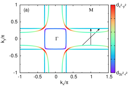
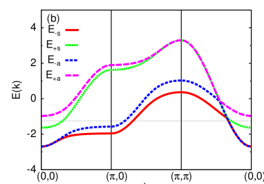
Figure 1: (a) Calculated Fermi surfaces for La_1.2Sr_1.8Mn₂O₇ with $d_{x^{2}-y^{2}}$ and $d_{3z^{2}-r^{2}}$ orbital densities, and (b) electronic dispersion in the high-symmetry directions for the crystal-field parameter $\Delta=-0.3$, the chemical potentials $\mu=-1.26$, and the inter-planar hopping $t_{\perp}=0.33$.

To reproduce the experimental Fermi surfaces with the above dispersion, we choose the values of chemical potential $\mu$ = -1.26, inter-planar hopping parameter $t_{\perp}=0.33$, and crystal-field parameter $\Delta=0.3$ in the unit of $t_{\parallel}=t$. The chemical potential $\mu$ = -1.26 corresponds to the $e_{g}$ electron density of $1-x\approx 0.54$/Mn, inter-planar hopping controls the splitting of the hole pockets around X, and crystal-field parameter improves the nesting quality by straightening the hole pockets as shown in Fig. 1(a). The electron pocket around the $\Gamma$ point and two hole pockets around the M point with one having almost straight segments belonging to the lower of plane-symmetric bands (bonding band) are in good agreement with the ARPES measurements.zsun4 The electron pocket has predominantly $d_{3z^{2}-r^{2}}$ orbital character whose proportion decreases only slightly on moving from $\Gamma$-M to $\Gamma$-X direction. Both the hole pockets have large $d_{x^{2}-y^{2}}$ orbital character in the $\Gamma$-M direction. In addition, the hole pocket belonging to the lower of plane-antisymmetric band (antibonding band) contains an almost equal mixture of $d_{x^{2}-y^{2}}$ and $d_{3z^{2}-r^{2}}$ orbitals near X at the zone boundary, whereas the hole pocket belonging to the bonding band consists mainly of $d_{3z^{2}-r^{2}}$ orbital. Similar features were also obtained in the band-structure calculations.saniz Particularly along the $\Gamma$-M direction, since the orbital mixing vanishes, the electronic states on the electron and hole Fermi surface have the orbital characters of $d_{3z^{2}-r^{2}}$ and $d_{x^{2}-y^{2}}$, respectively. There exist both intra-band (bonding-bonding or antibonding-antibonding) and inter-band (bonding-antibonding) nestings. From Fig. 1(a), the nesting vectors for the bonding-bonding, antibonding-antibonding, and bonding-antibonding nestings are expected at $\{(0.6\pi,0),(0.6\pi,0.6\pi)\}$, $\{(0.4\pi,0),(0.4\pi,0.4\pi)\}$, and $\{(0.5\pi,0),(0.5\pi,0.5\pi)\}$, respectively. The quality of nesting decreases from the bonding-bonding to the bonding-antibonding case, and is the poorest for antibonding-antibonding nesting.

III Orbital Fluctuation

To identify the important low energy orbital excitations in the ferromagnetic-metallic phase of the bilayer manganites with the spin degree of freedom already frozen, we investigate the orbital susceptibility of a bilayer lattice system with two orbitals at each site, which, in general, will be a 16$\times$16 matrix as 16 different orbital operators can be defined due to the four different electron field operators corresponding to the orbital and planar degrees of freedom in a unit cell. But the relevant orbital susceptibility, which involves only the $intralayer$ orbital operators, can be written in a 8$\times$8 matrix form. A further simplification can be achieved by changing to a basis in the planar space, which involves orbital operators symmetric and antisymmetric with respect to the mirror symmetry between the two planes in a unit cell. The relevant orbital susceptibility reduces to two 4$\times$4 matrices in this basis resulting from the fact that the correlation functions involving symmetric and antisymmetric orbital operators vanish identically by the symmetry of the bilayer Hamiltonian, and therefore can be defined as follows:

$$\chi^{m}_{ll^{\prime}}({\bf q},i\Omega_{n})=2\int^{\beta}_{0}{d\tau e^{i\Omega_{n}\tau}\langle T_{\tau}[{\cal T}^{m}_{{\bf q}l}(\tau){\cal T}^{m}_{-{\bf q}l^{\prime}}(0)]\rangle}.$$ (15)

Here, $\langle...\rangle$ denotes thermal average, $T_{\tau}$ imaginary time ordering, and $\Omega_{n}$ are the Bosonic Matsubara frequencies. ${\cal T}^{m}_{{\bf q}l}$ is the Fourier ${\bf q}$-component of orbital operator ${\cal T}^{m}_{{\bf i}l}$ symmetric ($m=s$) and antisymmetric ($m=a$) with respect to the mirror symmetry between the two planes in a unit cell. The symmetric and antisymmetric components are given by

$${\cal T}^{s}_{{\bf q}l}=({\cal T}^{1}_{{\bf q}l}+{\cal T}^{2}_{{\bf q}l})/2,\,\,\,\,\,{\cal T}^{a}_{{\bf q}l}=({\cal T}^{1}_{{\bf q}l}-{\cal T}^{2}_{{\bf q}l})/2,$$ (16)

respectively.

Expression for the relevant RPA-level orbital susceptibility is given bytakimoto

$$\hat{\chi}^{s(a)}({\bf q},i\Omega_{n})\!=\!\hat{\chi}^{0;s(a)}({\bf q},i\Omega_{n})[\hat{1}+\hat{U}\hat{\chi}^{0;s(a)}({\bf q},i\Omega_{n})]^{-1}.$$ (17)

After a unitary transformation, row and column labels appear in the order 11, 22, 12, and 21 with 1 and 2 as orbital indices. $\hat{1}$ is a 4$\times$4 matrix. The matrix elements of $\hat{\chi}^{0;s(a)}({\bf q},i\Omega_{n})$ are defined as

$$\chi^{0;s}_{\mu\nu,\alpha\beta}({\bf q},i\Omega_{n}) = (\chi^{0;aa,aa}_{\mu\nu,\alpha\beta}({\bf q},i\Omega_{n})+\chi^{0;ss,ss}_{\mu\nu,\alpha\beta}({\bf q},i\Omega_{n}))/2$$

$$\chi^{0;a}_{\mu\nu,\alpha\beta}({\bf q},i\Omega_{n}) = (\chi^{0;as,as}_{\mu\nu,\alpha\beta}({\bf q},i\Omega_{n})+\chi^{0;sa,sa}_{\mu\nu,\alpha\beta}({\bf q},i\Omega_{n}))/2,$$ (18)

where $\chi^{0;rs,uv}_{\mu\nu,\alpha\beta}({\bf q},i\Omega_{n})$= $-T\sum_{{\bf k},m}G^{ru}_{\alpha\mu}({\bf k}+{\bf q},i\omega_{m}+i\Omega_{n})G^{sv}_{\nu\beta}({\bf k},i\omega_{m})$, and $G^{sv}_{\nu\beta}({\bf k},i\omega_{n})$ is block diagonalized with respect to the superscripts ($s$ and $v$) as already discussed in the previous section. The bare symmetric and antisymmetric susceptibilities can be expressed explicitly as follows

$$\chi^{0;s}_{\mu\nu,\alpha\beta}({\bf q},i\Omega_{n})=-\frac{1}{N}\sum_{{\bf k}}\sum_{i,j}\sum_{\pm}\sum_{p=s,a}a^{\mu p^{*}}_{j{\bf k}+{\bf q}}a^{\nu p}_{i{\bf k}}a^{\beta p^{*}}_{i{\bf k}}a^{\alpha p}_{j{\bf k}+{\bf q}}\frac{n(E^{p}_{i}({\bf k}))-n(E^{p}_{j}({\bf k}+{\bf q}))}{i\Omega_{n}+E^{p}_{i}({\bf k})-E^{p}_{j}({\bf k}+{\bf q})}$$

$$\chi^{0;a}_{\mu\nu,\alpha\beta}({\bf q},i\Omega_{n})=-\frac{1}{N}\sum_{{\bf k}}\sum_{i,j}\sum_{\pm}\sum_{p=s,a}a^{\mu\bar{p}^{*}}_{j{\bf k}+{\bf q}}a^{\nu p}_{i{\bf k}}a^{\beta p^{*}}_{i{\bf k}}a^{\alpha\bar{p}}_{j{\bf k}+{\bf q}}\frac{n(E^{p}_{i}({\bf k}))-n(E^{\bar{p}}_{j}({\bf k}+{\bf q}))}{i\Omega_{n}+E^{p}_{i}({\bf k})-E^{\bar{p}}_{j}({\bf k}+{\bf q})},$$ (19)

where $a^{\nu p}_{i}$s are the unitary coefficients of the $i$-band to $\nu$-orbital obtained from Eq. (13), and $n(\xi)$ is the Fermi distribution function. Finally, the interaction matrix is given by

$$\hat{U}=\left\{\begin{array}[]{@{\,} l @{\,} c}-U&(\mu=\alpha\neq\nu=\beta)\\ U&(\mu=\nu\neq\alpha=\beta)\\ 0&(\mathrm{otherwise})\end{array}\right.,$$ (20)

where the parameter $U$ has been used for the inter-orbital Coulomb interaction from now on.

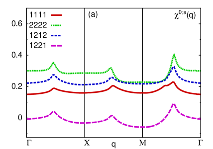
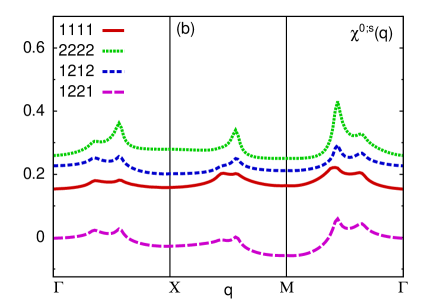
Figure 2: Principal components contributing to the transverse and longitudinal susceptibility for the (a) antisymmetric and (b) symmetric case. The antisymmetric and symmetric susceptibility show peaks at $\{(0.5\pi,0)$, $(0.5\pi,0.5\pi)\}$ and $\{(0.6\pi,0)$, $(0.6\pi,0.6\pi)\}$, respectively.

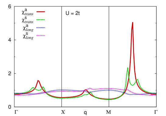
Figure 3: RPA level transverse and longitudinal susceptibilities for symmetric and antisymmetric case $U=2.0t$. Electronic correlation enhances the the antisymmetric transversal orbital susceptibility at $(0.5\pi,0.5\pi$) more in comparison to others.

Fig. 2 shows the principal components of one bubble static orbital susceptibility for the chemical potential $\mu$ = -1.26, interplane hopping parameter $t_{\perp}$ = 0.33, and temperature $T=0.02$. The components of antisymmetric susceptibility exhibit peak structures at $\{(0.5\pi,0)$, $(0.5\pi,0.5\pi)\}$ and those of symmetric show peaks at $\{(0.6\pi,0)$, $(0.6\pi,0.6\pi)\}$ as shown in Fig. 2(a) and 2(b), respectively. In the case of $\chi^{0;}_{1212}({\bf q})$ and $\chi^{0;}_{1221}({\bf q})$ contributing to the transverse orbital susceptibility, the antisymmetric components display a sharper and relatively larger peaks at $(0.5\pi,0.5\pi)$ in comparison to the symmetric components at $(0.6\pi,0.6\pi)$, and viceversa for the components $\chi^{0;}_{1111}({\bf q})$ and $\chi^{0;}_{2222}({\bf q})$ contributing to the charge or longitudinal orbital susceptibility. The above features are sensitive to both the orbital composition and the quality of nesting. For instance, $\chi^{0;s}_{2222}({\bf q})$ shows largest peaks at $(0.6\pi,0.6\pi)$ reflecting the straight segments of the Fermi surfaces dominated by $d_{3z^{2}-r^{2}}$ orbital. On the other hand, both $\chi^{0;a}_{1212}({\bf q})$ and $\chi^{0;a}_{1221}({\bf q})$ are enhanced at $(0.5\pi,0.5\pi)$ due to the nesting between the bonding Fermi surface consisting predominantly of $d_{3z^{2}-r^{2}}$ orbital and the antibonding Fermi surface having an almost equal mixture of both the orbitals although the nesting is relatively weaker than the bonding-bonding case. The longitudinal susceptibility is rendered featureless as the peak structure of $\chi^{0;s}_{2222}({\bf q})$ is subtracted out by the peak structure of $\chi^{0;s}_{1122}({\bf q})$ which is equal to the $\chi^{0;s}_{1221}({\bf q})$.

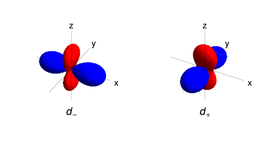
Figure 4: $d_{\mp}=\frac{1}{\sqrt{2}}(d_{3z^{2}-r^{2}}\,{\mp}\,d_{x^{2}-y^{2}}$) orbitals with red and blue colors highlighting the phases.

Fig. 3 shows the longitudinal $\chi_{zz}({\bf q})$ and the transverse $\chi_{xx}({\bf q})$ orbital susceptibilities calculated within the RPA. Transverse antisymmetric susceptibility is enhanced significantly at ($0.5\pi,0.5\pi$) as compared to the symmetric susceptibility at ($0.6\pi,0.6\pi$) due to the electronic interaction. On the other hand, the longitudinal susceptibilities are unaffected by the electronic interaction, and are almost featureless. Therefore, the bonding-antibonding band nesting is responsible for the strong and dominant orbital fluctuations at wavevector ($0.5\pi,0.5\pi$), with the nature of fluctuations being antisymmetric and transversal. In addition, we note that the transversal orbital susceptibility $\chi_{xx}({\bf q})$ is nothing but the longitudinal orbital susceptibility $\chi_{z^{\prime}z^{\prime}}({\bf q})$ in a new basis consisting of $d_{-}$ and $d_{+}$ orbitals, where $d_{\mp}=\frac{1}{\sqrt{2}}(d_{3z^{2}-r^{2}}\,{\mp}\,d_{x^{2}-y^{2}}$) (Fig. 4). Similarly, the longitudinal susceptibility $\chi_{zz}({\bf q})$ in the original basis is equal to the transverse susceptibility $\chi_{x^{\prime}x^{\prime}}({\bf q})$. Then, the fact that the longitudinal susceptibilities $\chi_{x^{\prime}x^{\prime}}({\bf q})$ (transverse susceptibilities in the new basis) are featureless and the transverse susceptibilities $\chi_{z^{\prime}z^{\prime}}({\bf q})$ (longitudinal susceptibilities in the basis) show peak structures follows from the orbital compositions of the Fermi surface, which consists predominantly of $d_{-}$ and $d_{+}$ orbitals along $k_{x}/\pi$ $\approx\pm$ 0.3 (or $\pm$0.2) and $k_{y}/\pi$ $\approx$ $\pm$0.3 (or $\pm$0.2), respectively as shown in Fig. 5.

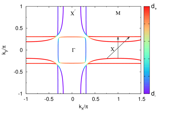
Figure 5: Orbital densities of $d_{-}$ and $d_{+}$ orbitals on the Fermi surface for the crystal-field parameter $\Delta=-0.3$, the chemical potentials $\mu=-1.26$, and the inter-planar hopping $t_{\perp}=0.33$.

IV Phonon renormalization

Since strong antisymmetric orbital fluctuations are present due to the correlations, which couples to the antisymmetric component of transversal Jahn-Teller phonons, we consider the impact of these orbital fluctuations on the phonon propagator in this section. The second-order perturbation theory with respect to the last term of the Hamiltonian given by Eq. (1) provides the following self-energy of transversal Jahn-Teller phononsallen ; maier

$$\Sigma^{s(a)}({\bf q},\Omega+i\delta)=-g^{2}\sum_{\mu\nu}\chi^{s(a)}_{\mu\bar{\mu},\nu\bar{\nu}}({\bf q},\Omega+i\delta),$$ (21)

where

$$\chi^{s(a)}_{\mu\bar{\mu},\nu\bar{\nu}}({\bf q},\Omega+i\delta)=[\hat{\chi}^{0;s(a)}({\bf q},\Omega+i\delta)[\hat{1}+\hat{U}\hat{\chi}^{0;s(a)}({\bf q},\Omega+i\delta)]^{-1}]_{\mu\bar{\mu},\nu\bar{\nu}}.$$ (22)

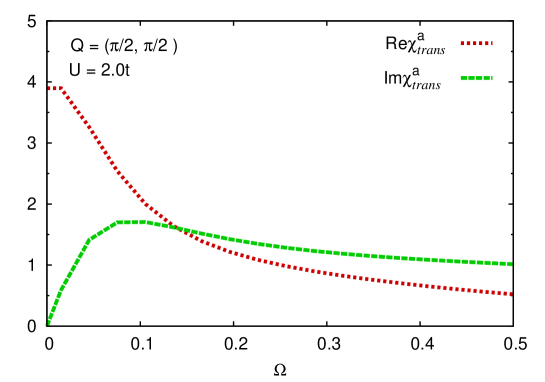
Figure 6: Real and imaginary parts of the antisymmetric transverse orbital susceptibility as a function frequency at fixed momentum ${\bf q}=(0.5\pi,0.5\pi)$.

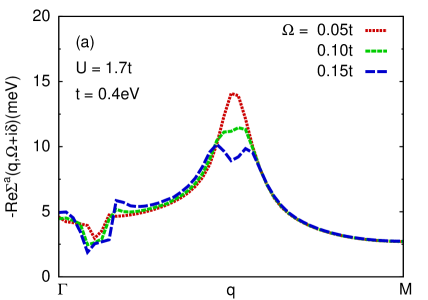
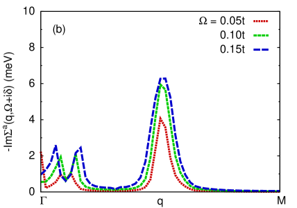
Figure 7: (a) Real and (b) imaginary part of the antisymmetric phonon self-energy arising due to the antisymmetric transversal orbital fluctuation mode at wavevector (0.5$\pi$, 0.5$\pi$).

Fig. 6 shows the real and imaginary part of $\chi^{a}_{trans}({\bf q},\Omega+i\delta)$ for (0.5$\pi$, 0.5$\pi$) as a function of frequency, where the imaginary part shows a maximum near $\Omega\approx 0.1t$ which provides the order of energy scale of the fluctuation. Fig. 7 shows the real and imaginary part of the phonon self-energy for several values of frequency $\Omega$ around the energy scale of antisymmetric transverse orbital fluctuation. Here, the frequencies are chosen of the same order as that of local Jahn-Teller distortion frequency $\Omega^{*}\approx 50meV$ determined from Raman scatterings,allen ; iliev which can be estimated roughly to be $\Omega^{*}\approx 0.1t$ with $t$ $\approx 0.4eV$.dagotto We have chosen the electron-phonon coupling parameter $g\approx 0.125t$ to reproduce the experimental result as shown in Fig. 7. There is a large self-energy correction to antisymmetric component of transversal Jahn-Teller phonons near (0.5$\pi$, 0.5$\pi$, 0) where the linewidth also exhibits maximum. Both these features show a good quantitative agreement with the neutron scattering experiments for phonons in the ferromagnetic-metallic bilayers.weber

We also find additional peaks in the the linewidth and dip in the self-energy for the low-momentum region. Already existing on either side of $|{\bf q}|\approx 0.1\pi$ at the bare level, these peaks appear due to the saddle point behavior of $E^{a}_{-}({\bf k+q})-E^{s}_{-}({\bf k})$ and $E^{s}_{-}({\bf k+q})-E^{a}_{-}({\bf k})$ in the denominator of the antisymmetric susceptibility for $|{\bf q}|\geq 0.1\pi$ or $|{\bf q}|\leq 0.1\pi$, respectively. Saddle points lie near ${\bf k}$ = ($-0.3\pi,\mp\pi$) and ($\mp\pi,-0.3\pi$) with maximum along $k_{x}$ and minimum along $k_{y}$ for $E^{a}_{-}({\bf k+q})-E^{s}_{-}({\bf k})$, and near ${\bf k}$ = $(0.3\pi,\mp\pi)$ and $(\mp\pi,0.3\pi)$ with minimum along $k_{x}$ and maximum along $k_{y}$ for $E^{s}_{-}({\bf k+q})-E^{a}_{-}({\bf k})$. The movement in the opposite directions and enhancement of the peaks away from $|{\bf q}|\approx 0.1\pi$ with increasing energy follows from the movement towards the saddle point which lies only slightly away from the Fermi surface in each case. The origin of these peak structures, therefore, is analogous to that of peak found in the density of states near the saddle point of the energy band in the momentum space. Thus, our study suggests additional peaks to be observed in the inelastic neutron scattering experiments in low-momentum region.

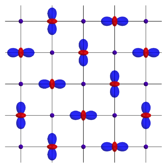
Figure 8: Orbital correlations with wavevector (0.5$\pi$, 0.5$\pi$) developed in the ferromagnetic metallic La_1.2Sr_1.8Mn₂O₇ involving $d_{\mp}$ orbitals, where electrons hop along zigzag chains in $x$ and $y$ directions through $d_{-}$ and $d_{+}$ orbitals, an essential mechanism to stabilize the CE-type spin arrangement.

V Conclusions and Discussions

Our investigation of the orbital fluctuations in a bilayer system with two orbitals at each site, which captures the salient features of the ARPES measurements for the ferromagnetic-metallic phase of the doped bilayer manganite La_1.2Sr_1.8Mn₂O₇ has provided an important connection between the the Fermi-surface structure and the short-range dynamical correlations as observed in the neutron scattering experiments. Antisymmetric longitudinal orbital fluctuations in the basis of $d_{-}$ and $d_{+}$ orbitals are strong at ($0.5\pi,0.5\pi$), where $d_{\mp}=\frac{1}{\sqrt{2}}(d_{3z^{2}-r^{2}}\,{\mp}\,d_{x^{2}-y^{2}})$. This follows from the Fermi-surface nesting between bonding and antibonding bands instead of the nesting between bonding and bonding bands despite their flat segments. Moreover, the orbital fluctuations strongly renormalize the antisymmetric component of transversal Jahn-Teller phonons near wavevector (0.5$\pi$, 0.5$\pi$), and are responsible for the shortest lifetime of the phonons near the same wavevector, implying their dynamic nature. Our study also predicts the enhancement of phonon linewidth near the low momentum region, which should be observed in the inelastic neutron scattering experiments.

The proximity to the orbital ordering instability of La_1.2Sr_1.8Mn₂O₇ due to the strong nesting with orbital compositions of the Fermi surface predominantly of $d_{-}$ and $d_{+}$ orbitals along $k_{x}/\pi$ $\approx\pm$ 0.3 (or $\pm$0.2) and $k_{y}/\pi$ $\approx$ $\pm$0.3 (or $\pm$0.2) is suppressed by the ferromagnetism stabilized by the double-exchange mechanism.zener In such orbitally correlated or ordered state, the electrons will prefer to hop along $x$ and $y$ directions through $d_{-}$ and $d_{+}$ orbitals as shown in Fig. 8, which may instead support a CE-type spin arrangement wherein spins are aligned ferromagnetically along the zigzag chains. Therefore, our study provides a plausible explanation for the existence of CE-type orbital fluctuations in the ferromagnetic-metallic bilayer near $x=0.4$ as observed in the neutron scattering experiments.

References

- (1) R. von Helmolt, J. Wecker, B. Holzapfe, L. Schultz, and K. Samwer, Phys. Rev. Lett. 71, 2331 (1993).
- (2) S. Jin, T. H. Tiefel, M. McCormack, R. A. Fastnacht, R. Ramesh, and L. H. Chen, Science 264, 413 (2004).
- (3) C. Şen, G. Alvarez, and E. Dagotto, Phys. Rev. Lett. 105, 097203 (2010).
- (4) F. Weber, N. Aliouane, H. Zheng, J. F. Mitchell, D. N. Argyriou, and D. Reznik, Nature Mater. 8, 798 (2009).
- (5) E Saitoh, Y Tomioka, T Kimura, and Y Tokura, J. Magn. Magn. Mater. 239, 170 (2002).
- (6) C. P. Adams, J.W. Lynn, Y. M. Mukovskii, A. A. Arsenov, and D. A. Shulyatev, Phys. Rev. Lett. 85, 3954 (2000).
- (7) F. Moussa, M. Hennion, P. Kober-Lehouelleur, D. Reznik, S. Petit, H. Moudden, A. Ivanov, Ya. M. Mukovskii, R. Privezentsev, and F. Albenque-Rullier, Phys. Rev. B 76, 064403 (2007).
- (8) E. O. Wollan and W. C. Koehler, Phys. Rev. 100, 545 (1955).
- (9) J. B. Goodenough, Phys. Rev. 100, 564 (1955).
- (10) H. Y. Hwang, P. Dai, S-W. Cheong, G. Aeppli, D. A. Tennant, and H. A. Mook, Phys. Rev. Lett. 80, 1316 (1998).
- (11) F. Ye, P. Dai, J. A. Fernandez-Baca, H. Sha, J.W. Lynn, H. Kawano- Furukawa, Y. Tomioka, Y. Tokura, and J. Zhang, Phys. Rev. Lett. 96, 047204 (2006).
- (12) D. K. Singh, B. Kamble, and A. Singh, Phys. Rev. B 81, 064430 (2010).
- (13) D. K. Singh, B. Kamble, and A. Singh, J. Phys.: Condens. Matter 22, 396001 (2010).
- (14) Y. Moritomo, A. Asamitsu, H. Kuwahara, and Y. Tokura, Nature 380, 141 (1996).
- (15) J. F. Mitchell, D. N. Argyriou, J. D. Jorgensen, D. G. Hinks, C. D. Potter, and S. D. Bader, Phys. Rev. B 55, 63-6 (1997).
- (16) Y.-D. Chuang, A. D. Gromko, D. S. Dessau, T. Kimura, and Y. Tokura, Science 292, 1509 (2001).
- (17) N. Mannella, W. L. Yang, X. J. Zhou, H. Zheng, J. F. Mitchell, J. Zaanen, T. P. Devereaux, N. Nagaosa, Z. Hussain, and Z.-X. Shen, Nature 438, 474 (2005).
- (18) D.V. Evtushinsky, D. S. Inosov, G. Urbanik, V. B. Zabolotnyy, R. Schuster, P. Sass, T. Hänke, C. Hess, B. Büchner, R. Follath, P. Reutler, A. Revcolevschi, A. A. Kordyuk, and S.V. Borisenko, Phys. Rev. Lett. 105, 147201 (2010).
- (19) Z. Sun, Y.-D. Chuang, A.V. Fedorov, J. F. Douglas, D. Reznik, F.Weber, N. Aliouane, D. N. Argyriou, H. Zheng, J. F. Mitchell, T. Kimura, Y. Tokura, A. Revcolevschi, and D. S. Dessau, Phys. Rev. Lett. 97, 056401 (2006).
- (20) S. de Jong, F. Massee, Y. Huang, M. Gorgoi, F. Schaefers, J. Fink, A. T. Boothroyd, D. Prabhakaran, J. B. Goedkoop, and M. S. Golden, Phys. Rev. B 80, 205108 (2009).
- (21) Z. Sun, J. F. Douglas, A. V. Fedorov, Y.-D. Chuang, H. Zheng, J. F. Mitchell, and D. S. Dessau, Nature Phys. 3, 248 (2007).
- (22) F. Massee, S. de Jong, Y. Huang, W. K. Siu, I. Santoso, A. Mans, A. T. Boothroyd, D. Prabhakaran, R. Follath, A. Varykhalov, L. Patthey, M. Shi, J. B. Goedkoop, and M. S. Golden, Nature Phys. 7, 978 (2011).
- (23) Z. Sun, Q. Wang, J. F. Douglas, Y.-D. Chuang, A. V. Fedorov, E. Rotenberg, H. Lin, S. Sahrakorpi, B. Barbiellini, R. S. Markiewicz, A. Bansil, H. Zheng, J. F. Mitchell, and D. S. Dessau, Phys. Rev. B 86, 201103 (2012).
- (24) Z. Sun, Y.-D. Chuang, A.V. Fedorov, J. F. Douglas, D. Reznik, F.Weber, N. Aliouane, D. N. Argyriou, H. Zheng, J. F. Mitchell, T. Kimura, Y. Tokura, A. Revcolevschi, and D. S. Dessau, Phys. Rev. Lett. 97, 056401 (2006).
- (25) E. Dagotto, T. Hotta, and A. Moreo, Phys. Rep. 344 1 (2001).
- (26) I. Eremin, D. K. Morr, A. V. Chubukov, and K. Bennemann, Phys. Rev. B 75, 184534 (2007).
- (27) R. Saniz, M. R. Norman, and A. J. Freeman, Phys. Rev. Lett. 101, 236402 (2008).
- (28) T. Takimoto, T. Hotta, T. Maehira, and K. Ueda, J. Phys.: Condens. Matter 14, L369-L375 (2002).
- (29) P. B. Allen, Phys. Rev. B 6, 2577 (1972).
- (30) T. A. Maier, S. Graser, P. J. Hirschfeld, and D. J. Scalapino, Phys. Rev. B 83, 220505 (2011).
- (31) V. Perebeinos and P. B. Allen, Phys. Rev. Lett. 85, 5178 (2000).
- (32) M. N. Iliev, M. V. Abrashev, H.-G. Lee, V. N. Popov, Y. Y. Sun, C. Thomsen, R. L. Meng, and C. W. Chu, Phys. Rev. B 57, 2872 (1998).
- (33) C. Zener, Phys. Rev. 82, 403 (1951).