Optimal Starting-Stopping and Switching of a CIR Process
with Fixed Costs

Abstract

This paper analyzes the problem of starting and stopping a Cox-Ingersoll-Ross (CIR) process with fixed costs. In addition, we also study a related optimal switching problem that involves an infinite sequence of starts and stops. We establish the conditions under which the starting-stopping and switching problems admit the same optimal starting and/or stopping strategies. We rigorously prove that the optimal starting and stopping strategies are of threshold type, and give the analytical expressions for the value functions in terms of confluent hypergeometric functions. Numerical examples are provided to illustrate the dependence of timing strategies on model parameters and transaction costs.

Keywords:  optimal starting-stopping, optimal switching, CIR process, confluent hypergeometric functions
JEL Classification:  C41, G11, G12
Mathematics Subject Classification (2010):  60G40, 91G10, 62L15

1 Introduction

Many problems in risk analysis and finance involve a sequence of starting and stopping decisions. For instance, a trader may seek the optimal times to buy and then sell an asset, or a firm may seek to invest in a project and subsequently sell it to another firm. This motivates us to study an optimal starting-stopping (or entry-exit) timing problem.

In general, the optimal timing depends crucially on the dynamics of the underlying process. In particular, if the process is a super/sub-martingale, such as the geometric Brownian motion, then it is optimal either to stop immediately or wait forever (see e.g. Shiryaev et al. (2008)). As such, the corresponding optimal single stopping, starting-stopping, or switching problems will admit a trivial solution. In this paper, our optimal starting-stopping and switching problems are driven by the Cox-Ingersoll-Ross (CIR) process (see Cox et al. (1985)). The CIR process has been widely used as the model for interest rates, volatility, and energy prices (see, for example, Cox et al. (1985), Heston (1993), Ribeiro and Hodges (2004), respectively). In the real option literature, mean reverting processes have been used to model the value of a project. For instance, Ewald and Wang (2010) studies the timing of an irreversible investment whose value is modeled by a CIR process, and they solve the associated optimal single stopping problem. Carmona and León (2007) examine the optimal investment timing where the interest rate evolves according to a CIR process. Other mean-reverting models, such as the exponential Ornstein-Uhlenbeck (OU) model, have been discussed in Dixit (1994). In contrast to these studies, our model addresses multiple timing decisions.

Our main contribution is the analytical derivation of the non-trivial optimal starting and stopping timing strategies and the associated value functions. Under both starting-stopping and switching approaches, it is optimal to stop when the process value is sufficiently high, though at different levels. As for starting timing, we find the necessary and sufficient conditions whereby it is optimal not to start at all when facing the optimal switching problem. In this case, the optimal switching problem in fact reduces into an optimal single stopping problem, where the optimal stopping level is identical to that of the optimal starting-stopping problem.

In the literature, Menaldi et al. (1996) study an optimal starting-stopping problem for general Markov processes, and provide the mathematical characterization of the value functions. Sun (1992) considers an optimal starting-stopping problem driven by a time-homogeneous diffusion, and analyzes the associated nested variational inequalities (VIs). Zervos et al. (2013) discusses a solution methodology involving coupled variational inequalities for an optimal switching problem under some time-homogeneous diffusions subject to fixed transaction costs. Tanaka (1993) studies an optimal starting-stopping problem for two-parameter stochastic processes under discrete time.

The VI approach is commonly used not only for optimal starting-stopping and switching problems, but also for optimal stopping problems (see Bensoussan and Lions (1982) and Øksendal (2003), among others). The VI method is most useful when the reward and value functions are simple explicit functions with amenable properties. In our starting-stopping problem, however, the reward function for the starting problem is expressed in terms of the confluent hypergeometric function of the first kind and can be positive or negative. This motivates us to adopt a probabilistic approach to rigorously construct the value functions. In contrast to the VI approach, we solve the optimal starting-stopping problem by characterizing the value functions as the decreasing smallest concave majorant of the corresponding reward functions. This allows us to directly derive the value function and prove its optimality, without a priori conjecturing the resulting regions for starting/stopping/continuation. This methodology has been discussed in Dayanik and Karatzas (2003), dating back to Dynkin and Yushkevich (1969). Having solved the optimal starting-stopping problem, we then apply our results to infer a similar solution structure for the optimal switching problem and verify using the variational inequalities.

As for related applications of optimal starting-stopping problems, Leung and Li (2014) study the optimal timing to trade a mean-reverting price spread with a stop-loss constraint. Leung et al. (2014) investigate the problem of buying and selling an exponential-OU underlying subject to transaction costs. Karpowicz and Szajowski (2007) analyze the starting-stopping times for a risk process for an insurance firm. In the context of derivatives trading, Leung and Liu (2012) study the optimal timing to liquidate credit derivatives where the default intensity is modeled by an OU or CIR process. They focus on the finite-horizon trading problem, and identify the conditions under which immediate stopping or perpetual holding is optimal.

The rest of the paper is structured as follows. In Section 2, we formulate both the optimal starting-stopping and optimal switching problems. Then, we present our analytical results and numerical examples in Section 3. The proofs of our main results are detailed in Section 4. Finally, the Appendix contains the proofs for a number of lemmas.

2 Problem Overview

Denote the probability space by $(\Omega,{\mathcal{F}},{\mathbb{P}})$, where ${\mathbb{P}}$ is the historical probability measure. We consider a CIR process $(Y_{t})_{t\geq 0}$ that satisfies the SDE

$$dY_{t}=\mu(\theta-Y_{t})\,dt+\sigma\sqrt{Y_{t}}\,dB_{t},$$ (2.1)

with constants $\mu,\theta,\sigma>0,$ and $B$ is a standard Brownian motion defined on the probability space. If $2\mu\theta\geq\sigma^{2}$ holds, which is often referred to as the Feller condition (see Feller (1951)), then the level $0$ is inaccessible by $Y$. If the initial value $Y_{0}>0$, then $Y$ stays strictly positive at all times almost surely. Nevertheless, if $Y_{0}=0$, then $Y$ will enter the interior of the state space immediately and stays positive thereafter almost surely. If $2\mu\theta<\sigma^{2}$, then the level $0$ is a reflecting boundary. This means that once $Y$ reaches $0$, it immediately returns to the interior of the state space and continues to evolve. For a detailed categorization of boundaries for diffusion processes, we refer to Chapter 2 of Borodin and Salminen (2002) and Chapter 15 of Karlin and Taylor (1981).

2.1 Optimal Starting-Stopping Problem

Given a CIR process, we first consider the optimal timing to stop. If a decision to stop is made at some time $\tau$, then the amount $Y_{\tau}$ is received and simultaneously the constant transaction cost $c_{s}>0$ has to be paid. Denote by $\mathbb{F}$ the filtration generated by $B$, and ${\mathcal{T}}$ the set of all $\mathbb{F}$-stopping times. The maximum expected discounted value is obtained by solving the optimal stopping problem

$$V(y) =\sup_{\tau\in{\mathcal{T}}}\mathbb{E}_{y}\!\left\{e^{-r\tau}(Y_{\tau}-c_{s})\right\},$$ (2.2)

where $r>0$ is the constant discount rate, and $\mathbb{E}_{y}\{\cdot\}\equiv\mathbb{E}\{\cdot|Y_{0}=y\}$.

The value function $V$ represents the expected value from optimally stopping the process $Y$. On the other hand, the process value plus the transaction cost constitute the total cost to start. Before even starting, one needs to choose the optimal timing to start, or not to start at all. This leads us to analyze the starting timing inherent in the starting-stopping problem. Precisely, we solve

$$J(y) =\sup_{\nu\in{\mathcal{T}}}\mathbb{E}_{y}\!\left\{e^{-r\nu}(V(Y_{\nu})-Y_{\nu}-c_{b})\right\},$$ (2.3)

with the constant transaction cost $c_{b}>0$ incurred at the start. In other words, the objective is to maximize the expected difference between the value function $V(Y_{\nu})$ and the current $Y_{\nu}$, minus transaction cost $c_{b}$. The value function $J(y)$ represents the maximum expected value that can be gained by entering and subsequently exiting, with transaction costs $c_{b}$ and $c_{s}$ incurred, respectively, on entry and exit. For our analysis, the transaction costs $c_{b}$ and $c_{s}$ can be different. To facilitate presentation, we denote the functions

$$h_{s}(y)=y-c_{s},\quad\text{ and }\quad h_{b}(y)=y+c_{b}.$$ (2.4)

If it turns out that $J(Y_{0})\leq 0$ for some initial value $Y_{0}$, then it is optimal not to start at all. Therefore, it is important to identify the trivial cases. Under the CIR model, since $\sup_{y\in{\mathbb{R}}_{+}}(V(y)-h_{b}(y))\leq 0$ implies that $J(y)=0$ for $y\in{\mathbb{R}}_{+}$, we shall therefore focus on the case with

$$\sup_{y\in{\mathbb{R}}_{+}}(V(y)-h_{b}(y))>0,$$ (2.5)

and solve for the non-trivial optimal timing strategy.

2.2 Optimal Switching Problem

Under the optimal switching approach, it is assumed that an infinite number of entry and exit actions take place. The sequential entry and exit times are modeled by the stopping times $\nu_{1},\tau_{1},\nu_{2},\tau_{2},\dots\in{\mathcal{T}}$ such that

$$0\leq\nu_{1}\leq\tau_{1}\leq\nu_{2}\leq\tau_{2}\leq\dots.$$

Entry and exit decisions are made, respectively, at times $\nu_{i}$ and $\tau_{i}$, $i\in\mathbb{N}$. The optimal timing to enter or exit would depend on the initial position. Precisely, under the CIR model, if the initial position is zero, then the first task is to determine when to start and the corresponding optimal switching problem is

$${\tilde{J}}(y) =\sup_{\Lambda_{0}}\mathbb{E}_{y}\left\{\sum_{n=1}^{\infty}[e^{-r\tau_{n}}h_{s}(Y_{\tau_{n}})-e^{-r\nu_{n}}h_{b}(Y_{\nu_{n}})]\right\},$$ (2.6)

with the set of admissible stopping times $\Lambda_{0}=(\nu_{1},\tau_{1},\nu_{2},\tau_{2},\dots)$, and the reward functions $h_{b}$ and $h_{s}$ defined in (2.4). On the other hand, if we start with a long position, then it is necessary to solve

$${\tilde{V}}(y) =\sup_{\Lambda_{1}}\mathbb{E}_{y}\left\{e^{-r\tau_{1}}h_{s}(Y_{\tau_{1}})+\sum_{n=2}^{\infty}[e^{-r\tau_{n}}h_{s}(Y_{\tau_{n}})-e^{-r\nu_{n}}h_{b}(Y_{\nu_{n}})]\right\},$$ (2.7)

with $\Lambda_{1}=(\tau_{1},\nu_{2},\tau_{2},\nu_{3},\dots)$ to determine when to stop.

In summary, the optimal starting-stopping and switching problems differ in the number of entry and exit decisions. Observe that any strategy for the starting-stopping problem (2.2)-(2.3) is also a candidate strategy for the switching problem (2.6)-(2.7). Therefore, it follows that $V(y)\leq{\tilde{V}}(y)$ and $J(y)\leq{\tilde{J}}(y).$ Our objective is to derive and compare the corresponding optimal timing strategies under these two approaches.

3 Summary of Analytical Results

We first summarize our analytical results and illustrate the optimal starting and stopping strategies. The method of solutions and their proofs will be discussed in Section 4. We consider the optimal starting-stopping problem followed by the optimal switching problem. First, we denote the infinitesimal generator of $Y$ as

$${\mathcal{L}} =\frac{\sigma^{2}y}{2}\frac{d^{2}}{dy^{2}}+\mu(\theta-y)\frac{d}{dy},$$ (3.1)

and consider the ordinary differential equation (ODE)

$${\mathcal{L}}u(y)=ru(y),\quad\textrm{ for }\,y\in{\mathbb{R}}_{+}.$$ (3.2)

To present the solutions of this ODE, we define the functions

$$F(y):=M(\frac{r}{\mu},\frac{2\mu\theta}{\sigma^{2}};\frac{2\mu y}{\sigma^{2}}),\quad\text{and}\quad G(y):=U(\frac{r}{\mu},\frac{2\mu\theta}{\sigma^{2}};\frac{2\mu y}{\sigma^{2}}),$$ (3.3)

where

$$M(a,b;z) =\sum_{n=0}^{\infty}\frac{a_{n}z^{n}}{b_{n}n!},\qquad a_{0}=1,~{}a_{n}=a(a+1)(a+2)\cdots(a+n-1),$$

$$U(a,b;z) =\frac{\Gamma(1-b)}{\Gamma(a-b+1)}M(a,b;z)+\frac{\Gamma(b-1)}{\Gamma(a)}z^{1-b}M(a-b+1,2-b;z)$$

are the confluent hypergeometric functions of first and second kind, also called the Kummer’s function and Tricomi’s function, respectively (see Chapter 13 of Abramowitz and Stegun (1965) and Chapter 9 of Lebedev (1972)). As is well known (see Göing-Jaeschke and Yor (2003)), $F$ and $G$ are strictly positive and, respectively, the strictly increasing and decreasing continuously differentiable solutions of the ODE (3.2). Also, we remark that the discounted processes $(e^{-rt}F(Y_{t}))_{t\geq 0}$ and $(e^{-rt}G(Y_{t}))_{t\geq 0}$ are martingales.

In addition, recall the reward functions defined in (2.4) and note that

$$({\mathcal{L}}-r)h_{b}(y)\begin{cases}>0&\,\textrm{ if }\,y<y_{b},\\ <0&\,\textrm{ if }\,y>y_{b},\end{cases}\quad\textrm{and}\quad({\mathcal{L}}-r)h_{s}(y)\begin{cases}>0&\,\textrm{ if }\,y<y_{s},\\ <0&\,\textrm{ if }\,y>y_{s},\end{cases}$$ (3.4)

where the critical constants $y_{b}$ and $y_{s}$ are defined by

$$y_{b}:=\frac{\mu\theta-rc_{b}}{\mu+r}\quad\textrm{and}\quad y_{s}:=\frac{\mu\theta+rc_{s}}{\mu+r}.$$ (3.5)

Note that $y_{b}$ and $y_{s}$ depend on the parameters $\mu,$ $\theta$ and $r$, as well as $c_{b}$ and $c_{s}$ respectively, but not $\sigma.$

3.1 Optimal Starting-Stopping Problem

We now present the results for the optimal starting-stopping problem (2.2)-(2.3). As it turns out, the value function $V$ is expressed in terms of $F$, and $J$ in terms of $V$ and $G$. The functions $F$ and $G$ also play a role in determining the optimal starting and stopping thresholds.

Theorem 3.1

The value function for the optimal stopping problem (2.2) is given by

$$V(y)=\begin{cases}\frac{b^{*}-c_{s}}{F(b^{*})}F(y)&\,\textrm{ if }\,y\in[0,b^{*}),\\ y-c_{s}&\,\textrm{ if }\,y\in[b^{*},+\infty).\end{cases}$$ (3.6)

Here, the optimal stopping level $b^{*}\in(c_{s}\vee y_{s},\infty)$ is found from the equation

$$F(b)=(b-c_{s}){F}^{\prime}\!(b).$$ (3.7)

Therefore, it is optimal to stop as soon as the process $Y$ reaches $b^{*}$ from below. The stopping level $b^{*}$ must also be higher than the fixed cost $c_{s}$ as well as the critical level $y_{s}$ defined in (3.5).

Now we turn to the optimal starting problem. Define the reward function

$$\hat{h}(y):=V(y)-(y+c_{b}).$$ (3.8)

Since $F$, and thus $V$, are convex, so is $\hat{h}$, we also observe that the reward function $\hat{h}(y)$ is decreasing in $y$. To exclude the scenario where it is optimal never to start, the condition stated in (2.5), namely, $\sup_{y\in{\mathbb{R}}+}\hat{h}(y)>0$, is now equivalent to

$$V(0)=\frac{b^{*}-c_{s}}{F(b^{*})}>c_{b},$$ (3.9)

since $F(0)=1$.

Theorem 3.2

The optimal starting problem (2.3) admits the solution

$$J(y)=\begin{cases}V(y)-(y+c_{b})&\,\textrm{ if }\,y\in[0,d^{*}],\\ \frac{V(d^{*})-(d^{*}+c_{b})}{G(d^{*})}G(y)&\,\textrm{ if }\,y\in(d^{*},+\infty).\end{cases}$$ (3.10)

The optimal starting level $d^{*}>0$ is uniquely determined from

$$G(d)({V}^{\prime}\!(d)-1)=G^{{}^{\prime}}\!(d)(V(d)-(d+c_{b})).$$ (3.11)

As a result, it is optimal to start as soon as the CIR process $Y$ falls below the strictly positive level $d^{*}$.

3.2 Optimal Switching Problem

Now we study the optimal switching problem under the CIR model in (2.1). We start by giving conditions under which it is optimal not to start ever.

Theorem 3.3

Under the CIR model, if it holds that

1. $y_{b}\leq 0,\quad\textrm{ or }$

2. $y_{b}>0\quad\textrm{ and }\quad c_{b}\geq\frac{b^{*}-c_{s}}{F(b^{*})},$

with $b^{*}$ given in (3.7), then the optimal switching problem (2.6)-(2.7) admits the solution

$$\tilde{J}(y)=0\qquad\textrm{for}\quad y\geq 0,$$ (3.12)

and

$$\tilde{V}(y)=\begin{cases}\frac{b^{*}-c_{s}}{F(b^{*})}F(y)&\,\textrm{ if }\,y\in[0,b^{*}),\\ y-c_{s}&\,\textrm{ if }\,y\in[b^{*},+\infty).\end{cases}$$ (3.13)

Conditions $(i)$ and $(ii)$ depend on problem data and can be easily verified. In particular, recall that $y_{b}$ is defined in (3.5) and is easy to compute, furthermore it is independent of $\sigma$ and $c_{s}$. Since it is optimal to never enter, the switching problem is equivalent to a stopping problem and the solution in Theorem 3.3 agrees with that in Theorem 3.1. Next, we provide conditions under which it is optimal to enter as soon as the CIR process reaches some lower level.

Theorem 3.4

Under the CIR model, if

$$y_{b}>0\quad\textrm{and}\quad c_{b}<\frac{b^{*}-c_{s}}{F(b^{*})},$$ (3.14)

with $b^{*}$ given in (3.7), then the optimal switching problem (2.6)-(2.7) admits the solution

$$\tilde{J}(y)=\begin{cases}KF(y)-(y+c_{b})&\,\textrm{ if }\,y\in[0,\tilde{d}^{*}],\\ QG(y)&\,\textrm{ if }\,y\in(\tilde{d}^{*},+\infty),\end{cases}$$ (3.15)

and

$$\tilde{V}(y)=\begin{cases}KF(y)&\,\textrm{ if }\,y\in[0,\tilde{b}^{*}),\\ QG(y)+(y-c_{s})&\,\textrm{ if }\,y\in[\tilde{b}^{*},+\infty),\end{cases}$$ (3.16)

where

$$K=\frac{G(\tilde{d}^{*})-(\tilde{d}^{*}+c_{b}){G}^{\prime}\!(\tilde{d}^{*})}{{F}^{\prime}\!(\tilde{d}^{*})G(\tilde{d}^{*})-F(\tilde{d}^{*}){G}^{\prime}\!(\tilde{d}^{*})},$$ (3.17)

$$Q=\frac{F(\tilde{d}^{*})-(\tilde{d}^{*}+c_{b}){F}^{\prime}\!(\tilde{d}^{*})}{{F}^{\prime}\!(\tilde{d}^{*})G(\tilde{d}^{*})-F(\tilde{d}^{*}){G}^{\prime}\!(\tilde{d}^{*})}.$$ (3.18)

There exist unique optimal starting and stopping levels $\tilde{d}^{*}$ and $\tilde{b}^{*}$, which are found from the nonlinear system of equations:

$$\frac{G(d)-(d+c_{b}){G}^{\prime}\!(d)}{{F}^{\prime}\!(d)G(d)-F(d){G}^{\prime}\!(d)} =\frac{G(b)-(b-c_{s}){G}^{\prime}\!(b)}{{F}^{\prime}\!(b)G(b)-F(b){G}^{\prime}\!(b)},$$ (3.19)

$$\frac{F(d)-(d+c_{b}){F}^{\prime}\!(d)}{{F}^{\prime}\!(d)G(d)-F(d){G}^{\prime}\!(d)} =\frac{F(b)-(b-c_{s}){F}^{\prime}\!(b)}{{F}^{\prime}\!(b)G(b)-F(b){G}^{\prime}\!(b)}.$$ (3.20)

Moreover, we have that $\tilde{d}^{*}<y_{b}\,\textrm{ and }\,\tilde{b}^{*}>y_{s}.$

In this case, it is optimal to start and stop an infinite number of times where we start as soon as the CIR process drops to $\tilde{d}^{*}$ and stop when the process reaches $\tilde{b}^{*}.$ Note that in the case of Theorem 3.3 where it is never optimal to start, the optimal stopping level $b^{*}$ is the same as that of the optimal stopping problem in Theorem 3.1. The optimal starting level $\tilde{d^{*}}$, which only arises when it is optimal to start and stop sequentially, is in general not the same as $d^{*}$ in Theorem 3.2.

We conclude the section with two remarks.

Remark 3.5

Given the model parameters, in order to identify which of Theorem 3.3 or Theorem 3.4 applies, we begin by checking whether $y_{b}\leq 0$. If so, it is optimal not to enter. Otherwise, Theorem 3.3 still applies if $c_{b}\geq\frac{b^{*}-c_{s}}{F(b^{*})}$ holds. In the other remaining case, the problem is solved as in Theorem 3.4. In fact, the condition $c_{b}<\frac{b^{*}-c_{s}}{F(b^{*})}$ implies $y_{b}>0$ (see the proof of Lemma 4.3 in the Appendix). Therefore, condition (3.14) in Theorem 3.4 is in fact identical to (3.9) in Theorem 3.2.

Remark 3.6

To verify the optimality of the results in Theorems 3.3 and 3.4, one can show by direct substitution that the solutions $(\tilde{J},\tilde{V})$ in (3.12)-(3.13) and (3.15)-(3.16) satisfy the variational inequalities:

$$\min\{r\tilde{J}(y)-{\mathcal{L}}\tilde{J}(y),\tilde{J}(y)-(\tilde{V}(y)-(y+c_{b}))\} =0,$$ (3.21)

$$\min\{r\tilde{V}(y)-{\mathcal{L}}\tilde{V}(y),\tilde{V}(y)-(\tilde{J}(y)+(y-c_{s}))\} =0.$$ (3.22)

Indeed, this is the approach used by Zervos et al. (2013) for checking the solutions of their optimal switching problems.

3.3 Numerical Examples

We numerically implement Theorems 3.1, 3.2, and 3.4, and illustrate the associated starting and stopping thresholds. In Figure 1 (left), we observe the changes in optimal starting and stopping levels as speed of mean reversion increases. Both starting levels $d^{*}$ and $\tilde{d}^{*}$ rise with $\mu$, from 0.0964 to 0.1219 and from 0.1460 to 0.1696, respectively, as $\mu$ increases from 0.3 to 0.85. The optimal switching stopping level $\tilde{b}^{*}$ also increases. On the other hand, stopping level $b^{*}$ for the starting-stopping problem stays relatively constant as $\mu$ changes.

In Figure 1 (right), we see that as the stopping cost $c_{s}$ increases, the increase in the optimal stopping levels is accompanied by a fall in optimal starting levels. In particular, the stopping levels, $b^{*}$ and $\tilde{b}^{*}$ increase. In comparison, both starting levels $d^{*}$ and $\tilde{d}^{*}$ fall. The lower starting level and higher stopping level mean that the entry and exit times are both delayed as a result of a higher transaction cost. Interestingly, although the cost $c_{s}$ applies only when the process is stopped, it also has an impact on the timing to start, as seen in the changes in $d^{*}$ and $\tilde{d}^{*}$ in the figure.

In Figure 1, we can see that the continuation (waiting) region of the switching problem $(\tilde{d}^{*},\tilde{b}^{*})$ lies within that of the starting-stopping problem $(d^{*},b^{*})$. The ability to enter and exit multiple times means it is possible to earn a smaller reward on each individual start-stop sequence while maximizing aggregate return. Moreover, we observe that optimal entry and exit levels of the starting-stopping problem is less sensitive to changes in model parameters than the entry and exit thresholds of the switching problem.

Figure 2 shows a simulated CIR path along with optimal entry and exit levels for both starting-stopping and switching problems. Under the starting-stopping problem, it is optimal to start once the process reaches $d^{*}=0.0373$ and to stop when the process hits $b^{*}=0.4316$. For the switching problem, it is optimal to start once the process values hits $\tilde{d}^{*}=0.1189$ and to stop when the value of the CIR process rises to $\tilde{b}^{*}=0.2078$. We note that both stopping levels $b^{*}$ and $\tilde{b}^{*}$ are higher than the long-run mean $\theta=0.2$, and the starting levels $d^{*}$ and $\tilde{d}^{*}$ are lower than $\theta$. The process starts at $Y_{0}=0.15>\tilde{d}^{*}$, under the optimal switching setting, the first time to enter occurs on day 8 when the process falls to 0.1172 and subsequently exits on day 935 at a level of 0.2105. For the starting-stopping problem, entry takes place much later on day 200 when the process hits 0.0306 and exits on day 2671 at 0.4369. Under the optimal switching problem, two entries and two exits will be completed by the time a single entry-exit sequence is realized for the starting-stopping problem.

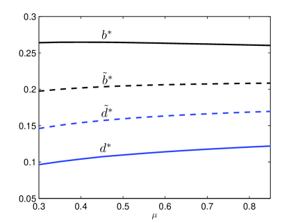
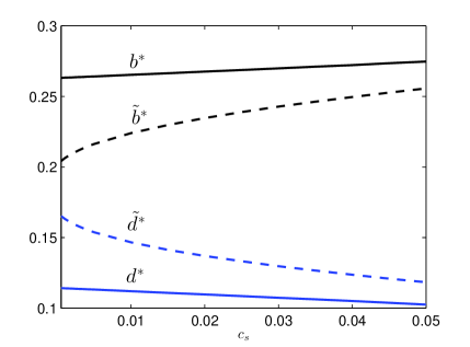
Figure 1: (Left) The optimal starting and stopping levels vs speed of mean reversion $\mu$. Parameters: $\sigma=0.15$, $\theta=0.2$, $r=0.05$, $c_{s}=0.001$, $c_{b}=0.001$. (Right) The optimal starting and stopping levels vs transaction cost $c_{s}$. Parameters: $\mu=0.6$, $\sigma=0.15$, $\theta=0.2$, $r=0.05$, $c_{b}=0.001$.

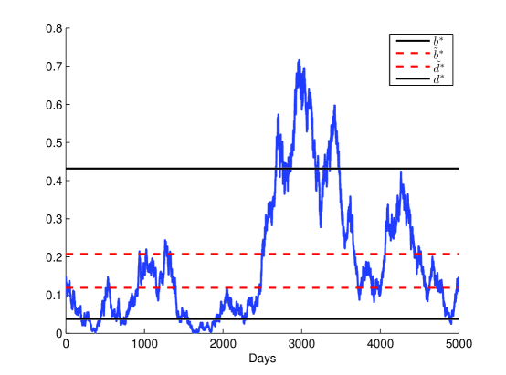
Figure 2: A sample CIR path, along with starting and stopping levels. Under the starting-stopping setting, a starting decision is made at $\nu_{d^{*}}=\inf\{t\geq 0:Y_{t}\leq d^{*}=0.0373\}$, and a stopping decision is made at $\tau_{b^{*}}=\inf\{t\geq\nu_{d^{*}}:Y_{t}\geq b^{*}=0.4316\}$. Under the optimal switching problem, entry and exit take place at $\nu_{\tilde{d}^{*}}=\inf\{t\geq 0:Y_{t}\leq\tilde{d}^{*}=0.1189\}$ , and $\tau_{\tilde{b}^{*}}=\inf\{t\geq\nu_{\tilde{d}^{*}}:Y_{t}\geq\tilde{b}^{*}=0.2078\}$ respectively. Parameters: $\mu=0.2$, $\sigma=0.3$, $\theta=0.2$, $r=0.05$, $c_{s}=0.001$, $c_{b}=0.001$.

4 Methods of Solution and Proofs

We now provide detailed proofs for our analytical results in Section 3 beginning with the optimal starting-stopping problem. Our main result here is Theorem 4.1 which provides a mathematical characterization of the value function, and establishes the optimality of our method of constructing the solution.

4.1 Optimal Starting-Stopping Problem

We first describe the general solution procedure for the stopping problem $V$, followed by the starting problem $J.$

4.1.1 Optimal Stopping Timing

A key step of our solution method involves the transformation

$$\phi(y):=-\frac{G(y)}{F(y)},\quad y\geq 0.$$ (4.1)

With this, we also define the function

$$H(z):=\begin{cases}\frac{h_{s}}{F}\circ\phi^{-1}(z)&\,\textrm{ if }\,z<0,\\ \lim_{z\to+\infty}\limits\frac{(h_{s}(y))^{+}}{F(y)}&\,\textrm{ if }\,z=0,\end{cases}$$ (4.2)

where $h_{s}$ is given in (2.4). We now prove the analytical form for the value function.

Theorem 4.1

Under the CIR model, the value function $V$ of (2.2) is given by

$$V(y)=F(y)W(\phi(y)),$$ (4.3)

with $F$ and $\phi$ given in (3.3) and (4.1) respectively, and $W$ is the decreasing smallest concave majorant of $H$ in (4.2).

Proof. We first show that $V(y)\geq F(y)W(\phi(y))$. Start at any $y\in[0,+\infty)$, we consider the first stopping time of $Y$ from an interval $[a,b]$ with $0\leq a\leq y\leq b\leq+\infty$. We compute the corresponding expected discounted reward

$$\mathbb{E}_{y}\{e^{-r(\tau_{a}\wedge\tau_{b})}h_{s}(Y_{\tau_{a}\wedge\tau_{b}})\} =h_{s}(a)\mathbb{E}_{y}\{e^{-r\tau_{a}}1{1}_{\{\tau_{a}<\tau_{b}\}}\}+h_{s}(b)\mathbb{E}_{y}\{e^{-r\tau_{b}}1{1}_{\{\tau_{a}>\tau_{b}\}}\}$$

$$=h_{s}(a)\frac{F(y)G(b)-F(b)G(y)}{F(a)G(b)-F(b)G(a)}+h_{s}(b)\frac{F(a)G(y)-F(y)G(a)}{F(a)G(b)-F(b)G(a)}$$

$$=F(y)\left[\frac{h_{s}(a)}{F(a)}\frac{\phi(b)-\phi(y)}{\phi(b)-\phi(a)}+\frac{h_{s}(b)}{F(b)}\frac{\phi(y)-\phi(a)}{\phi(b)-\phi(a)}\right]$$

$$=F(\phi^{-1}(z))\left[H(z_{a})\frac{z_{b}-z}{z_{b}-z_{a}}+H(z_{b})\frac{z-z_{a}}{z_{b}-z_{a}}\right],$$ (4.4)

where $z_{a}=\phi(a)$, $z_{b}=\phi(b)$. Since $V(y)\geq\sup_{\{a,b:a\leq y\leq b\}}\mathbb{E}_{y}\{e^{-r(\tau_{a}\wedge\tau_{b})}h_{s}(Y_{\tau_{a}\wedge\tau_{b}})\}$, we have

$$\frac{V(\phi^{-1}(z))}{F(\phi^{-1}(z))}\geq\sup_{\{z_{a},z_{b}:z_{a}\leq z\leq z_{b}\}}\left[H(z_{a})\frac{z_{b}-z}{z_{b}-z_{a}}+H(z_{b})\frac{z-z_{a}}{z_{b}-z_{a}}\right],$$ (4.5)

which implies that $V(\phi^{-1}(z))/F(\phi^{-1}(z))$ dominates the concave majorant of $H$.

Under the CIR model, the class of interval-type strategies does not include all single threshold-type strategies. In particular, the minimum value that $a$ can take is $0$. If $2\mu\theta<\sigma^{2}$, then $Y$ can reach level $0$ and reflects. The interval-type strategy with $a=0$ implies stopping the process $Y$ at level $0$, even though it could be optimal to wait and let $Y$ evolve.

Hence, we must also consider separately the candidate strategy of waiting for $Y$ to reach an upper level $b\geq y$ without a lower stopping level. The well-known supermartingale property of $(e^{-rt}V(Y_{t}))_{t\geq 0}$ (see Appendix D of Karatzas and Shreve (1998)) implies that $V(y)\geq\mathbb{E}_{y}\{e^{-r\tau}V(Y_{\tau})\}$ for $\tau\in{\mathcal{T}}$. Then, taking $\tau=\tau_{b}$, we have

$$V(y)\geq\mathbb{E}_{y}\{e^{-r\tau_{b}}V(Y_{\tau_{b}})\}=V(b)\frac{F(y)}{F(b)},$$

or equivalently,

$$\frac{V(\phi^{-1}(z))}{F(\phi^{-1}(z))}=\frac{V(y)}{F(y)}\geq\frac{V(b)}{F(b)}=\frac{V(\phi^{-1}(z_{b}))}{F(\phi^{-1}(z_{b}))},$$ (4.6)

which indicates that $V(\phi^{-1}(z))/F(\phi^{-1}(z))$ is decreasing. By (4.5) and (4.6), we now see that $V(y)\geq F(y)W(\phi(y))$, where $W$ is the decreasing smallest concave majorant of $H$.

For the reverse inequality, we first show that

$$F(y)W(\phi(y))\geq\mathbb{E}_{y}\{e^{-r(t\wedge\tau)}F(Y_{t\wedge\tau})W(\phi(Y_{t\wedge\tau}))\},$$ (4.7)

for $y\in[0,+\infty)$, $\tau\in{\mathcal{T}}$ and $t\geq 0$. If the initial value $y=0$, then the decreasing property of $W$ implies the inequality

$$\mathbb{E}_{0}\{e^{-r({t\wedge\tau})}F(Y_{t\wedge\tau})W(\phi(Y_{t\wedge\tau}))\}\leq\mathbb{E}_{0}\{e^{-r(t\wedge\tau)}F(Y_{t\wedge\tau})\}W(\phi(0))=F(0)W(\phi(0)),$$ (4.8)

where the equality follows from the martingale property of $(e^{-rt}F(Y_{t}))_{t\geq 0}$.

When $y>0$, the concavity of $W$ implies that, for any fixed $z$, there exists an affine function $L_{z}(\alpha):=m_{z}\alpha+c_{z}$ such that $L_{z}(\alpha)\geq W(\alpha)$ for $\alpha\geq\phi(0)$ and $L_{z}(z)=W(z)$ at $\alpha=z$, with constants $m_{z}$ and $c_{z}$. In turn, this yields the inequality

$$\mathbb{E}_{y} \{e^{-r(\tau_{0}\wedge t\wedge\tau)}F(Y_{\tau_{0}\wedge t\wedge\tau})W(\phi(Y_{\tau_{0}\wedge t\wedge\tau}))\}$$ (4.9)

$$\leq\mathbb{E}_{y}\{e^{-r(\tau_{0}\wedge t\wedge\tau)}F(Y_{\tau_{0}\wedge t\wedge\tau})L_{\phi(y)}(\phi(Y_{\tau_{0}\wedge t\wedge\tau}))\}$$

$$=m_{\phi(y)}\mathbb{E}_{y}\{e^{-r(\tau_{0}\wedge t\wedge\tau)}F(Y_{\tau_{0}\wedge t\wedge\tau})\phi(Y_{\tau_{0}\wedge t\wedge\tau})\}+c_{\phi(y)}\mathbb{E}_{y}\{e^{-r(\tau_{0}\wedge t\wedge\tau)}F(Y_{\tau_{0}\wedge t\wedge\tau})\}$$

$$=-m_{\phi(y)}\mathbb{E}_{y}\{e^{-r(\tau_{0}\wedge t\wedge\tau)}G(Y_{\tau_{0}\wedge t\wedge\tau})\}+c_{\phi(y)}\mathbb{E}_{y}\{e^{-r(\tau_{0}\wedge t\wedge\tau)}F(Y_{\tau_{0}\wedge t\wedge\tau})\}$$

$$=-m_{\phi(y)}G(y)+c_{\phi(y)}F(y)$$ (4.10)

$$=F(y)L_{\phi(y)}(\phi(y))$$

$$=F(y)W(\phi(y)),$$ (4.11)

where $\eqref{2}$ follows from the martingale property of $(e^{-rt}F(Y_{t}))_{t\geq 0}$ and $(e^{-rt}G(Y_{t}))_{t\geq 0}$. If $2\mu\theta\geq\sigma^{2}$, then $\tau_{0}=+\infty$ for $y>0$. This immediately reduces (4.9)-(4.11) to the desired inequality (4.7).

On the other hand, if $2\mu\theta<\sigma^{2}$, then we decompose (4.9) into two terms:

$$\mathbb{E}_{y}\{e^{-r(\tau_{0}\wedge t\wedge\tau)}F(Y_{\tau_{0}\wedge t\wedge\tau})W(\phi(Y_{\tau_{0}\wedge t\wedge\tau}))\}$$

$$=\underbrace{\mathbb{E}_{y}\{e^{-r(t\wedge\tau)}F(Y_{t\wedge\tau})W(\phi(Y_{t\wedge\tau}))1{1}_{\{t\wedge\tau\leq\tau_{0}\}}\}}_{\text{(I)}}+\underbrace{\mathbb{E}_{y}\{e^{-r\tau_{0}}F(Y_{\tau_{0}})W(\phi(Y_{\tau_{0}}))1{1}_{\{t\wedge\tau>\tau_{0}\}}\}}_{\text{(II)}}.$$ (4.12)

By the optional sampling theorem and decreasing property of $W$, the second term satisfies

(II) $$=W(\phi(0))\mathbb{E}_{y}\{e^{-r\tau_{0}}F(Y_{\tau_{0}})1{1}_{\{t\wedge\tau>\tau_{0}\}}\}$$

$$\geq W(\phi(0))\mathbb{E}_{y}\{e^{-r(t\wedge\tau)}F(Y_{t\wedge\tau})1{1}_{\{t\wedge\tau>\tau_{0}\}}\}$$

$$\geq\mathbb{E}_{y}\{e^{-r(t\wedge\tau)}F(Y_{t\wedge\tau})W(\phi(Y_{t\wedge\tau}))1{1}_{\{t\wedge\tau>\tau_{0}\}}\}=:\text{(II')}.$$ (4.13)

Combining (4.13) with (4.11), we arrive at

$$F(y)W(\phi(y))\geq\text{(I)}+\text{(II')}=\mathbb{E}_{y}\{e^{-r(t\wedge\tau)}F(Y_{t\wedge\tau})W(\phi(Y_{t\wedge\tau}))\},$$

for all $y>0$. In all, inequality (4.7) holds for all $y\in[0,+\infty)$, $\tau\in{\mathcal{T}}$ and $t\geq 0$. From (4.7) and the fact that $W$ majorizes $H$, it follows that

$$F(y)W(\phi(y)) \geq\mathbb{E}_{y}\{e^{-r(t\wedge\tau)}F(Y_{t\wedge\tau})W(\phi(Y_{t\wedge\tau}))\}$$ (4.14)

$$\geq\mathbb{E}_{y}\{e^{-r(t\wedge\tau)}F(Y_{t\wedge\tau})H(\phi(Y_{t\wedge\tau}))\}\geq\mathbb{E}_{y}\{e^{-r(t\wedge\tau)}h_{s}(Y_{t\wedge\tau})\}.$$ (4.15)

Maximizing (4.15) over all $\tau\in{\mathcal{T}}$ and $t\geq 0$ yields the reverse inequality $F(y)W(\phi(y))\geq V(y)$.   

In summary, we have found an expression for the value function $V(y)$ in (4.3), and proved that it is sufficient to consider only candidate stopping times described by the first time $Y$ reaches a single upper threshold or exits an interval. To determine the optimal timing strategy, we need to understand the properties of $H$ and its smallest concave majorant $W$. To this end, we have the following lemma.

Lemma 4.2

The function $H$ is continuous on $[\phi(0),0]$, twice differentiable on $(\phi(0),0)$ and possesses the following properties:

1. $H(0)=0$, and

   $$H(z)\begin{cases}<0&\,\textrm{ if }\,z\in[\phi(0),\phi(c_{s})),\\ >0&\,\textrm{ if }\,z\in(\phi(c_{s}),0).\end{cases}$$ (4.16)

2. $H(z)$ is strictly increasing for $z\in(\phi(0),\phi(c_{s})\vee\phi(y_{s}))$.

3. $$H(z)\textrm{ is }\begin{cases}\textrm{convex}&\,\textrm{ if }\,z\in(\phi(0),\phi(y_{s})],\\ \textrm{concave}&\,\textrm{ if }\,z\in[\phi(y_{s}),0).\end{cases}$$

In Figure 3, we see that $H$ is first increasing then decreasing, and first convex then concave. Using these properties, we now derive the optimal stopping timing.

(a) $2\mu\theta<\sigma^{2}$

(b) $2\mu\theta\geq\sigma^{2}$

Figure 3: Sketches of $H$ and $W$. The function $W$ is equal to the constant $H(z^{*})$ on $(\phi(0),z^{*})$, and coincides with $H$ on $[z^{*},0]$. Note that $-\infty\!<\!\phi(0)\!<\!0$ if $2\mu\theta<\sigma^{2}$, and $\phi(0)\!=\!-\infty$ if $2\mu\theta\geq\sigma^{2}$.

Proof of Theorem 3.1

We determine the value function in the form: $V(y)=F(y)W(\phi(y))$, where $W$ is the decreasing smallest concave majorant of $H$. By Lemma 4.2 and Figure 3, $H$ peaks at $z^{*}>\phi(c_{s})\vee\phi(y_{s})$ so that

$${H}^{\prime}\!(z^{*})=0.$$ (4.17)

In turn, the decreasing smallest concave majorant admits the form:

$$W(z)=\begin{cases}H(z^{*})&\,\textrm{ if }\,z<z^{*},\\ H(z)&\,\textrm{ if }\,z\geq z^{*}.\end{cases}$$ (4.18)

Substituting $b^{*}=\phi^{-1}(z^{*})$ into (4.17), we have

$${H}^{\prime}\!(z^{*}) =\frac{F(\phi^{-1}(z^{*}))-(\phi^{-1}(z^{*})-c_{s}){F}^{\prime}\!(\phi^{-1}(z^{*}))}{{F}^{\prime}\!(\phi^{-1}(z^{*}))G(\phi^{-1}(z^{*}))-F(\phi^{-1}(z^{*})){G}^{\prime}\!(\phi^{-1}(z^{*}))}$$

$$=\frac{F(b^{*})-(b^{*}-c_{s}){F}^{\prime}\!(b^{*})}{{F}^{\prime}\!(b^{*})G(b^{*})-F(b^{*}){G}^{\prime}\!(b^{*})},$$

which can be further simplified to (3.7). We can express $H(z^{*})$ in terms of $b^{*}$:

$$H(z^{*})=\frac{b^{*}-c_{s}}{F(b^{*})}.$$ (4.19)

Applying (4.19) to (4.18), we get

$$W(\phi(y))=\begin{cases}H(z^{*})=\frac{b^{*}-c_{s}}{F(b^{*})}&\,\textrm{ if }\,y<b^{*},\\ H(\phi(y))=\frac{y-c_{s}}{F(y)}&\,\textrm{ if }\,y\geq b^{*}.\end{cases}$$

Finally, substituting this into the value function $V(y)=F(y)W(\phi(y))$, we conclude.

4.1.2 Optimal Starting Timing

We now turn to the optimal starting problem. Our methodology in Section 4.1.1 applies to general payoff functions, and thus can be applied to the optimal starting problem (2.3) as well. To this end, we apply the same transformation (4.1) and define the function

$$\hat{H}(z):=\begin{cases}\frac{\hat{h}}{F}\circ\phi^{-1}(z)&\,\textrm{ if }\,z<0,\\ \lim_{y\to+\infty}\limits\frac{(\hat{h}(y))^{+}}{F(y)}&\,\textrm{ if }\,z=0,\end{cases}$$

where $\hat{h}$ is given in (3.8). We then follow Theorem 3.1 to determine the value function $J$. This amounts to finding the decreasing smallest concave majorant $\hat{W}$ of $\hat{H}$. Indeed, we can replace $H$ and $W$ with $\hat{H}$ and $\hat{W}$ in Theorem 3.1 and its proof. As a result, the value function of the optimal starting timing problem must take the form

$$J(y)=F(y)\hat{W}(\phi(y)).$$

To solve the optimal starting timing problem, we need to understand the properties of $\hat{H}$.

Lemma 4.3

The function $\hat{H}$ is continuous on $[\phi(0),0]$, differentiable on $(\phi(0),0)$, and twice differentiable on $(\phi(0),\phi(b^{*}))\cup(\phi(b^{*}),0)$, and possesses the following properties:

1. $\hat{H}(0)=0$. Let $\bar{d}$ denote the unique solution to $\hat{h}(y)=0$, then $\bar{d}<b^{*}$ and

   $$\hat{H}(z)\begin{cases}>0&\,\textrm{ if }\,z\in[\phi(0),\phi(\bar{d})),\\ <0&\,\textrm{ if }\,z\in(\phi(\bar{d}),0).\end{cases}$$

2. $\hat{H}(z)$ is strictly increasing for $z>\phi(b^{*})$ and $\lim_{z\to\phi(0)}\hat{H}^{{}^{\prime}}\!(z)=0$.

3. $$\hat{H}(z)\textrm{ is }\begin{cases}\textrm{concave}&\,\textrm{ if }\,z\in(\phi(0),\phi(y_{b})),\\ \textrm{convex}&\,\textrm{ if }\,z\in(\phi(y_{b}),0).\end{cases}$$

By Lemma 4.3, we sketch $\hat{H}$ in Figure 4.

(a) $2\mu\theta<\sigma^{2}$

(b) $2\mu\theta\geq\sigma^{2}$

Figure 4: Sketches of $\hat{H}$ and $\hat{W}$. The function $\hat{W}$ coincides with $\hat{H}$ on $[\phi(0),\hat{z}]$ and is a straight line tangent to $\hat{H}$ at $\hat{z}$ on $(\hat{z},0]$. Note that $-\infty\!<\!\phi(0)\!<\!0$ if $2\mu\theta<\sigma^{2}$, and $\phi(0)\!=\!-\infty$ if $2\mu\theta\geq\sigma^{2}$.

Proof of Theorem 3.2

To determine the value function in the form: $J(y)=F(y)\hat{W}(\phi(y))$, we analyze the decreasing smallest concave majorant, $\hat{W}$, of $\hat{H}$. By Lemma 4.3 and Figure 3, we have $\hat{H}^{{}^{\prime}}\!(z)\to 0$ as $z\to\phi(0)$. Therefore, there exists a unique number $\hat{z}\in(\phi(0),\phi(b^{*}))$ such that

$$\frac{\hat{H}(\hat{z})}{\hat{z}}=\hat{H}^{{}^{\prime}}\!(\hat{z}).$$ (4.20)

In turn, the decreasing smallest concave majorant admits the form:

$$\hat{W}(z)=\begin{cases}\hat{H}(z)&\,\textrm{ if }\,z\leq\hat{z},\\ z\frac{\hat{H}(\hat{z})}{\hat{z}}&\,\textrm{ if }\,z>\hat{z}.\end{cases}$$ (4.21)

Substituting $d^{*}=\phi^{-1}(\hat{z})$ into (4.20), we have

$$\frac{\hat{H}(\hat{z})}{\hat{z}}=\frac{\hat{H}(\phi(d^{*})}{\phi(d^{*})}=-\frac{V(d^{*})-d^{*}-c_{b}}{G(d^{*})},$$ (4.22)

and

$$\hat{H}^{{}^{\prime}}\!(\hat{z})=\frac{F(d^{*})({V}^{\prime}\!(d^{*})-1)-F^{{}^{\prime}}\!(d^{*})(V(d^{*})-(d^{*}+c_{b}))}{F^{{}^{\prime}}\!(d^{*})G(d^{*})-F(d^{*})G^{{}^{\prime}}\!(d^{*})}.$$

Equivalently, we can express condition (4.20) in terms of $d^{*}$:

$$-\frac{V(d^{*})-(d^{*}+c_{b})}{G(d^{*})}=\frac{F(d^{*})({V}^{\prime}\!(d^{*})-1)-F^{{}^{\prime}}\!(d^{*})(V(d^{*})-(d^{*}+c_{b}))}{F^{{}^{\prime}}\!(d^{*})G(d^{*})-F(d^{*})G^{{}^{\prime}}\!(d^{*})},$$

which shows $d^{*}$ satisfies (3.11) after simplification.

Applying (4.22) to (4.21), we get

$$W(\phi(y))=\begin{cases}\hat{H}(\phi(y))=\frac{V(y)-(y+c_{b})}{F(y)}&\,\textrm{ if }\,y\in[0,d^{*}],\\ \phi(y)\frac{\hat{H}(\hat{z})}{\hat{z}}=\frac{V(d^{*})-(d^{*}+c_{b})}{G(d^{*})}\frac{G(y)}{F(y)}&\,\textrm{ if }\,y\in(d^{*},+\infty).\end{cases}$$

From this, we obtain the value function.

4.2 Optimal Switching Problem

Proofs of Theorems 3.3 and 3.4

Zervos et al. (2013) have studied a similar problem of trading a mean-reverting asset with fixed transaction costs, and provided detailed proofs using a variational inequalities approach. In particular, we observe that $y_{b}$ and $y_{s}$ in (3.4) play the same roles as $x_{b}$ and $x_{s}$ in Assumption 4 in Zervos et al. (2013), respectively. However, Assumption 4 in Zervos et al. (2013) requires that $0\leq x_{b},$ this is not necessarily true for $y_{b}$ in our problem. We have checked and realized that this assumption is not necessary for Theorem 3.3, and that $y_{b}<0$ simply implies that there is no optimal starting level, i.e. it is never optimal to start.

In addition, Zervos et al. (2013) assume (in their Assumption 1) that the hitting time of level $0$ is infinite with probability 1. In comparison, we consider not only the CIR case where 0 is inaccessible, but also when the CIR process has a reflecting boundary at $0$. In fact, we find that the proofs in Zervos et al. (2013) apply to both cases under the CIR model. Therefore, apart from relaxation of the aforementioned assumptions, the proofs of our Theorems 3.3 and 3.4 are the same as that of Lemmas 1 and 2 in Zervos et al. (2013) respectively.

Appendix A Appendix

A.4  Proof of Lemma 4.2 (Properties of $H$).  (i) First, we compute

$$H(0)=\lim_{y\to+\infty}\frac{(h_{s}(y))^{+}}{F(y)}=\lim_{y\to+\infty}\frac{y-c_{s}}{F(x)}=\lim_{y\to+\infty}\frac{1}{{F}^{\prime}\!(y)}=0.$$

Using the facts that $F(y)>0$ and $\phi(y)$ is a strictly increasing function, (4.16) follows.

(ii) We look at the first derivative of $H$:

$${H}^{\prime}\!(z)=\frac{1}{\phi^{\prime}(y)}(\frac{h_{s}}{F})^{\prime}(y)=\frac{1}{\phi^{\prime}(y)}\frac{F(y)-(y-c_{s}){F}^{\prime}\!(y)}{{F}^{2}(y)},\quad z=\phi(y).$$

Since both $\phi^{\prime}(y)$ and ${F}^{2}(y)$ are positive, it remains to determine the sign of $F(y)-(y-c_{s}){F}^{\prime}\!(y)$. Since ${F}^{\prime}\!(y)>0$, we can equivalently check the sign of $v(y):=\frac{F(y)}{{F}^{\prime}\!(y)}-(y-c_{s})$. Note that $v^{\prime}(y)=-\frac{F(y){F}^{\prime\prime}\!(y)}{({F}^{\prime}\!(y))^{2}}<0$. Therefore, $v(y)$ is a strictly decreasing function. Also, it is clear that $v(c_{s})>0$ and $v(y_{s})>0$. Consequently, $v(y)>0$ if $y<(c_{s}\vee y_{s})$ and hence, $H(z)$ is strictly increasing if $z\in(\phi(0),\phi(c_{s})\vee\phi(y_{s}))$.

(iii) By differentiation, we have

$$H^{{}^{\prime\prime}}\!(z)=\frac{2}{\sigma^{2}F(y)(\phi^{\prime}(y))^{2}}({\mathcal{L}}-r)h_{s}(y),\quad z=\phi(y).$$

Since $\sigma^{2},F(y)$ and $(\phi^{\prime}(y))^{2}$ are all positive, the convexity/concavity of $H^{{}^{\prime\prime}}$ depends on the sign of

$$({\mathcal{L}}-r)h_{s}(y)=\mu(\theta-y)-r(y-c_{s})=(\mu\theta+rc_{s})-(\mu+r)y \begin{cases}\geq 0&\,\textrm{ if }\,y\in[0,y_{s}],\\ \leq 0&\,\textrm{ if }\,y\in[y_{s},+\infty),\end{cases}$$

which implies property (iii). $\scriptstyle{\blacksquare}$

A.5  Proof of Lemma 4.3 (Properties of $\hat{H}$).  It is straightforward to check that $V(y)$ is continuous and differentiable everywhere, and twice differentiable everywhere except at $y=b^{*}$, and all these holds for $\hat{h}(y)=V(y)-(y+c_{b})$. Both $F$ and $\phi$ are twice differentiable. In turn, the continuity and differentiability of $\hat{H}$ on $(\phi(0),0)$ and twice differentiability of $\hat{H}$ on $(\phi(0),\phi(b^{*}))\cup(\phi(b^{*}),0)$ follow.

To show the continuity of $\hat{H}$ at $0$, we note that

$$\hat{H}(0) =\lim_{y\to+\infty}\frac{(\hat{h}(y))^{+}}{F(y)}=\lim_{y\to+\infty}\frac{0}{F(y)}=0,\quad\text{ and }$$

$$\lim_{z\rightarrow 0}\hat{H}(z) =\lim_{y\to+\infty}\frac{\hat{h}}{F}(y)=\lim_{y\to+\infty}\frac{-(c_{s}+c_{b})}{F(y)}=0.$$

From this, we conclude that $\hat{H}$ is also continuous at $0$.

(i) First, for $y\in[b^{*},+\infty)$, $\hat{h}(y)\equiv-(c_{s}+c_{b})$. For $y\in(0,b^{*})$, we compute

$${V}^{\prime}\!(y)=\frac{b^{*}-c_{s}}{F(b^{*})}{F}^{\prime}\!(y)=\frac{{F}^{\prime}\!(y)}{{F}^{\prime}\!(b^{*})},\quad\textrm{by \eqref{eq:solvebCIR}}.$$

Recall that ${F}^{\prime}\!(y)$ is a strictly increasing function and $\hat{h}(y)=V(y)-y-c_{b}$. Differentiation yields

$$\hat{h}^{{}^{\prime}}\!(y)={V}^{\prime}\!(y)-1=\frac{{F}^{\prime}\!(y)}{{F}^{\prime}\!(b^{*})}-1<\frac{{F}^{\prime}\!(b^{*})}{{F}^{\prime}\!(b^{*})}-1=0,\quad y\in(0,b^{*}),$$

which implies that $\hat{h}(y)$ is strictly decreasing for $y\in(0,b^{*})$. On the other hand, $\hat{h}(0)>0$ as we are considering the non-trivial case. Therefore, there exists a unique solution $\bar{d}<b^{*}$ to $\hat{h}(y)=0$, such that $\hat{h}(y)>0$ for $y\in[0,\bar{d})$, and $\hat{h}(y)<0$ for $y\in(\bar{d},+\infty)$. With $\hat{H}(z)=(\hat{h}/F)\circ\phi^{-1}(z)$, the above properties of $\hat{h}$, along with the facts that $\phi(y)$ is strictly increasing and $F(y)>0$, imply property (i).

(ii)With $z=\phi(y)$, for $y>b^{*}$, $\hat{H}(z)$ is strictly increasing since

$$\hat{H}^{{}^{\prime}}\!(z)=\frac{1}{\phi^{\prime}(y)}(\frac{\hat{h}}{F})^{\prime}(y)=\frac{1}{\phi^{\prime}(y)}(\frac{-(c_{s}+c_{b})}{F(y)})^{\prime}=\frac{1}{\phi^{\prime}(y)}\frac{(c_{s}+c_{b})F^{{}^{\prime}}\!(y)}{F^{\chi^{2}}(y)}>0.$$

When $y\to 0$, because $(\frac{\hat{h}(y)}{F(y)})^{\prime}$ is finite, but $\phi^{\prime}(y)\to+\infty$, we have $\lim_{z\to\phi(0)}\hat{H}^{{}^{\prime}}\!(z)=0$.

(iii) Consider the second derivative:

$$\hat{H}^{{}^{\prime\prime}}\!(z)=\frac{2}{\sigma^{2}F(y)(\phi^{\prime}(y))^{2}}({\mathcal{L}}-r)\hat{h}(y).$$

The positivities of $\sigma^{2},F(y)$ and $(\phi^{\prime}(y))^{2}$ suggest that we inspect the sign of $({\mathcal{L}}-r)\hat{h}(y)$:

$$({\mathcal{L}}-r)\hat{h}(y) =\frac{1}{2}\sigma^{2}x{V}^{\prime\prime}\!(y)+\mu(\theta-y){V}^{\prime}\!(y)-\mu(\theta-y)-r(V(y)-(y+c_{b}))$$

$$=\begin{cases}(\mu+r)y-\mu\theta+rc_{b}&\,\textrm{ if }\,y<b^{*},\\ r(c_{s}+c_{b})>0&\,\textrm{ if }\,y>b^{*}.\end{cases}$$

Since $\mu,r>0$ by assumption, $({\mathcal{L}}-r)\hat{h}(y)$ is strictly increasing on $(0,b^{*})$. Next, we show that $0\!<\!y_{b}\!<\!y_{s}\!<\!b^{*}$. By the fact that ${F}^{\prime}\!(0)=\frac{r}{\mu\theta}$ and the assumption that $V(0)=\frac{b^{*}-c_{s}}{F(b^{*})}>c_{b}$, we have

$${V}^{\prime}\!(0)=\frac{b^{*}-c_{s}}{F(b^{*})}{F}^{\prime}\!(0)=\frac{b^{*}-c_{s}}{F(b^{*})}\frac{r}{\mu\theta}>\frac{rc_{b}}{\mu\theta}.$$

In addition, by the convexity of $V$ and ${V}^{\prime}\!(b^{*})=1$, it follows that

$$\frac{rc_{b}}{\mu\theta}<{V}^{\prime}\!(0)<{V}^{\prime}\!(b^{*})=1,$$

which implies $\mu\theta>rc_{b}$ and hence $y_{b}>0$. By simply comparing the definitions of $y_{b}$ and $y_{s}$, it is clear that $y_{b}<y_{s}$. Therefore, by observing that $({\mathcal{L}}-r)\hat{h}(y_{b})=0$, we conclude $({\mathcal{L}}-r)\hat{h}(y)<0$ if $y\in[0,y_{b})$, and $({\mathcal{L}}-r)\hat{h}(y)>0$ if $y\in(y_{b},+\infty)$. This suggests the concavity and convexity of $\hat{H}$ as desired. $\scriptstyle{\blacksquare}$

References

• Abramowitz and Stegun (1965) Abramowitz, M. and Stegun, I. (1965). Handbook of Mathematical Functions: with Formulas, Graphs, and Mathematical Tables, volume 55. Dover Publications.
• Bensoussan and Lions (1982) Bensoussan, A. and Lions, J.-L. (1982). Applications of Variational Inequalities in Stochastic Control. North-Holland Publishing Co., Amsterdam.
• Borodin and Salminen (2002) Borodin, A. and Salminen, P. (2002). Handbook of Brownian Motion: Facts and Formulae. Birkhauser, 2nd edition.
• Carmona and León (2007) Carmona, J. and León, A. (2007). Investment option under CIR interest rates. Finance Research Letters, 4(4):242–253.
• Cox et al. (1985) Cox, J. C., Ingersoll, J. E., and Ross, S. A. (1985). A theory of the term structure of interest rates. Econometrica, 53(2):385–408.
• Dayanik and Karatzas (2003) Dayanik, S. and Karatzas, I. (2003). On the optimal stopping problem for one-dimensional diffusions. Stochastic Processes and Their Applications, 107(2):173–212.
• Dixit (1994) Dixit, A. K. (1994). Investment Under Uncertainty. Princeton University Press.
• Dynkin and Yushkevich (1969) Dynkin, E. and Yushkevich, A. (1969). Markov Processes: Theorems and Problems. Plenum Press.
• Ewald and Wang (2010) Ewald, C.-O. and Wang, W.-K. (2010). Irreversible investment with Cox-Ingersoll-Ross type mean reversion. Mathematical Social Sciences, 59(3):314–318.
• Feller (1951) Feller, W. (1951). Two singular diffusion problems. The Annals of Mathematics, 54(1):173–182.
• Göing-Jaeschke and Yor (2003) Göing-Jaeschke, A. and Yor, M. (2003). A survey and some generalizations of Bessel processes. Bernoulli, 9(2):313–349.
• Heston (1993) Heston, S. L. (1993). A closed form solution for options with stochastic volatility with applications to bond and currency options. review of financial studies, 6:327–343.
• Karatzas and Shreve (1998) Karatzas, I. and Shreve, S. (1998). Methods of Mathematical Finance. Springer, New York.
• Karlin and Taylor (1981) Karlin, S. and Taylor, H. M. (1981). A Second Course in Stochastic Processes, volume 2. Academic Press.
• Karpowicz and Szajowski (2007) Karpowicz, A. and Szajowski, K. (2007). Double optimal stopping of a risk process. Stochastics: An International Journal of Probability and Stochastics Processes, 79(1-2):155–167.
• Lebedev (1972) Lebedev, N. (1972). Special Functions & Their Applications. Dover Publications.
• Leung and Li (2014) Leung, T. and Li, X. (2014). Optimal mean reversion trading with transaction cost and stop-loss exit. Working paper, Columbia University.
• Leung et al. (2014) Leung, T., Li, X., and Wang, Z. (2014). Optimal multiple trading times under the exponential OU model with transaction costs. Working paper, Columbia University.
• Leung and Liu (2012) Leung, T. and Liu, P. (2012). Risk premia and optimal liquidation of credit derivatives. International Journal of Theoretical & Applied Finance, 15(8).
• Menaldi et al. (1996) Menaldi, J., Robin, M., and Sun, M. (1996). Optimal starting-stopping problems for Markov-Feller processes. Stochastics: An International Journal of Probability and Stochastic Processes, 56(1-2):17–32.
• Øksendal (2003) Øksendal, B. (2003). Stochastic Differential Equations: an Introduction with Applications. Springer.
• Ribeiro and Hodges (2004) Ribeiro, D. R. and Hodges, S. D. (2004). A two-factor model for commodity prices and futures valuation. Working paper, University of Warwick.
• Shiryaev et al. (2008) Shiryaev, A., Xu, Z., and Zhou, X. (2008). Thou shalt buy and hold. Quantitative Finance, 8(8):765–776.
• Sun (1992) Sun, M. (1992). Nested variational inequalities and related optimal starting-stopping problems. Journal of Applied Probability, 29(1):104–115.
• Tanaka (1993) Tanaka, T. (1993). On two-parameter discrete time optimal starting-stopping problems. Nihonkai Mathematical Journal, 4(1):17–34.
• Zervos et al. (2013) Zervos, M., Johnson, T., and Alazemi, F. (2013). Buy-low and sell-high investment strategies. Mathematical Finance, 23(3):560–578.