IPMU-14-0343

ICRR-Report-695-2014-21

Coupling Unification and Dark Matter in a Standard Model Extension with Adjoint Majorana Fermions

Tasuku Aizawa^(a), Masahiro Ibe^(a,b), and Kunio Kaneta^(a)

^(a)Institute for Cosmic Ray Research (ICRR), Theory Group,
University of Tokyo, Kashiwa, Chiba 277-8568, Japan
^(b)Kavli Institute for the Physics and Mathematics of the Universe (IPMU),
University of Tokyo, Kashiwa, Chiba 277-8583, Japan

1 Introduction

After the discovery of the Higgs boson at the LHC experiments [1], the Standard Model (SM) was fully established as the unified theory of the weak and electromagnetic interactions. With the success of the unified electroweak theory, it is worthy to reappraise the long-sought idea, the grand unified theory (GUT) [2] (for a review see e.g. [3]). The GUT has served as a guiding principle for theories beyond the Standard Model where the three gauge coupling constants in the SM are unified into a universal gauge coupling constant at a very high energy scale, i.e. the unification scale [4]. As is well known, however, the naive extrapolations of the three gauge coupling constants towards the high energy scale do not meet very precisely at a single scale [5, 6, 7]. Therefore, the ideas of the GUT inevitably require new charged particles with masses above the electroweak scale but below the unification scale.

Along with the GUT, dark matter has been another no less important guiding principle for theories beyond the SM. In fact, the cold dark matter paradigm is a pillar of modern cosmology, whose existence has been established by numerous cosmological and astrophysical observations on a wide range of scales. Although its detailed nature has remained unknown, we are almost certain that dark matter is not a part of the SM, and hence, its identification is the most important challenge in cosmology, astrophysics, and particle physics (for reviews, see e.g. [8, 9, 10]).

For decades, these two principles have served as important criteria for assessing how attractive a model of beyond the SM is. For example, these two guiding principles are beautifully satisfied in the minimal supersymmetric Standard Model (MSSM). With these successes, the MSSM remains one of the leading candidates of the theory beyond the SM, despite the fact that the relatively large Higgs boson mass at around 125–126 GeV and the null observations of the predicted superparticles seem to diminish one of the motivations of the MSSM, naturalness of the electroweak scale.

To achieve a model with a dark matter candidate and a precise unification simultaneously, however, we do not need a large extension of the SM as in the case of the MSSM, but it is possible with much smaller extensions. For example, a smaller extension of the SM with only two Majorana Fermions in the adjoint representations of $SU(2)_{L}$ and $SU(3)_{c}$ gauge groups of the SM is enough to achieved a precise coupling unification along with a good candidate for dark matter [11], where their masses are required to be in the multi-TeV range and in the intermediate scale, respectively. Since the $SU(2)_{L}$ triplet Majorana fermion is predicted to be around the TeV scale, the model is consistent with the so-called thermal “minimal dark matter scenario” [21] where the relic density of the thermally produced triplet fermion is consistent with the observation for its mass being $3$ TeV [22, 21].

In this paper, we revisit this small extension of the SM with the adjoint fermions as a low-energy effective theory below the GUT scale. In particular, we discuss the non-thermal production of the triplet dark matter from the decay of the thermally produced octet fermions whose mass is at around $10^{10-11}$ GeV. As we will show, the non-thermal contribution to the dark matter density dominates over the thermal contribution when the octet fermion decays through the higher dimensional operators suppressed by the GUT scale. In such cases, the lighter triplet fermion than $3$ TeV can also be a viable candidate for dark matter. Due to the lighter mass of the triplet fermions, the model is more testable than the thermal minimal dark matter scenario in [21]. We also discuss how the dark matter mass is correlated to the proton lifetime predicted in the GUT models.

The organisation of the paper is as follows. In section 2, we briefly review the small extension of the SM with adjoint Majorana fermions which allows a precise unification of the three gauge coupling constants at a high energy scale. In section 3, we discuss the non-thermal production of the triplet fermion from the decay of the thermally produced octet fermion. There, we show that the non-thermally produced dark matter explains the observed dark matter density. In section 4, we discuss the proton lifetime in this model. The final section is devoted to our conclusions.

2 Coupling Unification and Masses of Adjoint Fermions

Let us briefly summarize the small extension of the SM with adjoint Majorana fermions. In the following, we name the $SU(2)_{L}$ triplet and the $SU(3)_{c}$ octet Majorana fermions, the wino-like fermion ($\tilde{w}$) and the gluino-like fermion ($\tilde{g}$), respectively, after the fashion of the MSSM. Here, we discuss the masses of the adjoint fermions which allows a successful unification. In this paper, we assume the minimal gauge group of the GUT to be $SU(5)$, where the leptons and quarks are unified into the $\bar{\bf 5}$ and $\bf 10$ representations respectively [3].

To see how the three gauge coupling constants are extrapolated at high energy scales, let us consider the renormalization group equations,

$$\frac{d\alpha_{a}^{-1}}{d\ln\mu}=\frac{b_{a}}{2\pi}\ ,\,\,\,(a=1,2,3)\ ,$$ (1)

where $\mu$ is the renormalization scale, and $\alpha_{a}=g_{a}^{2}/4\pi$ with $g_{a}$’s being the three gauge coupling constants of the SM. The parameters $b_{a}$’s are so-called the coefficients of the beta functions. Since we are assuming the GUT with the $SU(5)$ gauge group, we use the rescaled gauge coupling of the $U(1)_{Y}$ gauge interaction, i.e. $g_{1}=\sqrt{5/3}\,g^{\prime}$,

If the SM is an effective low energy theory of a GUT realized at a very high energy scale (the GUT scale), it is expected that the three gauge coupling constants meet together at around the GUT scale. As is well known, however, the extrapolation of the SM gauge coupling constants shows two failures of the SM as a low energy effective of a GUT;

• The coupling constants do not unify at a single scale, and hence, the unification is not precise at all.

• If we take $g_{1}-g_{2}$ unification scale or $g_{1}-g_{3}$ unification scale as the GUT scale which are at around $10^{13-14}$ GeV, the predicted proton lifetime is too small to be consistent with the experimental constraints.

To circumvent these failures, we immediately find that there should be at least new fields charged under the $SU(3)_{c}$ and $SU(2)_{L}$ gauge groups to push up both the $g_{1}-g_{2}$ and $g_{1}-g_{3}$ unification scales while aiming at precise unification.

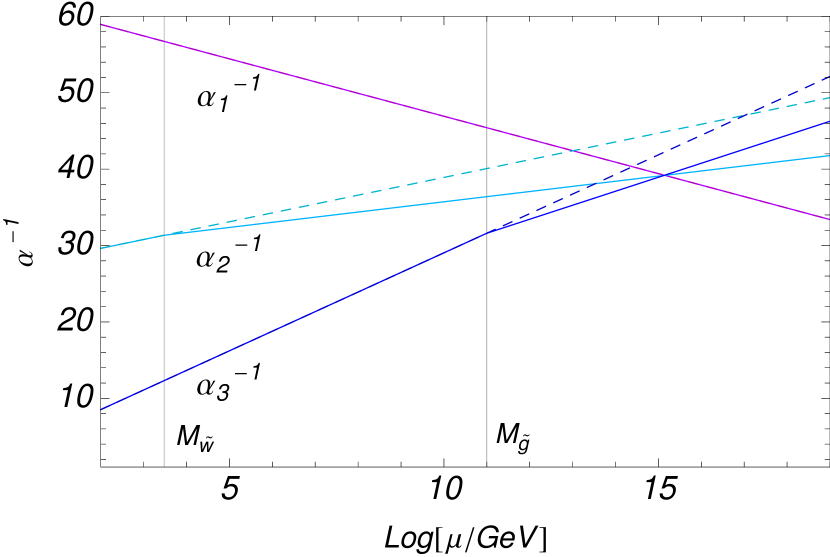
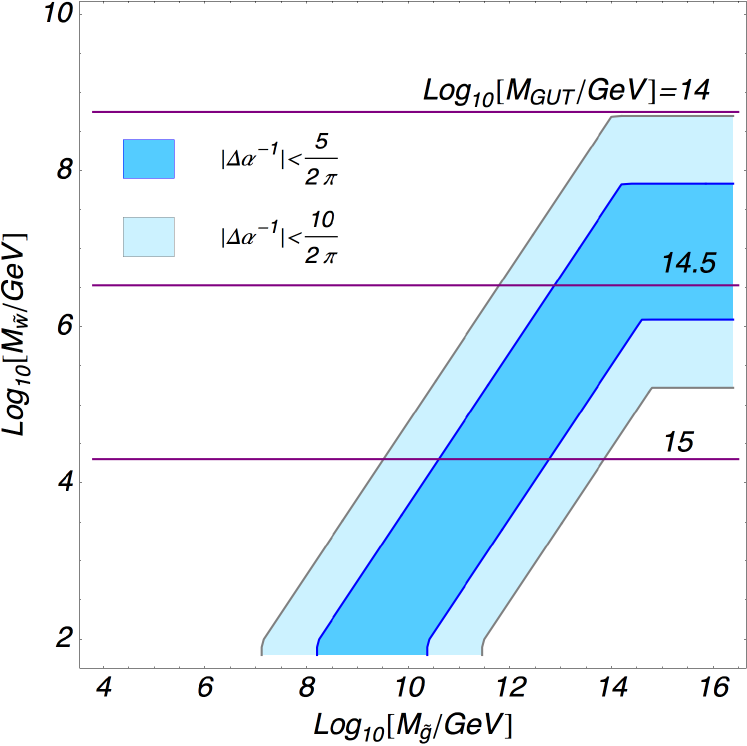
Figure 1: (Left) An example of the one-loop renormalization group evolutions of the gauge coupling constants in the extended model (solid lines). For a comparison, we show the evolutions in the SM as the dashed lines. The masses of the wino-like and gluino-like fermions are taken to be $M_{\tilde{w}}=3$ TeV and $M_{\tilde{g}}=10^{11}$ GeV, respectively. In the figures, we use $\alpha_{3}(m_{Z})^{\overline{\rm MS}}=0.1185(6)$, $N_{H}=1$. We have also taken $m_{h}=126$ GeV, and $m_{\rm top}=173.2$ GeV, although the results do not depend on these parameters significantly. (Right) The adjoint fermion masses which are preferred for a precise unification. In the (light-)blue shaded region, the three gauge coupling constants unify rather precisely, i.e. $|N_{\rm th}|<5(10)$, respectively. The horizontal lines show the contours of the $g_{1}$–$g_{2}$ unification scale.

In Ref. [11], it was found that such a precise unification is achieved by introducing only two charged particles, one is an $SU(2)_{L}$ triplet Majorana fermion and the other is an $SU(3)_{c}$ octet Majorana fermion. In this extended model, the coefficients $b_{a}$’s at the one-loop level are given by

$$b_{1}=-\left(4+\frac{N_{H}}{10}\right)\ ,\quad b_{2}=\left\{\begin{array}[]{ccc}\displaystyle{\frac{10}{3}-\frac{N_{H}}{6}}&(\mu<M_{\tilde{w}})\\ \displaystyle{2-\frac{N_{H}}{6}}&(\mu>M_{\tilde{w}})\end{array}\right.\ ,\quad b_{3}=\left\{\begin{array}[]{ccc}\displaystyle{7}&(\mu<M_{\tilde{g}})\\ \displaystyle{5}&(\mu>M_{\tilde{g}})\end{array}\right.\ ,$$ (6)

above the electroweak scale. Here, $M_{\tilde{w},\tilde{g}}$ denote the Majorana masses of the adjoint fermions. In this paper, we fix the number of the Higgs doublet $N_{H}$ to be $N_{H}=1$. In the left panel of Fig. 1, we show an example of the renormalization group evolutions of $\alpha_{a}^{-1}$ in the extended model at the one-loop level for $M_{\tilde{w}}=3$ TeV and $M_{\tilde{g}}=10^{11}$ GeV. The figure shows that the three gauge coupling constants unify rather precisely at around $10^{15}$ GeV for these adjoint fermion masses.

Now, let us discuss the mass range of the adjoint fermions which is preferred for a precise unification. For that purpose, we first need to quantify how precise the unification of the gauge coupling constants should be. One caution here is that, for a given model of the GUT, the three gauge coupling constants in the effective low energy theory are defined by matching them to the universal gauge coupling constants of the GUT by taking the threshold corrections from the charged particles with masses at the GUT scale into account. Therefore, the predictions on the adjoint fermion masses preferred by a precise unification inevitably depend on the details of the GUT models.

In this study, however, instead of specifying the GUT models, we quantify the degree of unification in terms of the size of the required threshold correction at the unification scale, so that the prediction becomes GUT model independent. Concretely, we define the unification scale $M_{\rm GUT}$ as the $g_{1}-g_{2}$ unification scale, and allows the adjoint fermion mass if the deviation of $g_{3}$ from $g_{1,2}$ at $M_{\rm GUT}$ is within some acceptance,

$$N_{\rm th}\equiv 2\pi|{\mit\Delta}\alpha^{-1}|=2\pi\times|\alpha_{\rm 1,2}^{-1}(M_{\rm GUT})-\alpha_{3}^{-1}(M_{\rm GUT})|<N_{\rm th}^{\rm(MAX)}\ .$$ (7)

Here, the quantity $N_{\rm th}$ measures how large threshold corrections are required so that the three gauge coupling constants in the low energy effective theory are obtained from a universal gauge coupling constant in the GUT. Very roughly speaking, it counts the (signed) number of charged fields in the GUT models (in the unit of the fundamental representation) which contribute to the threshold corrections at the GUT scale. For example, in the case of the MSSM, the threshold parameter satisfies $|N_{\rm th}|\mathop{}_{\textstyle\sim}^{\textstyle<}5$ [23] when the superparticles in the MSSM are at around the TeV scale. In the followings, we take $N_{\rm th}^{\rm(MAX)}=5(10)$ as the maximum acceptance so that the nominal unification in the adjoint extended model can be meaningfully interpreted as in the case of the MSSM.

In the left panel of Fig. 1, we show the degree of unification in the $M_{\tilde{g}}$–$M_{\tilde{w}}$ plane. The figures show that a precise unification, $N_{\rm th}\lesssim 5$, is achieved for $M_{\tilde{g}}\simeq 10^{7}\times M_{\tilde{w}}$. As we will discuss in section 4, the proton lifetime is predicted to be too short to be consistent with the current lower limit for $M_{\rm GUT}\lesssim 10^{15}$ GeV. Thus, by taking account of the proton lifetime, we find that a successful unification is achieved for

$$M_{\tilde{w}}\simeq 10^{2-4}\,{\rm GeV}\ ,\quad{\rm and}\quad M_{\tilde{g}}\simeq 10^{6-8}\times M_{\tilde{w}}\ ,$$ (8)

in the adjoint extension model.

3 Non-thermal Minimal Dark Matter

As we have seen in the previous section, a precise coupling unification is successfully achieved in the adjoint extension model for $M_{\tilde{w}}\simeq 10^{2-4}$ GeV. Interestingly, the wino-like fermion, i.e. the $SU(2)_{L}$ triplet Majorana fermion, has been considered as a good candidate for dark matter as the minimal dark matter model [21]. With the rather large annihilation cross section, the observed dark matter density, $\Omega h^{2}\simeq 0.1199\pm 0.0027$ [30], can be achieved by its thermal relic density for $M_{\tilde{w}}\simeq 3$ TeV [22, 21]. The predicted relic density decreases quickly for a lighter wino-like fermion.

In this section, we discuss the non-thermal production of the wino-like dark matter. The non-thermal contributions to the wino-like dark matter density have been considered in the MSSM from the late-time decays of the moduli, the gravitino, and other sectors [33, 34, 35, 17, 36, 37, 38]. When the long-lived particles decay after the wino-like fermion has freezed-out from the thermal bath, the non-thermal contributions add up to the wino-like dark matter density. With the non-thermal contributions, it is possible to explain the observed dark matter density with a wino-like fermion lighter than $3$ TeV.

Interestingly, in the adjoint extended model, we already have a candidate for the source of the non-thermal contribution, the gluino-like fermion. The gluino-like fermion is expected to be in the thermal bath if the reheating temperature after inflation is much higher than the mass of the gluino-like fermion. Such a high reheating temperature is preferred in thermal leptogenesis scenario [39]. As we will see shortly, the gluino-like fermion has an appropriate lifetime as a source of the non-thermal contribution when it decays through the higher dimensional operator suppressed by the GUT scale. Thus, in the adjoint extension model, the wino-like fermion with a mass smaller than $3$ TeV is also a viable candidate for dark matter.

3.1 Decay rate and abundance of the gluino-like fermion

In our discussion, we have implicitly assumed that there is a symmetry which makes the wino-like fermion stable so that the wino-like fermion can be a dark matter candidate. Here, we take $Z_{2}$ symmetry as an example and assume that the adjoint fermions are odd under the $Z_{2}$-symmetry while other SM particles are not charged under the symmetry. In this case, the decay of the gluino-like fermion proceeds only through higher dimensional operators such as

$${\cal L}=\frac{1}{M_{*}^{2}}({\tilde{g}}^{A}{t^{A}}{Q_{L}})^{\dagger}({\tilde{w}}^{I}{\tau^{I}}{Q_{L}})+h.c.\ ,$$ (9)

with a suppression scale $M_{*}$. Here, $Q_{L}$ denotes a doublet quark in the SM. The Gell-Mann matrices $t^{A}$ and the Pauli matrices $\tau^{I}$ are normalized so that $\mathop{\rm tr}[t^{A}t^{B}]=\delta^{AB}/2$ and $\mathop{\rm tr}[\tau^{I}\tau^{J}]=\delta^{IJ}/2$. Those decay operators can be, for example, generated by exchanges of “squark-like fields” with masses of the order of the GUT scale or above, i.e, $M_{*}\gtrsim M_{\rm GUT}$. It should be noted that this assumption is quite consistent with the adjoint extension of the SM as a low energy effective theory of the GUT in which we do not require other fields than the ones in the SM and the adjoint fermions.

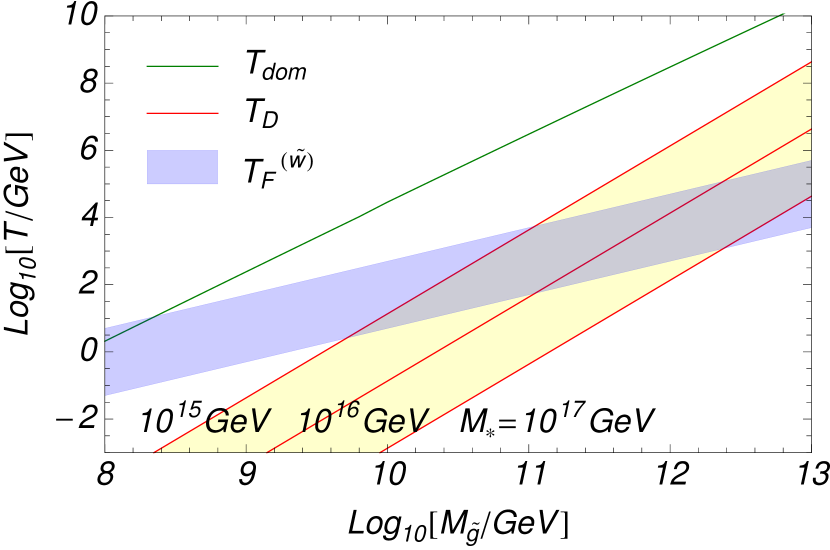
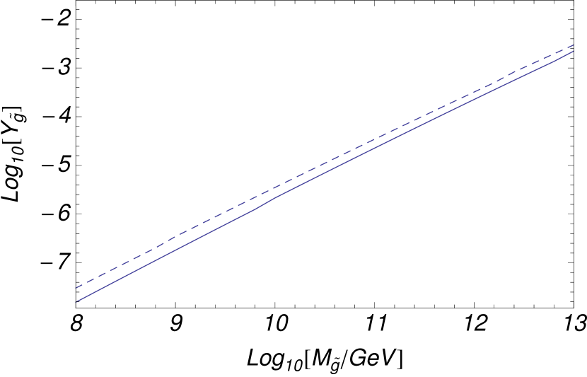
Figure 2: (Left) The decay temperature of the gluino-like fermion for a given $M_{*}$ (Eq. (12)) (red lines) and the dominate temperature (Eq. (16)) (green line). For comparison, we also show a typical freeze-out temperature of the wino-like fermion, $T_{F}(\tilde{w})\simeq M_{\tilde{w}}/20$, as a blue shaded region assuming $M_{\tilde{w}}\simeq 10^{-(6-8)}M_{\tilde{g}}$ (Eq. (8)). (Right) The yield of the gluino after freeze-out (solid line). For comparison, we show the yield without including the Sommerfeld enhancement factor as a dashed line.

Through the operator in Eq. (9), the gluino-like fermion decay into a pair of the doublet quarks and the wino-like fermion with a decay rate roughly given by

$$\Gamma_{\tilde{g}}\simeq\frac{1}{(16\pi)^{3}}\frac{M_{\tilde{g}}^{5}}{M_{*}^{4}}\ .$$ (10)

The corresponding decay temperature defined by

$$T_{D}\simeq\left(\frac{10}{\pi^{2}g_{*}}M_{\rm PL}^{2}\Gamma_{\tilde{g}}^{2}\right)^{1/4}\ ,$$ (11)

is estimated to be,

$$T_{D}\simeq 44\,{\rm GeV}\times\left(\frac{111}{g_{*}}\right)^{1/4}\left(\frac{M_{\tilde{g}}}{10^{11}\,{\rm GeV}}\right)^{5/2}\left(\frac{10^{16}\,\rm GeV}{M_{*}}\right)^{2}\ .$$ (12)

Here, $M_{\rm PL}\simeq 2.44\times 10^{18}$ GeV is the reduced Planck scale and we have fixed the effective number of the massless degrees of freedom to be $g_{*}\simeq 111$ which includes the SM particles and the wino-like fermions.

In the left panel of Fig. 2, we show the decay temperature of the gluino-like fermion for given values of $M_{*}$. For comparison, we also show a typical freeze-out temperature of the wino-like fermion, $T_{F}^{(\tilde{w})}\simeq M_{\tilde{w}}/25$, as a blue shaded region assuming $M_{\tilde{w}}\simeq 10^{-(6-8)}M_{\tilde{g}}$. As a result, the decay temperature is expected to be below the freeze-out temperature for $M_{*}\gtrsim M_{\rm GUT}\simeq 10^{15}$ GeV, and hence, the gluino-like fermion in the intermediate scale can be a non-thermal source of the wino-like fermion.

Let us estimate the number density of the gluino-like fermion before its decay. When the reheating temperature of the universe after inflation is much higher than the mass of the gluino-like fermion, the gluino-like fermion is in the thermal bath. The gluino-like fermion eventually decouples from the thermal bath when the cosmic temperature decreases below the freeze-out temperature, $T_{F}^{(\tilde{g})}$ which is given iteratively by

$$\ln\left[\frac{\left\langle{\sigma_{\tilde{g}}v}\right\rangle}{\pi^{3}}\sqrt{\frac{45\pi}{g_{*}(T_{F})}}M_{\rm PL}M_{\tilde{g}}g_{\tilde{g}}x_{F}^{1/2}\right]=x_{F}\ ,$$ (13)

where $x\equiv M_{\tilde{g}}/T$ and $g_{\tilde{g}}=2\times 8$ [41]. Here, $\left\langle{\sigma_{\tilde{g}}v}\right\rangle$ denotes the thermally averaged cross section of the gluino-like fermion. The resultant relic density of the gluino-like fermion per the entropy density $s$ is then given by,

$$Y_{\tilde{g}}\simeq\sqrt{\frac{45}{\pi}}\left(\int_{x_{F}}^{\infty}\frac{h_{*}(T)}{\sqrt{g_{*}(T)}}\frac{M_{\rm PL}M_{\tilde{g}}}{x^{2}}\left\langle{\sigma_{\tilde{g}}v}\right\rangle dx\right)^{-1}\simeq K^{-1}\times\sqrt{\frac{45}{g_{*}(T_{F})\pi}}\frac{x_{F}}{\alpha_{3}^{2}}\frac{M_{\tilde{g}}}{M_{\rm PL}}\ .$$ (14)

Here, $h_{*}(T)$ is the entropy degree-of-freedom counting factor, which is very close to $g_{*}(T)$. In the right panel of Fig. 2, we show the yield of the gluino-like fermion after freeze-out. In our analysis, we have used the annihilation cross section given in Ref. [42] where the Sommerfeld enhancement factors are taken into account (see also Ref. [43]). The final expression of Eq. (14) fairly reproduces our numerical result in Fig. 2 for a numerical factor $K\simeq 10$.

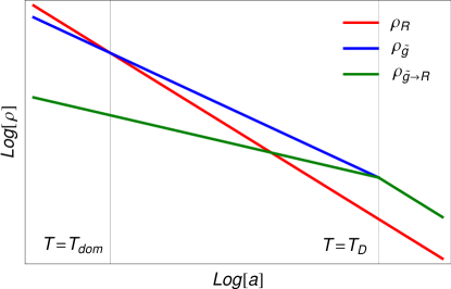
Figure 3: The evolution of the energy densities of the radiation and the gluino-like fermion. Here, the energy density of the original radiation (red line) scales as $a^{-4}$ while the one of the gluino-like fermion scales as $a^{-3}$ (blue line). The radiation energy released by the occasional decay of the gluino-like fermion scales as $a^{-3/2}$ (green line).

As the cosmic temperature further decreases, the energy density of the gluino-like fermion becomes comparable to the radiation energy,

$$\rho_{\rm tot}=\rho_{R}+M_{\tilde{g}}Y_{\tilde{g}}s\ ,$$ (15)

and eventually dominates the energy density when the temperature becomes below $T_{\rm dom}$;

$$T_{\rm dom} \simeq \frac{4}{3}M_{\tilde{g}}Y_{\tilde{g}}\simeq\frac{4}{3K}\times\sqrt{\frac{\pi}{45g_{*}(T_{F})}}\frac{x_{F}}{\alpha_{3}^{2}}\frac{M_{\tilde{g}}^{2}}{M_{\rm PL}}$$ (16)

$$\simeq {3\times 10^{6}}\,{\rm GeV}\left(\frac{M_{\tilde{g}}}{10^{11}\,\rm GeV}\right)^{2}.$$ (17)

By comparing with Eq. (12), the domination temperature is higher than $T_{D}$ and $T_{F}^{({\tilde{w}})}$ in most parameter space, and hence, the gluino-like fermion decays after it dominates the energy density of the universe (see the green-line in the left panel of Fig. 2).

In Fig. 3, we show a schematic picture of the evolutions of the energy densities of the radiation and the gluino-like fermion after the freeze-out of the gluino-like fermion. Once the domination by the gluino-like fermion happens, the energy density of the original radiation decreases and its temperature scales as $a^{-1}$ (the red line in the figure) with $a$ being the scale factor of the universe. At the same time, the gluino-like fermion gradually releases its energy into radiation where the released radiation energy density scales as $a^{-3/2}$ (the green line in the figure). Then, at around the decay temperature $T_{D}$, the most gluino-like fermion decays into radiation, after that its energy density decreases exponentially. It should be noted that the scale factors at the domination time and the decay time are related to the domination temperature and the decay temperature via,

$$\left(\frac{a_{\rm dom}}{a_{D}}\right)^{3}\simeq\left(\frac{H_{D}}{H_{\rm dom}}\right)^{2}\simeq\left(\frac{T_{D}}{T_{\rm dom}}\right)^{4}\ ,$$ (18)

where $H_{D}$ and $H_{\rm dom}$ denote the Hubble parameter at $T_{D}$ and $T_{\rm dom}$, respectively. Thus, the radiation energy density is dominated by the one from the gluino-decay for

$$T\lesssim T_{*}\equiv T_{D}\times\left(\frac{T_{\rm dom}}{T_{D}}\right)^{1/5}\ ,$$ (19)

although the final relic density of the wino-like fermion does not depend on the detailed evolution of the thermal bath before $T_{D}$.

3.2 Non-thermal contribution to the relic density of the wino-like fermion

Now, let us discuss how the wino-like fermion is produced by the decay of the gluino-like fermion. As we have discussed above, the gluino-like fermion decays through the higher dimensional operator which produces a wino-like fermion and a pair of quarks whose initial energies are of ${\cal O}(M_{\tilde{g}})$. The high energetic quarks are immediately resolved into the thermal-bath and reach to the chemical equilibrium, which gradually heats up the radiation (see the appendix A). The produced charged components of the wino-like fermion also lose their energies immediately via the electromagnetic interactions with the thermal-bath [40]. The neutral components of the wino-like fermion are on the other hand excited to the charged winos via inelastic scattering and they lose energies as the charged components.

It should be noted that the wino-like fermions are also produced by high energy injection of the quarks into the thermal bath [45]. The production cross section of the wino-like fermion via interactions between the injected quarks and the quarks in the thermal-bath are roughly given by,

$$\sigma_{\tilde{w}}\simeq\frac{\alpha_{2}\alpha_{3}}{ET}\ .$$ (20)

Here, $E$ is the energy of the quarks/gluons which are induced during the thermalization process of the injected quarks from the decay of the gluino-like fermion. The number of those energetic particles per a decay of the gluino-like fermion is given by,

$$N(E)\sim\frac{M_{\tilde{g}}}{E}\ .$$ (21)

The energy loss rate of the quarks/gluons with energy $E$ via inelastic soft scattering by the QED interaction is, for example, given by [46] (see also [47]),

$$\Gamma_{\rm split}(E)\sim\alpha_{3}^{2}T\sqrt{\frac{T}{E}}\ .$$ (22)

Thus, the probability of the pair production of the wino-like fermion from each particle with an energy $E$ is given by,

$$P_{\tilde{w}}={\min}\left[1,\sigma_{\tilde{w}}T^{3}\Gamma_{\rm split}^{-1}\right]\sim{\min}\left[1,\frac{\alpha_{2}}{\alpha_{3}}\sqrt{\frac{T}{E}}\right]\ .$$ (23)

This probability is maximized for $E=E_{\rm th}\sim M_{\tilde{w}}^{2}/T$ for $T\ll M_{\rm w}$. As a result, for $T\ll M_{\tilde{w}}$, the number of the wino-like fermion produced by a decay of the gluino-like fermion is given by,

$$N_{\tilde{w}}={\max}\left[1,N(E_{\rm th})\times P_{\tilde{w}}\right]\ .$$ (24)

In our model, we find that $N_{\tilde{w}}\gg 1$ in most parameter space for $T_{D}\gtrsim 1$ GeV, and hence, the wino-like fermion produced by the gluino-decay is dominated by the contribution from the secondary generation. As we will see, the final relic abundance of the wino-like fermion, however, does not depend on $N_{\tilde{w}}$ significantly as long as $N_{\tilde{w}}\gtrsim 1$ and the final abundance is mainly determined by the annihilation rate of the wino-like fermion at the time of $T\simeq T_{D}$.

3.3 Relic density of the wino-like fermion

Let us estimate the relic density of the wino-like fermion by solving the set of the Boltzmann equations,

$$\frac{dn_{\tilde{w}}}{dt}+3Hn_{\tilde{w}} = -\left\langle{\sigma_{\mathrm{eff}}v}\right\rangle(n^{2}_{\tilde{w}}-n^{2}_{\tilde{w},\mathrm{eq}})+N_{\tilde{w}}\Gamma_{\tilde{g}}n_{\tilde{g}}\ ,$$ (25)

$$\frac{dn_{\tilde{g}}}{dt}+3Hn_{\tilde{g}} = -\Gamma_{\tilde{g}}n_{\tilde{g}}\ ,$$ (26)

$$\frac{d\rho_{\mathrm{R}}}{dt}+4H\rho_{\mathrm{R}} = (M_{\tilde{g}}-N_{\tilde{w}}M_{\tilde{w}})\Gamma_{\tilde{g}}n_{\tilde{g}}+M_{\tilde{w}}\left\langle{\sigma_{\mathrm{eff}}v}\right\rangle n^{2}_{\tilde{w}}\ .$$ (27)

Here, $n_{\tilde{w}}$ and $n_{\tilde{g}}$ are the number densities of wino-like fermions and gluino-like fermions, respectively, $n_{\tilde{w},\rm eq}$ the thermal-equilibrium value of $n_{\tilde{w}}$ [36]. In Eq. (27), the heat injection from the wino-like fermions is proportional to $M_{\tilde{w}}$, since the wino-like fermions loose their energy into the thermal bath immediately after the production. Accordingly, the Hubble parameter $H$ during the non-thermal production period is approximated by,

$$H^{2}=\frac{1}{3M_{\rm PL}^{2}}\left(M_{\tilde{g}}n_{\tilde{g}}+\rho_{R}\right)\ ,$$ (28)

which is eventually dominated by the contributions from the radiation energy for $T\lesssim T_{D}$. It should be noted that the thermally averaged effective annihilation cross section, $\left\langle{\sigma_{\mathrm{eff}}v}\right\rangle$, is affected by the coannihilation process and the Sommerfeld enhancement, which significantly enhances the cross section compared with the one predicted by tree-level contributions in the case of wino-like $SU(2)_{L}$ adjoint fermion [22]. In our numerical calculation, we have taken into account those enhancement factors according to [22, 36].

In order to obtain an approximated relic abundance, let us first consider the situation where all gluino-like fermions decay into wino-like fermion instantaneously at $T_{\mathrm{eff}}\simeq T_{D}$. In this case, Eq. (25) is reduced to

$$\frac{dn_{\tilde{w}}}{dt}+3Hn_{\tilde{w}} = -\left\langle{\sigma_{\mathrm{eff}}v}\right\rangle n^{2}_{\tilde{w}}\ ,$$ (29)

for $T\ll T_{\rm eff}$ with $H$ dominated by the radiation contribution. The solution of this reduced equation is given by,

$$\left.\frac{1}{Y_{\tilde{w}}}\right|_{T\rightarrow 0}=\frac{1}{Y_{\tilde{w}}^{\rm(init)}}+\int_{0}^{T_{\mathrm{eff}}}\frac{\left\langle{\sigma_{\mathrm{eff}}v}\right\rangle s}{HT}dT\ ,$$ (30)

where $Y_{\tilde{w}}^{\rm(init)}$ accounts for the non-thermal production by the decay of the gluino-like fermions at $T_{\rm eff}$, i.e.

$$Y_{\tilde{w}}^{\rm(init)}\simeq\left.\frac{N_{\tilde{w}}n_{\tilde{g}}}{s}\right|_{T\simeq T_{\rm eff}}\simeq N_{\tilde{w}}\frac{3T_{\rm eff}}{4M_{\tilde{g}}}\ ,$$ (31)

where we have neglected thermally produced component and assumed that $T_{\rm eff}<T_{F}^{(\tilde{w})}$. By remembering that $N_{\tilde{w}}\gg 1$, we find that $Y_{\tilde{w}}^{\rm(init)}$ is much larger than the inverse of the second term of Eq. (30),

$$Y_{\tilde{w}}^{\rm(asym)}\simeq\left(\int_{0}^{T_{\mathrm{eff}}}\frac{\left\langle{\sigma_{\mathrm{eff}}v}\right\rangle s}{HT}dT\right)^{-1}\ ,$$ (32)

which can be further reduced

$$\bar{Y}_{\tilde{w}}^{\rm(asym)}\simeq\left.\frac{H}{\left\langle{\sigma_{\mathrm{eff}}v}\right\rangle s}\right|_{T\simeq T_{\mathrm{eff}}}\ .$$ (33)

when $\left\langle{\sigma_{\mathrm{eff}}v}\right\rangle$ does not depend on temperature.

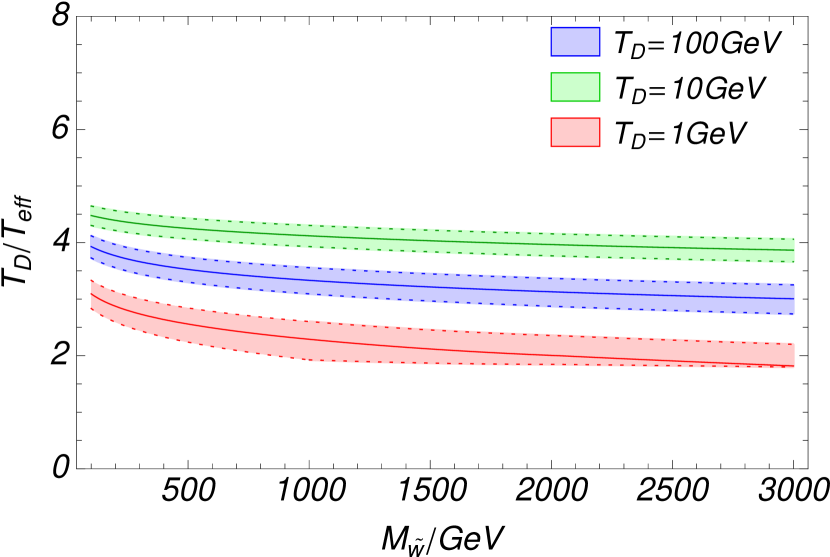
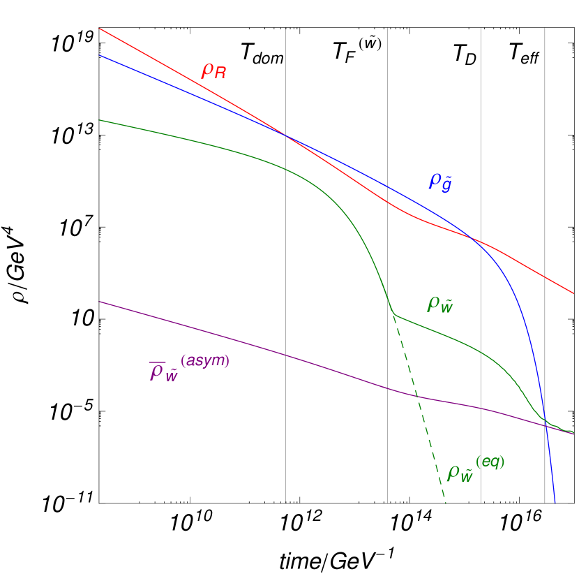
Figure 4: (Left) The ratio between $T_{D}$ and the effective temperature of the non-thermal production $T_{\rm eff}$ for given $T_{D}$. The solid lines show the ratios for $P_{\tilde{w}}$ given in Eq. (23). For comparisons, the ratios for ten times smaller (larger) values of $P_{\tilde{w}}$ than the one given in Eq. (23) are shown as the lower (upper) dotted lines. (Right) The evolutions of the energy densities for $M_{\tilde{w}}=1$ TeV, $M_{\tilde{g}}=10^{10}$ GeV, and $M_{*}=10^{15}$ GeV obtained by solving the Boltzmann equations numerically.

In reality, the non-thermal production is not an immediate process. However, by appropriately relating the effective temperature $T_{\rm eff}$ to the decay temperature $T_{D}$, we can obtain a good approximation of the yield of the wino-like fermion by using the above simplified solution in Eq. (32). To find the relation between $T_{D}$ and $T_{\rm eff}$, let us look at the Boltzmann Eq. (26) at the temperature just below $T_{D}$;

$$\frac{dn_{\tilde{w}}}{dt}+3Hn_{\tilde{w}} = -\left\langle{\sigma_{\mathrm{eff}}v}\right\rangle n^{2}_{\tilde{w}}+N_{\tilde{w}}\Gamma_{\tilde{g}}\frac{\rho_{\tilde{g}}}{M_{\tilde{g}}}e^{-\Gamma_{\tilde{g}}t}\ .$$ (34)

By assuming the radiation domination at that period, this equation can be rewritten in terms of the temperature,

$$HT\frac{dY_{\tilde{w}}}{dT}=\left\langle{\sigma_{\mathrm{eff}}v}\right\rangle sY^{2}_{\tilde{w}}-N_{\tilde{w}}\Gamma_{\tilde{g}}\frac{3T}{4M_{\tilde{g}}}e^{-\frac{3}{2}\left(\frac{T_{D}}{T}\right)^{2}}.$$ (35)

Since $T_{\mathrm{eff}}$ can be regarded as the temperature at which the source term is dumped and becomes comparable to the first term, we find the relation between $T_{\rm eff}$ and $T_{D}$ by,

$$T_{\mathrm{eff}}\simeq\sqrt{\frac{3}{2}}\,T_{D}\times\left[\log\left[{\frac{3N_{\tilde{w}}Y_{0}}{\bar{Y}_{\tilde{w}}^{\rm(asym)}}}\right]\right]^{-\frac{1}{2}},$$ (36)

where $Y_{0}=3T/4M_{\tilde{g}}$, and we have used $\Gamma_{\tilde{g}}\simeq 3H$ at $T\simeq T_{D}$.

In the left panel of Fig. 4, we show the relation between $T_{D}$ and $T_{\rm eff}$ as a function of $M_{\tilde{w}}$ for given values of $T_{D}$. In the figure, the solid lines show the ratios for $P_{\tilde{w}}$ given in Eq. (23). For comparisons, we also show the ratios for ten times smaller (larger) values of $P_{\tilde{w}}$ than the one given in Eq. (23) as the dotted lines. The figure shows that the ratios do not depend on the values of $P_{\tilde{w}}$ significantly. It should be also noted that we have taken $M_{\tilde{g}}=10^{7}\times M_{\tilde{w}}$ in the figure, although $M_{\tilde{g}}$ dependence is not significant since $N_{\tilde{w}}$ is proportional to $M_{\tilde{w}}$ while $Y_{0}$ is inversely proportional to $M_{\tilde{g}}$ in most parameter region. In the right panel of Fig. 4, we also show an example of the evolutions of the energy densities obtained by the Boltzmann equation numerically. The figure shows that the energy density is dominated by gluino-like fermions at $T_{\rm dom}$. After that the wino-like fermions decouple from the thermal bath at around $T^{(\tilde{w})}_{F}\simeq m_{\tilde{w}}/25$. At the decay temperature $T_{D}$, the gluino-like fermion decays and the energy density gets dominated by the radiation energy. Finally, the energy density of the wino-like fermion approaches to its asymptotic value,

$$\rho^{\rm(asym)}_{\tilde{w}}=M_{\tilde{w}}Y_{\tilde{w}}^{\rm(asym)}\times s(T)\ .$$ (37)

The figure shows that the asymptotic solution in Eq. (32) gives a fairly good approximation.

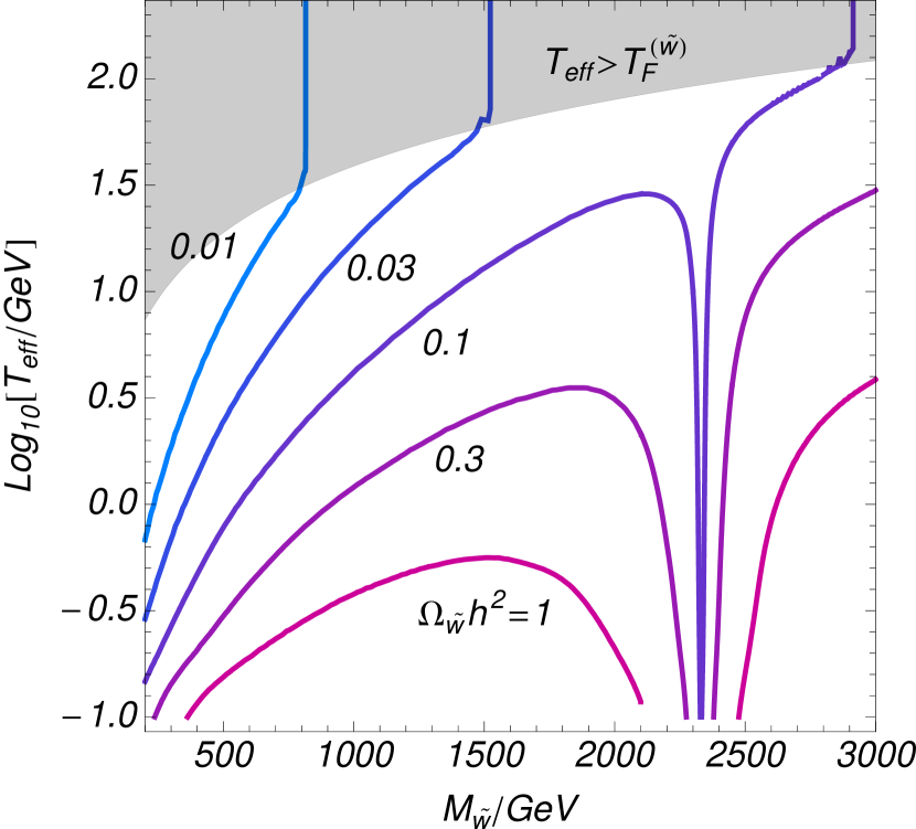
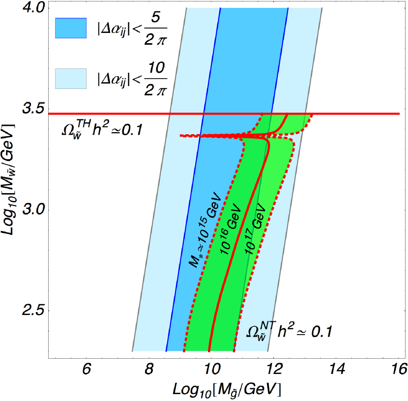
Figure 5: (Left) Contour plots of $\Omega_{\tilde{w}}h^{2}$ on the $T_{\rm eff}$-$M_{\tilde{w}}$ plane. (Right) Contour plots of $M_{*}$ which provides an appropriate decay temperature of the gluino-like fermion for $\Omega_{\tilde{w}}h^{2}\simeq 0.1146$ via the non-thermal production. Here, we put the superscripts $\Omega_{\tilde{w}}^{TH}h^{2}\simeq 0.1$ (thermal) and $\Omega_{\tilde{w}}^{NT}h^{2}\simeq 0.1$ (non-thermal) to indicate the main contributions to the dark matter abundance. The precise unification conditions in Fig. 1 are also shown.

In the left panel of Fig. 5, we show the contours of $\Omega_{\tilde{w}}h^{2}$ in the $T_{\rm eff}-M_{\tilde{w}}$ plane. For a given mass of the wino-like fermion, the relic abundance becomes insensitive to $T_{\rm eff}$ when $T_{\rm eff}$ is so high that the wino-like fermion is still in thermal equilibrium after $T_{\mathrm{eff}}$. In such region, the relic abundance is dominated by thermal relic. The abundance of the wino-like fermion is significantly suppressed at around $M_{\tilde{w}}\sim 2300~{}\mathrm{GeV}$ where the annihilation cross section of the wino-like fermion is significantly enhanced by the Sommerfeld enhancement. We see from the left panel of Fig. 5 that the region with a wino-like fermion mass smaller than $3$ TeV can be consistent with the observed dark matter abundance for $T_{\rm eff}={\cal O}(1$–$10)$ GeV.

From Eqs. (12) and (36), we can estimate the required size of $M_{*}$ to achieve an appropriate decay temperature for $\Omega_{\tilde{w}}h^{2}\simeq 0.1$ as a function of $M_{\tilde{w}}$ and $M_{\tilde{g}}$. In the left panel of Fig. 5, we show the contour plot of the required $M_{*}$ by overlaying the left panel of Fig. 1. The figure shows that in the mass region which leads to the appropriate decay temperature for $M_{*}\simeq 10^{15-17}$ GeV is consistent with the successful unification. Therefore, we find that gluino-like fermion can be a successful source of the non-thermal wino-like fermion without requiring lighter fields than the GUT scale.

4 Constraints from Proton Decay

In section 2, we discussed the mass range of the adjoint fermions which leads to a precise unification of the three gauge coupling constants. There, we found that the GUT scale (defined as a $g_{1}-g_{2}$ unification scale) has a strong correlation with the mass of the wino-like fermion. The GUT scale is, in turn, correlated with the mass of the massive gauge bosons in the GUT (i.e. the GUT gauge boson), which causes a decay of the proton [2, 4]. In this section, we discuss the proton lifetime expected in the adjoint extension model.

To estimate the mass of the GUT gauge bosons, let us review the matching conditions of the three gauge coupling constants to the universal gauge coupling constant of the GUT at the one-loop level;

$$\frac{1}{\alpha_{3}(\mu)} = \frac{1}{\alpha_{\rm GUT}(\Lambda)}+\frac{1}{2\pi}\left(\beta_{3}^{(L)}\log\frac{\mu}{\Lambda}+\beta_{3}^{(XY)}\log\frac{M_{V}}{\Lambda}+{\mit\Delta}\beta_{3}\log\frac{{\cal M}_{3}}{\Lambda}\right)\ ,$$

$$\frac{1}{\alpha_{2}(\mu)} = \frac{1}{\alpha_{\rm GUT}(\Lambda)}+\frac{1}{2\pi}\left(\beta_{2}^{(L)}\log\frac{\mu}{\Lambda}+\beta_{2}^{(XY)}\log\frac{M_{V}}{\Lambda}+{\mit\Delta}\beta_{2}\log\frac{{\cal M}_{2}}{\Lambda}\right)\ ,$$

$$\frac{1}{\alpha_{1}(\mu)} = \frac{1}{\alpha_{\rm GUT}(\Lambda)}+\frac{1}{2\pi}\left(\beta_{1}^{(L)}\log\frac{\mu}{\Lambda}+\beta_{1}^{(XY)}\log\frac{M_{V}}{\Lambda}+{\mit\Delta}\beta_{1}\log\frac{{\cal M}_{1}}{\Lambda}\right)\ .$$ (38)

Here, $M_{V}$ denotes the mass of the GUT gauge boson, $\mu$ the renormalisation scale, and $\Lambda$ the scale at which the boundary condition of $\alpha_{\rm GUT}$ is given. The coefficients of the beta function are given by

$$\beta_{3}^{(L)} = 5\ ,\quad\beta_{2}^{(L)}=\frac{11}{6}\ ,\quad\beta_{1}^{(L)}=-\frac{41}{10}\ ,$$

$$\beta_{3}^{(XY)} = 7\ ,\quad\beta_{2}^{(XY)}=\frac{21}{2}\ ,\quad\beta_{1}^{(XY)}=-\frac{25}{2}\ ,$$ (39)

respectively. The final terms in each matching condition collectively denote the contributions from other multiplets at the GUT scale than the ones in the SM, the adjoint fermions, and the GUT gauge bosons, which depend on the details of the GUT models.

Thinking along the same lines in section 2, let us give an model independent estimation on $M_{V}$ in the following way. First, we take $\mu=\Lambda=M_{\rm GUT}$ without loss of generality. Then, let us define

$${\mit\Delta}\alpha^{-1}_{ij}\equiv\frac{1}{2\pi}\left(\beta_{i}^{(XY)}-\beta_{j}^{(XY)}\right)\log\frac{M_{V}}{M_{\rm GUT}}\ ,$$ (40)

which encodes how large GUT breaking threshold effects are required to match the three gauge coupling constants to the universal one at $\mu=M_{\rm GUT}$. If ${\mit\Delta}\alpha^{-1}_{ij}$’s are too large, the nominal coupling unification in the adjoint extension of the SM is just an accidental one achieved by accidental cancellations between large GUT breaking contributions. Thus, as in the track of the discussion in section 2, we require that ${\mit\Delta}\alpha^{-1}_{ij}$’s are not too large. Concretely, we adopt the same criteria in Eq. (7), i.e.

$$|{\mit\Delta}\alpha_{13}|<\frac{N_{\rm th}^{\rm(MAX)}}{2\pi}\ .$$ (41)

Altogether, by substituting the $\beta$’s in Eq. (4), this requirement amounts to a constraint on the GUT gauge boson mass,

$$M_{V}=M_{\rm GUT}\times\exp\left[{\pm\left|\frac{N_{\rm th}^{\rm(MAX)}}{\beta_{2}^{(XY)}-\beta_{1}^{(XY)}}\right|}\right]=M_{\rm GUT}\times\exp\left[{\pm\left|\frac{2N_{\rm th}^{\rm(MAX)}}{35}\right|}\right]\ ,$$ (42)

where we again take $N_{\rm th}^{\rm(MAX)}$ to be $5$ or $10$ as reference values. In the left panel of Fig. 6, we show the mass range of $M_{V}$ as a function of $M_{\tilde{w}}$. The figure shows that $M_{V}={\cal O}(10^{15})$ GeV in the whole mass range of the wino-like fermion.

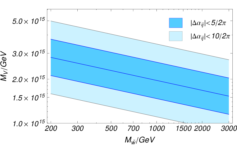
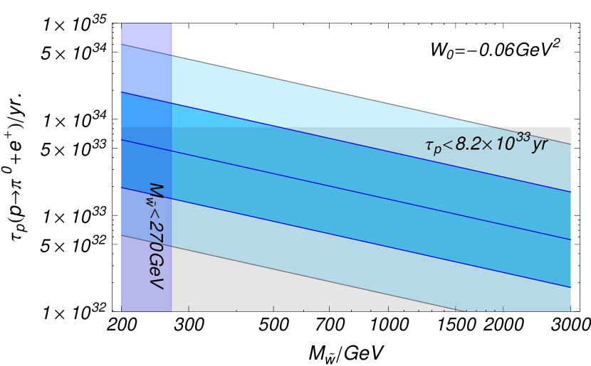
Figure 6: (Left) The mass range of the GUT gauge boson as a function of the mass of the wino-like fermion. We have assumed $N_{\rm th}^{\rm(MAX)}=5$ for blue (dark) shaded region and $N_{\rm th}^{\rm(MAX)}=10$ for light-blue (light) shaded region in Eq. (42). (Right) The proton lifetime via $p\to\pi^{0}+e^{+}$ assuming the GUT gauge boson mass in Eq. (42). Here, we have fixed the form factor to be $W_{0}=-0.06$ GeV² so that the exclusion limit is conservative. The horizontally shaded region is excluded by the current lower limit $\tau_{p}\gtrsim 8.2\times 10^{33}$yr. The vertically shaded region is excluded by the lower limit, $M_{\tilde{w}}\gtrsim 270$ GeV.

The proton decay process, $p\to\pi^{0}+e^{+}$, proceeds through effective operators,

$${\cal L}=\frac{g_{\rm GUT}^{2}}{M_{V}^{2}}\left[A_{R}\,(\bar{d}_{R}^{\dagger}\bar{u}_{R}^{\dagger})(u_{L}e_{L})+A_{L}(1+|V_{ud}|^{2})\,(u_{L}d_{L})(\bar{u}_{R}^{\dagger}\bar{e}_{R}^{\dagger})+h.c.\right]\ ,$$ (43)

(see for example Ref. [48]). Here, $V_{ud}\simeq 0.974$ denotes the $ud$-component of the Cabibbo-Kobayashi-Masukawa matrix. The coefficients $A_{R,L}$ represent the renormalization factors of the above operators between the GUT scale to a lower energy scale. At the renormalization scale $\mu=2$ GeV, the coefficients $A_{R,L}$ are given by,

$$A_{R,L}=A_{R,L}^{\rm SM}\times\left(\frac{\alpha_{2}(M_{\tilde{w}})}{\alpha_{\rm GUT}}\right)^{\frac{9}{4}\left(b_{2}^{-1}(\mu>M_{\tilde{w}})-b_{2}^{-1}(\mu<M_{\tilde{w}})\right)}\times\left(\frac{\alpha_{3}(M_{\tilde{g}})}{\alpha_{\rm GUT}}\right)^{2\left(b_{3}^{-1}(\mu>M_{\tilde{g}})-b_{3}^{-1}(\mu<M_{\tilde{g}})\right)}\ .$$ (44)

Here, $A_{R,L}^{\rm SM}$ is the renormalization factor without having the adjoint fermions below the GUT scale which have been estimated to be $A_{R}^{\rm SM}\simeq 3$ and $A_{L}^{\rm SM}\simeq 3.2$ at $\mu=2$ GeV [48]. We find that $A_{R,L}$ is not very different from $A_{R,L}^{\rm SM}$, $A_{R,L}/A_{R,L}^{\rm SM}\simeq 1.0$–$1.2$, for wide ranges of $M_{\tilde{w}}$ and $M_{\tilde{g}}$.

Altogether, the resultant lifetime of the proton is given by,

$$\tau(p\to\pi^{0}+e^{+})\simeq 4.8\times 10^{33}\,{\rm yr}\times\left(\frac{A_{L,R}^{\rm SM}}{A_{L,R}}\right)^{2}\left(\frac{1/40}{\alpha_{G}}\right)^{2}\left(\frac{M_{V}}{10^{15.5}\,\rm GeV}\right)^{4}\left(\frac{0.103\,{\rm GeV}^{2}}{|W_{0}|}\right)^{2}\ ,$$ (45)

where $W_{0}$ denotes the form factor of the proton decay operators between the proton and the pion states. In this analysis, we use $W_{0}\simeq-0.103$ GeV² which is obtained by lattice QCD simulations [49] with a total error about $30$–$40$%. In the right panel of Fig. 6, we show the predicted proton lifetime assuming the GUT gauge boson mass ranges in Eq. (42). We also show the lower limit on the proton lifetime at 90% confidence level by the Super-Kamiokande with the total exposure $140$ kton-yrs. $\tau_{p}>8.2\times 10^{33}$ yr. [50]. The figure shows that $M_{\tilde{W}}\gtrsim 550$ GeV ($1.9$ TeV) has been excluded due to a too short proton lifetime for $N_{\rm th}^{\rm(MAX)}=5\,(10)$. The figure also shows that the whole mass range of the wino-like fermion can be surveyed by the Hyper-Kamiokande experiment which is sensitive to the proton lifetime of $O(10^{35})$ yr [51].

Before closing our discussion, let us summarize other constraints on the wino-like fermions. Due to the small mass difference between the charged and the neutral components of the wino-like fermion, the charged wino-like fermion has a rather long lifetime, and hence, it leaves a disappearing track once it is produced at the collider experiments. By searching for the disappearing charged tracks, the ATLAS collaboration has put a stringent constraints on the mass of the wino-like fermion mass,

$$M_{\tilde{w}}\gtrsim 270\,{\rm GeV}\ ,$$ (46)

with $20$ fb^-1 data at 8 TeV running [52]. At the 14 TeV running, the limit is expected to be pushed up to $500$ GeV with $100$ fb^-1 data [53]. For more details on the future prospects of the searches for the wino-like fermion at the collider experiments, see Ref. [54].

The mass of the wino-like fermion is also constrained from the indirect detection of dark matter using cosmic-rays. Currently, the most robust limit comes from the continuum gamma-ray searches from dwarf spheroidal galaxies at the Fermi-LAT experiment which has excluded $M_{\tilde{w}}\lesssim 320$ GeV and $2.25$ TeV$\lesssim M_{\tilde{w}}\lesssim 2.43$ TeV at the 95% confidence level using four-year data [55]. The searches for monochromatic gamma-rays from the galactic center [58] as well as the dwarf spheroidal galaxies [59] by the H.E.S.S experiments also put constraints on the wino-like fermion mass. Those constraints are, however, less stringent compared with the above constraints due to large uncertainties of the dark matter profile at the galaxy center (see e.g. Ref. [60]) and the small cross section into the monochromatic gamma-rays. For the constraints from other cosmic-rays, see e.g. Ref. [63].

The direct detection experiments of the wino-like fermion are, on the other hand, challenging for on-going experiments since it has no tree-level $\tilde{w}-\tilde{w}-$Higgs nor $\tilde{w}-\tilde{w}-Z$ interactions. As estimated in [69], however, loop suppressed interactions lead to a spin-independent nucleon cross section of $\sigma_{\tilde{w}N}={\cal O}(10^{-47})\,{\rm cm}^{2}$, with which it might be possible to test the model by such as the LZ experiment [70] and the DARWIN experiment [71] for $M_{\tilde{w}}\lesssim 1$ TeV.

5 Conclusions

In this paper, we revisited a small extension of the SM which achieve a precise coupling unification while providing a good dark matter candidate, the wino-like fermion. As we have discussed, the non-thermal production of the wino-like fermion from the gluino-like fermion can dominate over the thermal contribution which allows the lighter wino-like dark matter than the minimal dark matter scenario. With such a lighter wino-like dark matter, the proton lifetime is predicted above the current lower limit by the Super Kamiokande experiment. We also found that the most parameter space can be tested through the combination of the direct searches at the LHC experiments, the cosmic gamma-ray searches and the search for the proton decay at the Hyper-Kamiokande experiment.

As a final remark, let us comment on the possible warm component of the wino-like dark matter. As we have discussed in section 3, most of the wino-like dark matter produced by the decay of the gluino-like fermion immediately blends into the thermal bath. However, if the neutral wino-like fermion is produced with a very small momentum for $T_{\rm eff}={\cal O}(100)$ MeV it cannot lose its momentum very efficiently, which may end up with a warm component. Thus, a very small fraction of the wino-like dark matter can be a warm component of dark matter, which might leave some imprints on the small scale structure [40].

Appendix A Fate of the high energetic quarks

In this appendix, let us discuss how the produced quarks by the decay of the gluino-like fermion form the thermal bath. When the universe is dominated by radiation, the high energy quarks emitted by the decay of the gluino-like fermion lose their energy very quickly and is resolved into radiation immediately. Even after the gluino-like fermion dominates the universe, the radiation energy is dominated by the original radiation for $T>T_{*}$ in Eq. (19). Thus, the produced quark is again resolved into the radiation quickly for $T>T_{*}$.

Once the temperature becomes lower than $T_{*}$, on the other hand, the radiation energy is dominated by the one from the decay of the gluino-like fermion. Since each quark has much higher energy than the temperature, the number density of the quarks are much smaller than the one of the radiation in the thermal equilibrium. Thus, in this period, there should be efficient inelastic interactions which change the number of the particles so that the produced quarks form the thermal radiation.

In our scenario, the thermal bath exists before the decay of the gluino-like fermion, and hence, the thermalization proceeds via inelastic interactions between the injected quarks and the pre-existing thermal bath. The energy loss rate in the thermalization process is given by [46] (see also [47]),

$$\frac{dE}{dt}\sim\alpha^{2}T^{2}\sqrt{\frac{E}{T}}\ ,$$ (47)

where $T$ is the temperature of the pre-existing thermal bath. Thus, a typical time-scale for the high-energetic quarks ends up with the thermal radiation is given by,

$$t_{\rm split}\sim(\alpha^{2}T)^{-1}\sqrt{\frac{M_{\tilde{g}}}{T}}\ .$$ (48)

The Hubble scale scales by $a^{-3/2}$ while $t_{\rm split}^{-1}$ scales by $a^{-3/2}$ for $T>T_{*}$, and by $a^{-9/16}$ for $T<T_{*}$. Thus, the thermalization process is always effective if $t_{\rm split}^{-1}/H\gg 1$ at $T\simeq T_{\rm dom}$. By remembering Eq. (16), we immediately find that $t_{\rm split}^{-1}/H_{\rm dom}\gg 1$, and hence, the high-energetic quarks are thermalized immediately.

References

- [1] G. Aad et al. [ATLAS Collaboration], Phys. Lett. B 716, 1 (2012) [arXiv:1207.7214 [hep-ex]]; S. Chatrchyan et al. [CMS Collaboration], Phys. Lett. B 716, 30 (2012) [arXiv:1207.7235 [hep-ex]].
- [2] H. Georgi and S. L. Glashow, Phys. Rev. Lett. 32, 438 (1974).
- [3] P. Langacker, Phys. Rept. 72, 185 (1981).
- [4] H. Georgi, H. R. Quinn and S. Weinberg, Phys. Rev. Lett. 33, 451 (1974).
- [5] U. Amaldi, W. de Boer and H. Furstenau, Phys. Lett. B 260, 447 (1991).
- [6] J. R. Ellis, S. Kelley and D. V. Nanopoulos, Phys. Lett. B 260, 131 (1991).
- [7] P. Langacker and M. x. Luo, Phys. Rev. D 44, 817 (1991).
- [8] G. Bertone, D. Hooper and J. Silk, Phys. Rept. 405, 279 (2005).
- [9] G. Jungman, M. Kamionkowski and K. Griest, Phys. Rept. 267, 195 (1996).
- [10] H. Murayama, arXiv:0704.2276 [hep-ph].
- [11] M. Ibe, JHEP 0908, 086 (2009) [arXiv:0906.4667 [hep-ph]].
- [12] G. F. Giudice, R. Rattazzi and A. Strumia, Phys. Lett. B 715, 142 (2012) [arXiv:1204.5465 [hep-ph]].
- [13] N. Haba, K. Kaneta and R. Takahashi, arXiv:1309.1231 [hep-ph].
- [14] G. F. Giudice and A. Romanino, Nucl. Phys. B 699, 65 (2004) [Erratum-ibid. B 706, 65 (2005)] [hep-ph/0406088].
- [15] N. Arkani-Hamed, S. Dimopoulos, G. F. Giudice and A. Romanino, Nucl. Phys. B 709, 3 (2005) [hep-ph/0409232].
- [16] J. D. Wells, Phys. Rev. D 71, 015013 (2005) [hep-ph/0411041].
- [17] M. Ibe, T. Moroi and T. T. Yanagida, Phys. Lett. B 644, 355 (2007) [hep-ph/0610277].
- [18] B. S. Acharya, K. Bobkov, G. L. Kane, P. Kumar and J. Shao, Phys. Rev. D 76, 126010 (2007) [hep-th/0701034].
- [19] L. J. Hall and Y. Nomura, JHEP 1201, 082 (2012) [arXiv:1111.4519 [hep-ph]]; L. J. Hall, Y. Nomura and S. Shirai, JHEP 1301, 036 (2013) [arXiv:1210.2395 [hep-ph]].
- [20] M. Ibe and T. T. Yanagida, Phys. Lett. B 709, 374 (2012) [arXiv:1112.2462 [hep-ph]]; M. Ibe, S. Matsumoto and T. T. Yanagida, Phys. Rev. D 85, 095011 (2012) [arXiv:1202.2253 [hep-ph]]; B. Bhattacherjee, B. Feldstein, M. Ibe, S. Matsumoto and T. T. Yanagida, Phys. Rev. D 87, 015028 (2013) [arXiv:1207.5453 [hep-ph]].
- [21] M. Cirelli, N. Fornengo and A. Strumia, Nucl. Phys. B 753, 178 (2006) [hep-ph/0512090]; M. Cirelli, A. Strumia and M. Tamburini, Nucl. Phys. B 787, 152 (2007) [arXiv:0706.4071 [hep-ph]]; M. Cirelli, R. Franceschini and A. Strumia, Nucl. Phys. B 800, 204 (2008) [arXiv:0802.3378 [hep-ph]]; M. Cirelli and A. Strumia, PoS IDM 2008, 089 (2008) [arXiv:0808.3867 [astro-ph]]; M. Cirelli and A. Strumia, New J. Phys. 11, 105005 (2009) [arXiv:0903.3381 [hep-ph]].
- [22] J. Hisano, S. Matsumoto, M. Nagai, O. Saito and M. Senami, Phys. Lett. B 646, 34 (2007) [hep-ph/0610249].
- [23] J. Bagger, K. T. Matchev and D. Pierce, Phys. Lett. B 348, 443 (1995) [arXiv:hep-ph/9501277]; D. M. Pierce, J. A. Bagger, K. T. Matchev and R. j. Zhang, Nucl. Phys. B 491, 3 (1997) [arXiv:hep-ph/9606211].
- [24] G. F. Giudice, M. A. Luty, H. Murayama and R. Rattazzi, JHEP 9812, 027 (1998) [hep-ph/9810442].
- [25] L. Randall and R. Sundrum, Nucl. Phys. B 557, 79 (1999) [hep-th/9810155].
- [26] M. Dine and D. MacIntire, Phys. Rev. D 46, 2594 (1992) [hep-ph/9205227].
- [27] J. A. Bagger, T. Moroi and E. Poppitz, JHEP 0004, 009 (2000) [hep-th/9911029].
- [28] F. D’Eramo, J. Thaler and Z. Thomas, JHEP 1309, 125 (2013) [arXiv:1307.3251].
- [29] K. Harigaya and M. Ibe, arXiv:1409.5029 [hep-th].
- [30] P. A. R. Ade et al. [Planck Collaboration], Astron. Astrophys. (2014) [arXiv:1303.5076 [astro-ph.CO]].
- [31] M. Bauer, T. Cohen, R. J. Hill and M. P. Solon, arXiv:1409.7392 [hep-ph].
- [32] G. Ovanesyan, T. R. Slatyer and I. W. Stewart, arXiv:1409.8294 [hep-ph].
- [33] T. Moroi and L. Randall, Nucl. Phys. B 570, 455 (2000) [hep-ph/9906527].
- [34] T. Gherghetta, G. F. Giudice and J. D. Wells, Nucl. Phys. B 559, 27 (1999) [hep-ph/9904378].
- [35] M. Ibe, R. Kitano, H. Murayama and T. Yanagida, Phys. Rev. D 70, 075012 (2004) [arXiv:hep-ph/0403198]; M. Ibe, R. Kitano and H. Murayama, Phys. Rev. D 71, 075003 (2005) [arXiv:hep-ph/0412200].
- [36] T. Moroi, M. Nagai and M. Takimoto, JHEP 1307, 066 (2013) [arXiv:1303.0948 [hep-ph]].
- [37] H. Baer, K. Y. Choi, J. E. Kim and L. Roszkowski, arXiv:1407.0017 [hep-ph].
- [38] N. Blinov, J. Kozaczuk, A. Menon and D. E. Morrissey, arXiv:1409.1222 [hep-ph].
- [39] M. Fukugita and T. Yanagida, Phys. Lett. B174 (1986) 45; For reviews, W. Buchmuller, P. Di Bari and M. Plumacher, Annals Phys. 315, 305 (2005) [hep-ph/0401240]; W. Buchmuller, R. D. Peccei and T. Yanagida, Ann. Rev. Nucl. Part. Sci. 55, 311 (2005) [arXiv:hep-ph/0502169]; S. Davidson, E. Nardi and Y. Nir, Phys. Rept. 466, 105 (2008) [arXiv:0802.2962 [hep-ph]].
- [40] M. Ibe, A. Kamada and S. Matsumoto, Phys. Rev. D 87, no. 6, 063511 (2013) [arXiv:1210.0191 [hep-ph]]; M. Ibe, A. Kamada and S. Matsumoto, Phys. Rev. D 89, 123506 (2014) [arXiv:1311.2162 [hep-ph]].
- [41] P. Gondolo and G. Gelmini, Nucl. Phys. B 360, 145 (1991).
- [42] K. Harigaya, K. Kaneta and S. Matsumoto, Phys. Rev. D 89, 115021 (2014) [arXiv:1403.0715 [hep-ph]].
- [43] H. Baer, K. m. Cheung and J. F. Gunion, Phys. Rev. D 59, 075002 (1999) [hep-ph/9806361].
- [44] M. Ibe, S. Matsumoto and R. Sato, Phys. Lett. B 721, 252 (2013) [arXiv:1212.5989 [hep-ph]].
- [45] K. Harigaya, M. Kawasaki, K. Mukaida and M. Yamada, Phys. Rev. D 89, 083532 (2014) [arXiv:1402.2846 [hep-ph]].
- [46] K. Harigaya and K. Mukaida, JHEP 1405, 006 (2014) [arXiv:1312.3097 [hep-ph]].
- [47] A. Kurkela and G. D. Moore, JHEP 1112, 044 (2011) [arXiv:1107.5050 [hep-ph]].
- [48] J. R. Ellis, M. K. Gaillard, D. V. Nanopoulos and S. Rudaz, Nucl. Phys. B 176, 61 (1980).
- [49] Y. Aoki, E. Shintani and A. Soni, Phys. Rev. D 89, 014505 (2014) [arXiv:1304.7424 [hep-lat]].
- [50] H. Nishino et al. [Super-Kamiokande Collaboration], Phys. Rev. D 85, 112001 (2012) [arXiv:1203.4030 [hep-ex]].
- [51] K. Abe, T. Abe, H. Aihara, Y. Fukuda, Y. Hayato, K. Huang, A. K. Ichikawa and M. Ikeda et al., arXiv:1109.3262 [hep-ex].
- [52] G. Aad et al. [ATLAS Collaboration], Phys. Rev. D 88, no. 11, 112006 (2013) [arXiv:1310.3675 [hep-ex]].
- [53] T. Yamanaka, Progress in Particle Physic (2013), http://www2.yukawa.kyoto- u.ac.jp/ppp.ws/PPP2013/slides/YamanakaT.pdf.
- [54] M. Cirelli, F. Sala and M. Taoso, arXiv:1407.7058 [hep-ph].
- [55] M. Ackermann et al. [Fermi-LAT Collaboration], Phys. Rev. D 89, no. 4, 042001 (2014) [arXiv:1310.0828 [astro-ph.HE]].
- [56] B. Bhattacherjee, M. Ibe, K. Ichikawa, S. Matsumoto and K. Nishiyama, JHEP 1407, 080 (2014) [arXiv:1405.4914 [hep-ph]].
- [57] A. Geringer-Sameth, S. M. Koushiappas and M. G. Walker, arXiv:1410.2242 [astro-ph.CO].
- [58] A. Abramowski et al. [H.E.S.S. Collaboration], Phys. Rev. Lett. 110, 041301 (2013) [arXiv:1301.1173 [astro-ph.HE]].
- [59] : et al. [H. E. S. S. Collaboration], arXiv:1410.2589 [astro-ph.HE].
- [60] F. Nesti and P. Salucci, JCAP 1307, 016 (2013) [arXiv:1304.5127 [astro-ph.GA]].
- [61] T. Cohen, M. Lisanti, A. Pierce and T. R. Slatyer, JCAP 1310, 061 (2013) [arXiv:1307.4082].
- [62] J. Fan and M. Reece, JHEP 1310, 124 (2013) [arXiv:1307.4400 [hep-ph]].
- [63] A. Hryczuk, I. Cholis, R. Iengo, M. Tavakoli and P. Ullio, JCAP 1407, 031 (2014) [arXiv:1401.6212 [astro-ph.HE]].
- [64] M. Ibe, S. Matsumoto, S. Shirai and T. T. Yanagida, JHEP 1307, 063 (2013) [arXiv:1305.0084 [hep-ph]]; M. Ibe, S. Matsumoto, S. Shirai and T. T. Yanagida, arXiv:1409.6920 [hep-ph].
- [65] S. Shirai, F. Takahashi and T. T. Yanagida, Phys. Lett. B 680, 485 (2009) [arXiv:0905.0388 [hep-ph]].
- [66] O. Adriani et al. [PAMELA Collaboration], Nature 458, 607 (2009) [arXiv:0810.4995 [astro-ph]].
- [67] M. Aguilar et al. [AMS Collaboration], Phys. Rev. Lett. 110, 141102 (2013); L. Accardo et al. [AMS Collaboration], Phys. Rev. Lett. 113, 121101 (2014); M. Aguilar et al. [AMS Collaboration], Phys. Rev. Lett. 113, 121102 (2014).
- [68] M. Ibe, S. Iwamoto, S. Matsumoto, T. Moroi and N. Yokozaki, JHEP 1308, 029 (2013) [arXiv:1304.1483 [hep-ph]].
- [69] J. Hisano, K. Ishiwata and N. Nagata, Phys. Rev. D 87, 035020 (2013) [arXiv:1210.5985 [hep-ph]].
- [70] D. C. Malling, D. S. Akerib, H. M. Araujo, X. Bai, S. Bedikian, E. Bernard, A. Bernstein and A. Bradley et al., arXiv:1110.0103 [astro-ph.IM].
- [71] L. Baudis [DARWIN Consortium Collaboration], J. Phys. Conf. Ser. 375, 012028 (2012) [arXiv:1201.2402 [astro-ph.IM]].