Discrete ABP Estimate and Convergence Rates for Linear Elliptic Equations in Non-divergence Form

Abstract.

We design a two-scale finite element method (FEM) for linear elliptic PDEs in non-divergence form $A(x):D^{2}u(x)=f(x)$ in a bounded but not necessarily convex domain $\Omega$ and study it in the max norm. The fine scale is given by the meshsize $h$ whereas the coarse scale $\epsilon$ is dictated by an integro-differential approximation of the PDE. We show that the FEM satisfies the discrete maximum principle (DMP) for any uniformly positive definite matrix $A$ provided that the mesh is face weakly acute. We establish a discrete Alexandroff-Bakelman-Pucci (ABP) estimate which is suitable for finite element analysis. Its proof relies on a discrete Alexandroff estimate which expresses the min of a convex piecewise linear function in terms of the measure of its sub-differential, and thus of jumps of its gradient. The discrete ABP estimate leads, under suitable regularity assumptions on $A$ and $u$, to pointwise error estimates of the form

$$\|\,u-u^{\epsilon}_{h}\,\|_{L^{\infty}(\Omega)}\leq\,C(A,u)\,h^{2\alpha/(2+\alpha)}\big{|}\ln h\big{|}\qquad 0<\alpha\leq 2,$$

provided $\epsilon\approx h^{2/(2+\alpha)}$. Such a convergence rate is at best of order $h\big{|}\ln h\big{|}$, which turns out to be quasi-optimal.

Keywords. piecewise linear finite elements, discrete maximum principle, discrete Alexandroff estimate, discrete Alexandroff-Bakelman-Pucci estimate, elliptic PDEs in non-divergence form, 2-scale approximation, maximum-norm error estimates

Mathematics Subject Classification. 65N30, 65N15, 35B50, 35D35, 35J57

Communicated by Endre Süli

1. Introduction

We consider second order elliptic equations in non-divergence form,

(1.1a) $$Lu(x)=A(x):D^{2}u(x) =f(x)\quad \Omega$$ in

(1.1b) $$u =0\quad \text{on $\partial\Omega$},$$

where $\Omega$ denotes a bounded but not necessarily convex domain in $\mathbb{R}^{d}$ ($d\geq 2$) with $C^{1,1}$ boundary $\partial\Omega$, $f\in L^{d}(\Omega)$ and $A$ is a measurable $d\times d$ matrix-valued function satisfying the uniformly ellipticity condition for a.e. $x\in\Omega$:

(1.2) $$\lambda I\leq A(x)\leq\Lambda I,$$

for some positive constants $\lambda$ and $\Lambda$ with moderate aspect ratio $\Lambda/\lambda\geq 1$. Moreover, we assume the vanishing Dirichlet condition (1.1b) only for simplicity.

The elliptic PDEs (1.1a) in non-divergence form arises in linearization processes of fully nonlinear PDEs. The latter in turn arise in stochastic optimal control, nonlinear elasticity, fluid dynamics, image processing, materials science, and mathematical finance. They are thus ubiquitous in science and engineering.

The structure of (1.1a) is deceivingly simple. For example, (1.1) with forcing $f=0$ and discontinuous coefficient $A$ given by

$$A(x)=I_{d\times d}+\frac{d+\alpha-2}{1-\alpha}\frac{x}{|x|}\otimes\frac{x}{|x|}$$

admits two solutions in the unit ball $B_{1}(0)$ centered at $0$, namely $u(x)=|x|^{\alpha}-1$ and $u(x)=0$, which happen to be of class $H^{2}(\Omega)$ provided $d>2(2-\alpha)$ for any $0<\alpha<1$. Several notions of solutions of (1.1) are available in the literature:

• $H^{2}$-solutions. For $d=2$, $\Omega$ convex, $A\in L^{\infty}(\Omega)$ and $f\in L^{2}(\Omega)$, S. N. Bernstein established the $H^{2}$-regularity of $u$ along with the bound [5], [36, Chapter 3, section 19]

  (1.3) $$\|\,u\,\|_{H^{2}(\Omega)}\leq C\|\,f\,\|_{L^{2}(\Omega)}\,.$$

  For $d\geq 2$, if the coefficient matrix $A=(a_{ij})_{i,j=1}^{d}$ satisfies the Cordès condition

  (1.4) $$(d-1+\epsilon)\sum_{i,j=1}^{d}a_{ij}^{2}\leq\left(\sum_{i=1}^{d}a_{ii}\right)^{2}$$

  with $\epsilon>0$, and $\Omega$ is convex, then there is a unique strong solution $u\in H^{2}(\Omega)\cap H^{1}_{0}(\Omega)$ satisfying (1.3); see [39]. This condition is valid for any $A\in L^{\infty}(\Omega)$ satisfying (1.2) for $d=2$, thereby being consistent with [5, 36], but imposes a restriction on off-diagonal elements and the ratio $\Lambda/\lambda$ for $d>2$.

• Strong solutions. For $d\geq 2$ if $A\in C(\overline{\Omega})$ and $\Omega$ is of class $C^{1,1}$, then the Calderón-Zygmund theory guarantees the existence and uniqueness of solutions $u\in W^{2}_{p}(\Omega)$ for any $f\in L^{p}(\Omega)$ along with the stability bound [22]

  (1.5) $$\|\,u\,\|_{W^{2}_{p}(\Omega)}\leq C\|\,f\,\|_{L^{p}(\Omega)}\qquad\text{for $1<p<\infty$.}$$

  This theory extends to vanishing mean oscillation matrices $A\in\text{VMO}(\Omega)$ with uniform VMO-modulus of continuity [15, 16]; see (1.21) below for a definition.

• Classical solutions. For $d\geq 2$, if $A\in C^{0,\alpha}(\overline{\Omega})$ and $\Omega$ is of class $C^{2,\alpha}$ for some $0<\alpha<1$, then the Schauder theory guarantees the existence and uniqueness of a solution $u\in C^{2,\alpha}(\overline{\Omega})$ for any $f\in C^{0,\alpha}(\overline{\Omega})$ along with the bound [22]

  (1.6) $$\|\,u\,\|_{C^{2,\alpha}(\overline{\Omega})}\leq C\|\,f\,\|_{C^{0,\alpha}(\overline{\Omega})}.$$

• Viscosity solutions: Weaker notions of solutions, such as $L^{p}$-viscosity solutions [10] and good solutions [25], exists to deal with discontinuous coefficients. However, no comparison principle has been proved except when a strong $W^{2}_{p}$ solution exists, in which case it coincides with the $L^{p}$-viscosity solution for $p\geq d$. The famous non-uniqueness counterexample of Nadirashvili [41] for $d\geq 3$, further studied by M. Safonov [45], shows that there cannot be a comparison principle for (1.1) with discontinuous coefficients. Moreover, one can construct two sequences of regularized matrices $\{A_{k}^{i}\}_{k=1}^{\infty}$ for $i=1,2$ converging to the same limit $A$ but such that the corresponding solutions $\{u_{k}^{i}\}_{k=1}^{\infty}$ of (1.1) converge uniformly as $k\to\infty$ to different limits $u^{i}$ which are both $L^{p}$-viscosity solutions of (1.1).

In contrast to an extensive numerics literature for elliptic PDEs in divergence form, the numerical approximation for PDEs in non-divergence form reduces to a few papers. Among these, we mention the discrete Hessian method of O. Lakkis and T. Pryer [37], the DG methods of I. Smears and E. Süli [47] for the Cordès condition (1.4) as well as the $H^{1}$-conforming method of X. Feng, L. Hennings and M. Neilan [20] and the weak Galerkin method of C. Wang and J. Wang [51], both for coefficients $A\in C(\overline{\Omega})$. In [20, 47, 51], the FEMs are shown to be stable in the broken $H^{2}$-seminorm via suitable discrete inf-sup conditions. Moreover, they prove optimal error estimates in the broken $H^{2}$-seminorm under either suitable local regularity assumptions on $u$ [20, 47] or global ones [51].

The numerics literature is relatively larger for fully nonlinear second order elliptic PDEs. The following papers are somewhat related to this one: the augmented Lagrangian approach by E.J. Dean and R. Glowinski [18], the finite element method by M. Jensen and I. Smears [26] and I. Smears and E. Süli [48] for the Hamilton-Jacobi-Bellman (HJB) equation, the finite difference method by J. D. Benamou, B. Froese, A. Oberman [4] for optimal transportation, and semi-Lagrangian methods for linear and nonlinear elliptic problems by K. Debrabant and E. R. Jakobsen [19], by J. F. Bonnans and H. Zidani [6] and by F. Camilli and M. Falcone [13]. The latter methods deal with two scales, the finer one being related to the mesh and the coarser scale being dictated by a nodal (wide stencil) finite difference operator which ensures monotonicity and consistency; this feature is known for finite difference approximations of elliptic PDEs [40, 28] and is also present in our finite element construction below. We also refer to the books [21, 35], and references therein, for numerical methods for the HJB equation which built on its probabilistic interpretation.

G. Barles and P. Souganidis have proposed an abstract framework for uniform convergence to viscosity solutions which hinges on stability, monotonicity, and operator consistency [2]. These properties are tricky to enforce simultaneously. If ${\mathcal{T}_{h}}$ is a quasi-uniform mesh of size $h$, then we say that a discrete operator $L_{h}$ is monotone if, for any two discrete functions $u_{h}\leq v_{h}$ with equality at node $x_{i}$, then

(1.7) $$L_{h}u_{h}(x_{i})\leq L_{h}v_{h}(x_{i}).$$

We say that $L_{h}$ is consistent if for every $\varphi\in C^{2}(\Omega)$,

(1.8) $$\lim_{h\rightarrow 0}L_{h}[{I_{h}}\varphi](x_{h})=A(x_{0}):D^{2}\varphi(x_{0})\qquad\text{ for all sequences $x_{h}\rightarrow x_{0}$, }$$

where ${I_{h}}\varphi$ denotes the Lagrange interpolant of $\varphi$. Consider now the centered finite difference approximation of the Hessian using a nine-point stencil

$$D^{ij}_{h}u(x)=\frac{1}{4h^{2}}\Big{(}u(x+he_{i}+he_{j})-u(x+he_{i}-he_{j})-u(x-he_{i}+he_{j})+u(x-he_{i}-he_{j})\Big{)},$$

which is consistent but not monotone. In fact, if $u_{h}(x+he_{1}+he_{2})=-4h^{2}$ and $u_{h}=0$ at the other eight nodes, then the discrete Hessian is $D^{2}_{h}u_{h}(x)=\bigl{(}\begin{smallmatrix}0&-1\\ -1&0\end{smallmatrix}\bigr{)}.$ If $A(x)=\bigl{(}\begin{smallmatrix}1&-1/2\\ -1/2&1\end{smallmatrix}\bigr{)},$ then $A(x):D^{2}_{h}u_{h}(x)=1$ which violates (1.7) when compared with $v_{h}=0$.

The finite element Laplacian $\boldsymbol{\Delta}_{h}$ for any piecewise linear function $v_{h}$ is given by

(1.9) $$\boldsymbol{\Delta}_{h}v_{h}(x_{i}):=-\left(\int_{\Omega}\phi_{i}\right)^{-1}\int_{\Omega}\nabla v_{h}\cdot\nabla\phi_{i}$$

where $\phi_{i}$ is the hat function associated with node $x_{i}$. On weakly acute meshes ${\mathcal{T}_{h}}$, $\boldsymbol{\Delta}_{h}$ satisfies (1.7) (see (3.6) and Lemma 3.1), but it might not satisfy (1.8) even on uniform meshes, namely

(1.10) $$\boldsymbol{\Delta}_{h}I_{h}u(x_{i})\quad\not\rightarrow\quad\boldsymbol{\Delta}u(x_{i})\qquad\textrm{as }h\to 0.$$

To see this, we consider an example from [26, p. 146]: let ${\mathcal{T}_{h}}$ be the mesh in $\mathbb{R}^{2}$ consisting of four triangles whose vertices are $z_{0}=(0,0)$, $z_{1}=(h,0)$, $z_{2}=(0,h)$, $z_{3}=(-h,0)$, $z_{4}=(0,-h)$; if $u(x_{1},x_{2})=x_{1}^{2}+x_{2}^{2}$, then a simple calculation yields

(1.11) $$\Delta_{h}I_{h}u(z_{0})=6\neq 4=\boldsymbol{\Delta}u(z_{0})\qquad\forall h>0.$$

This shows that (1.8) is too restrictive for finite element analysis, which was already observed and circumvented by M. Jensen and I. Smears [26].

Regarding rates of convergence in the max norm for viscosity solutions of fully nonlinear PDEs, we refer to H-J. Kuo and N. Trudinger [33], L. Caffarelli and P. Souganidis [12], N. V. Krylov [30, 31], and G. Barles and E. R. Jakobsen [1].

Our primary goal in this paper is to design a two-scale finite element method for (1.1), which is monotone and operator consistent, study its stability properties and derive rates of convergence in the max norm within the context of classical solutions, thereby requiring at least $C^{1,1}$ domains for regularity purposes. To this end we develop a novel technical tool for any bounded domains, a discrete Alexandroff-Bakelman-Pucci (ABP) estimate which mimics the continuous ABP estimate; the latter is a conerstone in the theory of fully nonlinear elliptic PDEs. To introduce the coarse scale $\epsilon$, let’s assume for the moment that the coefficient matrix $A$ is uniformly continuous in $\Omega$ and rewrite (1.1a) as follows

(1.12) $$A(x):D^{2}u(x)=\frac{\lambda}{2}\boldsymbol{\Delta}u(x)+\Big{(}A(x)-\frac{\lambda}{2}I\Big{)}:D^{2}u(x),$$

where the second term is still elliptic thanks to the ellipticity condition (1.2). Our method hinges on the approximation of (1.1a), and thus of (1.12), by a linear integro-differential operator proposed by L. Caffarelli and L. Silvestre in [11]

(1.13) $$L_{\epsilon}u^{\epsilon}(x):=\;\frac{\lambda}{2}\boldsymbol{\Delta}u^{\epsilon}(x)+I_{\epsilon}u^{\epsilon}(x)=f(x)\qquad\textrm{for all }x\in\Omega,$$

where

(1.14) $$I_{\epsilon}v(x):=\;\int_{\mathbb{R}^{d}}\frac{\delta v(x,y)}{\epsilon^{d+2}\det(M(x))}\varphi\Big{(}\frac{M^{-1}(x)y}{\epsilon}\Big{)}dy.$$

Hereafter, $\varphi(y)$ is a radially symmetric function with compact support in the unit ball and $\int_{\mathbb{R}^{d}}|y|^{2}\varphi(y)dy=d$ where $d$ is the dimension of $\Omega$,

(1.15) $$M(x):=\left(A(x)-\frac{\lambda}{2}I\right)^{1/2}$$

and

$$\delta v(x,y):=v(x+y)+v(x-y)-2v(x)$$

is the centered second difference operator with suitable modifications near $\partial\Omega$; see (2.4). The operator (1.14) is a consistent approximation of $\left(A(x)-\frac{\lambda}{2}I\right):D^{2}v(x)$ in the sense that if $v$ is a quadratic polynomial, then

(1.16) $$I_{\epsilon}v(x)=\left(A(x)-\frac{\lambda}{2}I\right):D^{2}v(x)\qquad \epsilon>0$$ for all ,

To see this, note that $\delta v(x,y)=(y\otimes y):D^{2}v(x)$ for quadratic $v$ where $\otimes$ denotes the tensor product. Since

(1.17) $$I_{\epsilon}v(x)=\int_{\mathbb{R}^{d}}\frac{y\otimes y}{\epsilon^{d+2}\det(M(x))}\varphi\left(\frac{M^{-1}(x)y}{\epsilon}\right)dy:D^{2}v(x),$$

by definition, the change of variable $z=M^{-1}(x)y/\epsilon$ yields

$$I_{\epsilon}v(x)=M(x)\left(\int_{\mathbb{R}^{d}}z\otimes z\varphi(z)dz\right)M(x):D^{2}v(x).$$

Since $\varphi(z)$ is radially symmetric, we have $\int z_{i}z_{j}\varphi(z)dz=0$ if $i\neq j$, as well as

$$\int_{\mathbb{R}^{d}}z_{1}^{2}\varphi(z)dz=\cdots=\int_{\mathbb{R}^{d}}z_{d}^{2}\varphi(z)dz=\frac{1}{d}\int_{\mathbb{R}^{d}}|z|^{2}\varphi(z)dz=1.$$

We thus obtain $\int_{\mathbb{R}^{d}}z\otimes z\varphi(z)dz=I$ and

$$I_{\epsilon}v(x)=M(x)^{2}:D^{2}v(x)=\left(A(x)-\frac{\lambda}{2}I\right):D^{2}v(x).$$

We now consider a sequence of conforming quasi-uniform meshes $\{{\mathcal{T}_{h}}\}$, made of shape regular simplices, which induces polytope approximations $\Omega_{h}$ of $\Omega$ with boundary nodes of $\partial\Omega_{h}$ lying on $\partial\Omega$. Since we assume throughout, except for section 5, that $\partial\Omega$ is at least $C^{1,1}$ there is a discrepancy between $\Omega$ and $\Omega_{h}$ to account for. Given the technical nature of this endeavor, which would complicate our discussion without adding substance, we make the simplifying assumption that $\Omega_{h}=\Omega$; see subsection 6.1 for further details. We approximate $L_{\epsilon}u_{\epsilon}(x)=f(x)$ by

(1.18) $$L_{h}^{\epsilon}u_{h}^{\epsilon}(x_{i}):=\frac{\lambda}{2}\Delta_{h}u^{\epsilon}_{h}(x_{i})+I_{\epsilon}u^{\epsilon}_{h}(x_{i})=f_{i}\qquad\textrm{for all}\,x_{i}\in{\mathcal{N}_{h}},$$

where $u^{\epsilon}_{h}=\sum_{x_{j}\in{\mathcal{N}_{h}}}U_{j}\phi_{j}$ is a continuous and piecewise affine finite element function, ${\mathcal{N}_{h}}$ is the set of internal nodes of ${\mathcal{T}_{h}}$, and $f_{i}:=\int_{\Omega}f\phi_{i}/\int_{\Omega}\phi_{i}$. The meshsize $h$ gives the fine scale of (1.18) in that $\epsilon$ and $h$ satisfy $\epsilon\geq Ch|\ln h|^{1/2}$. The integral $I_{\epsilon}u^{\epsilon}_{h}(x_{i})$ is simple to compute using quadrature because the kernel is smooth and $M(x)$ is evaluated at $x=x_{i}$. All the results in this paper are valid provided the quadrature rule is locally supported, consistent and positive; see subsection 3.2.

We derive rates of convergence in the maximum norm for (1.18) in the context of classical solutions. In contrast to [20, 47, 51], we do not show an inf-sup condition to deal with the maximum norm. The main difficulty is indeed to establish an alternative notion of stability. We first prove that (1.18) is a monotone FEM provided that the meshes $\{{\mathcal{T}_{h}}\}$ are weakly acute; see (3.6). We next recall a fundamental stability property of (1.1), namely the celebrated Alexandroff-Bakelman-Pucci (ABP) estimate. The ABP estimate for (1.1) reads [9, 24]:

(1.19) $$\sup_{\Omega}u^{-}\leq C\Big{(}\int_{\{u=\Gamma(u)\}}|f(x)|^{d}dx\Big{)}^{1/d},$$

where $u^{-}(x)=\max\{-u(x),0\}$ is the negative part of $u$ and $\{u=\Gamma(u)\}$ denotes the (lower) contact set of $u$ with its convex envelope $\Gamma(u)$; see (4.1) and (4.2). This estimate gives a bound for $u^{-}$ while a bound for the positive part $u^{+}$ can be derived in the same fashion by considering a concave envelope and corresponding (upper) contact set. A combination of both estimates yields stability of the $L^{\infty}$-norm of $u$ in terms of the $L^{d}$-norm of $f$. We establish Theorem 5.1 (discrete ABP estimate)

(1.20) $$\sup_{\Omega}\,(u^{\epsilon}_{h})^{-}\leq C\left(\sum_{\{x_{i}:u^{\epsilon}_{h}(x_{i})=\Gamma(u^{\epsilon}_{h})(x_{i})\}}|f_{i}|^{d}|\omega_{i}|\right)^{1/d},$$

where $\{x_{i}:u^{\epsilon}_{h}(x_{i})=\Gamma(u^{\epsilon}_{h})(x_{i})\}$ denotes the (lower) nodal contact set, defined in (5.1) and $|\omega_{i}|$ stands for the volume of the star $\omega_{i}:=\text{supp}\;\phi_{i}$ associated with the node $x_{i}\in{\mathcal{N}_{h}}$. Note that the nodal contact set is just a collection of nodes. The estimate (1.20) hinges on Proposition 5.1 (discrete Alexandroff estimate), which is of intrinsic interest. It is worth mentioning that the estimates in section 5 do not require any regularity of the domain $\Omega$ which is just assumed to be bounded. This undertaking is somewhat related to early work in the maximum norm for linear elliptic PDE in divergence form by Ph. Ciarlet and P.A. Raviart [14].

We would like to mention that a discrete ABP estimate is proved in [34] for finite differences on general meshes under the assumption that the discrete operator is monotone. Compared with [34], the novelties of this paper are the following:

• We give a novel proof of discrete ABP estimate, which is more geometric in nature and suitable for FEM: it is based on a geometric characterization of the sub-differential of piecewise linear functions and control of its Lebesgue measure by jumps of the normal flux.

• The estimate in [34] is sub-optimal when applied to our finite element method (1.18). In fact, it replaces the measure of star $|\omega_{i}|\approx h^{d}$ in (1.20), which corresponds to the fine scale $h$, by the volume $\approx\epsilon^{d}$ of a ball used to define (1.14). The two estimates thus differ by a multiplicative factor $\epsilon/h\gg 1$, the ratio of scales, which is responsible for suboptimal decay rates.

• Upon combining our discrete ABP estimate with operator consistency of (1.18) in $L^{\infty}(\Omega)$, we derive pointwise rates of convergence under natural regularity requirements of $u$ in Hölder spaces, i.e. in the realm of classical solutions. We also exploit that operator consistency is measured in a discrete $L^{d}$ norm in (1.20) to establish convergence rates for piecewise smooth solutions $u$.

Our 2-scale FEM (1.18) extends to certain classes of discontinuous coefficients. We recall that $A\in\text{VMO}(\Omega)$, the space of vanishing mean oscillation functions, if the mean oscillation of $A$ satisfies for all $x\in\Omega$

(1.21) $$\sup_{\rho\leq r}\frac{1}{|B_{\rho}(x)\cap\Omega|}\int_{B_{\rho}(x)\cap\Omega}|A(y)-A_{\rho}(x)|\,dy\,\leq\eta(r)\to 0\quad\text{as $r\to 0$},$$

where $A_{\rho}(x)$ is the mean-value of $A$ in a ball $B_{\rho}(x)$ of center $x$ and radius $\rho$

$$A_{\rho}(x):=\frac{1}{|B_{\rho}(x)\cap\Omega|}\int_{B_{\rho}(x)\cap\Omega}A(y)\,dy;$$

function $\eta$ is the so-called VMO-modulus of continuity of $A$. Since neither $A(x)$ nor $M(x)$ may be well defined at each node $x=x_{i}$, and this is critical in (1.18), we replace nodal values of $A$ at $x_{i}$ by the means $\bar{A}(x_{i})$ of $A$ over the star $\omega_{i}$ of $x_{i}$

(1.22) $$\bar{A}(x_{i}):=\frac{1}{|\omega_{i}|}\int_{\omega_{i}}A(x)\,dx,\qquad M(x_{i}):=\left(\bar{A}(x_{i})-\frac{\lambda}{2}I\right)^{1/2},$$

in the definition (1.14) of $I_{\epsilon}u^{\epsilon}_{h}(x_{i})$. We prove uniform convergence in Corollary 6.5 provided $u\in C^{2}(\Omega)$ and $\epsilon=C_{0}h|\ln h|$. Obviously, the accuracy of the solution $u^{\epsilon}_{h}$ depends on the approximation quality of $A$ by its mean. We show that if

(1.23) $$\left(\sum_{x_{i}\in{\mathcal{N}_{h}}}\int_{\omega_{i}}|A(x)-\bar{A}(x_{i})|^{d}\,dx\right)^{1/d}\leq Ch^{\beta}\quad\text{and}\quad u\in C^{2,\alpha}(\overline{\Omega})$$

with $\frac{2\alpha}{2+\alpha}\leq\beta\leq\alpha$ and $\epsilon=C_{1}\left(h^{2}|\ln h|\right)^{\frac{1}{2+\alpha}}$ for an arbitrary constant $C_{1}>0$, then

$$\|\,u-u^{\epsilon}_{h}\,\|_{L^{\infty}(\Omega)}\leq C\left(h^{2}|\ln{h}|\right)^{\frac{\alpha}{2+\alpha}}\|u\|_{C^{2,\alpha}(\overline{\Omega})}\,;$$

see Corollary 6.7. Note that, according to (1.6), the $C^{2,\alpha}(\overline{\Omega})$ regularity assumption on $u$ is guaranteed by $A,f\in C^{0,\alpha}(\overline{\Omega})$ and $\Omega$ being of class $C^{2,\alpha}$ [8, 22], which is consistent with (1.23). For $u\in C^{3,\alpha}(\overline{\Omega})$ instead, we impose $\frac{2+2\alpha}{3+\alpha}\leq\beta\leq 1$ and $\epsilon=C_{2}h^{\frac{2}{3+\alpha}}$ for an arbitrary constant $C_{2}>0$, to show in Corollary 6.8 that

$$\|\,u-u^{\epsilon}_{h}\,\|_{L^{\infty}(\Omega)}\leq Ch^{\frac{2(1+\alpha)}{3+\alpha}}|\ln{h}|\,\|u\|_{C^{3,\alpha}(\overline{\Omega})}\,.$$

We stress that for $\alpha=1$, we obtain a nearly linear decay rate $\|\,u-u^{\epsilon}_{h}\,\|_{L^{\infty}(\Omega)}\leq h|\ln h|,$ which turns out to be optimal for our method.

We further allow $u$ to be piecewise $C^{2,\alpha}$ in a collection of disjoint subdomains $\{\Omega_{j}\}_{j=1}^{J}$ with Lipschitz boundaries $\partial\Omega_{j}$. We exploit that (1.20) measures operator consistency in a discrete $L^{d}$-norm to set $\epsilon=C_{3}\left(h^{2}|\ln h|\right)^{\frac{d}{1+2d}}$ and show

$$\|\,u-u^{\epsilon}_{h}\,\|_{L^{\infty}(\Omega)}\leq C\big{(}h^{2}|\ln h|\big{)}^{\frac{1}{1+2d}}$$

in Corollary 6.9 without requiring that $\partial\Omega_{j}$ aligns with the mesh ${\mathcal{T}_{h}}$. This accounts for a special but important class of discontinuous coefficients [27, 38].

Our two-scale FEM is a compromise between the fine scale accuracy provided by the discrete Laplace operator $\Delta_{h}$ and the monotonicity and stability achieved at the coarse scale $\epsilon$ by the integral operator $I_{\epsilon}$ in (1.14). This also explains why the geometric mesh restriction of weak acuteness is unrelated to the coefficient matrix $A$ but to the identity: it guarantees monotonicity of $\Delta_{h}$! The coarser scale enhances the stability of (1.18) at the cost of additional coarser scale error which reduces the fine scale accuracy; this is somewhat related to wide stencil techniques [6, 13, 19]. The enhanced stability enables us to establish $L^{\infty}$ estimates based on the ABP maximum principle, instead of variational techniques as in [20, 47, 51]. Our method requires regularity of $u$ beyond $C^{2}(\overline{\Omega})$ whereas those in [20, 47, 51] require regularity beyond $H^{2}(\Omega)$. It is worth stressing that, due to the structure of the ABP estimate, such a regularity assumption is only required to hold piecewise with discontinuities of the Hessian $D^{2}u$ of $u$ not necessarily aligned with the mesh.

The rest of this paper is organized as follows. In Section 2, we describe the approximation (1.13) of (1.1) proposed by L. Caffarelli and L. Silvestre [11]. We introduce finite element methods and show the monotonicity property in Section 3. We next discuss the classical ABP estimate in Section 4 and apply it to derive the error estimate $\|\,u-u^{\epsilon}\,\|_{L^{\infty}(\Omega)}\leq C\epsilon^{\alpha}$ provided $u\in C^{2,\alpha}(\overline{\Omega})$, where $u^{\epsilon}$ is the solution of the integro-differential equation (1.13). In Section 5, we prove our discrete Alexandroff estimate, which has some intrinsic interest and is instrumental to derive convergence rates for the Monge-Ampère equation [43]. We also derive our discrete ABP estimate, which hinges only on the mesh ${\mathcal{T}_{h}}$ being face weakly acute. Utilizing the discrete ABP estimate, we establish several rates of convergence depending on solution and data regularity in Section 6. We conclude in Section 7 with numerical experiments which explore properties and limitations of our FEM.

2. Approximation of uniformly elliptic equations

In this section, we discuss the approximation proposed by L. Caffarelli and L. Silvestre in [11] for the linear elliptic PDE in non-divergence form (1.1) by the integro-differential equation (1.13). We also propose a modification of the second difference $\delta u(x,y)$ near $\partial\Omega$ which avoids extending the functions outside $\Omega$.

2.1. Integro-differential equation

Let $\varphi$ be a radially symmetric function with compact support in the unit ball and $\int_{\mathbb{R}^{d}}|x|^{2}\varphi(x)=d$. Given a continuous function $u$, we let $I_{\epsilon}u$ be the integral transform

(2.1) $$I_{\epsilon}u(x):=\int_{\mathbb{R}^{d}}\delta u(x,y)K_{\epsilon}(x,y)dy,$$

where the kernel

(2.2) $$K_{\epsilon}(x,y):=\frac{1}{\epsilon^{d+2}\text{det}(M(x))}\varphi\left(\frac{M^{-1}(x)y}{\epsilon}\right)$$

has support contained in the ball $B_{Q\epsilon}(0)$ with radius $Q\epsilon$ where $Q=(\Lambda-\frac{1}{2}\lambda)^{1/2}$. If $u$ is just defined in $\Omega$, then the integral in (2.1) is problematic for values of $x$ close to $\partial\Omega$ unless $u$ is suitably extended outside $\Omega$; an $H^{1}$ extension is used in [11] which restricts the order of accuracy. Our goal is to avoid an extension by suitably modifying the definition of $\delta u(x,y)$ for $x$ near $\partial\Omega$ and at the same time retain exactness for quadratic polynomials. To this end, we denote the region bounded away from the boundary by

(2.3) $$\Omega_{\epsilon}=\{x\in\Omega:\;{\rm dist}(x,\partial\Omega)>Q\epsilon\},$$

and note that the $\delta u(x,y)$ is well defined only for $x\in\Omega_{\epsilon}$. If the line connecting $x$ with either $x+y$ or $x-y$ is not contained in the domain $\Omega$, let $\theta\in(0,1)$ be the largest number such that $x\pm\theta y\in\Omega$ for all $y\in B_{Q\epsilon}$, define

(2.4) $$\delta u(x,y):=\;\frac{u(x-\theta y)+u(x+\theta y)-2u(x)}{\theta^{2}},$$

and note that $\delta u(x,y)=D^{2}u(x):(y\otimes y)$ provided $u$ is a quadratic polynomial.

We now approximate the equation (1.1) by the integro-differential equation

(2.5) $$L_{\epsilon}u^{\epsilon}(x)=\frac{\lambda}{2}\boldsymbol{\Delta}u^{\epsilon}(x)+I_{\epsilon}u^{\epsilon}(x)=f(x)\qquad\text{ in $\Omega$ }.$$

We refer to [11] for details about the existence and uniqueness of solution $u_{\epsilon}$.

2.2. Rate of convergence of integral transform $I_{\epsilon}u(x)$

The convergence rate of $I_{\epsilon}u(x)$ depends on the regularity of the function $u$, and is established below.

Lemma 2.1 (approximation property of $I_{\epsilon}$).

Let $I_{\epsilon}u(x)$ be the integral transform defined by (2.1)-(2.4) with $M=M(x)$ given in (1.15), and let $U_{Q\epsilon}(x):=\overline{B}_{Q\epsilon}(x)\cap\overline{\Omega}$.

1. If $u\in C^{2}(\overline{\Omega})$, then $I_{\epsilon}u(x)\rightarrow(A(x)-\frac{\lambda}{2}I):D^{2}u(x)$ as $\epsilon\to 0$ for all $x\in\Omega$.

2. If ${\rm dist}(x,\partial\Omega)\leq Q\epsilon$ and $u\in C^{2,\alpha}(U_{Q\epsilon}(x))$ for $0<\alpha\leq 1$, then

   $$\Big{|}I_{\epsilon}u(x)-\Big{(}A(x)-\frac{\lambda}{2}I\Big{)}:D^{2}u(x)\Big{|}\leq C|u|_{C^{2,\alpha}(U_{Q\epsilon}(x))}\theta^{\alpha}\epsilon^{\alpha}.$$

3. If $x\in\Omega_{\epsilon}$ and $u\in C^{2+k,\alpha}(U_{Q\epsilon}(x))$ for $k=0,1$ and $0<\alpha\leq 1$, then

   $$\Big{|}I_{\epsilon}u(x)-\Big{(}A(x)-\frac{\lambda}{2}I\Big{)}:D^{2}u(x)\Big{|}\leq C|u|_{C^{2+k,\alpha}(U_{Q\epsilon}(x))}\epsilon^{k+\alpha}.$$

Proof.

We recall that $I_{\epsilon}u$ is exact if $u$ is quadratic, namely (1.16) holds.

Case (2). If dist $(x,\partial\Omega)\leq Q\epsilon$, then we have

$$u(x+\theta y)-u(x)=\theta|y|\int_{0}^{1}D_{y}u(x+s\theta y)ds,$$

where $D_{y}u=|y|^{-1}y\cdot\boldsymbol{\nabla}u.$ Hence,

$$\delta u(x,y)=\frac{|y|}{\theta}\int_{0}^{1}\Big{(}D_{y}u(x+s\theta y)-D_{y}u(x-s\theta y)\Big{)}ds.$$

Upon adding and substracting $D_{y}u(x)$, we obtain

(2.6) $$\delta u(x,y)=\;|y|^{2}\int_{0}^{1}\int_{0}^{1}s\Big{(}D^{2}_{yy}u(x+st\theta y)+D^{2}_{yy}u(x-st\theta y)\Big{)}dtds.$$

Using the following property, shown earlier for (1.16),

(2.7) $$M(x)^{2}:D^{2}u(x)= \int_{\mathbb{R}^{d}}|y|^{2}D^{2}_{yy}u(x)K_{\epsilon}(x,y)dy$$

$$= \int_{\mathbb{R}^{d}}2|y|^{2}\int_{0}^{1}\int_{0}^{1}s\;D^{2}_{yy}u(x)dtds\;K_{\epsilon}(x,y)dy$$

and the Hölder continuity of $D^{2}_{yy}u$ in $U_{Q\epsilon}(x)$

$$\big{|}D^{2}_{yy}u(x+st\theta y)-D^{2}_{yy}u(x)\big{|}\leq|u|_{C^{2,\alpha}(U_{Q\epsilon}(x))}\theta^{\alpha}|y|^{\alpha},$$

we deduce

$$\big{|}I_{\epsilon}u(x)-M(x)^{2}:D^{2}u(x)\big{|}\leq \;|u|_{C^{2,\alpha}(U_{Q\epsilon}(x))}\int_{\mathbb{R}^{d}}|y|^{2+\alpha}K_{\epsilon}(x,y)dy$$

$$\leq \;C|u|_{C^{2,\alpha}(U_{Q\epsilon}(x))}\theta^{\alpha}\epsilon^{\alpha}.$$

Case (3). If dist $(x,\partial\Omega)>Q\epsilon$, then we take $\theta=1$ in (2.4) and rewrite it as follows

$$\delta u(x,y)= \;|y|\int_{0}^{1}\Big{(}D_{y}u(x+sy)-D_{y}u(x-sy)\Big{)}ds$$

$$= \;|y|^{2}\int_{0}^{1}\int_{0}^{1}s\Big{(}D^{2}_{yy}u(x+sty)+D^{2}_{yy}u(x-sty)\Big{)}dtds,$$

upon adding and subtracting $D^{2}u(x)$. In view of (2.7) with $\theta=1$ and

$$\big{|}D^{2}_{yy}u(x+sty)+D^{2}_{yy}u(x-sty)-2D^{2}_{yy}u(x)\big{|}\leq 2|u|_{C^{2+k,\alpha}(U_{Q\epsilon}(x))}|y|^{k+\alpha},$$

we deduce

$$\big{|}I_{\epsilon}u(x)-M(x)^{2}:D^{2}u(x)\big{|}\leq \;|u|_{C^{2+k,\alpha}(U_{Q\epsilon}(x))}\int_{\mathbb{R}^{d}}|y|^{2+k+\alpha}K_{\epsilon}(x,y)dy$$

$$\leq \;C|u|_{C^{2+k,\alpha}(U_{Q\epsilon}(x))}\epsilon^{k+\alpha}.$$

Case (1). Note that if $u\in C^{2}(\overline{\Omega})$, then

$$|D^{2}_{yy}u(x+sty)+D^{2}_{yy}u(x-sty)-2D^{2}_{yy}u(x)|\to 0$$

as $|y|\to 0$. This implies $\big{|}I_{\epsilon}u(x)-M(x)^{2}:D^{2}u(x)\big{|}\to 0$ as $\epsilon\to 0$ for all $x\in\Omega$, and completes the proof. ∎

3. Finite element method for the integro-differential problem

In this section, we introduce a finite element method for (2.5) and show that the method is monotone provided that the mesh ${\mathcal{T}_{h}}$ is weakly acute (see (3.6)).

We start with some notation. Let ${\mathcal{T}_{h}}=\{K\}$ be a conforming, quasi-uniform and shape-regular partition of $\Omega$ into simplices $K$ with shape regularity constant $\sigma$. The latter is a bound for the ratio between the diameter of any element $K\in{\mathcal{T}_{h}}$ and the diameter of the largest ball inscribed in $K$.

Let ${\mathcal{F}_{h}}$ be the set of faces, or equivalently of interior $(d-1)$-dimensional simplices of ${\mathcal{T}_{h}}$, and ${\mathcal{N}_{h}}$ be the set of interior nodes of ${\mathcal{T}_{h}}$.

Let ${\mathbb{V}_{h}}$ be the space of continuous piecewise affine functions relative to ${\mathcal{T}_{h}}$, and ${\mathbb{V}_{h}^{0}}$ be its subspace with vanishing trace

$${\mathbb{V}_{h}}:=\{v\in C(\overline{\Omega}):\;v|_{K}\text{ is affine for all $K\in{\mathcal{T}_{h}}$}\},\quad{\mathbb{V}_{h}^{0}}:=\{v\in{\mathbb{V}_{h}}:\;v|_{\partial\Omega}=0\}.$$

Given $x_{i}\in{\mathcal{N}_{h}}$, let $\phi_{i}$ be its hat function and $\omega_{i}=\text{supp}\;\phi_{i}$ be its star.

3.1. Finite element method

We seek a solution $u^{\epsilon}_{h}\in{\mathbb{V}_{h}^{0}}$ satisfying

(3.1) $$-\frac{\lambda}{2}\int_{\Omega}\boldsymbol{\nabla}u^{\epsilon}_{h}\cdot\boldsymbol{\nabla}\phi_{i}+I_{\epsilon}u^{\epsilon}_{h}(x_{i})\int_{\Omega}\phi_{i}=\int_{\Omega}f\,\phi_{i}$$

for all nodes $x_{i}\in{\mathcal{N}_{h}}$, or equivalently

(3.2) $$L_{h}^{\epsilon}u_{h}^{\epsilon}(x_{i})=\frac{\lambda}{2}\boldsymbol{\Delta}_{h}u^{\epsilon}_{h}(x_{i})+I_{\epsilon}u^{\epsilon}_{h}(x_{i})=f_{i}=\frac{\int_{\Omega}f\phi_{i}}{\int_{\Omega}\phi_{i}},$$

where the discrete Laplacian is defined in (1.10). We define $I_{\epsilon}$ as in Section 2, namely

(3.3) $$I_{\epsilon}u^{\epsilon}_{h}(x_{i})=\int_{\mathbb{R}^{d}}\frac{\delta u^{\epsilon}_{h}(x_{i},y)}{\epsilon^{d+2}{\rm det}(M(x_{i}))}\,\varphi\left(\frac{M^{-1}(x_{i})y}{\epsilon}\right)dy$$

where $M(x_{i})=\left(\bar{A}(x_{i})-\frac{\lambda}{2}I\right)^{1/2}$. If $A(x)\in C(\Omega)$, then $\bar{A}(x_{i})=A(x_{i})$ is well defined at every node $x_{i}$. Otherwise, we let $\bar{A}(x_{i})$ be the meanvalue of $A$ over $\omega_{i}$:

$$\bar{A}(x_{i})=\frac{1}{|\omega_{i}|}\int_{\omega_{i}}A(x)\,dx.$$

We emphasize that the discrete formulation (3.1) above is not obtained by simply testing (2.5) with a hat function $\phi_{i}$, which would lead to a term $\int_{\Omega}I_{\epsilon}u^{\epsilon}_{h}(x)\phi_{i}(x)\,dx$ instead of $I_{\epsilon}u^{\epsilon}_{h}(x_{i})\int_{\Omega}\phi_{i}\,dx$. This quadrature (mass lumping) preserves monotonicity, which plays a crucial role in establishing the ABP estimate and the a priori error estimates, and is much easier to implement since we only need to evaluate $I_{\epsilon}u^{\epsilon}_{h}(x_{i})$ at every node $x_{i}$. We deal with monotonicity in subsection (3.3) and with the computation of $I_{\epsilon}u^{\epsilon}_{h}(x_{i})$ in subsection 3.2.

3.2. Quadrature

We briefly discuss the effect of quadrature in computing $I_{\epsilon}u_{h}^{\epsilon}(x_{i})$, which renders our method fully practical. The change of variables $z=M^{-1}(x)y/\epsilon$ yields

$$I_{\epsilon}u^{\epsilon}_{h}(x)=\int_{B_{1}(0)}\frac{\delta u_{h}^{\epsilon}(x_{i},\epsilon M(x_{i})z)}{\epsilon^{2}}\,\varphi(z)\,dz,$$

where $B_{1}(0)$ is the unit ball in $\mathbb{R}^{d}$. We thus define the quadrature formula

$$Q_{\epsilon}u_{h}^{\epsilon}(x_{i}):=\sum_{j=1}^{J}\frac{\delta u_{h}^{\epsilon}(x_{i},\epsilon M(x_{i})z_{j})}{\epsilon^{2}}\varphi(z_{j})w_{j}\qquad\textrm{for all }x_{i}\in{\mathcal{N}_{h}},$$

where the node-weight pairs $(z_{j},w_{j})_{j=1}^{J}$ satisfy the following properties [49]

• local support: $z_{j}\in B_{1}(0)$ for all quadrature points $z_{j}$;

• consistency: $Q_{\epsilon}p(x_{i})=I_{\epsilon}p(x_{i})$ for all quadratic polynomials $p$ and $x_{i}\in{\mathcal{N}_{h}}$;

• positivity: $w_{j}>0$ for all quadrature weights $w_{j}$.

Finally, it is easy to check that operator consistency holds provided that

$$\sum_{j=1}^{J}z_{j}\otimes z_{j}\varphi(z_{j})\,w_{j}=I.$$

3.3. Mesh weak acuteness and discrete maximum principle

We start by recalling the definition (1.10) of discrete Laplace operator at each node $x_{i}\in{\mathcal{N}_{h}}$, and rewrite it upon integrating by parts elementwise

$$\boldsymbol{\Delta}_{h}u^{\epsilon}_{h}(x_{i})= \;\left(\int_{\Omega}\phi_{i}\right)^{-1}\sum_{F\;\ni x_{i}}\int_{F}J_{F}(u^{\epsilon}_{h})\phi_{i},$$

where

$$J_{F}(u^{\epsilon}_{h}):=-n_{F}^{+}\cdot\boldsymbol{\nabla}u^{\epsilon}_{h}|_{K^{+}}-n_{F}^{-}\cdot\boldsymbol{\nabla}u^{\epsilon}_{h}|_{K^{-}}$$

denotes the jump of $\nabla u^{\epsilon}_{h}$ across the face $F\in{\mathcal{F}_{h}}$, $K^{\pm}\in{\mathcal{T}_{h}}$ denote the two elements sharing the face $F$ and $n_{F}^{\pm}$ the outer unit normal vectors of $K^{\pm}$ on $F$. We point out that $J_{F}(u^{\epsilon}_{h})$ is the opposite of the usual jump because it corresponds to $\boldsymbol{\Delta}_{h}u^{\epsilon}_{h}$ rather than $-\boldsymbol{\Delta}_{h}u^{\epsilon}_{h}$. Since $J_{F}(u^{\epsilon}_{h})$ is constant and

$$\int_{\Omega}\phi_{i}=\frac{|\omega_{i}|}{d+1}\quad\text{ and }\quad\int_{F}\phi_{i}=\frac{|F|}{d},$$

provided $x_{i}\in F$, we get the following expression for the discrete Laplacian

(3.4) $$\boldsymbol{\Delta}_{h}u^{\epsilon}_{h}(x_{i})=\frac{d+1}{d}\sum_{F\in{\mathcal{F}_{h}}:\,x_{i}\in F}\frac{|F|}{|\omega_{i}|}J_{F}(u^{\epsilon}_{h}).$$

We now impose restrictions on the geometry of meshes. We say that the mesh ${\mathcal{T}_{h}}$ is weakly acute with respect to faces, or face weakly acute for short, if

(3.5) $$\int_{\omega_{F}}\boldsymbol{\nabla}\phi_{i}\cdot\boldsymbol{\nabla}\phi_{j}\leq 0\quad\text{ for all $i\neq j$ and all faces $F$}$$

where $\omega_{F}:=\cup\{K^{\pm}\in{\mathcal{T}_{h}}:\,F\subset K^{\pm}\}$. We say that ${\mathcal{T}_{h}}$ is weakly acute [17] if

(3.6) $$k_{ij}:=\int_{\Omega}\boldsymbol{\nabla}\phi_{i}\cdot\boldsymbol{\nabla}\phi_{j}\leq 0\quad\text{ for all $i\neq j$.}$$

This condition is equivalent to (3.5) for $d=2$ and is valid if and only if the sum of the two angles opposite to a face (or edge) is no greater than $\pi$ [14, 42]. On the other hand, (3.6) is weaker than (3.5) for $d>2$ because the former is obtained upon adding the latter over all faces $F$ containing the segment that connects nodes $x_{i}$ and $x_{j}$. For $d=3$, the property that internal dihedral angles of tetrahedra does not exceed $\pi/2$ implies (3.5); we refer to [3, 29].

It is well known that monotonicity of piecewise linear finite element methods for the Laplace equation hinges on (3.6). We are now ready to discuss monotonicity of the discrete operator $L_{h}^{\epsilon}$ in (3.2).

Lemma 3.1 (monotonicity property of $L_{h}^{\epsilon}$).

Let $v_{h}$ and $w_{h}$ be two functions in ${\mathbb{V}_{h}}$, and $v_{h}\leq w_{h}$ in $\Omega$ with equality attained at some node $x_{i}\in{\mathcal{N}_{h}}$. Then the integral operator $I_{\epsilon}$ satisfies the monotonicity property

$$I_{\epsilon}v_{h}(x_{i})\leq I_{\epsilon}w_{h}(x_{i}).$$

In addition, if the mesh ${\mathcal{T}_{h}}$ satisfies (3.6), then the discrete Laplacian $\boldsymbol{\Delta}_{h}$ satisfies the monotonicity property

$$\boldsymbol{\Delta}_{h}v_{h}(x_{i})\leq\boldsymbol{\Delta}_{h}w_{h}(x_{i}),$$

whence

$$L_{h}^{\epsilon}v_{h}(x_{i})\leq L_{h}^{\epsilon}w_{h}(x_{i}).$$

Proof.

To show the monotonicity property of $I_{\epsilon}$, we note that the assumptions $v_{h}\leq w_{h}$ and $v_{h}(x_{i})=w_{h}(x_{i})$ imply

$$\delta v_{h}(x_{i},y)\leq\delta w_{h}(x_{i},y).$$

The first assertion follows from the definition (2.1) of $I_{\epsilon}$ and the fact $K_{\epsilon}(x,y)\geq 0$.

On the other hand, following [17], we realize that

(3.7) $$-\int_{\Omega}\boldsymbol{\nabla}(w_{h}-v_{h})\cdot\boldsymbol{\nabla}\phi_{i}=-\sum_{j}\big{(}w_{h}(x_{j})-v_{h}(x_{j})\big{)}k_{ij}\geq 0,$$

because $k_{ij}\leq 0$ for $i\neq j$. Invoking the definition (1.10) of $\boldsymbol{\Delta}_{h}$ yields

$$\boldsymbol{\Delta}_{h}(w_{h}-v_{h})(x_{i})\geq 0.$$

This proves the second inequality. Finally, the last assertion follows from (3.2). ∎

It is worth stressing that the monotonicity property of $L_{h}^{\epsilon}$ relies solely on (3.6) and is thus valid for all matrices $A(x)$ regardless of possible anisotropies. We mention two important consequences of the monotonicity property: the discrete maximum principle and the unique solvability of (3.2). The proof of the former, as well as that of Lemma 3.1, extends to the quadrature described in subsection 3.2 and requires no a priori relation between the two scales $\epsilon$ and $h$.

Corollary 3.2 (discrete maximum principle).

Let ${\mathcal{T}_{h}}$ satisfy (3.6). If $L_{h}^{\epsilon}w_{h}(x_{i})\geq 0$ for all $x_{i}\in{\mathcal{N}_{h}}$, and $w_{h}\leq 0$ on the boundary $\partial\Omega$, then $w_{h}\leq 0$ in $\Omega$.

Proof.

Given $\gamma>0$ arbitrary, we argue with the auxiliary function $v_{h}:=w_{h}+\gamma I_{h}\psi$, where $\psi(x)=|x|^{2}-\alpha$ and $\alpha=\alpha(\Omega)>0$ is so large that $\psi\leq 0$ on $\partial\Omega$. Upon subtracting a linear function tangent to $\psi(x)$ at $x_{i}\in{\mathcal{N}_{h}}$, whose discrete Laplacian vanishes, we can assume that $\psi$ attains a minimum at $x_{i}$, namely $\psi(x)=|x-x_{i}|^{2}-\alpha$. Employing (3.7) to compare $I_{h}\psi$ with the constant function $-\alpha$, we deduce

$$\Delta I_{h}\psi(x_{i})\int_{\Omega}\phi_{i}=-\int_{\Omega}\boldsymbol{\nabla}I_{h}\psi\cdot\boldsymbol{\nabla}\phi_{i}=-\sum_{j\neq i}|x_{j}-x_{j}|^{2}k_{ij}>0,$$

because $\sum_{j\neq i}k_{ij}=-k_{ii}<0$. In addition, realizing that $\delta I_{h}\psi(x_{i},y)>0$ for all $y=\epsilon M(x_{i})z$ with $z$ in the unit ball, we obtain $I_{\epsilon}[I_{h}\psi](x_{i})>0$, whence $L_{h}^{\epsilon}v_{h}(x_{i})>0$.

Let $x_{i}$ be a node where $v_{h}$ attains an absolute positive maximum. Such a node $x_{i}\in{\mathcal{N}_{h}}$ must be interior because $v_{h}\leq 0$ on $\partial\Omega$. Applying Lemma 3.1 to compare $v_{h}$ with the constant function $w_{h}=v_{h}(x_{i})$ we infer that $L_{h}^{\epsilon}v_{h}(x_{i})\leq 0$, which contradicts the preceding statement. This implies $v_{h}\leq 0$ in $\Omega$, or equivalently

$$w_{h}\leq-\gamma I_{h}\psi\leq\gamma\alpha\quad\textrm{in }\Omega.$$

Taking the limit as $\gamma\to 0$ yields the asserted inequality. ∎

Corollary 3.3 (uniqueness).

If the mesh ${\mathcal{T}_{h}}$ satisfies (3.6), then the linear system (3.2) has a unique solution.

Proof.

Since the equation (3.2) is a square linear system, we only need to show that $u^{\epsilon}_{h}=0$ if $f=0$ in $\Omega$. This statement is a direct consequence of Corollary 3.2 (discrete maximum principle). ∎

A third important consequence of the monotonicity property is the discrete ABP estimate, which relies on (3.5) rather than (3.6) and is discussed in Section 5. We first review its continuous counterpart in Section 4.

4. The Alexandroff-Bakelman-Pucci estimate

We start with the definition of convex envelope and sub-differential of continuous functions which is frequently used in the analysis of fully nonlinear elliptic PDEs.

4.1. Convex envelope and sub-differential

Let the domain $\Omega$ be compactly contained in a ball $B_{R}$ of radius $R$ and $v\in C(\overline{\Omega})$ with $v\geq 0$ on $\partial\Omega$. Since the negative part $v^{-}$ of $v$ vanishes on $\partial\Omega$, we extend $v^{-}$ continuously by zero to $B_{R}\setminus\Omega$. We define, with some abuse of notation, the convex envelope of $v$ in $B_{R}$ by

(4.1) $$\Gamma(v)(x):=\sup_{L}\{L(x):L\leq-v^{-}\text{ in $B_{R}$, $L$ is affine}\}\quad\forall\;x\in B_{R}.$$

Obviously, $\Gamma(v)$ is a convex function and $\Gamma(v)\leq-v^{-}\leq v$ in $\Omega$. Moreover, $\Gamma(v)=0$ on $\partial B_{R}$ because dist $(\partial\Omega,\partial B_{R})>0$. In fact, for every $x\in\partial B_{R}$ there exists an affine function $L$ such that $L(z)\leq-v^{-}(z)$ for all $z\in\Omega$ and $L(x)=0$, whence $\Gamma(v)(x)=0$. The set

(4.2) $$\mathcal{C}^{-}(v):=\{x\in B_{R}:\;\Gamma(v)(x)=v(x)\}$$

is called (lower) contact set of $v$. We may assume that $\mathcal{C}^{-}(v)\subset\Omega$ unless $\Gamma(v)=0$. In fact, if $\Gamma(v)(x)=-v^{-}(x)=0$ for some $x\in B_{R}\setminus\Omega$, then the convexity of $\Gamma(v)$ and $\Gamma(v)=0$ on $\partial B_{R}$ implies $\Gamma(v)=0$ in $\Omega$.

Since $\Gamma(v)$ is convex its subdifferential $\boldsymbol{\nabla}\Gamma(v)(x_{0})$ is nonempty for all $x_{0}\in B_{R}$

(4.3) $$\boldsymbol{\nabla}\Gamma(v)(x_{0}):=\{w\in\mathbb{R}^{d}:\;\langle w,x-x_{0}\rangle+\Gamma(v)(x_{0})\leq\Gamma(v)(x)\text{ for all $x\in B_{R}$}\},$$

where $\langle\cdot,\cdot\rangle$ denotes the dot product in $\mathbb{R}^{d}$. In particular, if $x_{0}\in\mathcal{C}^{-}(v)$, then

$$\langle w,x-x_{0}\rangle+v(x_{0})\leq v(x)\quad\forall\;w\in\boldsymbol{\nabla}\Gamma(v)(x_{0}),\;x\in B_{R}.$$

4.2. Alexandroff-Bakelman-Pucci estimate and applications

The classical ABP estimate is the cornerstone in the regularity theory of fully nonlinear elliptic equations. The estimate gives a bound for the $L^{\infty}(\Omega)$-norm of the negative part $u^{-}$ of the solution $u$ to equation (1.1) in terms of the $L^{d}$-norm of $f$:

$$\sup_{\Omega}u^{-}\leq C\left(\int_{\mathcal{C}^{-}(u)}|f|^{d}\right)^{1/d},$$

where $\mathcal{C}^{-}(u)$ is the lower contact set of $u$ in $B_{R}$ defined in (4.2) and $C=C(d,\lambda,\Omega)$. We complement the ABP estimate with a modified version at the $\epsilon$-scale [11].

Lemma 4.1 (ABP estimate at $\epsilon$-scale [11]).

If $u^{\epsilon}$ is a solution of (2.5) with $u^{\epsilon}\geq 0$ on the boundary $\partial\Omega$. Then

$$\sup_{\Omega}(u^{\epsilon})^{-}\leq C\left(\int_{\mathcal{C}^{-}(u^{\epsilon})}|f|^{d}\right)^{1/d},$$

where $\mathcal{C}^{-}(u^{\epsilon})$ is defined in (4.2) and $C=C(d,\lambda,\Omega)$.

We now apply Lemma 4.1 to establish a rate of convergence for $\|\,u-u^{\epsilon}\,\|_{L^{\infty}(\Omega)}$.

Lemma 4.2 (rate of convergence of $\|\,u-u^{\epsilon}\,\|_{L^{\infty}(\Omega)}$).

If the solution $u$ of (1.1) satisfies $u\in C^{2,\alpha}(\overline{\Omega})$ for some $0<\alpha\leq 1$ and $u^{\epsilon}$ is a solution of (2.5), then there exists $C=C(d,\lambda,\Omega)$ such that

$$\|\,u-u^{\epsilon}\,\|_{L^{\infty}(\Omega)}\leq C\epsilon^{\alpha}|u|_{C^{2,\alpha}(\overline{\Omega})}.$$

Proof.

We only need to establish a bound for the negative part of $u-u^{\epsilon}$ such as

(4.4) $$\sup_{\Omega}(u-u^{\epsilon})^{-}\leq C\epsilon^{\alpha},$$

because the bound for the positive part is similar. By Lemma 2.1 (approximation property) of $I_{\epsilon}$, we have

$$\big{|}L_{\epsilon}u(x)-A(x):D^{2}u(x)\big{|}\leq C\epsilon^{\alpha}|u|_{C^{2,\alpha}(\overline{\Omega})}\qquad\text{ for all $x\in\Omega$.}$$

Thanks to (1.1) and (2.5), a simple comparison between $L_{\epsilon}u$ with $L_{\epsilon}u^{\epsilon}$ yields

$$\big{|}L_{\epsilon}(u-u^{\epsilon})(x)\big{|}\leq C\epsilon^{\alpha}|u|_{C^{2,\alpha}(\overline{\Omega})}.$$

Invoking Lemma 4.1 (ABP estimate at $\epsilon$-scale), we readily obtain (4.4). ∎

5. Discrete Alexandroff-Bakelman-Pucci estimate

The aim of this section is to establish Theorem 5.1 (discrete ABP estimate). This and related results are of intrinsic interest and do not require regularity of the domain $\Omega$, which is just assumed to be bounded in this section. We recall that a discrete ABP estimate is also proved in [34] for finite differences on general meshes within the abstract framework of [33]. However, when applied to our finite element method, the estimate in [34] yields sub-optimal results because it replaces the measure of star $|\omega_{i}|$ in (1.20) by the much larger quantity $|B_{\epsilon}(x_{i})|$, where $B_{\epsilon}(x_{i})$ stand for the set of influence of $x_{i}$ which, according to (1.14), is of size $\epsilon\gg h$. We present a novel proof which is more geometric and suitable for FEM. It is based on the geometric characterization of the sub-differential of piecewise linear functions $v_{h}\in{\mathbb{V}_{h}}$ and control of its measure by the jumps of $\nabla v_{h}$.

First, we need a definition. Given $v_{h}\in{\mathbb{V}_{h}}$ with $v_{h}\geq 0$ on $\partial\Omega$, we observe that if $x$ belongs to the interior of some element $K\in{\mathcal{T}_{h}}$ and to the contact set $\mathcal{C}^{-}(v_{h})$, then the vertices of $K$ are also in the contact set. This motivates the following definition of (lower) nodal contact set – the discrete counterpart of (4.2):

(5.1) $$\mathcal{C}^{-}_{h}(v_{h}):=\{z\in{\mathcal{N}_{h}}:\Gamma(v_{h})(z)=v_{h}(z)\}\qquad\forall v_{h}\in{\mathbb{V}_{h}},$$

Therefore, $\mathcal{C}^{-}_{h}(v_{h})$ is just a collection of nodes and $\mathcal{C}^{-}_{h}(v_{h})\subset\mathcal{C}^{-}(v_{h})\subset\Omega$ unless $\Gamma(v_{h})=0$.

Theorem 5.1 (discrete Alexandroff-Bakelman-Pucci estimate).

Let the mesh ${\mathcal{T}_{h}}$ be shape regular and satisfy (3.5). Let $v_{h}\in{\mathbb{V}_{h}}$ with $v_{h}\geq 0$ on $\partial\Omega$ satisfy

$$L_{h}^{\epsilon}v_{h}(x_{i})\leq f_{i}\quad\text{ for all $x_{i}\in{\mathcal{N}_{h}}$.}$$

If $\mathcal{C}^{-}_{h}(v_{h})$ is the nodal contact set of (5.1), then the discrete ABP estimate reads

$$\sup_{\Omega}v_{h}^{-}\leq C\left(\sum_{x_{i}\in\mathcal{C}_{h}^{-}(v_{h})}|f_{i}^{+}|^{d}|\omega_{i}|\right)^{1/d},$$

where the constant $C=C(\sigma,d,\lambda,\Omega)$ and $|\omega_{i}|$ denotes the volume of the star $\omega_{i}$.

5.1. Local convex envelope of piecewise affine functions

There are two critical issues in dealing with $\Gamma(v_{h})$: first $\Gamma(v_{h})$ is not locally defined and second $\Gamma(v_{h})$ is not a piecewise affine function subordinate to ${\mathcal{T}_{h}}$. To overcome the first issue, we define the local convex envelope for any $z\in\mathcal{C}^{-}_{h}(v_{h})$

(5.2) $$\Gamma_{z}(v_{h})(x)=\sup_{L}\big{\{}L(x):L\leq v_{h}\text{ in $\omega_{z}$, $L$ is affine and }L(z)=v_{h}(z)\big{\}}$$

for all $x\in\omega_{z}$. We wonder whether $\Gamma_{z}(v_{h})\in{\mathbb{V}_{h}}$ and explore this question next.

Lemma 5.1 (local convex envelope for $d=2$).

The function $\Gamma_{z}(v_{h})\in{\mathbb{V}_{h}}$ for all $z\in{\mathcal{N}_{h}}$ provided $d=2$.

Proof.

Given a triangle with vertices $z=0,x_{1},x_{2}$, let $L_{1},L_{2}\leq v_{h}$ in $\omega_{z}$ be two affine functions which satisfy, without loss of generality,

$$L_{1}(z)=L_{2}(z)=v_{h}(z)=0,\quad L_{1}(x_{1})>L_{2}(x_{1}),\quad L_{1}(x_{2})<L_{2}(x_{2}).$$

Let $L$ be the affine function which agrees with $L_{1}$ at $z,x_{1}$ and with $L_{2}$ at $x_{2}$. Since $v_{h}$ is affine in $T$, we deduce $L\leq v_{h}$ in $T$. On the other hand, $L\leq\max\{L_{1},L_{2}\}\leq v_{h}$ in $\omega_{z}\setminus T$ because $y=\lambda_{1}x_{1}+\lambda_{2}x_{2}\in\omega_{z}\setminus T$ entails either $\lambda_{1}<0$ or $\lambda_{2}<0$ and

$$L(y)=\lambda_{1}L(x_{1})+\lambda_{2}L(x_{2})\leq\lambda_{1}L_{2}(x_{1})+\lambda_{2}L_{2}(x_{2})=L_{2}(y)\leq\max\{L_{1}(y),L_{2}(y)\}$$

if $\lambda_{1}<0$ or likewise if $\lambda_{2}<0$. This implies that $L$ is an admissible function in the definition of $\Gamma_{z}(v_{h})$, whence $\Gamma_{z}(v_{h})$ must be affine in $T$ as asserted. ∎

Remark 5.1 (local convex envelope for $d=3$).

Unfortunately, Lemma 5.1 is false for $d=3$. To see this, we construct a counterexample: consider the vertices

$$z_{0}=(0,0,-1),\quad z_{1}=(-1,0,0),\quad z_{2}=(0,1,0),\quad z_{3}=(1,0,0),$$

and tetrahedra $T_{1},T_{2}$ to be the convex hulls of $z_{0},z_{1},z_{2},z_{3}$ and $z_{0},z_{1},-z_{2},z_{3}$. If $v_{h}$ is piecewise affine with nodal values $v_{h}(z_{0})=-1,v_{h}(z_{1})=v_{h}(z_{3})=0$ and $v_{h}(\pm z_{2})=-1$, then the local convex envelope $\Gamma_{z_{0}}(v_{h})(x)=|x_{1}|-1$ is not affine in each $T_{i}$ for $i=1,2$.

In view of (5.2), we let the local sub-differential $\nabla\Gamma_{z}(v_{h})(z)$ at $z\in\mathcal{C}^{-}_{h}(v_{h})$ be

$$\boldsymbol{\nabla}\Gamma_{z}(v_{h})(z):=\big{\{}w\in\mathbb{R}^{d}:\;\langle w,x-z\rangle+\Gamma_{z}(v_{h})(z)\leq\Gamma_{z}(v_{h})(x)\text{ for all $x\in\omega_{z}$ }\big{\}}.$$

Comparing with definition (4.3) we immediately deduce the key property

(5.3) $$\boldsymbol{\nabla}\Gamma(v_{h})(z)\subset\boldsymbol{\nabla}\Gamma_{z}(v_{h})(z)\qquad\forall\,z\in\mathcal{C}^{-}_{h}(v_{h}),$$

which will be instrumental in the subsequent derivation. In fact, all statements involving $\nabla\Gamma(v_{h})(z)$ will be proved using $\nabla\Gamma_{z}(v_{h})(z)$ for $z\in\mathcal{C}^{-}_{h}(v_{h})$ instead.

5.2. Discrete Alexandroff estimate

The next Alexandroff estimate for a continuous piecewise affine function $v_{h}$ states that the $L^{\infty}$-norm of $v_{h}$ is controlled by the Lebesgue measure of the sub-differential of its convex envelope.

Proposition 5.1 (discrete Alexandroff estimate).

Let $v_{h}\in{\mathbb{V}_{h}}$ with $v_{h}\geq 0$ on $\partial\Omega$, and $\Gamma(v_{h})$ be its convex envelope in $B_{R}$. Then

(5.4) $$\sup_{\Omega}v_{h}^{-}\leq C\left(\sum_{x_{i}\in\mathcal{C}^{-}_{h}(v_{h})}|\boldsymbol{\nabla}\Gamma(v_{h})(x_{i})|\right)^{1/d},$$

where $|{\boldsymbol{\nabla}\Gamma(v_{h})(x_{i})}|$ denotes the $d$-Lebesgue measure of the sub-differential of $\Gamma(v_{h})$ associated with the contact node $x_{i}\in\mathcal{C}^{-}_{h}(v_{h})$ and $C=C(d,\Omega)$.

Proof.

We proceed in four steps as follows.

Step 1. We first show that

$$\sup_{B_{R}}v_{h}^{-}=\sup_{B_{R}}\Gamma(v_{h})^{-}.$$

Since $v_{h}\geq\Gamma(v_{h})$, the inequality $\sup_{B_{R}}v_{h}^{-}\leq\sup_{B_{R}}\Gamma(v_{h})^{-}$ is obvious. To show the reversed inequality, let $\sup_{B_{R}}v_{h}^{-}=v_{h}^{-}(x^{*})$ for some $x^{*}\in B_{R}$ and let $L$ be a horizontal hyperplane touching $v_{h}$ from below at $x^{*}$. By (4.1) (definition of convex envelope) again, we deduce

$$\Gamma(v_{h})(x)\geq L(x)=L(x^{*})=v_{h}(x^{*})\quad\text{ for all $x\in\Omega$,}$$

whence $\sup_{B_{R}}\Gamma(v_{h})^{-}\leq v_{h}^{-}(x^{*}).$ Hence, to prove (5.4), we only need to show that

$$\sup_{B_{R}}\Gamma(v_{h})^{-}\leq C\left(\sum_{x_{i}\in\mathcal{C}^{-}_{h}(v_{h})}|\boldsymbol{\nabla}\Gamma(v_{h})(x_{i})|\right)^{1/d}.$$

Step 2. We construct a cone $K(x)$ with vertex at $x^{*}$ such that

$$K(x^{*})=-\sup_{B_{R}}\Gamma(v_{h})^{-}=-M\quad\text{ and }\quad K(x)=0\text{ on $\partial B_{R}$},$$

and assume that $M>0$ for otherwise $\Gamma(v_{h})=0$ and (5.4) is trivial in view of Step 1; thus $K(x)<0$ for all $x\in B_{R}$. We note that for any vector $v\in B_{\frac{M}{2R}}(0)$, the affine function $L(x)=-M+\langle v,x-x^{*}\rangle$ is a supporting plane of $K(x)$ at point $x^{*}$, namely $L(x)\leq K(x)$ for all $x\in B_{R}$ and $L(x^{*})=K(x^{*})$. This implies $\boldsymbol{\nabla}K(x^{*})\supset B_{\frac{M}{2R}}(0),$ whence

$$|\boldsymbol{\nabla}K(x^{*})|\geq C(d)\left(\frac{M}{R}\right)^{d}.$$

Step 3. We claim that

(5.5) $$\boldsymbol{\nabla}K(x^{*})\subset\cup\big{\{}\boldsymbol{\nabla}\Gamma(v_{h})(x_{i}):x_{i}\in\mathcal{C}^{-}_{h}(v_{h})\big{\}}.$$

This is equivalent to showing that for any supporting plane $L(x)$ of $K(x)$ at $x=x^{*}$, there is a parallel supporting plane $\tilde{L}(x)$ for $\Gamma(v_{h})(x)$ at some contact node $y$, namely $y\in\mathcal{C}_{h}^{-}(v_{h})$. Consider the function $v_{h}(x)-L(x)$, and observe that $v_{h}(x)\geq 0$ on $\partial\Omega$ and $v_{h}(x^{*})=K(x^{*})=L(x^{*})$, whence

$$v_{h}(x)-L(x) \;\geq\;K(x)-L(x)\geq 0\qquad\text{on $\partial\Omega$},$$

$$v_{h}(x^{*})-L(x^{*}) \;=\;K(x^{*})-L(x^{*})=0.$$

We infer that $v_{h}-L$ attains a non-positive minimum inside $\Omega$ at $y$. Hence, $\widetilde{L}(x):=L(x)+v_{h}(y)-L(y)$ is a parallel supporting plane for $v_{h}(x)$ at $y$. Since, according to (4.1), every supporting plane of $v_{h}$ is a supporting plane of $\Gamma(v_{h})$, we find that $\widetilde{L}(x)\leq\Gamma(v_{h})(x)\leq v_{h}(x)$ with equality at $x=y$. The function $v_{h}-L$, being piecewise affine in $\Omega$, attains its minimum at a node of ${\mathcal{T}_{h}}$, whence $y\in\mathcal{C}^{-}_{h}(v_{h})$.

Step 4. Computing Lebesgue measures in (5.5) yields

$$C(d)\left(\frac{M}{R}\right)^{d}\leq|\boldsymbol{\nabla}K(x^{*})|\leq\sum_{x_{i}\in\mathcal{C}^{-}_{h}(v_{h})}|\boldsymbol{\nabla}\Gamma(v_{h})(x_{i})|.$$

Finally, (5.4) follows from a simple algebraic manipulation. ∎

In view of Proposition 5.1 (discrete Alexandroff estimate) and (5.3), to prove Theorem 5.1 (discrete ABP estimate), we intend to relate $|{\boldsymbol{\nabla}\Gamma_{x_{i}}(v_{h})(x_{i})}|$ with the discrete Laplacian at the contact node $x_{i}$, namely to show

$$\big{|}{\boldsymbol{\nabla}\Gamma_{x_{i}}(v_{h})(x_{i})}\big{|}\leq C\big{(}\boldsymbol{\Delta}_{h}v_{h}(x_{i})\big{)}^{d}|\omega_{i}|\quad\text{ for all $x_{i}\in\mathcal{C}^{-}_{h}(v_{h})$,}$$

for $C=C(d,\lambda,\Omega,G)$ where $G$ is a geometric constant defined below in (5.16). This entails estimating $|{\boldsymbol{\nabla}\Gamma_{x_{i}}(v_{h})(x_{i})}|$ in terms of the jumps $J_{F}(\Gamma_{x_{i}}(v_{h}))$ across faces $F$ containing $x_{i}$ according to (3.4). This is precisely our next task.

5.3. Sub-differential of convex piecewise linear functions

Given $x_{i}\in\mathcal{C}^{-}_{h}(v_{h})$, let $\{z_{j}\}_{j=1}^{m}=\omega_{i}\cap{\mathcal{N}_{h}}$ be the set of nodes connected with $x_{i}$ and $\Gamma_{x_{i}}(v_{h})$ be the local convex envelope defined in (5.2). Without loss of generality, we assume $x_{i}=0$ and $\Gamma_{x_{i}}(v_{h})\geq 0$ in $\omega_{i}$ with equality at node $x_{i}$ only. We further assume $\Gamma_{x_{i}}(v_{h})\in{\mathbb{V}_{h}}$ and simplify the notation in this subsection upon writing

$$\gamma(x):=\Gamma_{x_{i}}(v_{h})(x),\quad\gamma(0)=0,\quad\boldsymbol{\nabla}\gamma(0):=\boldsymbol{\nabla}\Gamma_{x_{i}}(v_{h})(x_{i}),\quad\omega:=\omega_{i}.$$

Our goal in this section is to show the following proposition. Let ${\mathcal{F}}(0)$ denote the set of $(d-1)$-dim simplices (faces) containing the origin.

Proposition 5.2 (estimate of $|\boldsymbol{\nabla}\gamma(0)|$).

Let $\gamma$ be a convex piecewise affine function on a star $\omega$ centered at the origin. Then there is a constant $C=C(d)$ such that

$$|\boldsymbol{\nabla}\gamma(0)|\leq C\left(\sum_{F\in{\mathcal{F}}(0)}J_{F}(\gamma)\right)^{d}.$$

We first point out that the jump $J_{F}(\gamma)$ across face $F$ has a sign.

Lemma 5.3 (sign of $J_{F}(\gamma)$).

If $\gamma$ is a convex function in $\omega$, then $J_{F}(\gamma)\geq 0$ for all faces $F\in{\mathcal{F}}(0)$.

Proof.

Let $\{K^{\pm}\}\subset\omega$ be the elements sharing $F$ and $\omega(F):=K^{+}\cup K^{-}$. If $n_{F}$ is the normal vector of $F$ pointing from $K^{+}$ to $K^{-}$, then $J_{F}(\gamma)$ reads

$$J_{F}(\gamma)=\boldsymbol{\nabla}\gamma|_{K^{-}}\cdot n_{F}-\boldsymbol{\nabla}\gamma|_{K^{+}}\cdot n_{F}.$$

Take a point $x\in F$ and $\epsilon>0$ sufficiently small such that $x\pm\epsilon n_{F}\in\omega(F)$. Since $\gamma(x)$ is piecewise affine and convex, we have

$$J_{F}(\gamma)=\boldsymbol{\nabla}\gamma|_{K^{-}}\cdot n_{F}-\boldsymbol{\nabla}\gamma|_{K^{+}}\cdot n_{F}=\frac{\gamma(x+\epsilon n_{F})+\gamma(x-\epsilon n_{F})-2\gamma(x)}{\epsilon}\geq 0,$$

which is the asserted inequality. ∎

It is easy to see that $\boldsymbol{\nabla}\gamma(0)$ is always a convex set. Since $\gamma(x)$ is a piecewise linear function on $\omega$, we have a more precise characterization.

Lemma 5.4 (characterization of $\boldsymbol{\nabla}\gamma(0)$).

The local sub-differential $\boldsymbol{\nabla}\gamma(0)$ is a convex polytope determined by the intersection of the half-spaces

$$S_{j}:=\{w\in\mathbb{R}^{d}:\langle w,{z}_{j}\rangle\leq\gamma(z_{j})\}\quad 1\leq j\leq m.$$

Moreover, a vector $w$ is in the interior of $\boldsymbol{\nabla}\gamma(0)$ if and only if all the inequalities

$$\langle w,{z}_{j}\rangle<\gamma({z}_{j})\quad 1\leq j\leq m$$

hold strictly.

Proof.

Since $\gamma(x)$ is a piecewise affine function, any vector $w$ is in the sub-differential $\boldsymbol{\nabla}\gamma(0)$ if and only if $\langle w,z_{j}\rangle\leq\gamma(z_{j})\text{ for all $z_{j}$}.$ Therefore, the sub-differential $\boldsymbol{\nabla}\gamma(0)$ is determined by the intersection of the half-spaces $S_{j}$ for $1\leq j\leq m$. If $\langle w,z_{j}\rangle<\gamma({z}_{j})$ for all $1\leq j\leq m$, then for $\epsilon>0$ sufficiently small such that

$$\epsilon|{z}_{j}|\leq\gamma({z}_{j})-\langle w,z_{j}\rangle\quad 1\leq j\leq m,$$

we deduce

$$\langle w+v,z_{j}\rangle\leq\gamma({z}_{j}),$$

for all $v$ in the small $B_{\epsilon}(0)$ with radius $\epsilon$ and centered at $0$, whence $w+v\in\boldsymbol{\nabla}\gamma(0)$. This implies that $w$ is in the interior of $\boldsymbol{\nabla}\gamma(0)$. The argument can be reversed to prove the equivalence. ∎

Lemma 5.4 immediately leads to two important consequences. First, if $\gamma(x)\geq 0$ with equality only at the origin, i.e. $\gamma(z_{j})>0$ for all $1\leq j\leq m$, then the vector $0$ is in the interior of $\boldsymbol{\nabla}\gamma(0)$. This implies that $\boldsymbol{\nabla}\gamma(0)$ has a non-empty interior and is thus $d$-dimensional. Second, a vector $w$ is on the boundary $\partial\boldsymbol{\nabla}\gamma(0)$ of the sub-differential $\boldsymbol{\nabla}\gamma(0)$ if and only if equality holds for at least one of the inequalities

$$\langle w,z_{j}\rangle\leq\gamma({z}_{j})\quad 1\leq j\leq m.$$

The second consequence gives a characterization of $\partial\boldsymbol{\nabla}\gamma(0)$ which motivates us to introduce the notion of dual set below.

Let $T$ be an $n$-dim simplex with $0\leq n\leq d$ such that $0\in T$. We define

(5.6) $$\omega(T)=\cup\{K\subset\omega:\;T\subset K,K\text{ $d$-dim simplex}\},$$

and the dual set $T^{*}$ of $T$ with respect to a convex piecewise affine function $\gamma$

(5.7) $$T^{*}=\{{w}\in\boldsymbol{\nabla}\gamma(0):\;\langle w,z\rangle=\gamma(z)\;\forall z\in T\}.$$

Lemma 5.5 (geometry of $T^{*}$).

The dual set $T^{*}$ of an $n$-dim simplex $T$ is a convex polytope contained in the $(d-n)$-dim plane

$$P=\{w\in\mathbb{R}^{d}:\;\langle w,z\rangle=\gamma(z)\quad\forall z\in T\},$$

which happens to be orthogonal to $T$.

Proof.

It is obvious that $T^{*}$ is a subset of $P$. Moreover, in view of Lemma 5.4 (characterization of $\boldsymbol{\nabla}\gamma(0)$) and the definition (5.7), we realize that $T^{*}=\cap_{j=1}^{m}S_{j}\cap P$ which means that $T^{*}$ is a convex polytope bounded by the half-spaces $\{S_{j}\},1\leq j\leq m$.

To show that $P$ is orthogonal to $T$ we see that, given arbitrary $w_{1},w_{2}\in P$, $\langle w_{1}-w_{2},z\rangle=0$ for all $z\in T$. This proves the claim. ∎

The geometry of $T^{*}$ is rather simple in two dimensions as the following example illustrates.
$\bullet$ Case I ($0$-dim simplex): If $T=\{0\}$, then $\omega(T)=\omega$. It is easy to check by definition that $T^{*}$ is nothing but the sub-differential $\boldsymbol{\nabla}\gamma(0)$.
$\bullet$ Case II ($2$-dim simplex): If $T=K$ is an element, then $\omega(K)=K$. If a vector $w\in K^{*}$, then the equality $\langle w,z\rangle=\gamma(z)$ for all $z\in K$ implies ${w}=\boldsymbol{\nabla}\gamma|_{K}$. It is easy to check that the constant gradient $\boldsymbol{\nabla}\gamma|_{K}$ is in the sub-differential $\boldsymbol{\nabla}\gamma(0)$ by using the convexity of function $\gamma$. Hence, we conclude that $K^{*}$ consists of one vector $\boldsymbol{\nabla}\gamma|_{K}$ only.
$\bullet$ Case III ($1$-dim simplex): Finally, we consider the most complicated case by taking $T=F$ which is a face with two vertices $0,z_{1}$. Then, $\omega(F)$ consists of two elements $K^{\pm}$ sharing the face $F$. Lemma 5.5 implies $F^{*}$ is contained in the line

$$\{w\in\mathbb{R}^{2},\;\langle w,z_{1}\rangle=\gamma(z_{1})\}$$

It is easy to check that $\langle\boldsymbol{\nabla}\gamma|_{K^{\pm}},z_{1}\rangle=\gamma(z_{1})$ which implies that the two constant gradients $\boldsymbol{\nabla}\gamma|_{K^{\pm}}\in F^{*}$. We claim that

(5.8) $$F^{*}\text{ is the line segment joining the two vectors $\boldsymbol{\nabla}\gamma|_{K^{\pm}}$.}$$

Moreover, Lemma 5.4 gives us the following characterization of $\partial\boldsymbol{\nabla}\gamma(0)$

(5.9) $$\partial\boldsymbol{\nabla}\gamma(0)=\cup\{F^{*},\;0\in F\},$$

namely the boundary of $\boldsymbol{\nabla}\gamma(0)$ is made of straight segments joining $\boldsymbol{\nabla}\gamma|_{K}$ on consecutive triangles $K$ clockwise. Both claims are proved in Proposition 5.6 below in a more general setting which holds for any space dimensions. Figure 5.1 depicts a face $T=[z_{1},z_{3}]$ and its dual set $T^{*}$ for $d=2$.

Figure 5.1. Face $T=[z_{1},z_{3}]$ and its dual set $T^{*}$ (segment joining $\boldsymbol{\nabla}\gamma|_{K^{\pm}}$). The latter lies on a straight line $P$ perpendicular to $z_{3}$.

Finally, we mention that combining claims (5.9) and (5.8) implies that

$$\boldsymbol{\nabla}\gamma(0)\text{ is the (convex hull) polygon with vertices $\{\boldsymbol{\nabla}\gamma|_{K},\;K\subset\omega\}$.}$$

We now establish a characterization of dual set $T^{*}$ for any $n$-dim simplex $T$, which is inspired in [23] and extends the preceding discussion to any dimension $d$.

Proposition 5.6 (characterization of dual set).

Let $0\leq n<d$ and

$$T n \omega 0\in T$$ be an -dim simplex of such that ,

$$\mathscr{S} (n+1) S \omega S\supset T$$ be the set of -dim simplices of such that .

The dual set $T^{*}$ of $T$ is the convex polytope given by

$$T^{*}=\{w\in\mathbb{R}^{d}:\;\langle w,z\rangle=\gamma(z)\;\forall z\in T\quad\text{and}\quad\langle w,z\rangle\leq\gamma(z)\;\forall z\in\omega(T)\}.$$

Moreover, the boundary $\partial T^{*}$ of $T^{*}$ is given by $\partial T^{*}=\cup\{S^{*}:\;S\in\mathscr{S}\}$.

Before proving Proposition 5.6, we apply it to characterize the geometry of the boundary $\partial\boldsymbol{\nabla}\gamma(0)$ of the sub-differential $\boldsymbol{\nabla}\gamma(0)$ for $d=2,3$. We denote by $\{E\}$ (edges) the set of all 1-dim simplices for $d=3$ such that ${0}\in E$, and by $\{F\}$ (faces) the set of all $(d-1)$-dim simplices for $d=2,3$ such that ${0}\in F$. We let $\{K\}$ be the set of all $d$-dim simplices (tetrahedra for $d=3$ and triangles for $d=2$) such that ${0}\in K$.

Corollary 5.7 (characterization of $\partial\boldsymbol{\nabla}\gamma(0)$ for $d=2,3$).

For $d=2$, the boundary $\partial\boldsymbol{\nabla}\gamma(0)$ of the sub-differential $\boldsymbol{\nabla}\gamma(0)$ is the union of dual sets $F^{*}$ for all edges $F\subset\omega$ such that $0\in F$. Each dual set $F^{*}$ is the segment with endpoints $\{\boldsymbol{\nabla}\gamma|_{K^{\pm}}:\;K^{\pm}\subset\omega(F)\}$ and the length of $F^{*}$ equals the jump $J_{F}$.
For $d=3$, the boundary $\partial\boldsymbol{\nabla}\gamma(0)$ is the union of dual sets $E^{*}$ for all edges $E\subset\omega$ such that $0\in E$. The boundary $\partial E^{*}$ is the union of dual sets $F^{*}$ for all faces $F$ such that $E\subset F$. Each dual set $F^{*}$ is a segment with endpoints $\{\boldsymbol{\nabla}\gamma|_{K^{\pm}}:\;K^{\pm}\subset\omega(F)\}$ and the length of $F^{*}$ is the jump $J_{F}$.

Proof.

We only prove the lemma for $d=3$; the case $d=2$ is simpler. To prove $\partial\boldsymbol{\nabla}\gamma(0)=\cup E^{*}$, we take $T$ in Proposition 5.6 to be the origin ($0$-dim simplex) and $\mathscr{S}$ to be the set of all edges ($1$-dim simplices) $E\ni 0$. Since $T^{*}=\boldsymbol{\nabla}\gamma(0)$, the first assertion follows immediately from Proposition 5.6.

Similarly, to prove

$$\partial E^{*}=\cup F^{*}\quad\forall F\supset E\qquad\text{and}\qquad\partial F^{*}=\cup(K^{\pm})^{*}\quad\forall K^{\pm}\supset F$$

we take $T$ to be either an edge $E$ or a face $F$ and $\mathscr{S}$ to be $\{F:\;F\supset E\}$ or $\{K^{\pm}:\;K^{\pm}\supset F\}$ respectively. The second assertion follows again directly from Proposition 5.6.

Finally, since $F^{*}$ is the line segment connecting $(K^{\pm})^{*}=\boldsymbol{\nabla}\gamma|_{K^{\pm}}$, we deduce that the length $|F^{*}|$ of $F^{*}$ satisfies

$$|F^{*}|=|\boldsymbol{\nabla}\gamma|_{K^{+}}-\boldsymbol{\nabla}\gamma|_{K^{-}}|.$$

The fact that $\boldsymbol{\nabla}\gamma|_{K^{+}}-\boldsymbol{\nabla}\gamma|_{K^{-}}$ is perpendicular to $F$, indeed equal to $J_{F}n_{F}$ with $n_{F}$ being the unit normal pointing from $K^{+}$ to $K^{-}$, in conjunction with Lemma 5.3 (sign of $J_{F}$), yields $|F^{*}|=J_{F}$ as asserted. ∎

Now we proceed to prove Proposition 5.6.

Proof of Proposition 5.6.

To show the first statement, we note that by definition (5.7), we have $\langle w,z\rangle\leq\gamma(z)$ for all $z\in\omega$, whence

$$T^{*}\subset\{w\in\mathbb{R}^{d}:\;\langle w,z\rangle=\gamma(z)\;\forall z\in T\quad\text{and}\quad\langle w,z\rangle\leq\gamma(z),\;\forall z\in\omega(T)\}.$$

To show the reversed inclusion, we argue by contradiction: assume that $\langle w,z\rangle\leq\gamma(z)$ for all $z\in\omega(T)$ with equality for all $z\in T$, but $w\notin T^{*}$ or equivalently $w\notin\boldsymbol{\nabla}\gamma(0)$. Then there is a point $z_{0}\in\omega$ such that $\langle z_{0},w\rangle>\gamma(z_{0}).$ Let $z_{1}\in T$ be a point in the interior of $\omega(T)$. Hence $\gamma(z_{1})=\langle w,z_{1}\rangle$ and due to the convexity of $\gamma(z)$, for $0<\lambda<1$,

$$\gamma(\lambda z_{0}+(1-\lambda)z_{1})\leq\lambda\gamma(z_{0})+(1-\lambda)\gamma(z_{1})<\langle\lambda{z}_{0}+(1-\lambda){z}_{1},w\rangle.$$

Since $z_{1}$ belongs to the interior of $\omega(T)$, we have $\lambda z_{0}+(1-\lambda)z_{1}\in\omega(T)$ for $\lambda$ small enough. Consequently, the inequality contradicts the assumption that $\langle w,z\rangle\leq\gamma(z)$ for all $z\in\omega(T)$. This proves the first statement.

Now, we show that $\partial T^{*}=\cup S^{*}$ for all $S\in\mathscr{S}$. In view of (5.7), this is equivalent to showing that $w\in\partial T^{*}$ if and only if $w\in\boldsymbol{\nabla}\gamma(0)$ and the equality

(5.10) $$\langle w,z\rangle=\gamma(z)\text{ holds for all $z\in S$ and some $(n+1)$-dim simplex $S\supset T$. }$$

Let $z_{s}$ be the vertex of $S$ off the simplex $T$ ($z_{s}\notin T$). Since $\gamma(x)$ is piecewise affine, (5.10) is equivalent to showing that

(5.11) $$\langle w,z_{s}\rangle=\gamma(z_{s})\quad\text{ for some $S\in\mathscr{S}$}.$$

We also recall from Lemma 5.5 (geometry of $T^{*}$) that $T^{*}$ is contained in the $(d-n)$-dim plane

$$P=\{w\in\mathbb{R}^{d}:\;\langle w,z\rangle=\gamma(z)\quad\forall z\in T\}$$

which is orthogonal to $T$. Consequently, a vector $w\in T^{*}$ is in the interior of $T^{*}$ if and only if there is a small $\epsilon>0$ such that $w+\epsilon n\in T^{*}$ for any unit vector $n\;\bot\;T$. Equivalently,

(5.12) $$w\in\partial T^{*}\iff\exists n\;\bot\;T\text{ such that $w+\epsilon n\notin T^{*}$ for any $\epsilon>0$.}$$

We first prove that if $w\in\partial T^{*}$, then (5.11) holds. If not, then

$$\langle w,z_{s}\rangle<\gamma(z_{s})\quad\text{for all vertices }z_{s}\quad\text{ and }\quad\langle w,z\rangle=\gamma(z)\quad\text{ for all $z\in T$.}$$

There is $\epsilon>0$ sufficiently small such that,

$$\langle w+\epsilon{n},z_{s}\rangle\leq\gamma(z_{s})\quad\forall z_{s}\quad\text{and}\quad\langle w,z\rangle=\gamma(z)\quad\forall z\in T$$

for any unit vector ${n}$ orthogonal to $T$. Since $\gamma(z)$ is piecewise linear, this implies that for each element $K\subset\omega(T)$

$$\langle w+\epsilon{n},z\rangle\leq\gamma(z)\quad\forall z\in K.\quad\text{ and }\quad\langle w+\epsilon{n},z\rangle=\gamma(z)\text{ for all $z\in T$,}$$

whence $(w+\epsilon n)\in T^{*}$ for any $n\bot T$ according to the first assertion of this Proposition. This contradicts that $w\in\partial T^{*}$ in view of (5.12).

We next show that if (5.11) holds for some vector $w\in T^{*}$, then $w\in\partial T^{*}$. Let ${p}(z_{s})$ be the orthogonal projection of $z_{s}$ onto the face $T$ and ${n}(z_{s})={z}_{s}-{p}(z_{s})$; obviously, the vector ${n}(z_{s})\neq{0}$ and ${n}(z_{s})\;\bot\;T$. Since $\langle w,z_{s}\rangle=\gamma(z_{s})$, we obtain

$$\langle w+\epsilon{n}(z_{s}),z_{s}\rangle=\gamma(z_{s})+\epsilon|{n}(z_{s})|^{2}>\gamma(z_{s})\quad\text{ for all $\epsilon>0$ }$$

whence $w+\epsilon{n}(z_{s})\notin\nabla\gamma(0)$ for any $\epsilon>0$. This implies that $w+\epsilon{n}(z_{s})\notin T^{*}$ for any $\epsilon>0$ because $T^{*}\subset\nabla\gamma(0)$ according to (5.7). With the aid of (5.12) we thus deduce $w\in\partial T^{*}$, and conclude the proof. ∎

Proof of Proposition 5.2.

The proof hinges on the isoperimetric inequality relating the measure $|P|$ of an $n$-dim polytope $P$ with that of its perimeter $|\partial P|$: there exists a constant $C=C(n)$, thereby depending on $d$, so that

$$|P|\leq C|\partial P|^{n/(n-1)}.$$

The proof proceeds by dimension reduction. We know that $\boldsymbol{\nabla}\gamma(0)$ is the dual set of $T=\{0\}$ and, by virtue of Proposition 5.6 (characterization of dual set), that

$$\partial\boldsymbol{\nabla}\gamma(0)=\cup\{S_{1}^{*}:\;S_{1}\in\mathscr{S}_{1}(0)\}$$

where $\mathscr{S}_{1}(0)$ is the set of all $1$-dim simplices of $\omega$ such that $0\in S_{1}$. Therefore

(5.13) $$|\boldsymbol{\nabla}\gamma(0)|\leq C|\partial\boldsymbol{\nabla}\gamma(0)|^{d/(d-1)}\leq C\left(\sum_{S_{1}\in\mathscr{S}_{1}(0)}|S_{1}^{*}|\right)^{d/(d-1)}.$$

The dual sets $S_{1}^{*}$ are convex $(d-1)$-dim polytopes orthogonal to $S_{1}$, according to Lemma 5.5 (geometry of $T^{*}$). Applying again Proposition 5.6, this time to $T=S_{1}$, we obtain

$$\partial S_{1}^{*}=\cup\{S_{2}^{*}:\;S_{2}\in\mathscr{S}_{2}(S_{1})\}$$

where $\mathscr{S}_{2}(S_{1})$ stands for all $2$-dim simplices $S_{2}$ of $\omega$ such that $S_{1}\subset S_{2}$. Hence

$$|S_{1}^{*}|\leq C|\partial S_{1}^{*}|^{(d-1)/(d-2)}\leq C\left(\sum_{S_{2}\in\mathscr{S}_{2}(S_{1})}|S_{2}^{*}|\right)^{(d-1)/(d-2)}.$$

Inserting this in the expression for $|\boldsymbol{\nabla}\gamma(0)|$, we get

$$|\boldsymbol{\nabla}\gamma(0)|\leq C\left(\sum_{S_{1}\in\mathscr{S}_{1}(0)}\left(\sum_{S_{2}\in\mathscr{S}_{2}(S_{1})}|S_{2}^{*}|\right)^{(d-1)/(d-2)}\right)^{d/(d-1)}.$$

Since $\sum_{i}a_{i}^{t}\leq(\sum_{i}a_{i})^{t}$ is valid for any nonnegative sequence $\{a_{i}\}$ and $t\geq 1$, the preceding inequality becomes

(5.14) $$|\boldsymbol{\nabla}\gamma(0)|\leq C\left(\sum_{S_{1}\in\mathscr{S}_{1}(0)}\sum_{S_{2}\in\mathscr{S}_{2}(S_{1})}|S_{2}^{*}|\right)^{d/(d-2)}.$$

Moreover, each $2$-dim simplex $S_{2}$ contains exactly two $1$-dim simplices $S_{1}\ni 0$. This allows us to rewrite $|\boldsymbol{\nabla}\gamma(0)|$ with $C$ modified by a factor $2^{d/(d-2)}$ as follows:

$$|\boldsymbol{\nabla}\gamma(0)|\leq C\left(\sum_{S_{2}\in\mathscr{S}_{2}(0)}|S_{2}^{*}|\right)^{d/(d-2)}.$$

Iterating this argument, we easily arrive at

$$|\boldsymbol{\nabla}\gamma(0)|\leq C\left(\sum_{S_{d-1}\in\mathscr{S}_{d-1}(0)}|S_{d-1}^{*}|\right)^{d},$$

with $C=C(d)$. The dual set $S_{d-1}^{*}$ of a $(d-1)$-simplex $S_{d-1}=F$ or face $F$, is a $1$-dim segment connecting $\boldsymbol{\nabla}\gamma|_{K^{\pm}}$ where $K^{\pm}\in{\mathcal{T}_{h}}$ are the elements sharing $F$ (see proof of Corollary 5.7). Consequently,

$$|F^{*}|=J_{F}$$

because the length $|F^{*}|$ of $F^{*}$ equals the jump $J_{F}$. This concludes the proof. ∎

5.4. Proof of Theorem 5.1

We are now ready to prove the discrete ABP estimate for $d=2,3$ and comment on the case $d>3$. We start with $d=3$ for which the main difficulty is that $\gamma=\boldsymbol{\nabla}\Gamma_{x_{i}}(v_{h})$ may not belong to ${\mathbb{V}_{h}}$, whence its jumps $J_{F}(\gamma)$ may not be directly related to those of $\nabla v_{h}$, namely $J_{F}(v_{h})$. We proceed as in Proposition 5.2 upon reducing the dimension.

Let $x_{i}\in\mathcal{C}_{h}^{-}(v_{h})$ be a (lower) contact node for $v_{h}$ and let $\gamma(x_{i})=0$ for simplicity. In view of (5.13), there is a constant $C$ depending on the dimension $d$ such that

$$|\nabla\gamma(x_{i})|\leq C\left(\sum_{S_{j}\in\mathscr{S}_{1}(x_{i})}|S_{j}^{*}|\right)^{d/(d-1)},$$

where $\mathscr{S}_{1}(x_{i})$ is the set of edges (or 1-dim simplices) $S_{j}$ connecting nodes $x_{j}$ and $x_{i}$ and $S_{j}^{*}$ is the dual set of $S_{j}$ with respect to $\gamma$

$$S_{j}^{*}=\{w\in\nabla\gamma(x_{i}):\,\langle w,x_{j}-x_{i}\rangle=\gamma(x_{j})\}.$$

To estimate $|S_{j}^{*}|$ we introduce a convex function $\gamma_{j}$ defined in $\omega_{ij}$ as follows:

$$\gamma_{j}(x):=\sup_{L\textrm{ affine}}\{L(x):\,L=\gamma\textrm{ on }S_{j},\,L(x_{k})\leq\gamma(x_{k})\text{ for all }x_{k}\in{\mathcal{N}_{h}}(\omega_{ij})\},$$

where $\omega_{ij}:=\omega(S_{j})$ is defined in (5.6) and ${\mathcal{N}_{h}}(\omega_{ij}):={\mathcal{N}_{h}}\cap\omega_{ij}$. The same proof of Lemma 5.1 shows that $\gamma_{j}\in{\mathbb{V}_{h}}(\omega_{ij})$. Since the sub-differential $\nabla\gamma_{j}(x_{i})$ is

$$\nabla\gamma_{j}(x_{i})=\{w\in\mathbb{R}^{d}:\,\langle w,x_{j}-x_{i}\rangle=\gamma(x_{j}),\,\langle w,x_{k}-x_{i}\rangle\leq\gamma(x_{k})\,\,\forall x_{k}\in{\mathcal{N}_{h}}(\omega_{ij})\},$$

we deduce $S_{j}^{*}\subset\nabla\gamma_{j}(x_{i})$, whence $|S_{j}^{*}|\leq|\nabla\gamma_{j}(x_{i})|$ and we have to estimate the latter. The set $\nabla\gamma_{j}(x_{i})$ is a convex polygon perpendicular to the edge $S_{j}$ and is the dual set of $S_{j}$ with respect to the convex function $\gamma_{j}$. Applying Proposition 5.6 we get an expression for $\partial\nabla\gamma_{j}(x_{i})$, namely

$$\partial\nabla\gamma_{j}(x_{i})=\cup\{F^{*}:\,F\in\mathscr{S}_{2}(S_{j})\},$$

where $\mathscr{S}_{2}(S_{j})$ is the set of faces (or 2-dim simplices) containing $S_{j}$. The dual sets $F^{*}$ are 1-dim segments connecting the gradient $\nabla\gamma_{j}$ in the two elements sharing $F$, whence $|F^{*}|=J_{F}(\gamma_{j})$. Consequently, we infer that

$$|\nabla\gamma_{j}(x_{i})|\leq C|\partial\nabla\gamma_{j}(x_{i})|^{\frac{d-1}{d-2}}\leq C\left(\sum_{F\in\mathscr{S}_{2}(S_{j})}J_{F}(\gamma_{j})\right)^{(d-1)/(d-2)}$$

and, arguing as in the proof of Proposition 5.2, we further obtain

(5.15) $$|\nabla\gamma(x_{i})|\leq C\left(\sum_{S_{j}\in\mathscr{S}_{1}(x_{i})}\sum_{F\in\mathscr{S}_{2}(S_{j})}J_{F}(\gamma_{j})\right)^{d}.$$

It remains to estimate the right-hand side of this expression. It is worth mentioning here that we could use induction and an argument similar to that below to deal with dimension $d>3$. For simplicity, we just prove the assertion of Theorem 5.1 for $d=3$. We first recall that $J_{F}(\gamma_{j})\geq 0$ according to Lemma 5.3. Since $|F|\simeq|\omega_{i}|^{1-\frac{1}{d}}$ and $J_{F}(\gamma_{j})$ is constant, we can write

$$\sum_{F\in\mathscr{S}_{2}(S_{j})}J_{F}(\gamma_{j})\leq C|\omega_{i}|^{\frac{1}{d}-1}\sum_{F\in\mathscr{S}_{2}(S_{j})}\int_{F}J_{F}(\gamma_{j})\phi_{i}\phi_{j},$$

where the constant $C$ depends on the dimension $d$ and geometric quantity

(5.16) $$G:=\max_{{\mathcal{T}_{h}}\in\mathbb{T}}\max_{x_{i}\in{\mathcal{N}_{h}}}\max_{F\ni x_{i}}\big{\{}|F|^{-d}|\omega_{i}|^{d-1}\big{\}}.$$

We next exploit that $\phi_{i}\phi_{j}$ vanishes on $\partial\omega_{ij}$ to integrate by parts and thereby obtain

$$\sum_{F\in\mathscr{S}_{2}(S_{j})}J_{F}(\gamma_{j})\leq-C|\omega_{i}|^{\frac{1}{d}-1}\int_{\omega_{ij}}\nabla\gamma_{j}\cdot\nabla(\phi_{i}\phi_{j}).$$

Since $\gamma_{j},\phi_{j},\phi_{i}$ are all piecewise linear, the right-hand side reads

$$\int_{\omega_{ij}}\nabla\gamma_{j}\cdot\nabla(\phi_{i}\phi_{j}) =\int_{\omega_{ij}}\nabla\gamma_{j}\cdot\nabla\phi_{i}\,\phi_{j}+\nabla\gamma_{j}\cdot\nabla\phi_{j}\,\phi_{i}$$

$$=\frac{1}{d+1}\int_{\omega_{ij}}\nabla\gamma_{j}\cdot\nabla\phi_{i}+\nabla\gamma_{j}\cdot\nabla\phi_{j}.$$

We now resort to (3.5), the face weakly acute condition on ${\mathcal{T}_{h}}$, to replace $\gamma_{j}$ by $I_{h}\gamma$. In fact, we know that $\gamma_{j}(x)=\sum_{x_{k}\in{\mathcal{N}_{h}}(\omega_{ij})}\gamma_{j}(x_{k})\phi_{k}$ and $\gamma_{j}(x_{k})\leq\gamma(x_{k})$ with equality at $x_{k}=x_{i}$ and $x_{k}=x_{j}$, whence

$$\int_{\omega_{ij}}\nabla\gamma_{j}\cdot\nabla\phi_{i}=\sum_{x_{k}\in{\mathcal{N}_{h}}(\omega_{ij})}\gamma_{j}(x_{k})\int_{\omega_{ij}}\nabla\phi_{k}\cdot\nabla\phi_{i}\geq\sum_{x_{k}\in{\mathcal{N}_{h}}(\omega_{ij})}\gamma(x_{k})\int_{\omega_{ij}}\nabla\phi_{k}\cdot\nabla\phi_{i}.$$

Since the same inequality hold for the remaining term $\int_{\omega_{ij}}\nabla\gamma_{j}\nabla\phi_{j}$, we infer that

$$\int_{\omega_{ij}}\nabla\gamma_{j}\cdot\nabla(\phi_{i}\phi_{j})\geq\int_{\omega_{ij}}\nabla I_{h}\gamma\cdot\nabla(\phi_{i}\phi_{j}).$$

To complete the estimate of the right-hand side of (5.15) we must add over $S_{j}\in\mathscr{S}_{1}(x_{i})$. We now make use of $\sum_{S_{j}\in\mathscr{S}_{1}(x_{i})}\phi_{j}=1-\phi_{i}$ together with (1.10) to obtain

$$\sum_{S_{j}\in\mathscr{S}_{1}(x_{i})}\sum_{F\in\mathscr{S}_{2}(S_{j})}J_{F}(\gamma_{j}) \leq-C|\omega_{i}|^{\frac{1}{d}-1}\int_{\omega_{i}}\nabla I_{h}\gamma\cdot\big{(}\nabla\phi_{i}-2\phi_{i}\nabla\phi_{i}\big{)}$$

$$=-C\frac{d-1}{d+1}|\omega_{i}|^{\frac{1}{d}-1}\int_{\omega_{i}}\nabla I_{h}\gamma\cdot\nabla\phi_{i}=C|\omega_{i}|^{\frac{1}{d}}\Delta_{h}I_{h}\gamma(x_{i}).$$

Since

$$I_{h}\gamma(x)\leq v_{h}(x)\qquad\text{ for all $x\in\omega_{i}$}$$

with equality at $x_{i}$, the monotonicity property of $\boldsymbol{\Delta}_{h}$ in Lemma 3.1 yields

$$\boldsymbol{\Delta}_{h}I_{h}\gamma(x_{i})\leq\boldsymbol{\Delta}_{h}v_{h}(x_{i}).$$

Now to prove Theorem 5.1, we only need to show that

$$\boldsymbol{\Delta}_{h}v_{h}(x_{i})\leq Cf_{i}\qquad\forall\,x_{i}\in\mathcal{C}_{h}^{-}(v_{h}).$$

Since the (global) convex envelope $\Gamma(v_{h})$ touches $v_{h}$ at $x_{i}$ from below, we get

$$0\leq I_{\epsilon}\Gamma(v_{h})(x_{i})\leq I_{\epsilon}v_{h}(x_{i})$$

where the first inequality follows from the convexity of $\Gamma(v_{h})$ and the second one from the monotonicity of operator $I_{\epsilon}$ in Lemma 3.1. Hence, by the definition (3.2) of discrete operator $L_{h}^{\epsilon}$ and the fact that $f_{i}\geq 0$ for $x_{i}\in\mathcal{C}_{h}^{-}(v_{h})$, we obtain

$$\boldsymbol{\Delta}_{h}v_{h}(x_{i})\leq\frac{2}{\lambda}L_{h}^{\epsilon}v_{h}(x_{i})\leq\frac{2}{\lambda}f_{i}=\frac{2}{\lambda}f_{i}^{+}.$$

Altogether, utilizing (5.15), we conclude that

$$|{\boldsymbol{\nabla}\Gamma(v_{h})(x_{i})}|\leq|{\boldsymbol{\nabla}\gamma(x_{i})}|\leq C|f_{i}^{+}|^{d}|\omega_{i}|\qquad\forall x_{i}\in\mathcal{C}_{h}^{-}(v_{h}).$$

Finally, invoking Proposition 5.1 (discrete Alexandroff estimate), we arrive at

(5.17) $$\sup_{\Omega}v_{h}^{-}\leq C\left(\sum_{x_{i}\in\mathcal{C}_{h}^{-}(v_{h})}|f_{i}^{+}|^{d}|\omega_{i}|\right)^{1/d},$$

which is the desired discrete ABP estimate. This completes the proof for $d=3$. The case $d=2$ is simpler because $I_{h}\gamma=\gamma$ and the first step above already gives

$$|\nabla\gamma(x_{i})|\leq C\left(\sum_{F\in\mathscr{S}_{1}(x_{i})}|F^{*}|\right)^{2}=C\left(\sum_{F\in\mathscr{S}_{1}(x_{i})}J_{F}(\gamma)\right)^{2}\leq C|\omega_{i}|\big{(}\Delta_{h}\gamma(x_{i})\big{)}^{2}.$$

The proof shows that the constant $C$ in (5.17) depends on $\lambda^{-1}$ and the constants $C(d,\lambda,\Omega)$ in Proposition 5.1 (discrete Alexandroff estimate) and $G$ in (5.16), rather than the shape regularity constant $\sigma$. Therefore, $C$ is independent of the number $n$ of elements within $\omega_{i}$, which is an improvement over [34] where $C$ depends on $n$.

6. A priori error estimates

In this section, we proceed as follows to derive rates of convergence for the FEM. In $\S$ 6.1, we review a finite element approximation $u_{G}$ of the solution $u$, commonly known as Galerkin projection. In $\S$ 6.2, we introduce a boundary layer function which is instrumental to deal with points $\epsilon$-close to the boundary $\partial\Omega$. In $\S$ 6.3, we derive the error equation (6.10) for $u^{\epsilon}_{h}-u_{G}$. In $\S$ 6.4, we examine (6.10) and show that the various terms exhibit a decay rate, measured in $L^{d}$-norm, in the region bounded $\epsilon$-away from the boundary. In $\S$ 6.5, we develop a discrete barrier function which is instrumental in controlling the behavior of the error $u^{\epsilon}_{h}-u_{G}$ in the region $\epsilon$-close to the boundary. We conclude in $\S$ 6.6 and 6.7 with pointwise rates of convergence, which combine the discrete ABP estimate and the discrete barrier technique. In §6.6 we deal with $C^{2,\alpha}$ solutions whereas in §6.7 we allow solutions to be piecewise $C^{2,\alpha}$. Throughout this section, we take $\epsilon=\epsilon(h)\geq Ch|\ln h|$ so that $h/\epsilon(h)\to 0$ as $h\to 0$.

6.1. Galerkin projection

We have already shown in (1.11) that $\Delta_{h}I_{h}u(x_{i})$ does not converge to $\Delta u(x_{i})$ as $h\to 0$ for general meshes ${\mathcal{T}_{h}}$. To circumvent this operator inconsistency, we borrow an idea from [26] and consider the Galerkin projection $u_{G}$ of $u$ instead.

We recall that $\Omega$ must be at least $C^{1,1}$ for the solution $u$ of (1.1) to be of class $W^{2}_{\infty}(\Omega)$. Let $\Omega_{h}$ be a polytope induced by ${\mathcal{T}_{h}}$ with boundary nodes on $\partial\Omega$.

We define the Galerkin (or elliptic) projection $u_{G}\in{\mathbb{V}_{h}^{0}}$ of $u$ as follows:

(6.1) $$\int_{\Omega_{h}}\boldsymbol{\nabla}u_{G}\cdot\boldsymbol{\nabla}v_{h}=\int_{\Omega_{h}}\boldsymbol{\nabla}u\cdot\boldsymbol{\nabla}v_{h}=-\int_{\Omega_{h}}\Delta u\,v_{h}\quad\text{ for all $v_{h}\in{\mathbb{V}_{h}^{0}}$},$$

provided $u\in C^{2}(\overline{\Omega})$ is suitably extended to $\Omega_{h}$. Upon taking $v_{h}=\phi_{i}$, we have

(6.2) $$\boldsymbol{\Delta}_{h}u_{G}(x_{i})=\frac{\int_{\Omega_{h}}\phi_{i}\boldsymbol{\Delta}u}{\int_{\Omega_{h}}\phi_{i}}\qquad\forall x_{i}\in{\mathcal{N}_{h}},$$

according to (1.10). Therefore, the discrete Laplacian $\boldsymbol{\Delta}_{h}u_{G}$ of $u_{G}$ is a weighted mean of $\boldsymbol{\Delta}u$ over the star $\omega_{i}$ and thus converges to $\Delta u(x_{i})$ as $h\to 0$ in contrast to $\boldsymbol{\Delta}_{h}I_{h}u$.

Our discretization satisfies the following three standard assumptions [46]:

• The partition ${\mathcal{T}_{h}}$ of $\Omega_{h}$ is quasi-uniform and shape regular;

• The Hausdorff distance between $\partial\Omega$ and $\partial\Omega_{h}$ satisfies

  $$\text{\rm dist }(\partial\Omega_{h},\partial\Omega)=\max_{x\in\partial\Omega_{h}}\text{\rm dist }(x,\partial\Omega)\leq Ch^{2};$$

• Functions $v\in W^{2}_{\infty}(\Omega)$ that vanish on $\partial\Omega$ can be approximated by piecewise linear functions that vanish on $\partial\Omega_{h}$ to order $h^{2}$ in the maximum norm.

Therefere, the convergence rate of the Galerkin projection $u_{G}$ in the $L^{\infty}$-norm is known to be quasi-optimal for $u\in C^{0}(\overline{\Omega})$ and is given by [46]

(6.3) $$\|\,u-u_{G}\,\|_{L^{\infty}(\Omega_{h})}\leq C|\ln h|\inf_{v_{h}\in{\mathbb{V}_{h}^{0}}}\|\,u-v_{h}\,\|_{L^{\infty}(\Omega_{h})}.$$

Moreover, if $u\in W^{2}_{\infty}(\Omega)$, then the third bullet above implies

(6.4) $$\|\,u-u_{G}\,\|_{L^{\infty}(\Omega_{h})}\leq Ch^{2}|\ln h|\,|u|_{W^{2}_{\infty}(\Omega)}.$$

In view of these results, and to avoid technical difficulties, we make the somewhat standard simplifying assumption that $\Omega_{h}=\Omega$. Thanks to (6.4), for all $x_{i}\in{\mathcal{N}_{h}}$ such that ${\rm dist}(x_{i},\partial\Omega)\geq Q\epsilon$, we obtain

$$\big{|}\delta u_{G}(x_{i},y)-\delta u(x_{i},y)\big{|}\leq Ch^{2}|\ln h|\,|u|_{W^{2}_{\infty}(\Omega)}$$

which, by definition (2.1) of the integral operator $I_{\epsilon}$, implies

(6.5) $$\big{|}I_{\epsilon}u_{G}(x_{i})-I_{\epsilon}u(x_{i})\big{|}\leq C\frac{h^{2}}{\epsilon^{2}}|\ln h|\,|u|_{W^{2}_{\infty}(\Omega)}.$$

6.2. Boundary layer function

We introduce now a boundary layer function $b:\Omega\to\mathbb{R}^{-}$ which is instrumental in dealing with the boundary layer $\omega_{\epsilon}:=\Omega\setminus\Omega_{\epsilon}$, where $\Omega_{\epsilon}$ is defined in (2.3). Let $\textrm{dist}\,(x)$ be the distance function from $x\in\Omega$ to $\partial\Omega$, which inherits the same regularity as $\partial\Omega$ for $x$ close to the boundary, that is, $\textrm{dist}\,(x)$ is of class $C^{1,1}$ provided $\textrm{dist}\,(x)\leq Q\epsilon$ and $\epsilon$ is small. Let $\zeta:\mathbb{R}^{+}\to\mathbb{R}^{-}$ be

$$\zeta(s):=\begin{cases}Q^{-2}\big{(}s-Q\epsilon\big{)}^{2}-\epsilon^{2}&\quad s\leq Q\epsilon\\ -\epsilon^{2}&\quad s>Q\epsilon,\end{cases}$$

and note that $\zeta^{\prime\prime}(s)=2Q^{-2}\chi_{(0,Q\epsilon)}(s)$ where $\chi_{(0,Q\epsilon)}$ is the characteristic function of $(0,Q\epsilon)$. Let the function $b$ be given by

$$b(x):=\zeta(\textrm{dist}\,(x))\quad\forall\,x\in\Omega,$$

and observe the simple but important properties

$$\nabla b(x)=\zeta^{\prime}(\textrm{dist}\,(x))\nabla\textrm{dist}\,(x),$$

$$D^{2}b(x)=\zeta^{\prime\prime}(\textrm{dist}\,(x))\nabla\textrm{dist}\,(x)\otimes\nabla\textrm{dist}\,(x)+\zeta^{\prime}(\textrm{dist}\,(x))D^{2}\textrm{dist}\,(x).$$

Lemma 6.1 (integral operator of $b$).

There is a constant $C>0$ such that

(6.6) $$I_{\epsilon}b(x)\geq C\chi_{\omega_{\epsilon}}(x)\quad\forall\,x\in\Omega,$$

i.e. $b$ is non-negative in $\Omega$ and strictly positive in $\omega_{\epsilon}$.

Proof.

If $x\notin\omega_{\epsilon}$, then $b(x)=-\epsilon^{2}\leq b(x+y),b(x-y)$ and $\delta b(x,y)\geq 0$ whence $I_{\epsilon}b(x)\geq 0$. Therefore, we consider $x\in\omega_{\epsilon}$ and observe that, in view of (2.6), it suffices to deal with

$$\delta^{+}(x,y):=\int_{0}^{1}\int_{0}^{1}sD^{2}b(x+sty):y\otimes y\,dtds$$

and

$$I^{+}_{\epsilon}b(x):=\int_{B_{1}(0)}\int_{0}^{1}\int_{0}^{1}sD^{2}b\big{(}x+ts\theta\epsilon M(x)z\big{)}:M(x)z\otimes M(x)z\,\varphi(z)\,dsdtdz.$$

We further decompose $I^{+}_{\epsilon}b(x)$ into two terms according to the expression of $D^{2}b(x)$

$$A_{\epsilon}(x) :=\int_{B_{1}(0)}\int_{0}^{1}\int_{0}^{1}s\zeta^{\prime\prime}\big{(}\textrm{dist}\,(x(z))\big{)}\big{|}\nabla\textrm{dist}\,(x(z))\cdot M(x)z\big{|}^{2}\,\varphi(z)\,dsdtdz,$$

$$B_{\epsilon}(x) :=\int_{B_{1}(0)}\int_{0}^{1}\int_{0}^{1}\zeta^{\prime}\big{(}\textrm{dist}\,(z(x))\big{)}D^{2}\textrm{dist}\,(x(z)):M(x)z\otimes M(x)z\,\varphi(z)\,dsdtdz,$$

where $x(z):=x+ts\theta\epsilon M(x)z$. We now introduce the ellipsoid $E_{\epsilon}(x)$ and cone $C(x)$, centered at $x$ and with opening $\arccos\beta<\pi/2$, defined as follows:

(6.7) $$E_{\epsilon}(x):=\{x(z):\,z\in B_{1}(0)\},\quad C(x):=\{y:\,\langle x-y,\nabla\textrm{dist}\,(x)\rangle\geq\beta|x-y|\}.$$

We point out that the set $C_{\epsilon}:=E_{\epsilon}(x)\cap C(x)$ satisfies the important property

$$|C_{\epsilon}(x)|\geq c|E_{\epsilon}(x)\cap\omega_{\epsilon}|\geq c|E_{\epsilon}(x)|.$$

We examine $A_{\epsilon}(x)$ first. Since $\big{|}\nabla[\textrm{dist}\,(x(z))-\textrm{dist}\,(x)]\big{|}\leq c\epsilon|M(x)z|$, we deduce

$$\big{|}\nabla\textrm{dist}\,(x(z))\cdot M(x)z\big{|}\geq c\beta|z|\quad\forall\,x(z)\in C(x).$$

If $D_{1}(0):=\{z\in B_{1}(0):x(z)\in C_{\epsilon}(x)\}$, then $|D_{1}(0)|\geq c|B_{1}(0)|$ and

$$A_{\epsilon}(x)\geq c\beta\int_{D_{1}(0)}\int_{0}^{1}\int_{0}^{1}s\varphi(z)|z|dsdtdz\geq C_{1}>0.$$

On the other hand, using that $|\zeta^{\prime}(\textrm{dist}\,(x(z)))|\leq c\epsilon$ for $z\in B_{1}(0)$ in conjunction with the uniform bound of $D^{2}\textrm{dist}\,(x(z))$ provided $\partial\Omega\in C^{1,1}$, we readily obtain $|B_{\epsilon}(x)|\leq C_{2}\epsilon$. This implies

$$I_{\epsilon}^{+}b(x)\geq C_{1}-C_{2}\epsilon\geq\frac{1}{2}C_{1}\quad\forall\,x\in\omega_{\epsilon},$$

which translates into $I_{\epsilon}b\geq c\chi_{\omega_{\epsilon}}$ and concludes the proof. ∎

We now discretize the boundary layer function $b$ upon defining

(6.8) $$b_{h}:=I_{h}b.$$

Lemma 6.2 (properties of $b_{h}$).

There is a constant $C$ independent of $\epsilon,h$ such that

(6.9) $$I_{\epsilon}b_{h}(x_{i})\geq C\chi_{\omega_{\epsilon}}(x_{i}),\quad L^{\epsilon}_{h}b_{h}(x_{i})\geq C\chi_{\omega_{\epsilon}}(x_{i})\quad\forall\,x_{i}\in{\mathcal{N}_{h}}.$$

Proof.

We fix $x_{i}\in{\mathcal{N}_{h}}$ and let $\textrm{dist}\,_{i}(x):=\textrm{dist}\,(x_{i})+\nabla\textrm{dist}\,(x_{i})\cdot(x-x_{i})$ and $\psi$ be the convex function

$$\psi(x):=\zeta\big{(}\textrm{dist}\,_{i}(x)\big{)}-\ell(x),$$

where $\ell$ is a linear function (corrector) with the following properties

$$\psi(x_{i})=b(x_{i}),\quad\int_{\omega_{i}}\nabla\psi=\int_{\omega_{i}}\nabla b.$$

1 Integral operator. If $x_{i}\notin\omega_{\epsilon}$, then we again have $I_{\epsilon}b_{h}(x_{i})\geq 0$ as in Lemma 6.1. Let’s consider $x_{i}\in\omega_{\epsilon}$ and write

$$I_{\epsilon}b_{h}(x_{i})=I_{\epsilon}b(x_{i})+I_{\epsilon}[b_{h}-b](x_{i})$$

In light of Lemma 6.1 it suffices to show that $\big{|}I_{\epsilon}[b_{h}-b](x_{i})\big{|}$ is small relative to $1$, or equivalently $\big{|}b_{h}-b\big{|}(x_{i})$ is small relative to $\epsilon^{2}$. Write

$$b_{h}-b=I_{h}(b-\psi)-(b-\psi)+I_{h}\psi-\psi,$$

and note that $\delta[I_{h}\psi-\psi](x_{i},y)\geq 0$, whence $I_{\epsilon}[I_{h}\psi-\psi](x_{i})\geq 0$, because $\psi$ is convex. Therefore, we only have to bound the first two terms, namely [7],

$$\big{|}(b-\psi)-I_{h}(b-\psi)\big{|}(y)\leq Ch^{2-\frac{d}{p}}\|D^{2}(b-\psi)\|_{L^{p}(B_{h}(y))}$$

for $2-\frac{d}{p}>0$ and any $y=x_{i}+\epsilon M(x_{i})z$ with $z\in B_{1}(0)$. This yields

$$\big{|}I_{\epsilon}[(b-\psi)-I_{h}(b-\psi)](x_{i})\big{|}\leq C\frac{h^{2-\frac{d}{p}}}{\epsilon^{2}}\|D^{2}(b-\psi)\|_{L^{p}(E_{\epsilon+h}(x_{i}))},$$

where $E_{\epsilon}(x_{i})$ is the ellipsoid introduced in (6.7). We need to estimate

$$D^{2}(b-\psi)(x) =\zeta^{\prime\prime}(\textrm{dist}\,(x))\nabla\textrm{dist}\,(x)\otimes\nabla\textrm{dist}\,(x)$$

$$-\zeta^{\prime\prime}(\textrm{dist}\,_{i}(x))\nabla\textrm{dist}\,(x_{i})\otimes\nabla\textrm{dist}\,(x_{i})+\zeta^{\prime}(\textrm{dist}\,(x))D^{2}\textrm{dist}\,(x)$$

for $x\in E_{\epsilon+h}(x_{i})$. The third term is the simplest because $|\zeta^{\prime}(\textrm{dist}\,(x))|\leq C\epsilon$ for all $x\in\omega_{\epsilon}$. The first two terms are problematic because $\zeta^{\prime\prime}$ is discontinuous. We split them as follows:

$$T_{1}(x)+T_{2}(x)+T_{3}(x): =\big{[}\zeta^{\prime\prime}(\textrm{dist}\,(x))-\zeta^{\prime\prime}(\textrm{dist}\,_{i}(x))\big{]}\nabla\textrm{dist}\,(x)\otimes\nabla\textrm{dist}\,(x)$$

$$+\zeta^{\prime\prime}(\textrm{dist}\,_{i}(x))[\nabla\textrm{dist}\,(x)-\nabla\textrm{dist}\,(x_{i})]\otimes\nabla\textrm{dist}\,(x)$$

$$+\zeta^{\prime\prime}(\textrm{dist}\,_{i}(x))\nabla\textrm{dist}\,(x_{i})\otimes[\nabla\textrm{dist}\,(x)-\nabla\textrm{dist}\,(x_{i})].$$

The function $\zeta^{\prime\prime}(\textrm{dist}\,(x))-\zeta^{\prime\prime}(\textrm{dist}\,_{i}(x))$ which vanishes for $x\in E_{\epsilon+h}(x_{i})$ except in a set $S_{\epsilon}(x_{i})$ with measure $|S_{\epsilon}(x_{i})|\leq C\epsilon^{d+1}$ because the distance function $\textrm{dist}\,\in C^{1,1}$. Consequently, recalling that $|\nabla\textrm{dist}\,(x)|=1$ and $h\leq\epsilon$, we arrive at

$$\|T_{1}\|_{L^{p}(E_{\epsilon+h}(x_{i}))}\leq C\epsilon^{\frac{1+d}{p}}.$$

The remaining two terms are similar and, employing that $\textrm{dist}\,\in C^{1,1}$, yield

$$\|T_{i}\|_{L^{p}(E_{\epsilon+h}(x_{i}))}\leq Ch\|D^{2}\textrm{dist}\,\|_{L^{p}(E_{\epsilon+h}(x_{i}))}\leq Ch\epsilon^{\frac{1}{p}}$$

for $i=2,3$. Collecting these estimates, and taking $p\geq d$, we obtain

$$\big{|}I_{\epsilon}[(b-\psi)-I_{h}(b-\psi)](x_{i})\big{|}\leq\epsilon^{\frac{1}{p}}\Big{(}\frac{h}{\epsilon}\Big{)}^{2-\frac{d}{p}},$$

which is small relative to $1$ for $\epsilon$ small because $h\leq\epsilon$.

2 Laplace operator. Let $x_{i}\notin\omega_{\epsilon}$. Invoking (1.9) and the fact that $b_{h}(x_{j})\geq b_{h}(x_{i})=-\epsilon^{2}$ we deduce

$$\Delta_{h}b_{h}(x_{i})\int_{\omega_{i}}\phi_{i}=-\int_{\omega_{i}}\nabla b_{h}\cdot\nabla\phi_{i}=\sum_{j}k_{ij}\big{(}b_{h}(x_{i})-b_{h}(x_{j})\big{)}\geq 0.$$

Otherwise, if $x_{i}\in\omega_{\epsilon}$, then decompose $\Delta_{h}b_{h}(x_{i})$ as follows

$$\Delta_{h}b_{h}(x_{i})\int_{\omega_{i}}\phi_{i}=\int_{\omega_{i}}\nabla I_{h}(b-\psi)\cdot\nabla\phi_{i}+\int_{\omega_{i}}\nabla I_{h}\psi\cdot\nabla\phi_{i}$$

and examine each term separately. We start with the last term. Since $\psi$ is convex, we can always substract a linear function and assume that $\psi(x_{j})\geq\psi(x_{i})=0$ for all $j$. This correction being linear does not alter the last term, which becomes

$$\int_{\Omega}\nabla I_{h}\psi\cdot\nabla\phi_{i}=\sum_{j}k_{ij}\,\psi(x_{j})\leq 0.$$

It remains to show that the first term is small relative to $h^{d}\approx\int_{\omega_{i}}\phi_{i}$. We first resort to the pointwise stability of the Lagrange interpolant $\|\nabla I_{h}(b-\psi)\|_{L^{\infty}(\omega_{i})}\leq\|\nabla(b-\psi)\|_{L^{\infty}(\omega_{i})}$, which combined with the vanishing mean property of $\nabla(b-\psi)$ in $\omega_{i}$ and Poincaré inequality $\|\nabla(b-\psi)\|_{L^{\infty}(\omega_{i})}\leq Ch^{1-\frac{d}{p}}\|D^{2}(b-\psi)\|_{L^{p}(\omega_{i})}$ yields

$$\big{|}\langle\nabla I_{h}(b-\psi),\nabla\phi_{i}\rangle\big{|}\leq\|\nabla(b-\psi)\|_{L^{\infty}(\omega_{i})}\|\nabla\phi_{i}\|_{L^{1}(\omega_{i})}\leq Ch^{d-\frac{d}{p}}\|D^{2}(b-\psi)\|_{L^{p}(\omega_{i})}.$$

We next observe that $\|D^{2}(b-\psi)\|_{L^{p}(\omega_{i})}\leq C|S_{h}(x_{i})|^{\frac{1}{p}}$ where $S_{h}(x_{i})$ is the subset of $\omega_{i}$ where $D^{2}(b-\psi)\neq 0$. Since $\textrm{dist}\,\in C^{1,1}$, we have $|S_{h}(x_{i})|\leq Ch^{d+1}$ whence

$$\big{|}\langle\nabla I_{h}(b-\psi),\nabla\phi_{i}\rangle\big{|}\leq Ch^{d+\frac{1}{p}}.$$

Combining these estimates for $\Delta_{h}b_{h}(x_{i})$ with $I_{\epsilon}b_{h}(x_{i})\geq C\chi_{\omega_{\epsilon}}(x_{i})$ yields $L_{h}^{\epsilon}b_{h}(x_{i})\geq C\chi_{\omega_{\epsilon}}(x_{i})$ and concludes de proof. ∎

6.3. Error equation

We now derive an equation for $L_{h}^{\epsilon}(u_{G}-u^{\epsilon}_{h})$ assuming $\Omega=\Omega_{h}$. By definition (3.2) of $L_{h}^{\epsilon}$ and (6.2), we can split $L_{h}^{\epsilon}u_{G}(x_{i})$ as follows

$$L_{h}^{\epsilon}u_{G}(x_{i})\int_{\Omega}\phi_{i}= \;-\frac{\lambda}{2}\big{\langle}\boldsymbol{\nabla}u_{G},\boldsymbol{\nabla}\phi_{i}\big{\rangle}+\big{\langle}I_{\epsilon}u_{G}(x_{i}),\phi_{i}\big{\rangle}$$

$$= \;\big{\langle}f+T_{1}+T_{2}+T_{3}+T_{4},\phi_{i}\big{\rangle},$$

where

$$T_{1}= \;I_{\epsilon}u_{G}(x_{i})-I_{\epsilon}u(x_{i}),$$

$$T_{2}= \;I_{\epsilon}u(x_{i})-\Big{(}\bar{A}(x_{i})-\frac{\lambda}{2}I\Big{)}:D^{2}u(x_{i}),$$

$$T_{3}= \;\Big{(}\bar{A}(x_{i})-\frac{\lambda}{2}I\Big{)}:\left(D^{2}u(x_{i})-D^{2}u(x)\right),$$

$$T_{4}= \;\left(\bar{A}(x_{i})-A(x)\right):D^{2}u(x),$$

and $\bar{A}(x_{i})$ is the mean of $A(x)$ over the star $\omega_{i}$ defined in (1.22). Since $L_{h}^{\epsilon}u^{\epsilon}_{h}(x_{i})=f_{i}$, according to (3.2), we thus get the following expression, for all $x_{i}\in{\mathcal{N}_{h}}$,

(6.10) $$L_{h}^{\epsilon}[u_{G}-u^{\epsilon}_{h}](x_{i})=\left(\int_{\Omega}\phi_{i}\right)^{-1}\big{\langle}T_{1}+T_{2}+T_{3}+T_{4},\phi_{i}\big{\rangle}.$$

6.4. Operator consistency and convergence

We now derive an upper bound for the four error terms $T_{i}$ in (6.10); a lower bound follows along the same lines. To this end, we must account for the behavior in the boundary layer $\omega_{\epsilon}=\Omega\setminus\Omega_{\epsilon}$, where the definition of the second difference (2.4) changes and the operator accuracy reduces to order $1$. This leads to convergence for $C^{2}$-solutions.

Lemma 6.3 (estimate of $T_{1}$).

Let $u\in W^{2}_{\infty}(\Omega)$ and $b_{h}\in{\mathbb{V}_{h}^{0}}$ be the discrete boundary layer function defined in (6.8). Then there is a constant $C=C(\Omega,\sigma)$ such that

$$I_{\epsilon}[u_{G}-u](x_{i})\leq C|u|_{W^{2}_{\infty}(\Omega)}|\ln h|\left(\frac{h^{2}}{\epsilon^{2}}+L_{h}^{\epsilon}b_{h}(x_{i})\right)\quad\forall x_{i}\in{\mathcal{N}_{h}},$$

Proof.

Applying the $L^{\infty}$ estimate (6.4) of $u_{G}-u$ yields

$$\delta[u_{G}-u](x_{i},y)\leq C|u|_{W^{2}_{\infty}(\Omega)}\,h^{2}|\ln h|\begin{cases}1\quad&\text{ if $x_{i}\in\Omega_{\epsilon}$}\\ \theta^{-2}&\text{ if $x_{i}\in\omega_{\epsilon}$}\end{cases}$$

whence

$$I_{\epsilon}[u_{G}-u](x_{i})\leq C|u|_{W^{2}_{\infty}(\Omega)}\left(\frac{h^{2}}{\epsilon^{2}}|\ln h|+\frac{h^{2}}{\theta^{2}\epsilon^{2}}|\ln h|\chi_{\omega_{\epsilon}}(x_{i})\right).$$

Since every node $x_{i}\in\omega_{\epsilon}$ is at most at distance $Ch$ to $\partial\Omega$, i.e. $\theta\epsilon\geq Ch$, we see that the truncation error within the layer $\omega_{\epsilon}$ may be of order $|\ln h|$. We thus invoke (6.9) to replace the second term by $|\ln h|\,L_{h}^{\epsilon}b_{h}(x_{i})$, as asserted. ∎

To estimate the term $T_{4}$ in (6.10), we recall the assumption (1.23): if $\bar{A}(x_{i})=\frac{1}{|\omega_{i}|}\int_{\omega_{i}}A(x)dx$ is the mean of $A(x)$ in the star $\omega_{i}$ of node $x_{i}$, then

$$\left(\sum_{x_{i}\in{\mathcal{N}_{h}}}\int_{\omega_{i}}\big{|}A(x)-\bar{A}(x_{i})\big{|}^{d}\,dx\right)^{1/d}\leq C(A)h^{\beta}$$

for some $0<\beta\leq 1$. Note that if $A\in W^{1}_{d}(\Omega)$, then this estimate with $\beta=1$ follows immediately from the Poincaré inequality. It is weaker than $A\in L^{\gamma,d}(\Omega)$, the Campanato space with index $\gamma=d+\beta d$ and Lebesgue integrability $d$; embedding theory implies $A\in C^{0,\beta}(\overline{\Omega})$ [32, Theorem 4.6.1], which is consistent with Schauder theory. We also introduce the notation

$$S_{i}=\left(\int_{\Omega}\phi_{i}\right)^{-1}\big{\langle}T_{4},\phi_{i}\big{\rangle}\qquad\text{ for all $i=1,2,\cdots,N$, }$$

where $N$ is the cardinality of ${\mathcal{N}_{h}}$. Now we are ready to estimate each term $T_{i}$.

Lemma 6.4 (estimate of error equation).

Let the mesh ${\mathcal{T}_{h}}$ satisfy (3.6). If the solution $u\in C^{2,\alpha}(\overline{\Omega})$ with $0<\alpha\leq 1$, then

$$L_{h}^{\epsilon}[u_{G}-u^{\epsilon}_{h}-C|\ln h|\,b_{h}](x_{i})\leq C_{\alpha}(u)\left(\epsilon^{\alpha}+h^{\alpha}+\frac{h^{2}}{\epsilon^{2}}|\ln h|\right)+S_{i}.$$

where $C_{\alpha}(u)=C\left(|u|_{C^{2,\alpha}(\overline{\Omega})}+|u|_{W^{2}_{\infty}(\overline{\Omega})}\right)$. If the solution $u\in C^{3,\alpha}(\overline{\Omega})$, then

$$L_{h}^{\epsilon}[u_{G}-u^{\epsilon}_{h}-C|\ln h|\,b_{h}](x_{i})\leq\left\{\begin{array}[]{ll}C_{1+\alpha}(u)E_{1}+S_{i}&\text{ for $x_{i}\in\Omega_{\epsilon}$, }\\ C_{1+\alpha}(u)E_{2}+S_{i}&\text{ for $x_{i}\in\omega_{\epsilon}$. }\end{array}\right.$$

where

$$E_{1}=\epsilon^{1+\alpha}+h+\frac{h^{2}}{\epsilon^{2}}|\ln h|,\quad\quad E_{2}=\epsilon+h+\frac{h^{2}}{\epsilon^{2}}|\ln h|$$

and the constant $C_{1+\alpha}(u)=C\left(|u|_{C^{3,\alpha}(\overline{\Omega})}+|u|_{W^{2}_{\infty}(\Omega)}\right)$. Moreover, if (1.23) is valid, then

(6.11) $$\left(\sum_{i=1}^{N}|S_{i}|^{d}|\omega_{i}|\right)^{1/d}\leq C(A,u)\;h^{\beta}$$

with a constant $C(A,u)=C(A)|u|_{W^{2}_{\infty}(\Omega)}$.

Proof.

The upper bound of $T_{1}$ follows from Lemma 6.3 (estimate of $T_{1}$)

$$T_{1}\leq C|u|_{W^{2}_{\infty}(\Omega)}\,|\ln h|\left(\frac{h^{2}}{\epsilon^{2}}+L_{h}^{\epsilon}b_{h}(x_{i})\right).$$

The estimate of $T_{2}$ is a consequence of Lemma 2.1 (approximation property of $I_{\epsilon}$)

$$|T_{2}|\leq C|u|_{C^{2,\alpha}(\overline{\Omega})}\epsilon^{\alpha}.$$

The estimate for $T_{3}$, for $u\in C^{2,\alpha}(\overline{\Omega})$, reads

$$|T_{3}|\leq C|u|_{C^{2,\alpha}(\overline{\Omega})}h^{\alpha}.$$

Therefore, we conclude from the error equation (6.10) that

$$L_{h}^{\epsilon}[u_{G}-u^{\epsilon}_{h}](x_{i})\leq C|u|_{C^{2,\alpha}(\overline{\Omega})}\left(\epsilon^{\alpha}+h^{\alpha}+|\ln h|\frac{h^{2}}{\epsilon^{2}}+|\ln h|\,L_{h}^{\epsilon}b_{h}(x_{i})\right)+S_{i}$$

for all $x_{i}\in{\mathcal{N}_{h}}$, which proves the first estimate.

For $u\in C^{3,\alpha}(\overline{\Omega})$, we only need to note that, by Lemma 2.1,

$$|T_{2}|\leq\left\{\begin{array}[]{ll}C\epsilon^{1+\alpha}|u|_{C^{3,\alpha}(\overline{\Omega})}&\qquad\text{ for $x\in\Omega_{\epsilon}$, }\\ C\epsilon|u|_{C^{2,1}(\overline{\Omega})}&\qquad\text{ for $x\in\omega_{\epsilon}$, }\end{array}\right.$$

and $|T_{3}|\leq Ch|u|_{C^{2,1}(\overline{\Omega})}$. We thus have from the error equation (6.10) that

$$L_{h}^{\epsilon}\big{[}u_{G}-u^{\epsilon}_{h}-C|\ln h|b_{h}\big{]}(x_{i})\leq C_{1+\alpha}(u)\begin{cases}E_{1}&\quad\text{ for $x\in\Omega_{\epsilon}$},\\ E_{2}&\quad\text{ for $x\in\omega_{\epsilon}$}.\end{cases}$$

Finally, to prove the last statement, we only need to note that by definition

$$|S_{i}|=\left(\int_{\omega_{i}}\phi_{i}\right)^{-1}\left|\int_{\omega_{i}}\left(A(x)-\bar{A}(x_{i})\right):D^{2}u(x)\;\phi_{i}(x)\,dx\right|.$$

Since $D^{2}u(x)$ is bounded, invoking Hölder’s inequality, we obtain

$$|S_{i}|^{d}\leq \;|u|_{W^{2}_{\infty}(\Omega)}^{d}\left(\int_{\omega_{i}}\phi_{i}\right)^{-d}\left(\int_{\omega_{i}}|A(x)-\bar{A}(x_{i})|^{d}\,dx\right)\left(\int_{\omega_{i}}\phi_{i}(x)^{\frac{d}{d-1}}\,dx\right)^{d-1}$$

$$\leq \;|u|_{W^{2}_{\infty}(\Omega)}^{d}\left(\int_{\omega_{i}}\phi_{i}\right)^{-1}\left(\int_{\omega_{i}}|A(x)-\bar{A}(x_{i})|^{d}\,dx\right),$$

due to the fact that $\phi_{i}\leq 1$. Hence, we infer from assumption (1.23) that

$$\sum_{i=1}^{N}|S_{i}|^{d}|\omega_{i}|\leq|u|_{W^{2}_{\infty}(\Omega)}^{d}(d+1)\sum_{i=1}^{N}\int_{\omega_{i}}|A(x)-\bar{A}(x_{i})|^{d}\,dx\leq C(A)|u|_{W^{2}_{\infty}(\Omega)}^{d}\;h^{\beta d}.$$

This completes the proof. ∎

Corollary 6.5 (convergence for $C^{2}$ solutions).

Let the two scales $h$ and $\epsilon$ satisfy $\epsilon=C_{1}h|\ln h|$ for any constant $C_{1}>0$. If the solution $u\in C^{2}(\overline{\Omega})$, the coefficient matrix $A\in$ VMO $(\Omega)$, and the mesh ${\mathcal{T}_{h}}$ satisfies (3.5), then

$$\lim_{h\to 0}\|u^{\epsilon}_{h}-u\|_{L^{\infty}(\Omega)}=0.$$

Proof.

Let $E_{h}(x_{i}):=L_{h}^{\epsilon}\big{[}u_{G}-u^{\epsilon}_{h}-C|\ln h|\,b_{h}\big{]}(x_{i})$. If

(6.12) $$\limsup_{h\to 0}E_{h}(x_{i})\leq 0$$

is valid uniformly in $x_{i}$ as $h,\epsilon\to 0$, then applying Theorem 5.1 (discrete ABP estimate) to the function $u_{G}-u^{\epsilon}_{h}-C|\ln h|\,b_{h}$ with vanishing trace on $\partial\Omega$ yields

$$\sup_{\Omega}\big{(}u_{G}-u^{\epsilon}_{h}-C|\ln h|\,b_{h}\big{)}^{-}\leq C\left(\sum_{x_{i}\in\mathcal{C}_{h}^{-}(v_{h})}|E_{h}(x_{i})^{+}|^{d}|\omega_{i}|\right)^{1/d}\to 0\quad\text{as }h\to 0.$$

Realizing that $|\ln h|\,\|b_{h}\|_{L^{\infty}(\Omega)}=\epsilon^{2}|\ln h|\to 0$ as $h\to 0$, we obtain

$$\lim_{h\to 0}\|(u_{G}-u^{\epsilon}_{h})^{-}\|_{L^{\infty}(\Omega)}=0.$$

Since a similar result is valid for $(u_{G}-u^{\epsilon}_{h})^{+}$ the assertion follows.

It thus remains to show (6.12). In view of (6.10), we just estimate each term $T_{i}$ for $1\leq i\leq 4$. Lemma 6.3 (estimate of $T_{1}$) yields

$$T_{1}\leq C|u|_{W^{2}_{\infty}(\Omega)}|\ln h|\left(\frac{h^{2}}{\epsilon^{2}}+L_{h}^{\epsilon}b_{h}(x_{i})\right).$$

The estimate of $T_{2}$ is a consequence of Lemma 2.1 (approximation property of $I_{\epsilon}$)

$$|T_{2}|\to 0\qquad\text{as $\epsilon\to 0$}$$

because $u\in C^{2}(\overline{\Omega})$. The latter also implies $|T_{3}|\to 0$ as $h\to 0$. Finally, we deduce

$$\langle T_{4},\phi_{i}\rangle=\int_{\Omega}(\bar{A}(x_{i})-A(x)):D^{2}u(x)\phi_{i}(x)\,dx\leq|u|_{W^{2}_{\infty}(\Omega)}\int_{\omega_{i}}|\bar{A}(x_{i})-A(x)|\,dx$$

whence

$$\frac{\langle T_{4},\phi_{i}\rangle}{\int_{\Omega}\phi_{i}}\leq C|u|_{W^{2}_{\infty}(\Omega)}\frac{1}{|\omega_{i}|}\int_{\omega_{i}}|\bar{A}(x_{i})-A(x)|\,dx\leq C|u|_{W^{2}_{\infty}(\Omega)}\eta(h),$$

where $\eta$ is the modulus of continuity for $A\in$ VMO $(\Omega)$ defined in (1.21). This is not obvious because $\bar{A}(x_{i})$, defined in (1.22), is the meanvalue of $A$ over the star $\omega_{i}$ instead of balls of radius $\leq h$. To prove such a statement, note that

$$\bar{A}(x_{i})=A_{h}(x_{i})+\frac{1}{|\omega_{i}|}\int_{\omega_{i}}\big{(}A(x)-A_{h}(x_{i})\big{)}\,dx$$

yields

$$\frac{1}{|\omega_{i}|}\int_{\omega_{i}}|\bar{A}(x_{i})-A(x)|\,dx\leq C\frac{1}{|B_{h}(x_{i})\cap\Omega|}\int_{B_{h}(x_{i})\cap\Omega}\big{|}A(x)-A_{h}(x_{i})\big{|}\,dx\leq C\eta(h),$$

where $C>0$ depends on the shape regularity of ${\mathcal{T}_{h}}$. We thus conclude (6.12) uniformly in $x_{i}$ as $h,\epsilon\to 0$ because $\eta(h)\to 0$. ∎

6.5. Discrete barrier functions

We note that while the estimate in the interior of $\Omega$ is rather straightforward the boundary estimate is more involved, due to the reduced rate of $E_{2}$ in the $\epsilon$-region $\omega_{\epsilon}$ close to $\partial\Omega$ in Lemma 6.4. We assume that $\Omega$ satisfies the exterior ball property [22], namely at every point $z_{0}\in\partial\Omega$ there is a ball $B_{R}(y)$ of radius $R>0$ lying outside $\Omega$ and tangent to $\partial\Omega$ at $z_{0}$; this is consistent with $\partial\Omega$ being of class $C^{1,1}$. We consider the following barrier function [22, p.106]

(6.13) $$\psi(x):=\begin{cases}\tau\big{(}|x-y|^{-\sigma}-R^{-\sigma}\big{)}\quad&d\geq 3\\ \tau\big{(}|\ln|x-y||^{-\sigma}-|\ln R|^{-\sigma}\big{)}\quad&d=2,\end{cases}$$

with $\tau,\sigma>0$. It turns out that $\psi(x)\leq 0$ for all $x\in\Omega$, $\psi(z_{0})=0$ and for $d\geq 3$

(6.14) $$D^{2}\psi(x)=\frac{\tau\sigma}{|x-y|^{\sigma+2}}\Big{(}(\sigma+2)\frac{x-y}{|x-y|}\otimes\frac{x-y}{|x-y|}-I\Big{)},$$

whence for $\sigma,\tau$ sufficiently large depending on $\lambda,\Lambda$ and $R$

(6.15) $$A(x):D^{2}\psi(x)\geq\frac{\tau\sigma}{|x-y|^{\sigma+2}}\Big{(}(\sigma+2)\lambda-\textrm{tr}(A)\Big{)}\geq 2\quad\forall\,x\in\Omega.$$

The same properties hold for $d=2$; we omit details.

Lemma 6.6 (discrete barrier).

Let $\Omega$ be of class $C^{1,1}$. Given a constant $E>0$, for each node $z\in{\mathcal{N}_{h}}$ with ${\rm dist}(z,\partial\Omega)\leq Q\epsilon$, there exists a function $p_{z}\in{\mathbb{V}_{h}}$ such that $L_{h}^{\epsilon}p_{z}(x_{i})\geq E$ for all $x_{i}\in{\mathcal{N}_{h}}$, $p_{z}\leq 0$ on $\partial\Omega$ and

$$|p_{z}(z)|\leq CE\epsilon,$$

provided $h,\epsilon$ are sufficiently small and satisfy $Ch|\ln h|^{2}\leq\epsilon|\ln h|\leq 1$.

Proof.

Let $z_{0}\in\partial\Omega$ be such that $|z-z_{0}|={\rm dist}(z,\partial\Omega)$, and let $p:=E\psi$ where $\psi$ is the barrier function defined in (6.13). Let $p_{G}\in{\mathbb{V}_{h}}$ be the Galerkin projection of $p$ which interpolates $p$ on $\partial\Omega$. According to (6.4) and (6.14), we get

$$\|\,p-p_{G}\,\|_{L^{\infty}(\Omega)}\leq CEh^{2}|\ln h|,$$

where $C>0$ depends on $R,\tau$ and $\sigma$. Lemma 6.3 (estimate of $T_{1}$) yields

$$\big{|}I_{\epsilon}p_{G}(x_{i})-I_{\epsilon}p(x_{i})\big{|}\leq CE\,|\ln h|\left(\frac{h^{2}}{\epsilon^{2}}+L_{h}^{\epsilon}b_{h}(x_{i})\right).$$

Thanks to the operator consistency (6.2) of the Galerkin projection, we obtain

$$\big{|}L_{h}^{\epsilon}p_{G}(x_{i})-L_{\epsilon}p(x_{i})\big{|}\leq CE\,|\ln h|\left(\frac{h^{2}}{\epsilon^{2}}+L_{h}^{\epsilon}b_{h}(x_{i})\right).$$

where $L_{\epsilon}$ is defined in (2.5). Hence,

$$L_{h}^{\epsilon}\big{[}p_{G}+CE\,|\ln h|\,b_{h}\big{]}(x_{i})\geq \;L_{\epsilon}p(x_{i})-CE\,|\ln h|\frac{h^{2}}{\epsilon^{2}}.$$

In view of (6.15) and Lemma 2.1(3) (approximation property of $I_{\epsilon}$), we obtain $L_{\epsilon}p(x_{i})\geq 2E-CE\epsilon^{2}$, where $C>0$ is proportional to $|\psi|_{C^{3,1}(\overline{\Omega})}$. Setting $p_{z}:=p_{G}+CE\,|\ln h|b_{h}$, this implies

$$L_{h}^{\epsilon}p_{z}(x_{i})\geq 2E-CE\Big{(}\epsilon^{2}+|\ln h|\frac{h^{2}}{\epsilon^{2}}\Big{)}\geq E$$

because $C\epsilon^{2}+C|\ln h|h^{2}/\epsilon^{2}\leq 1$ for $h,\epsilon$ sufficiently small. Moreover

$$|p_{z}(z)|\leq \;\big{|}p(z)\big{|}+\big{|}p(z)-p_{G}(z)\big{|}+CE|\ln h|\big{|}b_{h}(z)\big{|}$$

$$\leq \;CE\epsilon+CEh^{2}|\ln h|+CE\,|\ln h|\epsilon^{2}\leq CE\epsilon$$

because $Ch|\ln h|^{2}\leq\epsilon|\ln h|\leq 1$. This concludes the proof. ∎

6.6. Convergence rates for classical solutions

We recall that if $A\in\textrm{VMO}(\Omega)$ and $f\in L^{\infty}(\Omega)$, then there is a unique strong solution $u$ satisfying (1.5) for all $1<p<\infty$ [16]. On the other hand, if $A,f\in C^{0,\alpha}(\overline{\Omega})$ and $\partial\Omega\in C^{2,\alpha}$, then there exists a unique classical solution $u\in C^{2,\alpha}(\overline{\Omega})$ satisfying (1.6) [22]. Below we establish two convergence rates for $\|\,u-u^{\epsilon}_{h}\,\|_{L^{\infty}(\Omega)}$ which assume both the existence of $u\in C^{2,\alpha}(\overline{\Omega})$ and $A$ having minimal regularity compatible with $A\in C^{0,\alpha}(\overline{\Omega})$.

Corollary 6.7 (convergence rate for $C^{2,\alpha}$ solutions).

Let the two scales $h$ and $\epsilon$ satisfy $\epsilon=C_{1}\left(h^{2}|\ln h|\right)^{1/(2+\alpha)}$ for an arbitrary constant $C_{1}>0$ and $0<\alpha\leq 1$. If the solution $u$ of (1.1) belongs to $C^{2,\alpha}(\overline{\Omega})$, the coefficient matrix $A$ satisfies (1.23) for $\frac{2\alpha}{2+\alpha}\leq\beta\leq\alpha$, and the mesh ${\mathcal{T}_{h}}$ satisfies (3.5), then

$$\|\,u-u^{\epsilon}_{h}\,\|_{L^{\infty}(\Omega)}\leq C\big{(}h^{2}|\ln h|\big{)}^{\frac{\alpha}{2+\alpha}}\left(|u|_{C^{2,\alpha}(\overline{\Omega})}+|u|_{W^{2}_{\infty}(\Omega)}\right),$$

where the constant $C$ is proportional to the constant $C(\sigma,\Omega,d,\lambda)$ in Theorem 5.1 (discrete ABP estimate), the constant $C(A)$ in (1.23) and $C_{1}$.

Proof.

Lemma 6.4 (estimate of error equation) gives

$$L_{h}^{\epsilon}\big{[}u_{G}-u^{\epsilon}_{h}-C|\ln h|\,b_{h}\big{]}(x_{i})\leq C\left(\epsilon^{\alpha}+h^{\alpha}+\frac{h^{2}}{\epsilon^{2}}|\ln h|\right)+S_{i}.$$

Invoking Theorem 5.1 (discrete ABP estimate), along with (6.11) and $\beta\leq\alpha$, we get

$$\sup_{\Omega}\big{(}u_{G}-u^{\epsilon}_{h}-C|\ln h|\,b_{h}\big{)}^{-}\leq C\left(\epsilon^{\alpha}+h^{\beta}+\frac{h^{2}}{\epsilon^{2}}|\ln h|\right).$$

Since $|b_{h}(x)|\leq\epsilon^{2}$, we obtain

$$\sup_{\Omega}\big{(}u_{G}-u^{\epsilon}_{h}\big{)}^{-}\leq C\left(\epsilon^{\alpha}+h^{\beta}+\frac{h^{2}}{\epsilon^{2}}|\ln h|+\epsilon^{2}|\ln h|\right),$$

together with a similar bound for $(u_{G}-u^{\epsilon}_{h})^{+}$. Since $\epsilon,\alpha\leq 1$, we get

$$\|\,u_{G}-u^{\epsilon}_{h}\,\|_{L^{\infty}(\Omega)}\leq C\left(\epsilon^{\alpha}+h^{\beta}+\frac{h^{2}}{\epsilon^{2}}|\ln h|\right),$$

and combine it with (6.4) to arrive at

$$\|\,u-u^{\epsilon}_{h}\,\|_{L^{\infty}(\Omega)}\leq\|\,u-u_{G}\,\|_{L^{\infty}(\Omega)}+\|\,u_{G}-u^{\epsilon}_{h}\,\|_{L^{\infty}(\Omega)}\leq C\left(\epsilon^{\alpha}+h^{\beta}+\frac{h^{2}}{\epsilon^{2}}|\ln{h}|\right).$$

We finally set $\epsilon^{\alpha}=C\frac{h^{2}}{\epsilon^{2}}|\ln h|$ with $C>0$ arbitrary, that is $\epsilon=C_{1}\left(h^{2}|\ln h|\right)^{1/(2+\alpha)}$, and use the assumption that $\beta\geq 2\alpha/(2+\alpha)$ to infer the asserted estimate. ∎

We now examine the rate of convergence for a solution $u\in C^{3,\alpha}(\overline{\Omega})$. It is worth stressing that for $\alpha=1$, we obtain an almost linear rate $\|\,u-u^{\epsilon}_{h}\,\|_{L^{\infty}(\Omega)}\leq Ch|\ln h|$.

Corollary 6.8 (convergence rate for $C^{3,\alpha}$ solutions).

Let the two scales $h$ and $\epsilon$ satisfy $\epsilon=C_{2}h^{2/(3+\alpha)}$ for an arbitrary constant $C_{2}>0$ and $0<\alpha\leq 1$. If the solution $u$ of (1.1) belongs to $C^{3,\alpha}(\overline{\Omega})$, the coefficient matrix $A$ satisfies (1.23) for $\frac{2+2\alpha}{3+\alpha}\leq\beta\leq 1$, and the mesh ${\mathcal{T}_{h}}$ satisfies (3.5), then

$$\|\,u-u^{\epsilon}_{h}\,\|_{L^{\infty}(\Omega)}\leq Ch^{2(1+\alpha)/(3+\alpha)}|\ln h|\,\left(|u|_{C^{3,\alpha}(\overline{\Omega})}+|u|_{W^{2}_{\infty}(\Omega)}\right),$$

where the constant $C$ is proportional to the constant $C(\sigma,\Omega,d,\lambda)$ in Theorem 5.1 (discrete ABP estimate), the constant $C(A)$ in (1.23) and $C_{2}$.

Proof.

We start with the estimate in Lemma 6.4

$$\big{|}L_{h}^{\epsilon}[u_{G}-u^{\epsilon}_{h}-C|\ln h|\,b_{h}](x_{i})\big{|}\leq\left\{\begin{array}[]{ll}CE_{1}+S_{i}&\quad\text{ for $x_{i}\in\Omega_{\epsilon}$, }\\ CE_{2}+S_{i}&\quad\text{ for $x_{i}\in\omega_{\epsilon}$. }\end{array}\right.$$

and carry out the proof in two steps, according to the distance of $x_{i}$ to $\partial\Omega$.

1 (boundary behavior). Our first goal is to show that

$$\big{(}u_{G}-u^{\epsilon}_{h}-C|\ln h|\,b_{h}\big{)}^{-}(z)\leq CE_{2}\epsilon+Ch^{\beta}\qquad\text{for all nodes }z\in\omega_{\epsilon}.$$

For each $z\in\omega_{\epsilon}$, let $p_{z}\in{\mathbb{V}_{h}}$ be the barrier function in Lemma 6.6 with $E=CE_{2}$:

$$L_{h}^{\epsilon}p_{z}(x_{i})\geq CE_{2}\quad\text{ $\forall x_{i}\in{\mathcal{N}_{h}}$ }\qquad\text{and}\qquad p_{z}(x)\leq 0\quad\text{ on $\partial\Omega$.}$$

Set $v_{h}:=u_{G}-u^{\epsilon}_{h}-C|\ln h|\,b_{h}-p_{z}$, and use that $E_{2}\geq E_{1}$ to deduce

$$L_{h}^{\epsilon}v_{h}(x_{i})\leq S_{i}\quad\text{ $\forall x_{i}\in{\mathcal{N}_{h}}$, }\qquad\text{and}\qquad v_{h}(x)\geq 0\quad\text{ on $\partial\Omega$ .}$$

Theorem 5.1 (discrete ABP estimate), coupled with (6.11), yields

$$-v_{h}(z)\leq\sup_{\Omega}v_{h}^{-}\leq C\left(\sum_{x_{i}\in{\mathcal{N}_{h}}}|S_{i}^{+}|^{d}|\omega_{i}|\right)^{1/d}\leq Ch^{\beta}.$$

Hence, we infer that

$$p_{z}(z)-Ch^{\beta}\leq(v_{h}+p_{z})(z)=u_{G}(z)-u^{\epsilon}_{h}(z)-C|\ln h|\,b_{h}(z),$$

and the assertion now follows from the estimate on $p_{z}(z)$ in Lemma 6.6.

2 (interior behavior). We consider the discrete domain $\Omega_{\epsilon,h}=\cup\{T\in{\mathcal{T}_{h}}:T\cap\Omega_{\epsilon}\neq\emptyset\}$ which is slightly larger than $\Omega_{\epsilon}$. We apply again Theorem 5.1 (discrete ABP estimate) to $u_{G}-u^{\epsilon}_{h}-C|\ln h|\,b_{h}+CE_{2}\epsilon+Ch^{\beta}$, which is nonnegative on $\partial\Omega_{\epsilon,h}$ according to Step 1, to obtain

$$\sup_{\Omega}\big{(}u_{G}-u^{\epsilon}_{h}-C|\ln h|\,b_{h}\big{)}^{-}\leq CE_{2}\epsilon+CE_{1}+Ch^{\beta}$$

where $CE_{2}\epsilon+Ch^{\beta}$ accounts for the estimate of the boundary values established already in Step 1. Since $|b_{h}(x)|\leq\epsilon^{2}$, we infer that

$$\sup_{\Omega}\big{(}u_{G}-u^{\epsilon}_{h}\big{)}^{-}\leq CE_{2}\epsilon+CE_{1}+C\epsilon^{2}|\ln h|+Ch^{\beta}.$$

An estimate for $\sup\big{(}u_{G}-u^{\epsilon}_{h}\big{)}^{+}$ can be proved in a similar fashion. This leads to

$$\|\,u_{G}-u^{\epsilon}_{h}\,\|_{L^{\infty}(\Omega)}\leq C\left(\epsilon^{1+\alpha}+\epsilon^{2}|\ln h|+h^{\beta}+\frac{h^{2}}{\epsilon^{2}}|\ln h|\right).$$

Set $\epsilon^{1+\alpha}=Ch^{2}/\epsilon^{2}$ for $C>0$ arbitrary and any $\alpha\leq 1$, that is $\epsilon=C_{2}h^{2/(3+\alpha)}$, and recall that $\beta\geq(2+2\alpha)/(3+\alpha)$ to deduce the asserted rate of convergence. ∎

Remark 6.1 (linear rate is sharp).

It is worth mentioning that the estimate of Corollary 6.8 for $\alpha=\beta=1$ is quasi-optimal. To see this, we consider $d=1$, $\Omega=(-1,1)$, the solution $u(x)=x^{4}+x^{2}-2$ and $f(x)=2u^{\prime\prime}(x)=24x^{2}+4$; thus $A(x)=2$. Let ${\mathcal{T}_{h}}$ be uniform and $u_{G}$ be the Galerkin projection of $u$. Then

$$L_{h}^{\epsilon}u_{G}(x_{i})= \;\Big{(}-\big{\langle}u_{G}^{\prime},\phi_{i}^{\prime}\big{\rangle}+\big{\langle}I_{\epsilon}u_{G}(x_{i}),\phi_{i}\big{\rangle}\Big{)}\left(\int_{\Omega}\phi_{i}\right)^{-1}=\frac{1}{2}f_{i}+I_{\epsilon}u_{G}(x_{i})$$

$$= \;f_{i}+\frac{1}{2}(f(x_{i})-f_{i})+I_{\epsilon}u(x_{i})-\frac{1}{2}f(x_{i})+I_{\epsilon}u_{G}(x_{i})-I_{\epsilon}u(x_{i}).$$

Since $u^{\prime\prime}(x)=12x^{2}+2$ is quadratic, a simple calculation based on Lemma 2.1 (approximation property of $I_{\epsilon}$) for $\alpha,k=1$ yields

$$I_{\epsilon}u(x_{i})-\frac{1}{2}f(x_{i})\geq\left\{\begin{array}[]{ll}2\epsilon^{2}&\text{ for $x_{i}\in\Omega_{\epsilon}$,}\\ 0&\text{ for $x_{i}\in\omega_{\epsilon}$.}\end{array}\right.$$

Since $u_{G}$ is exactly the Lagrange interpolant $I_{h}u$ for $d=1$, we have that $v:=u_{G}-u$ vanishes at $x=x_{i}$ and $v(x)\geq(x-x_{i})(x_{i+1}-x)\geq 0$ for all $x\in[x_{i},x_{i+1}]$ because $u^{\prime\prime}(x)\geq 2$ for $x\in\Omega$. Using this expression for $v$ we readily get

$$I_{\epsilon}v(x_{i})\geq\left\{\begin{array}[]{ll}\frac{h^{2}}{2\epsilon^{2}}&\text{ for $x_{i}\in\Omega_{\epsilon}$,}\\ 0&\text{ for $x_{i}\in\omega_{\epsilon}$.}\end{array}\right.$$

Moreover, using that $f$ is quadratic and the symmetry of the integral below, we note that

$$f(x_{i})-f_{i}= \;\left(\int_{\Omega}\phi_{i}\right)^{-1}\int_{-h}^{h}\big{(}f(x_{i})-f(x_{i}+s)\big{)}\phi_{i}(s)\,ds$$

$$= \;\left(\int_{\Omega}\phi\right)^{-1}\int_{-h}^{h}-\frac{1}{2}\delta f(x_{i},s)\phi_{i}(s)\,ds=\left(\int_{\Omega}\phi\right)^{-1}\int_{-h}^{h}-24s^{2}\phi_{i}(s)\,ds;$$

hence $|f(x_{i})-f_{i}|\leq Ch^{2}$. Therefore, for $\epsilon\geq Ch$ we conclude that

$$L_{h}^{\epsilon}\big{[}u_{G}-u^{\epsilon}_{h}\big{]}(x_{i})\geq \;2\epsilon^{2}+\frac{h^{2}}{2\epsilon^{2}}-Ch^{2}\geq\frac{1}{2}\left(\epsilon^{2}+\frac{h^{2}}{\epsilon^{2}}\right)=:E$$

because $L_{h}^{\epsilon}u^{\epsilon}_{h}(x_{i})=f_{i}$. For $a>0$ to be chosen, let $p(x)=\min\{0,aE(x^{2}-(1-\epsilon)^{2})\}$ and $p_{G}$ be its Galerkin projection. Since $p(x)=0$ for $1-\epsilon\leq x\leq 1$, its interpolant $p_{G}$ vanishes for all $x_{i}\in\omega_{\epsilon}$. Moreover, $I_{\epsilon}$ being exact for quadratics implies

$$L_{h}^{\epsilon}p_{G}(x_{i})\leq\left\{\begin{array}[]{ll}4aE(1+\frac{h^{2}}{2\epsilon^{2}})&\text{ for $x_{i}\in\Omega_{\epsilon}$,}\\ 0&\text{ for $x_{i}\in\omega_{\epsilon}$.}\end{array}\right.$$

Take the constant $a$ sufficiently small so that $4a(1+\frac{h^{2}}{2\epsilon^{2}})\leq 1$ to get $L_{h}^{\epsilon}\big{[}u_{G}-u^{\epsilon}_{h}-p_{G}\big{]}(x_{i})\geq 0$. Since $u_{G}-u^{\epsilon}_{h}-p_{G}=0$ on $\partial\Omega$, applying Corollary 3.2 (discrete maximum principle), we then infer that $u_{G}-u^{\epsilon}_{h}-p_{G}\leq 0$ in $\Omega$, whence

$$\sup_{\Omega}\big{(}u^{\epsilon}_{h}-u_{G}\big{)}^{-}\geq\sup_{\Omega}p_{G}^{-}\geq C\Big{(}\epsilon^{2}+\frac{h^{2}}{\epsilon^{2}}\Big{)}\geq Ch,$$

for any choice of $\epsilon$.

This example shows that, even for smooth $u$, $A$ and $f$, we can not expect the optimal rate of convergence to be better than order one.

6.7. Convergence rates for piecewise $C^{2,\alpha}$-solutions

We have already mentioned in Section 1 that there are fundamental obstructions for the development of a PDE theory for (1.1) with general discontinuous coefficients. In the absence of general supporting theory, we dwell now on a practically significant case of discontinuous coefficients $A$ across a $(d-1)$-dimensional manifold $\Sigma$; we refer to [27, 38] for partial existence and uniqueness results of strong solutions. We assume that the domain $\Omega$ splits into a finite union of disjoint Lipschitz subdomains $\Omega_{j}$

$$\overline{\Omega}=\cup_{j=1}^{J}\overline{\Omega}_{j},\qquad\Omega_{j}\cap\Omega_{i}=\emptyset\quad j\neq i,$$

and denote the discontinuity set by $\Sigma$

$$\Sigma:=\cup_{j=1}^{J}\partial\Omega_{j}\cap\Omega.$$

We further make the following assumptions: there exists $1/d\leq\alpha\leq 1$ such that

(6.16) $$\left(\sum_{\omega_{i}\subset\Omega_{j}}\int_{\omega_{i}}\big{|}A(x)-\bar{A}(x_{i})\big{|}^{d}\,dx\right)^{1/d}\leq C(A)h^{\beta}\quad\textrm{for all }1\leq j\leq J$$

with $\frac{2\alpha}{2+\alpha}\leq\beta\leq\alpha$, and there exists a solution $u\in W^{2}_{\infty}(\Omega)$ of (1.1) satisfying

(6.17) $$u\in C^{2,\alpha}(\overline{\Omega}_{j})\quad\textrm{for all }1\leq j\leq J.$$

We now exploit that operator consistency is measured in $L^{d}(\Omega)$ rather than $L^{\infty}(\Omega)$, according to Theorem 5.1 (discrete ABP estimate), to explore the consequences of (6.16)-(6.17). We do not require that $\Sigma$ is aligned with the mesh ${\mathcal{T}_{h}}$.

Corollary 6.9 (convergence rate for piecewise $C^{2,\alpha}$-solutions).

Let ${\mathcal{T}_{h}}$ satisfy (3.5) and let $A$ and $u$ satisfy (6.16) and (6.17) with $\frac{2\alpha}{2+\alpha}\leq\beta\leq\alpha$. If the two scales $h$ and $\epsilon$ satisfy $\epsilon=C_{3}\left(h^{2}|\ln h|\right)^{d/(1+2d)}$ with $C_{3}>0$ arbitrary, then

$$\|\,u-u^{\epsilon}_{h}\,\|_{L^{\infty}(\Omega)}\leq C\big{(}h^{2}|\ln h|\big{)}^{\frac{1}{1+2d}}$$

where the constant $C$ is proportional to the constant $C(\sigma,\Omega,d,\lambda)$ in Theorem 5.1 (discrete ABP estimate), $|u|_{W^{2}_{\infty}\Omega)}$, $|u|_{C^{2,\alpha}(\overline{\Omega}_{j})}$ for $1\leq j\leq J$, and the constant $C(A)$ in (6.16).

Proof.

We divide the domain $\Omega$ into two subdomains $\Omega\setminus\Sigma_{\epsilon}$ and $\Sigma_{\epsilon}$, where

(6.18) $$\Sigma_{\epsilon}:=\{x\in\Omega:\textrm{dist}\,(x,\Sigma)\leq Q\epsilon\},\qquad\Rightarrow\qquad|\Sigma_{\epsilon}|\leq C\epsilon$$

because $\partial\Omega_{j}$ is at least Lipschitz for all $j$. We study these sets separately. If $x_{i}\in\Omega\setminus\Sigma_{\epsilon}$, then Lemma 6.4 (estimate of error equation) yields

$$L_{h}^{\epsilon}[u_{G}-u^{\epsilon}_{h}-C|\ln h|\,b_{h}](x_{i})\leq C_{\alpha}(u,A)\Big{(}\epsilon^{\alpha}+h^{\beta}+\frac{h^{2}}{\epsilon^{2}}|\ln h|\Big{)}\leq C_{\alpha}(u,A)\epsilon^{\alpha},$$

where we have used (6.16) and (6.17) in each $\Omega_{j}$ as well as the relations $\frac{2\alpha}{2+\alpha}\leq\beta\leq\alpha$ and $\epsilon=C\left(h^{2}|\ln h|\right)^{\frac{d}{1+2d}}\geq C\left(h^{2}|\ln h|\right)^{\frac{1}{2+\alpha}}$ to derive the last inequality.

Let now $x_{i}\in\Sigma_{\epsilon}$. Lemma 6.3 (estimate of $T_{1}$) gives $T_{1}\leq C|\ln h|\left(\frac{h^{2}}{\epsilon^{2}}+L_{h}^{\epsilon}b_{h}(x_{i})\right).$ Since $u\in W^{2}_{\infty}(\Omega)$ and $A$ is bounded, we get $T_{3},T_{4}\leq C$. Moreover, a simple variant of Lemma 2.1 (approximation property of $I_{\epsilon}$) implies $\big{|}I_{\epsilon}u(x_{i})-\big{(}\bar{A}(x_{i})-\frac{\lambda}{2}I\big{)}:D^{2}u(x_{i})\big{|}\leq C$ for $x_{i}\in\Sigma_{\epsilon}$, whence $T_{2}\leq C$. Altogether, we have

$$L_{h}^{\epsilon}[u_{G}-u^{\epsilon}_{h}-C|\ln h|\,b_{h}](x_{i})\leq C\quad\text{for $x_{i}\in\Sigma_{\epsilon}$}$$

Upon applying Theorem 5.1 (discrete ABP estimate) we obtain

$$\sup_{\Omega}\big{(}u_{G}-u^{\epsilon}_{h}-C|\ln h|\,b_{h}\big{)}^{-}\leq \;C\left(\sum_{x_{i}\in\Omega\setminus\Sigma_{\epsilon}}\epsilon^{\alpha d}|\omega_{i}|+\sum_{x_{i}\in\Sigma_{\epsilon}}|\omega_{i}|\right)^{1/d}.$$

Invoking (6.18) yields $\sum_{x_{i}\in\Sigma_{\epsilon}}|\omega_{i}|\leq C|\Sigma_{\epsilon}|\leq C\epsilon$, whence

$$\sup_{\Omega}\big{(}u_{G}-u^{\epsilon}_{h}-C|\ln h|\,b_{h}\big{)}^{-}\leq C\big{(}\epsilon^{\alpha d}+\epsilon\big{)}^{1/d}\leq C\epsilon^{1/d}$$

because $\alpha d\geq 1$. Since $|\ln h|\,|b_{h}(x)|\leq\epsilon^{2}|\ln h|\leq\epsilon^{1/d}$, we deduce

$$\sup_{\Omega}\big{(}u_{G}-u^{\epsilon}_{h}\big{)}^{-}\leq C\epsilon^{1/d}=C\big{(}h^{2}|\ln h|\big{)}^{1/(1+2d)},$$

which is the desired lower bound. We can finally obtain the upper bound in a similar fashion, and complete the proof. ∎

7. Numerical experiments

In this section, we discuss the implementation of the two-scale method for $d=2$ and present numerical experiments that explore convergence rates for smooth solutions, discontinuous coefficients, and $C^{2,\alpha}$-solutions within and beyond theory.

7.1. Implementation

The change of variables $y=\epsilon M(x)z$ transforms the integral operator (1.14), or its modification (2.4) near the boundary, into

$$I_{\epsilon}v(x)=\int_{B_{1}(0)}\frac{\delta v(x,\epsilon\theta M(x)z)}{\epsilon^{2}\theta^{2}}\varphi(z)\,dz,$$

where $B_{1}(0)$ is the unit ball in $\mathbb{R}^{d}$. We recall that, to preserve the essential properties of the scheme, a quadrature formula of the form

$$Q_{\epsilon}v(x)=\sum_{k}w_{k}\;\frac{\delta v(x,\epsilon\theta M(x)q_{k})}{\epsilon^{2}\theta^{2}}\;\varphi(q_{k})$$

must satisfy the three conditions in subsection 3.2. We thus use a quadrature formula for the integral in $B_{1}(0)$ and $d=2$ with the following weights $\{w_{k}\}_{k=1}^{6}$ and nodes $\{q_{k}\}_{i=1}^{6}=\{(\rho_{k},\theta_{k})\}_{k=1}^{6}$ (in polar coordinates) [49]:

$$w_{k}=\frac{\pi}{6},\quad\rho_{k}=\frac{\sqrt{2}}{2},\quad\theta_{k}=\frac{\pi k}{3}.$$

This formula is exact for cubic polynomials because it is exact for quadratics and is also symmetric.

If $u_{h}^{\epsilon}=\sum_{j}U_{j}\phi_{j}$ where $\phi_{j}$ is the hat function at node $x_{j}$, then we have

$$Q_{\epsilon}u_{h}^{\epsilon}(x_{i})=\sum_{k,j}w_{k}U_{j}\frac{\delta\phi_{j}(x_{i},\epsilon\theta M(x_{i})q_{k})}{\epsilon^{2}\theta^{2}}\varphi(q_{k})=\sum_{j}M_{ij}U_{j}$$

for all $x_{i}\in{\mathcal{N}_{h}}$, where

$$M_{ij}=\sum_{k}w_{k}\frac{\delta\phi_{j}(x_{i},\epsilon\theta M(x_{i})q_{k})}{\epsilon^{2}\theta^{2}}\varphi(q_{k})$$

We implement the two-scale method within the MATLAB package FELICITY [50]. To evaluate $\phi_{j}\big{(}x_{i}+\epsilon\theta M(x_{i})q_{k}\big{)}$, we resort to the search routine in FELICITY to find all the elements containing the quadrature points $y_{k}=x_{i}+\theta\epsilon M(x_{i})q_{k}$, namely for each node $x_{i}$ we find the basis functions $\phi_{j}$ which are non-zero at $y_{k}$, and evaluate them at $y_{k}$.

Remark 7.1 (meshes).

The domains are rectangles and the meshes are made of right triangles obtained from cutting cartesian rectangles along their main diagonal.

7.2. Example 1: smooth solution

We consider the domain $\Omega=[0,1]^{2}$, solution $u$, and anisotropic matrix $A$ with moderate aspect ratio of size $5$ given by

(7.1) $$u(x,y)=\frac{y}{2}\sin(2\pi x)+\frac{y}{5}\sin(5\pi y),\qquad A(x,y)=\bigl{(}\begin{smallmatrix}3&-2\\ -2&3\end{smallmatrix}\bigr{)}.$$

We take $\epsilon=\frac{1}{2}\sqrt{h}$, as suggested by Corollary 6.8. Figure 7.1 displays a linear asymptotic convergence rate. This validates Corollary 6.8 and also complements Remark 6.1, thereby showing that the two-scale method cannot be better than first-order also for dimension $d=2$. In addition, we stress that the PDE (1.1a) can be written in divergence form as div $(A\nabla u)=f$, but the use of monotone FEMs with weakly acute meshes is prohibitive with aspect ratio $5$.

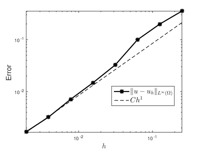
Figure 7.1. Example 1: smooth solution $u$ and anisotropic $A$ with aspect ratio $5$. The choice $\epsilon=\frac{1}{2}\sqrt{h}$ yields a linear asymptotic rate which is consistent with both Corollary 6.8 and Remark 6.1.

We point out that on average, it takes about $30\%$ of the computing time to assemble the matrix, mostly due to the FELICITY search routine to evaluate second differences. It takes about $50\%$ of the computing time to solve the (non-symmetric) linear systems using MATLAB backslash. However, solving the system requires significantly more time than assembling the matrix for finer meshes. The finest meshsize is $h=2^{-9}$, which corresponds to about $2.6\times 10^{5}$ degrees of freedom and a relative pointwise error of about $0.3\,\%$.

7.3. Example 2: discontinuous coefficients

Let $\Omega=[-1,1]^{2}$, the coefficient matrix $A$ exhibit the checkerboard structure

(7.2) $$A(x,y)=\bigl{(}\begin{smallmatrix}2&1\\ 1&2\end{smallmatrix}\bigr{)}\quad\text{ if $xy>0$,}\qquad A(x,y)=\bigl{(}\begin{smallmatrix}2&-1\\ -1&2\end{smallmatrix}\bigr{)}\quad\text{ if $xy\leq 0$,}$$

with discontinuities across the axes, and the exact solution be given by

(7.3) $$u(x,y)=\phi(x)\phi(y)\quad\text{ where }\quad\phi(x)=(xe^{1-|x|}-x).$$

A simple calculation yields

$$\boldsymbol{\nabla}\phi(x)=\big{(}1-|x|\big{)}e^{1-|x|}-1\quad\text{and}\quad D^{2}\phi(x)=\big{(}x-2\,\text{sgn}(x)\big{)}e^{1-|x|}.$$

Since $u\in W^{3}_{\infty}(\Omega\setminus\Sigma),A\in W^{1}_{\infty}(\Omega\setminus\Sigma)$ with discontinuity set $\Sigma$ being the two coordinate axes, we can take $\alpha=1$, choose $\epsilon=0.5h^{4/5}$ and expect a convergence rate $2/5$ according to Corollary 6.9. Figure 7.2 (a) displays an experimental order of convergence approximately $0.74$, which is much higher than predicted.

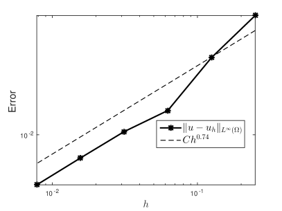
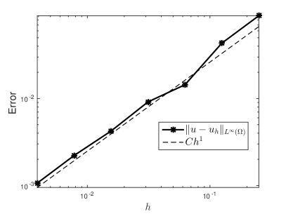
Figure 7.2. Example 2. The figure on the left shows that when $\epsilon=\frac{1}{2}h^{4/5}$, the convergence rate is $0.74$, better than the rate $2/5$ predicted in Corollary 6.9. The figure on the right shows that when $\epsilon=h^{1/2}$, the convergence rate is $1$. This example shows that the discrete ABP estimate may overestimate the $L^{\infty}$-error when $D^{2}u$ is discontinuous.

The finest meshsize is $h=2^{-7}$, which corresponds to about $6.5\times 10^{4}$ degrees of freedom and a relative pointwise accuracy of about $1.3\,\%$.

To explain this better convergence rate, we note that the consistency error

$$E_{h}^{\epsilon}(x_{i}):=f_{i}-L_{h}^{\epsilon}I_{h}u(x_{i})=L_{h}^{\epsilon}[u_{h}^{\epsilon}-I_{h}u](x_{i})$$

is concentrated along the $x$ and $y$-axis, where $I_{h}u$ is the piecewise linear interpolant of $u$ on mesh ${\mathcal{T}_{h}}$. We have found computationally that the error $e_{h}^{\epsilon}:=u^{\epsilon}_{h}-I_{h}u$ changes rapidly (of order $O(1)$) in the direction perpendicular to $\Sigma$ and smoothly (of order $O(h^{2})$) along $\Sigma$. In fact, if node $x_{i}$ belongs to the $y$-axis, we observe

(7.4) $$\frac{\big{|}\delta e_{h}^{\epsilon}(x_{i},hv_{1})\big{|}}{h^{2}}=O(1),\quad\frac{\big{|}\delta e_{h}^{\epsilon}(x_{i},hv_{2})\big{|}}{h^{2}}=O(h^{2}).$$

where $v_{1}=(1,0)$ and $v_{2}=(0,1)$. We see a similar behavior with $v_{1}$ and $v_{2}$ exchanged if $x_{i}$ belongs to the $x$-axis. We believe that the discrete ABP estimate of Theorem 5.1 overestimates the pointwise error in this case.

In order to give a plausible explanation, we start with Proposition 5.1 (discrete Alexandroff estimate) applied to $e_{h}^{\epsilon}$

(7.5) $$\sup_{\Omega}\,(e_{h}^{\epsilon})^{-}\leq C\left(\sum_{x_{i}\in\mathcal{C}_{h}^{-}(e_{h}^{\epsilon})}|\boldsymbol{\nabla}e_{h}^{\epsilon}(x_{i})|\right)^{1/2}.$$

Applying the definition of sub-differential, we deduce $\boldsymbol{\nabla}e_{h}^{\epsilon}(x_{i})\subset R(x_{i})$ where

$$R(x_{i})=\{w\in\mathbb{R}^{d}, \;\pm w\cdot hv_{1}\leq e_{h}^{\epsilon}(x_{i}\pm hv_{1})-e_{h}^{\epsilon}(x_{i})$$

and $$\;\pm w\cdot hv_{2}\leq e_{h}^{\epsilon}(x_{i}\pm hv_{2})-e_{h}^{\epsilon}(x_{i})\}$$

It is easy to check that $|R(x_{i})|=\frac{\big{|}\delta e_{h}^{\epsilon}(x_{i},hv_{1})\big{|}\,\big{|}\delta e_{h}^{\epsilon}(x_{i},hv_{2})\big{|}}{h^{2}}$ which yields

$$|\boldsymbol{\nabla}e_{h}^{\epsilon}(x_{i})|\leq\frac{\big{|}\delta e_{h}^{\epsilon}(x_{i},hv_{1})\big{|}\,\big{|}\delta e_{h}^{\epsilon}(x_{i},hv_{2})\big{|}}{h^{2}}.$$

Hence, since $|\omega_{i}|\approx h^{2}$ for $d=2$, (7.5) yields

$$\sup_{\Omega}\,(e_{h}^{\epsilon})^{-}\leq C\left(\sum_{x_{i}\in\mathcal{C}_{h}^{-}(e_{h}^{\epsilon})}\left(\frac{\delta e_{h}^{\epsilon}(x_{i},hv_{1})}{h^{2}}+\frac{\delta e_{h}^{\epsilon}(x_{i},hv_{2})}{h^{2}}\right)^{2}|\omega_{i}|\right)^{1/2},$$

because $\delta e_{h}^{\epsilon}(x_{i},hv_{j})\geq 0$ for $x_{i}\in\mathcal{C}_{h}^{-}(e_{h}^{\epsilon})$ and $j=1,2$. We deal with meshes ${\mathcal{T}_{h}}$ for which the discrete Laplacian satisfies $\Delta_{h}v_{h}(x_{i})=\frac{\delta v_{h}(x_{i},hv_{1})}{h^{2}}+\frac{\delta v_{h}(x_{i},hv_{2})}{h^{2}}$ for any piecewise linear function $v_{h}$; see Remark 7.1. Consequently,

$$\sup_{\Omega}\,(e_{h}^{\epsilon})^{-}\leq C\left(\sum_{x_{i}\in\mathcal{C}_{h}^{-}(e_{h}^{\epsilon})}(\Delta_{h}e_{h}^{\epsilon}(x_{i}))^{2}|\omega_{i}|\right)^{1/2}\leq C\left(\sum_{x_{i}\in\mathcal{C}_{h}^{-}(e_{h}^{\epsilon})}(L_{h}^{\epsilon}e_{h}^{\epsilon}(x_{i}))^{2}|\omega_{i}|\right)^{1/2}.$$

Applying (7.4) gives

$$\Delta_{h}e_{h}^{\epsilon}(x_{i})=\frac{\delta e_{h}^{\epsilon}(x_{i},hv_{1})}{h^{2}}+\frac{\delta e_{h}^{\epsilon}(x_{i},hv_{2})}{h^{2}}=O(1)$$

and

$$\frac{\delta e_{h}^{\epsilon}(x_{i},hv_{1})}{h^{2}}\frac{\delta e_{h}^{\epsilon}(x_{i},hv_{2})}{h^{2}}=O(h^{2})$$

for nodes $x_{i}\in\Sigma_{\epsilon}\cap\mathcal{C}_{h}^{-}(e_{h}^{\epsilon})$, where $\Sigma_{\epsilon}$ is defined in (6.18). Therefore, setting $\mathcal{C}_{h}^{-}:=\mathcal{C}_{h}^{-}(e_{h}^{\epsilon})$ and accounting for the correct contribution of $\Sigma_{\epsilon}$, (7.5) implies

$$\Big{|}\sup_{\Omega}\,(e_{h}^{\epsilon})^{-}\Big{|}^{2} \leq C\sum_{x_{i}\in\mathcal{C}_{h}^{-}\setminus\Sigma_{\epsilon}}(L_{h}^{\epsilon}e_{h}^{\epsilon}(x_{i}))^{2}|\omega_{i}|$$

$$+C\sum_{x_{i}\in\mathcal{C}_{h}^{-}\cap\Sigma_{\epsilon}}\frac{\delta e_{h}^{\epsilon}(x_{i},hv_{1})}{h^{2}}\frac{\delta e_{h}^{\epsilon}(x_{i},hv_{2})}{h^{2}}|\omega_{i}|\leq\;C\left(\Big{(}\epsilon^{2}+\frac{h^{2}}{\epsilon^{2}}\Big{)}^{2}+h^{2}\epsilon\right),$$

while the discrete ABP estimate overestimates $\sup_{\Omega}\,(e_{h}^{\epsilon})^{-}$. If we now choose $\epsilon=\sqrt{h}$, then the rate of convergence is order $h$ which is consistent with Figure 7.2 (b) The finest meshsize in such figure is $h=2^{-8}$, which leads to about $2.6\times 10^{5}$ degrees of freedom and a pointwise relative error of about $0.4\,\%$.

7.4. Example 3: $C^{2,\alpha}$-solution and $C^{0,\alpha}$-coefficients

We finally consider $\Omega=(-1,1)^{2}$ and the following solution $u$ and coefficient matrix $A$

(7.6) $$u(x)=|x|^{2+\alpha}\quad\text{ and }\quad A(x)=I+|x|^{\alpha}\frac{x}{|x|}\otimes\frac{x}{|x|}$$

with $0<\alpha<1$; we choose $\alpha=0.4$. Since $u\in C^{2,\alpha}(\overline{\Omega})$ and $A\in C^{0,\alpha}(\overline{\Omega})$, we take $\epsilon=1.5h^{2/(2+\alpha)}$, and expect a convergence rate $O(h^{2\alpha/(2+\alpha)})=O(h^{1/3})$ according to Corollary 6.7. This prediction is verified in Figure 7.3 (a) which shows an approximate rate $1/3$. The finest meshsize is $h=2^{-8}$, which gives rise to about $2.6\times 10^{5}$ degrees of freedom and a relative pointwise accuracy of about $2.3\,\%$.

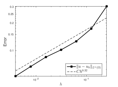
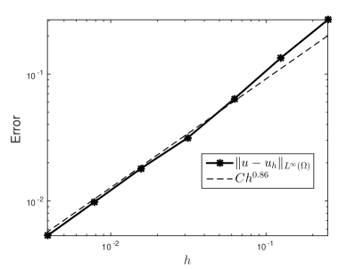
Figure 7.3. Example 3: $C^{2,\alpha}$-solution and $C^{0,\alpha}$-coefficients. (a) If $\epsilon=1.5h^{2/(2+\alpha)}$, then the convergence rate is $1/3$, which is consistent with Corollary 6.7. (b) If $\epsilon=1.5h^{2/(3+\alpha)}$, then the convergence rate is about $0.86$, which is better but is not supported by $C^{2,\alpha}$-regularity of $u$.

The error $u_{h}^{\epsilon}-u_{G}$ in the $L^{\infty}$-norm is bounded by the operator consistency error

$$E_{h}^{\epsilon}(x_{i}):=f_{i}-L_{h}^{\epsilon}u_{G}(x_{i})=L_{h}^{\epsilon}[u_{h}^{\epsilon}-u_{G}](x_{i})$$

in the discrete $L^{d}$-norm, according to Theorem 5.1 (discrete ABP estimate). Since $u\in H^{3+\alpha}(\Omega)$ and $d=2$, we conjecture that the quantity

$$\left(\sum_{x_{i}\in{\mathcal{N}_{h}}}\big{|}E_{h}^{\epsilon}(x_{i})\big{|}^{2}|\omega_{i}|\right)^{1/2}=O\left(\epsilon^{1+\alpha}+\frac{h^{2}}{\epsilon^{2}}\right),$$

dictates the pointwise convergence rate of $u-u^{\epsilon}_{h}$. Assuming this behavior, choosing $\epsilon=O(h^{2/(3+\alpha)})$, and applying Theorem 5.1, we deduce

$$\|\,u-u^{\epsilon}_{h}\,\|_{L^{\infty}(\Omega)}\leq O(h^{\frac{2+2\alpha}{3+\alpha}})\approx O(h^{0.82})$$

which is faster than the rate from Corollary 6.7. In Figure 7.3 (b), we observe that the computational order of convergence is about $0.86$, which confirms this heuristic explanation; we are currently exploring this issue [44]. The finest meshsize in Figure 7.3 (b) is $h=2^{-8}$, which leads to about $2.6\times 10^{5}$ degrees of freedom and a pointwise relative accuracy of about $0.23\,\%$.

Acknowledgements: We would like to thank L. Caffarelli for bringing up the integro-differential approach of [11] to us, as well as C. Gutierrez for mentioning the discrete ABP estimate of [34]. We would also like to thank Tengfei Su for implementing the two-scale method and the referees for their incisive comments and suggestions which led to a much better exposition of techniques and results.

References

- [1] G. Barles and E. R. Jakobsen. Error bounds for monotone approximation schemes for Hamilton-Jacobi-Bellman equations. SIAM J. Numer. Anal., 43(2):540–558 (electronic), 2005.
- [2] G. Barles and P. E. Souganidis. Convergence of approximation schemes for fully nonlinear second order equations. Asymptotic Anal., 4:271–283, 1991.
- [3] S. Bartels. Stability and convergence of finite-element approximation schemes for harmonic maps. SIAM J. Numer. Anal., 43(1):220–238 (electronic), 2005.
- [4] J.-D. Benamou, B. D. Froese and A. M. Oberman. Numerical solution of the optimal transportation problem using the Monge-Ampère equation. J. Comput. Phys., 260:107–126, 2014.
- [5] S. N. Bernstein. Sur la généralisation du probléme de Dirichlet. Math. Ann., 62:253–271, 1906; 69:82-136. 1910.
- [6] J. F. Bonnans and H. Zidani. Consistency of generalized finite difference schemes for the stochastic HJB equation. SIAM J. Numer. Anal., 41(3):1008–1021, 2003.
- [7] S. Brenner and L.R. Scott. The Mathematical Theory of Finite Element Methods. Springer 2014.
- [8] L. Caffarelli. Elliptic second order equations. Rend. Sem. Mat. Fis. Milano, 58:253–284 (1990), 1988.
- [9] L. Caffarelli and X. Cabré. Fully nonlinear elliptic equations, volume 43 of American Mathematical Society Colloquium Publications. American Mathematical Society, Providence, RI, 1995.
- [10] L. Caffarelli, M.G. Crandall, M. Kocan, and A. Świech, On viscosity solutions of fully nonlinear equations with measurable ingredients. Comm. Pure Appl. Math., 1996.
- [11] L. Caffarelli and L. Silvestre. Smooth approximations of solutions to nonconvex fully nonlinear elliptic equations. In Nonlinear partial differential equations and related topics, volume 229, pages 67–85. Amer. Math. Soc., Providence, RI, 2010.
- [12] L. Caffarelli and P. E. Souganidis. A rate of convergence for monotone finite difference approximations to fully nonlinear, uniformly elliptic PDEs. Comm. Pure Appl. Math., 61:1–17, 2008.
- [13] F. Camilli and M. Falcone. An approximation scheme for the optimal control of diffusion processes. RAIRO Modél. Math. Anal. Numér., 29(1):97–122, 1995.
- [14] Ph. Ciartet and P.A. Raviart. Maximum principle and uniform convergence for the finite element method. Comp. Meths. Appl. Mech. Eng., 2(1):17–-31. 1973.
- [15] F. Chiarenza, M. Frasca, and P. Longo. Interior estimates for nondivergence elliptic equations with discontinuous coefficients. Ricerche Mat., 40(1):149–168, 1991.
- [16] F. Chiarenza, M. Frasca, and P. Longo. -solvability of the Dirichlet problem for nondivergence elliptic equations with VMO coefficients. Trans. Amer. Math. Soc., 336(2):841–853, 1993.
- [17] P. G. Ciarlet. Basic error estimates for elliptic problems. In Handbook of numerical analysis, Vol. II, Handb. Numer. Anal., II, pages 17–351. North-Holland, Amsterdam, 1991.
- [18] E. J. Dean and R. Glowinski. Numerical solution of the two-dimensional elliptic Monge-Ampère equation with Dirichlet boundary conditions: an augmented Lagrangian approach. C. R. Math. Acad. Sci. Paris, 336(9):779–784, 2003.
- [19] K. Debrabant and E. R. Jakobsen. Semi-Lagrangian schemes for linear and fully non-linear diffusion equations. Math. Comp., 82(283):1433–1462, 2013.
- [20] X. Feng, L. Hennings, and M. Neilan. Finite element methods for second order linear elliptic partial differential equations in non-divergence form. Math. Comp., (to appear).
- [21] W. H. Fleming and H. M. Soner. Controlled Markov processes and viscosity solutions, volume 25 of Stochastic Modelling and Applied Probability. Springer, New York, second edition, 2006.
- [22] D. Gilbarg and N. S. Trudinger. Elliptic partial differential equations of second order, volume 224 of Grundlehren der Mathematischen Wissenschaften [Fundamental Principles of Mathematical Sciences]. Springer-Verlag, Berlin, second edition, 1983.
- [23] B. Grünbaum. Convex polytopes, volume 221 of Graduate Texts in Mathematics. Springer-Verlag, New York, second edition, 2003. Prepared and with a preface by Volker Kaibel, Victor Klee and Günter M. Ziegler.
- [24] Q. Han and F. Lin. Elliptic partial differential equations, volume 1 of Courant Lecture Notes in Mathematics. New York University, Courant Institute of Mathematical Sciences, New York; American Mathematical Society, Providence, RI, 1997.
- [25] R. R. Jensen. Uniformly elliptic PDEs with bounded, measurable coefficients. J. Fourier Anal. Appl., 2(3):237–259, 1995.
- [26] M. Jensen and I. Smears. On the convergence of finite element methods for Hamilton-Jacobi-Bellman equations. SIAM J. Numer. Anal., 51(1):137–162, 2013.
- [27] D. Kim. Second order elliptic equations in with piecewise continuous coefficients. Potential Anal., 26:189–212, 2007.
- [28] M. Kocan. Approximation of viscosity solutions of elliptic partial differential equations on minimal grids Numer. Math., 72:73–92, 1995.
- [29] S. Korotov, M. Křížek, and P. Neittaanmäki. Weakened acute type condition for tetrahedral triangulations and the discrete maximum principle. Math. Comp., 70(233):107–119 (electronic), 2001.
- [30] N. V. Krylov. On the rate of convergence of finite-difference approximations for Bellman’s equations. Algebra i Analiz, 9:245–256, 1997.
- [31] N. V. Krylov. On the rate of convergence of finite-difference approximations for Bellman’s equations with variable coefficients. Probab. Theory Related Fields, 117:1–16, 2000.
- [32] A. Kufner, O. John, and S. Fučík. Function spaces. Noordhoff International Publishing, Leyden; Academia, Prague, 1977. Monographs and Textbooks on Mechanics of Solids and Fluids; Mechanics: Analysis.
- [33] H. J. Kuo and N. S. Trudinger. Discrete methods for fully nonlinear elliptic equations. SIAM J. Numer. Anal., 29:123–135, 1992.
- [34] H-J. Kuo and N. S. Trudinger. A note on the discrete Aleksandrov-Bakelman maximum principle. In Proceedings of 1999 International Conference on Nonlinear Analysis (Taipei), volume 4, pages 55–64, 2000.
- [35] H. J. Kushner and P. Dupuis. Numerical methods for stochastic control problems in continuous time, volume 24 of Applications of Mathematics (New York). Springer-Verlag, New York, second edition, 2001. Stochastic Modelling and Applied Probability.
- [36] O. A. Ladyzhenskaya and N. N. Ural′tseva. Linear and quasilinear elliptic equations. Translated from the Russian by Scripta Technica, Inc. Translation editor: Leon Ehrenpreis. Academic Press, New York-London, 1968.
- [37] O. Lakkis and T. Pryer. A finite element method for second order nonvariational elliptic problems. SIAM J. Sci. Comput., 33(2):786–801, 2011.
- [38] A. Lorenzi. On elliptic equations with piecewise constant coefficients, II. Ann. Scuola Norm. Sup. Pisa, 26(3), 839–-870, 1972.
- [39] A. Maugeri, D. K. Palagachev, and L. G. Softova. Elliptic and parabolic equations with discontinuous coefficients, volume 109 of Mathematical Research. Wiley-VCH Verlag Berlin GmbH, Berlin, 2000.
- [40] T. S. Motzkin and W. Wasow. On the approximation of linear elliptic differential equations by difference equations with positive coefficients. J. Math. Physics, 31:253–59, 1953.
- [41] N. Nadirashvili. Nonuniqueness in the martingale problem and the Dirichlet problem for uniformly elliptic operators. Ann. Scuola Norm. Sup. Pisa Cl. Sci. (4), 24(3):537–549, 1997.
- [42] R. H. Nochetto, M. Paolini, and C. Verdi. An adaptive finite element method for two-phase Stefan problems in two space dimensions. I. Stability and error estimates. Math. Comp., 57(195):73–108, S1–S11, 1991.
- [43] R. H. Nochetto and W. Zhang. Pointwise rates of convergence for the Oliker-Prussner method for the Monge-Ampère equation. (submitted).
- [44] R. H. Nochetto and W. Zhang. Two-scale FEM for equations in non-divergence form: Calderón-Zygmund theory. (in preparation).
- [45] M. Safonov. Nonuniqueness for second-order elliptic equations with measurable coefficients. SIAM J. Math. Anal., 30(4):879–895 (electronic), 1999.
- [46] A. H. Schatz and L. B. Wahlbin. On the quasi-optimality in of the -projection into finite element spaces. Math. Comp., 38(157):1–22, 1982.
- [47] I. Smears and E. Süli. Discontinuous Galerkin finite element approximation of nondivergence form elliptic equations with Cordès coefficients. SIAM J. Numer. Anal., 51(4):2088–2106, 2013.
- [48] I. Smears and E. Süli. Discontinuous Galerkin finite element approximation of Hamilton-Jacobi-Bellman equations with Cordès coefficients. SIAM J. Numer. Anal., 52(2):993–1016, 2014.
- [49] A. H. Stroud. Approximate calculation of multiple integrals. Prentice-Hall, Inc., Englewood Cliffs, N.J., 1971. Prentice-Hall Series in Automatic Computation.
- [50] S. Walker. FELICITY: Finite Element Implementation and Computational Interface Tool for you, Tutorial, 2013.
- [51] C. Wang and J. Wang. A primal-dual weak galerkin finite element method for second order elliptic equations in non-divergence form. http://arxiv.org/abs/1510.03499.