Electron Heating by the Ion Cyclotron Instability in Collisionless Accretion Flows.
II. Electron Heating Efficiency as a Function of Flow Conditions

Abstract

In the innermost regions of low-luminosity accretion flows, including Sgr A^∗ at the center of our Galaxy, the frequency of Coulomb collisions is so low that the plasma is two-temperature, with the ions substantially hotter than the electrons. This paradigm assumes that Coulomb collisions are the only channel for transferring the ion energy to the electrons. In this work, the second of a series, we assess the efficiency of electron heating by ion velocity-space instabilities in collisionless accretion flows. The instabilities are seeded by the pressure anisotropy induced by magnetic field amplification, coupled to the adiabatic invariance of the particle magnetic moments. Using two-dimensional (2D) particle-in-cell (PIC) simulations, we showed in Paper I that if the electron-to-ion temperature ratio is $T_{0e}/T_{0i}\lesssim 0.2$, the ion cyclotron instability is the dominant mode for ion betas $\beta_{0i}\sim 5-30$ (here, $\beta_{0i}$ is the ratio of ion thermal pressure to magnetic pressure), as appropriate for the midplane of low-luminosity accretion flows. In this work, we employ analytical theory and 1D PIC simulations (with the box aligned with the fastest growing wavevector of the ion cyclotron mode) to fully characterize how the electron heating efficiency during the growth of the ion cyclotron instability depends on the electron-to-proton temperature ratio, the plasma beta, the Alfvén speed, the amplification rate of the mean field (in units of the ion Larmor frequency) and the proton-to-electron mass ratio. Our findings can be incorporated as a physically-grounded sub-grid model into global fluid simulations of low-luminosity accretion flows, thus helping to assess the validity of the two-temperature assumption.

1. Introduction

In low-luminosity accretion flows, including the ultra-low-luminosity source Sagittarius A^∗ (Sgr A^∗) at our Galactic Center (Narayan et al., 1995, 1998; Yuan et al., 2003; Xu et al., 2006; Mościbrodzka et al., 2012; Yuan & Narayan, 2014), the timescale for electron and ion Coulomb collisions is much longer than the inflow time in the disk, i.e., the plasma is collisionless. At distances less than a few hundred Schwarzschild radii from the black hole ($R_{S}\equiv 2\,GM_{\bullet}/c^{2}$ is the Schwarzschild radius, where $M_{\bullet}$ is the black hole mass), ions and electrons are thermally decoupled and the plasma is two-temperature, with the ions substantially hotter than the electrons (Narayan & Yi, 1995; Yuan et al., 2003). This stems from the fact that (i) compressive heating favors non-relativistic ions over relativistic electrons, and that (ii) electrons copiously lose energy via radiative cooling.

Early work on two-temperature models of low-luminosity accretion flows (also known as ADAFs, or advection-dominated accretion flows) assumed that most of the turbulent viscous energy goes into the ions (Ichimaru, 1977; Rees et al., 1982; Narayan & Yi, 1995), and that only a small fraction $\sim 10^{-3}-10^{-2}$ goes into the electrons. There have been occasional attempts to estimate this fraction from microphysics, by considering magnetic reconnection (Bisnovatyi-Kogan & Lovelace, 1997; Quataert & Gruzinov, 1999), magnetohydrodynamic (MHD) turbulence (Quataert, 1998; Blackman, 1999; Medvedev, 2000), plasma waves (Begelman & Chiueh, 1988), or dissipation of pressure anisotropy in collisionless plasmas (Sharma et al., 2007). Currently, it appears that the electron-to-proton temperature ratio lies in the range $0.1-0.5$, but this is by and large no more than a guess (Narayan & Yi, 1995; Yuan et al., 2003; Yuan & Narayan, 2014). The micro-physics of energy dissipation and electron heating in collisionless accretion flows cannot be captured in the MHD framework, but it requires a fully-kinetic description with first-principles particle-in-cell (PIC) simulations.

In this work, the second of a series, we study with PIC simulations the efficiency of electron heating by ion velocity-space instabilities, in the context of low-luminosity accretion disks. Pressure anisotropies are continuously generated in collisionless accretion flows due to the fluctuating magnetic fields associated with the non-linear stages of the magnetorotational instability (MRI, Balbus & Hawley 1991, 1998), a MHD instability that governs the transport of angular momentum in accretion disks (see Riquelme et al., 2012; Hoshino, 2013, for a study of the collisionless MRI). If the magnetic field is amplified by the MRI, the adiabatic invariance of the magnetic moments of charged particles drives the perpendicular (to the magnetic field) pressure $P_{\perp}$ to be much greater than the parallel pressure $P_{\parallel}$, a configuration prone to velocity-space instabilities. The same instabilities are believed to play an important role in the solar wind (Kasper et al., 2002, 2006; Bale et al., 2009; Maruca et al., 2011, 2012; Matteini et al., 2007, 2013; Cranmer et al., 2009; Cranmer & van Ballegooijen, 2012) and in the intracluster medium (Schekochihin et al., 2005; Lyutikov, 2007; Santos-Lima et al., 2014).

In Paper I, we have developed a fully-kinetic method for studying velocity-space instabilities in a system where the field is continuously amplified. In this case, the anisotropy is constantly driven (as a result of the field amplification), rather than assumed as a prescribed initial condition, as in most earlier works (see Gary, 1993, for a review). In our setup, the increase in magnetic field is driven by compression (as in Hellinger & Trávníček, 2005), mimicking the effect of large-scale compressive motions in ADAFs. However, our results hold regardless of what drives the field amplification, so they can be equally applied to the case where velocity-space instabilities are induced by incompressible shear motions (as in Riquelme et al., 2014; Kunz et al., 2014).

Most of the previous numerical studies of anisotropy-driven instabilities focused either on ion instabilities alone (with hybrid codes, see Gary 1993; Hellinger et al. 2006 for a review; or fully-kinetic simulations in electron-positron plasmas, Riquelme et al. 2014) or on electron modes alone (keeping the ions as a static neutralizing background, see Gary 1993 for a review). Neither approach can capture self-consistently the energy transfer from ions to electrons, which requires fully-kinetic simulations with mobile ions and a realistic mass ratio. This is the purpose of our work.

With fully-kinetic PIC simulations, we study the efficiency of electron heating that results from ion velocity-space instabilities driven by magnetic field amplification in collisionless accretion flows. We focus on the regime $T_{0e}/T_{0i}\lesssim 0.2$ (here, $T_{0e}$ and $T_{0i}$ are the electron and ion temperatures, respectively) where, as demonstrated in Paper I, the dominant mode is the ion cyclotron instability (e.g., Gary et al., 1976, 1993; Hellinger et al., 2006), rather than the mirror instability (e.g., Hasegawa, 1969; Southwood & Kivelson, 1993; Kivelson & Southwood, 1996). Since the wavevector of the ion cyclotron instability is along the mean magnetic field, the relevant physics can be conveniently studied by means of 1D simulations, with the box aligned with the ordered field. Via 1D PIC simulations, we assess here the dependence of the electron heating efficiency on the initial ratio between electron and proton temperatures, the ion beta $\beta_{0i}$ (namely, the ratio of ion thermal pressure to magnetic pressure), the Alfvén speed, the amplification rate of the mean field (in units of the ion Larmor frequency) and the proton-to-electron mass ratio. Eqs. (26)-(28) emphasize how the various contributions to electron heating depend on the flow conditions. Their sum gives the overall electron energy gain due to the growth of the ion cyclotron instability, and it represents the main result of this paper.

This work is organized as follows. In Section 2, we describe the physical conditions in the innermost regions of low-luminosity accretion flows, where the plasma is believed to be two-temperature. The setup of our simulations is discussed in Section 3. Section 4 summarizes the conclusions of Paper I and anticipates the main results of this work (consisting of Eqs. (26)-(28)), which are extensively substantiated by our findings in Section 5. We discuss the astrophysical implications of our work in Section 6.

2. Physical Conditions in Accretion Disks

For our investigation of velocity-space instabilities in collisionless accretion flows, we employ values of the ion temperature $T_{0i}$, the ion beta $\beta_{0i}=8\pi n_{0}k_{B}T_{0i}/B_{0}^{2}$ and the Alfvén velocity $v_{A0i}=B_{0}/\sqrt{4\pi n_{0}m_{i}}$ that are consistent with estimates taken from state-of-the-art general-relativistic magnetohydrodynamic (GRMHD) simulations of Sgr A^∗, the low-luminosity accretion flow at our Galactic Center (e.g., Sa̧dowski et al., 2013). Here, $n_{0}$ and $B_{0}$ are the ion number density and the magnetic field strength, respectively.

GRMHD simulations can successfully describe the linear and non-linear evolution of the MRI. Yet, they cannot properly capture the dissipation of MRI-driven turbulence on small scales (the electron Larmor radius), which ultimately regulates the temperature balance between protons and electrons, in the innermost regions of ADAFs where the plasma is two-temperature. It follows that GRMHD simulations cannot predict the value of the electron-to-proton temperature ratio $T_{0e}/T_{0i}$ to be employed in our PIC experiments, so we will have to study the dependence of our results on this parameter.

We estimate the values of $T_{0i}$, $\beta_{0i}$ and $v_{A0i}$ in the innermost regions of ADAFs (at distances less than a few hundred Schwarzschild radii from the black hole) from Fig. 1 of Sa̧dowski et al. (2013). The ion temperature decreases with distance from the black hole as $R^{-1}$, from $T_{0i}\sim 10^{11.5}\nobreak{\mathrm{\;K}}$ at the innermost stable circular orbit ($R_{\rm ISCO}=3\,R_{S}$, for a non-rotating black hole) down to $T_{0i}\sim 10^{10}\nobreak{\mathrm{\;K}}$ at $R\sim 100\,R_{S}$. In units of the proton rest mass energy, it varies in the range $k_{B}T_{0i}/m_{i}c^{2}\sim 0.001-0.03$, i.e., the ions are non-relativistic. On the other hand, if the electrons were to be in equipartition with the ions, they would have $k_{B}T_{0e}/m_{e}c^{2}\sim 1.8-50$, i.e., the electrons can be relativistically hot.

The ion beta is nearly constant with radius, and along the disk midplane it ranges from $\beta_{0i}\sim 10$ to $\beta_{0i}\sim 30$ (Fig. 1 of Sa̧dowski et al. (2013)). Lower values of the plasma beta are expected at high latitudes above and below the disk, in the so-called corona, where the plasma might be magnetically dominated (i.e., $\beta_{0i}\ll 1$). In this work, we only focus on velocity-space instabilities triggered in the bulk of the disk, and we take $\beta_{0i}=5$ as the lowest value we consider, arguing that our results can be applied all the way down to $\beta_{0i}\sim 1$. We extend our investigation to higher values of $\beta_{0i}$, up to $80$. Most likely, this is not directly relevant for low-luminosity accretion flows, but it might have important implications for the physics of the intracluster medium (Schekochihin et al., 2005; Lyutikov, 2007; Santos-Lima et al., 2014).

The value of the Alfvén velocity can be derived from the ion temperature and the ion beta, since $v_{A0i}/c=\sqrt{2k_{B}T_{0i}/\beta_{0i}m_{i}c^{2}}$. It follows that the Alfvén speed varies in the range $v_{A0i}/c\sim 0.01-0.1$, if $k_{B}T_{0i}/m_{i}c^{2}\sim 0.001-0.03$ and $\beta_{0i}\sim 10-30$. Below, we show that our results are not sensitive to variations in the Alfvén velocity, in the range $v_{A0i}/c\sim 0.025-0.1$ that we explore.

To fully characterize our system, we need to specify the rate $q$ of magnetic field amplification, in units of the ion gyration frequency $\omega_{0ci}=eB_{0}/m_{i}c$. In accretion flows, we expect the ratio $\omega_{0ci}/q$ to be much larger than unity ($\sim 10^{7}$, if $q$ is comparable to the local orbital frequency). For computational convenience, we employ smaller values of $\omega_{0ci}/q$, exploring the range $\omega_{0ci}/q=50-3200$, and we show that our results converge in the limit $\omega_{0ci}/q\gg 1$.

Also, due to computational constraints, fully-kinetic PIC simulations are forced to employ a reduced value of the ion-to-electron mass ratio (e.g., Riquelme et al. 2014 primarily studied velocity-space instabilities in electron-positron plasmas, i.e., with $m_{e}=m_{i}$). Most of our results employ a reduced mass ratio ($m_{i}/m_{e}=16$ or 64). However, we show that our conclusions can be readily rescaled up to realistic mass ratios (we extend our study up to $m_{i}/m_{e}=1024$). This is extremely important for low-luminosity accretion disks, since only with a realistic mass ratio one can describe the case of non-relativistic ions and ultra-relativistic electrons that is of particular interest for ADAF models.

3. Simulation Setup

We investigate electron heating due to ion velocity-space instabilities in collisionless accretion flows by means of fully-kinetic PIC simulations. We have modified the three-dimensional (3D) electromagnetic PIC code TRISTAN-MP (Buneman, 1993; Spitkovsky, 2005; Sironi et al., 2013; Sironi & Spitkovsky, 2014; Sironi & Giannios, 2014) to account for the effect of an overall compression of the system. Our model is complementary to the technique described in Riquelme et al. (2012) and employed in Riquelme et al. (2014), which is appropriate for incompressible shear flows.

Our method, the first of its kind for fully-kinetic PIC simulations of compressing systems, has been extensively described in Paper I (there, see Section 2 and Appendix A). For completeness, we report here its main properties. We solve Maxwell’s equations and the Lorentz force in the fluid comoving frame, which is related to the laboratory frame by a Lorentz boost. In the comoving frame, we define two sets of spatial coordinates, with the same time coordinate. The unprimed coordinate system has a basis of unit vectors, so it is the appropriate coordinate set to measure all physical quantities. Yet, we find it convenient to re-define the unit length of the spatial axes in the comoving frame such that a particle subject only to compression stays at fixed coordinates. This will be our primed coordinate system.

The location of a particle in the laboratory frame (identified by the subscript “L”) is related to its position in the primed coordinate system of the fluid comoving frame by $\mbox{\boldmath{$x$}}_{\rm L}=\mbox{\boldmath{$L$}}\,\mbox{\boldmath{$x$}}^{\prime}$, where compression is accounted for by the diagonal matrix

$$\mbox{\boldmath{${L}$}}=\frac{\partial\mbox{\boldmath{$x$}}}{\partial\mbox{\boldmath{$x$}}^{\prime}}=\left(\begin{array}[]{ccc}1&0&0\\ 0&(1+q\,t)^{-1}&0\\ 0&0&(1+q\,t)^{-1}\\ \end{array}\right)~{}~{}~{},$$ (4)

which describes compression along the $y$ and $z$ axes. By defining the determinant $\ell={\rm det}(\mbox{\boldmath{${L}$}})=(1+q\,t)^{-2}$, the two evolutionary Maxwell’s equations of the PIC method in a compressing box are, in the limit $|\dot{\mbox{\boldmath{${L}$}}}\,\mbox{\boldmath{$x$}}^{\prime}|/c\ll 1$ of non-relativistic compression speeds,

$$\nabla^{\prime}\times(\mbox{\boldmath{${L}$}}\mbox{\boldmath{$E$}}) = -\frac{1}{c}\frac{\partial}{\partial t^{\prime}}(\ell\,\mbox{\boldmath{$L$}}^{-1}\mbox{\boldmath{$B$}})~{}~{},$$ (5)

$$\nabla^{\prime}\times(\mbox{\boldmath{${L}$}}\mbox{\boldmath{$B$}}) = \frac{1}{c}\frac{\partial}{\partial t^{\prime}}(\ell\,\mbox{\boldmath{$L$}}^{-1}\mbox{\boldmath{$E$}})+\frac{4\pi}{c}\ell\,\mbox{\boldmath{$J$}}^{\prime}~{}~{},$$ (6)

where the temporal and spatial derivatives pertain to the primed coordinate system (the reader is reminded that the primed and unprimed systems share the same time coordinate, so $\partial/\partial t^{\prime}=\partial/\partial t$, whereas the spatial derivatives differ: $\nabla^{\prime}=\mbox{\boldmath{${L}$}}\,\nabla$). We define $E$ and $B$ to be the physical electromagnetic fields measured in the unprimed coordinate system. The current density $\mbox{\boldmath{$J$}}^{\prime}$ is computed by summing the contributions of individual particles, as we specify in Appendix A of Paper I.

The equations describing the motion of a particle with charge $q$ and mass $m$ can be written, still in the limit $|\dot{\mbox{\boldmath{${L}$}}}\,\mbox{\boldmath{$x$}}^{\prime}|/c\ll 1$ of non-relativistic compression speeds, as

$$\frac{{\rm d}\mbox{\boldmath{$p$}}}{{\rm d}t^{\prime}} = -\,\dot{\mbox{\boldmath{${L}$}}}\mbox{\boldmath{${L}$}}^{-1}\mbox{\boldmath{$p$}}+q\left(\mbox{\boldmath{$E$}}+\frac{\mbox{\boldmath{$v$}}}{c}\times\mbox{\boldmath{$B$}}\right)~{}~{},$$ (7)

$$\frac{{\rm d}\mbox{\boldmath{$x^{\prime}$}}}{{\rm d}t^{\prime}} = \mbox{\boldmath{$v$}}^{\prime}~{}~{},$$ (8)

where $\dot{\mbox{\boldmath{${L}$}}}={\rm d}\mbox{\boldmath{${L}$}}/{\rm d}t$. The physical momentum $\mbox{\boldmath{$p$}}=\gamma m\mbox{\boldmath{$v$}}$ and velocity $v$ of the particle are measured in the unprimed coordinate system (here, $\gamma=1/\sqrt{1-(\mbox{\boldmath{$v$}}/c)^{2}}$ is the particle Lorentz factor). Yet, the particle velocity $\mbox{\boldmath{$v$}}^{\prime}$ entering Eq. (8) refers to the primed coordinate system, where $\mbox{\boldmath{$v$}}^{\prime}=\mbox{\boldmath{${L}$}}^{-1}\mbox{\boldmath{$v$}}$. Eqs. (7) and (8) hold for particles of arbitrary Lorentz factor.

A uniform ordered magnetic field $\mbox{\boldmath{$B$}}_{0}$ is initialized along the $x$ direction. As a result of compression, Eq. (5) dictates that it should grow in time as $\mbox{\boldmath{$B$}}=\mbox{\boldmath{$B$}}_{0}(1+q\,t)^{2}$, which is consistent with flux freezing (the particle density in the box increases at the same rate). From the Lorentz force in Eq. (7), the component of particle momentum aligned with the field does not change during compression, so $p_{\parallel}=p_{0\parallel}$, whereas the perpendicular momentum increases as $p_{\perp}=p_{0\perp}(1+q\,t)$. This is consistent with the conservation of the first ($\mu\propto p_{\perp}^{2}/|\mbox{\boldmath{$B$}}|$) and second ($J\propto p_{\parallel}|\mbox{\boldmath{$B$}}|/n$) adiabatic invariants.

Our computational method is implemented for 1D, 2D and 3D computational domains. We use periodic boundary conditions in all directions, assuming that the system is locally homogeneous, i.e., that gradients in the density or in the ordered field $\mbox{\boldmath{$B$}}_{0}$ are on scales larger than the box size. In Paper I, we have demonstrated that if the initial electron temperature is less than $\sim 20\%$ of the ion temperature, the wavevector of the dominant instability is aligned with the ordered magnetic field. It follows that the evolution of the dominant mode can be conveniently captured by means of 1D simulations with the computational box oriented along $x$, which we will be employing in this work. Yet, all three components of electromagnetic fields and particle velocities are tracked.

The focus of this work is to assess how the efficiency of electron heating depends on the properties of the flow. We vary the ion plasma beta

$$\beta_{0i}=\frac{8\pi n_{0}k_{B}T_{0i}}{B_{0}^{2}}~{}~{}~{},$$ (9)

from $\beta_{0i}=5$ up to 80. Here, $n_{0}$ is the particle number density at the initial time and $T_{0i}$ the initial ion temperature (ions, as well as electrons, are initialized with a Maxwellian distribution). The electron thermal properties are specified via the electron beta

$$\beta_{0e}=\frac{T_{0e}}{T_{0i}}\,\beta_{0i}~{}~{}.$$ (10)

We vary the ratio $\beta_{0e}/\beta_{0i}$ from $10^{-1}$ down to $10^{-3}$. The magnetization is quantified by the Alfvén speed

$$v_{A0i}=\frac{B_{0}}{\sqrt{4\pi m_{i}n_{0}}}~{}~{}~{},$$ (11)

so that the initial ion temperature equals $k_{B}T_{0i}=m_{i}\beta_{0i}v_{A0i}^{2}/2$. We will show that our results are the same when varying the Alfvén velocity from 0.025 up to 0.1, with $v_{A0i}/c=0.05$ being our reference choice.

The ion cyclotron frequency, which is related to the ion plasma frequency by $\omega_{0ci}=(v_{A0i}/c)\,\omega_{0\rm pi}$, will set the characteristic unit of time. In particular, we will scale the compression rate $q$ to be a fraction of the ion cyclotron frequency $\omega_{0ci}$. In accretion flows, we expect the ratio $\omega_{0ci}/q$ to be much larger than unity. We explore the range $\omega_{0ci}/q=50-3200$, showing that our results converge in the limit $\omega_{0ci}/q\gg 1$. We evolve the system up to a few compression timescales.

Since we are interested in capturing the efficiency of electron heating due to ion instabilities, we need to properly resolve the kinetic physics of both ions and electrons. We typically employ 32,768 computational particles per species per cell, but we have tested that our results are the same when using up to 131,072 particles per species per cell. Such large values are of critical importance to suppress the spurious heating induced by the coarse-grained description of PIC plasmas (e.g., Melzani et al., 2013), and so to reliably estimate the efficiency of electron heating by ion velocity-space instabilities, which is the primary focus of this work.

We resolve the electron skin depth $c/\omega_{0\rm pe}=\sqrt{c^{2}m_{e}/4\pi n_{0}e^{2}}\,$ with 5 cells, which is sufficient to capture the physics of the electron whistler instability (Kennel & Petschek, 1966; Ossakow et al., 1972b, a; Yoon & Davidson, 1987; Yoon et al., 2011). On the other hand, our computational domain needs to be large enough to include at least a few wavelengths of ion-driven instabilities, i.e., a few ion Larmor radii

$$r_{L,i}=\sqrt{\frac{3\,\beta_{0i}\,m_{i}}{2\,m_{e}}}\,\frac{c}{\omega_{0\rm pe}}~{}~{}.$$ (12)

Most of our results employ a reduced mass ratio ($m_{i}/m_{e}=16$ or 64), for computational convenience. However, we show that our conclusions can be readily rescaled up to realistic mass ratios (we extend our study up to $m_{i}/m_{e}=1024$). For $m_{i}/m_{e}=16$ and $\beta_{0i}=20$, which will be our reference case, we employ a 1D computational box with $L_{x}=1536\,{\rm cells}\sim 15\,r_{L,i}$. When changing $m_{i}/m_{e}$ or $\beta_{0i}$, we ensure that our computational domain is scaled such that it contains at least $\sim 10\,r_{L,i}$, so that the dominant wavelength of ion-driven instabilities is properly resolved.

4. Electron Heating by the Ion Cyclotron Instability

In this Section, we first summarize the main conclusions of Paper I. Then, we describe how the efficiency of electron heating depends on the flow conditions.

By means of 2D simulations, we have demonstrated in Paper I that, if the initial electron-to-ion temperature ratio is $T_{0e}/T_{0i}\lesssim 0.2$, the ion cyclotron instability dominates the relaxation of the ion anisotropy, over the competing mirror mode. Since the wavevector of the ion cyclotron instability is aligned with the mean magnetic field, the relevant physics can be conveniently studied by means of 1D simulations, with the box aligned with the ordered field. Thanks to the greater number of computational particles per cell allowed by 1D simulations, as opposed to 2D, the efficiency of electron heating by the ion cyclotron instability can be reliably estimated.

Since we are interested in the net heating of electrons by the ion cyclotron instability, and not in the straightforward effect of compression, we have chosen to quantify the efficiency of electron heating by defining the ratio

$$\chi\equiv\frac{m_{i}}{m_{e}}\frac{\langle p_{e}^{2}\rangle}{\langle p_{i}^{2}\rangle}~{}~{},$$ (13)

where $p_{e}=\gamma_{e}m_{e}v_{e}$ and $p_{i}=\gamma_{i}m_{i}v_{i}$ are the electron and ion momenta. The ratio $\chi$ remains constant before the growth of anisotropy-driven instabilities, since in a compressing box the particle parallel momentum does not change, whereas the perpendicular momentum increases as $p_{\perp}\propto(1+q\,t)$, so the total momentum $p=(p_{\parallel}^{2}+2\,p_{\perp}^{2})^{1/2}$ increases as $p=p_{0}\sqrt{[1+2\,(1+q\,t)^{2}]/3}$, for both electrons and ions. It follows that the $\chi$ parameter is a good indicator of the electron energy change occurring as a result of the ion cyclotron mode. The choice of the pre-factor $m_{i}/m_{e}$ is such that for non-relativistic particles, having $\langle p_{e}^{2}\rangle\simeq m_{e}^{2}\langle v_{e}^{2}\rangle$ and $\langle p_{i}^{2}\rangle\simeq m_{i}^{2}\langle v_{i}^{2}\rangle$, the parameter $\chi$ reduces to $\chi=m_{e}\langle v_{e}^{2}\rangle/m_{i}\langle v_{i}^{2}\rangle$, i.e., to the ratio of the average kinetic energies of electrons and ions.

As described in Paper I, the development of the ion cyclotron instability causes strong electron heating. The resulting change in the electron Lorentz factor $\langle\Delta\gamma_{e,q}\rangle$, averaged over all the electrons in the system, gives a corresponding increase in the $\chi$ parameter of

$$\Delta\chi\simeq\frac{m_{e}}{m_{i}}\frac{\langle\gamma_{e}\Delta\gamma_{e,q}\rangle c^{2}}{\langle\gamma_{i}^{2}v_{i}^{2}\rangle}~{}~{}~{},$$ (14)

where we have neglected higher order terms in $\Delta\gamma_{e,q}/\gamma_{e}\ll 1$, as we have motivated in Paper I. In turn, the mean energy gain $\langle\Delta\gamma_{e,q}m_{e}c^{2}\rangle$ at the end of the exponential growth of the ion cyclotron mode can be written as a sum of different terms (see Paper I)

$$\!\!\!\!\!\!\!\!\!\!\!\!\!\!\langle\Delta\gamma_{e,q}\rangle\equiv\langle\gamma_{e}-\gamma_{e,q}\rangle = \langle-|\Delta\gamma_{\rm curv}|+$$ (15)

$$+\Delta\gamma_{\partial B}\!+\!\Delta\gamma_{\nabla B}\!+\!\Delta\gamma_{E\times B}\rangle~{},$$

where we have subtracted $\gamma_{e,q}$ on the left hand side, since it describes the electron energy increase due to compression alone, which would be present even without any instability. The four terms on the right hand side of Eq. (15) can be written as a function of the plasma properties at the end of the exponential phase of ion cyclotron growth (as indicated by the subscript “exp” below)

$$\!\!\langle\Delta\gamma_{\partial B}\!-\!|\Delta\gamma_{\rm curv}|\rangle\! \simeq \!\left[\frac{k_{B}(T_{e\perp}-T_{e\parallel})}{m_{e}c^{2}}\,\frac{\langle\delta B_{\perp}^{2}\rangle}{2|\langle\mbox{\boldmath{$B$}}\rangle|^{2}}\right]_{\rm exp}$$ (16)

$$\!\!\langle\Delta\gamma_{\nabla B}\rangle\! \simeq \!\left[\frac{k_{B}T_{e\perp}}{m_{e}c^{2}}\,\frac{\langle\delta B_{\perp}^{2}\rangle^{2}}{8|\langle\mbox{\boldmath{$B$}}\rangle|^{4}}\right]_{\rm exp}$$ (17)

$$\!\!\langle\Delta\gamma_{E\times B}\rangle\! \simeq \!\left[\frac{\langle\delta E_{\perp}^{2}\rangle}{2|\langle\mbox{\boldmath{$B$}}\rangle|^{2}}\right]_{\rm exp}\!\!\!\simeq\!\left[\!\left(\frac{\omega_{i}}{k_{i}c}\right)^{\!2}\!\!\frac{\langle\delta B_{\perp}^{2}\rangle}{2|\langle\mbox{\boldmath{$B$}}\rangle|^{2}}\right]_{\rm exp}$$ (18)

where Eq. (16) accounts for the sum of the energy gain due to the magnetic field growth and the energy loss associated with the curvature drift; Eq. (17) describes the effect of the grad-B drift; and Eq. (18) accounts for the energy gain associated with the E-cross-B velocity. We refer to Section 4.1 of Paper I for a complete characterization of the different terms.

In Eqs. (16)-(18), $T_{e\perp}$ and $T_{e\parallel}$ are the electron temperatures perpendicular and parallel to the mean field $\langle\mbox{\boldmath{$B$}}\rangle$, and we have defined the space-averaged fields $\langle\delta B_{\perp}^{2}\rangle=\langle\delta B_{y}^{2}\rangle+\langle\delta B_{z}^{2}\rangle$ and $\langle\delta E_{\perp}^{2}\rangle=\langle\delta E_{y}^{2}\rangle+\langle\delta E_{z}^{2}\rangle$. From Maxwell’s equation in Eq. (5), the electric field energy is related to the magnetic field energy by $\langle\delta E_{\perp}^{2}\rangle=(\omega_{i}/k_{i}c)^{2}\langle\delta B_{\perp}^{2}\rangle$, which we have used in Eq. (18). Here, $\omega_{i}/k_{i}$ is the phase speed of ion cyclotron waves. At the condition of marginal stability, the ion anisotropy approaches (e.g., Gary et al., 1976; Gary & Lee, 1994; Gary et al., 1994, 1997; Hellinger et al., 2006; Yoon & Seough, 2012; Seough et al., 2013, see also Paper I)

$$A_{i,\rm MS}=\left[\frac{\beta_{i\perp}}{\beta_{{i\parallel}}}-1\right]_{\rm MS}\simeq\frac{{0.65}}{\beta_{{i\parallel}}^{{0.4}}}~{}~{}~{}.$$ (19)

The oscillation frequency and the dominant wavevector of the ion cyclotron mode at marginal stability are (Kennel & Petschek, 1966; Davidson & Ogden, 1975; Yoon, 1992; Yoon et al., 2010; Schlickeiser & Skoda, 2010)

$$k_{i} = \frac{\omega_{\rm pi}}{c}\frac{A_{i,\rm MS}}{\sqrt{A_{i,\rm MS}+1}}~{}~{},$$ (20)

$$\omega_{i} = \omega_{ci}\frac{A_{i,\rm MS}}{A_{i,\rm MS}+1}~{}~{},$$ (21)

so that the phase speed to be used in Eq. (18) reduces to $\omega_{i}/k_{i}=v_{Ai}/\sqrt{A_{i,\rm MS}+1}$. Finally, since $A_{i,\rm MS}\ll 1$ for $\beta_{0i}=5-80$, as employed in this work, the expressions above can be simplified to give $k_{i}\simeq A_{i,\rm MS}\,\omega_{\rm pi}/c$ and $\omega_{i}\simeq A_{i,\rm MS}\,\omega_{ci}$, so that $\omega_{i}/k_{i}\simeq v_{Ai}$. Given the scaling $k_{i}\propto A_{i,\rm MS}\propto\beta_{i\parallel}^{-{0.4}}$, it follows that the ratio of the dominant wavelength $\lambda_{i}=2\pi/k_{i}\propto\beta_{i\parallel}^{0.4}\,c/\omega_{\rm pi}$ to the ion Larmor radius $r_{L,i}\propto\beta_{0i}^{1/2}\,c/\omega_{\rm pi}$ should be nearly a constant, as we indeed confirm in Section 5.2.

In order to compute the various heating terms in Eqs. (16)-(18), we need an estimate of the ratios $\langle\delta B_{\perp}^{2}\rangle/|\langle\mbox{\boldmath{$B$}}\rangle|^{2}$ and $\langle\delta E_{\perp}^{2}\rangle/|\langle\mbox{\boldmath{$B$}}\rangle|^{2}$ at the end of the exponential phase of the ion cyclotron instability. Moreover, for Eq. (16) we will need the value of $T_{{e\perp}}/T_{e\parallel}-1$ at the saturation of the instability. All the other ingredients (e.g., $T_{e\perp}$ in Eq. (17) and $\omega_{i}/k_{i}\simeq v_{Ai}$ in Eq. (18)) can be estimated from their initial values, using the scalings expected as a result of compression alone.

As we demonstrate in Section 5 and justify analytically in Appendix A, the following scalings can be employed to fully characterize the efficiency of electron heating by the ion cyclotron instability:

$$\left[\frac{\langle\delta B_{\perp}^{2}\rangle}{|\langle\mbox{\boldmath{$B$}}\rangle|^{2}}\right]_{\rm exp}\!\! \sim\, 0.3\left(\frac{\beta_{0i}}{20}\right)^{0.5}$$ (22)

$$\left[\frac{\langle\delta E_{\perp}^{2}\rangle}{|\langle\mbox{\boldmath{$B$}}\rangle|^{2}}\right]_{\rm exp}\!\! \sim\, \left[\frac{\langle\delta B_{\perp}^{2}\rangle}{|\langle\mbox{\boldmath{$B$}}\rangle|^{2}}\frac{v_{Ai}^{2}}{c^{2}}\right]_{\rm exp}\frac{1}{A_{i,\rm MS}+1}$$ (23)

$$\left[\frac{T_{e\perp}}{T_{e\parallel}}-1\right]_{\rm exp}\!\! \sim\,\, {\rm min}\,[A_{e,\rm MS},\,5\,A_{i,\rm MS}]$$ (24)

where $v_{Ai}=v_{A0i}(1+q\,t)$. The anisotropy $A_{i,\rm MS}$ should be evaluated at the threshold of marginal stability for the ion cyclotron mode, following Eq. (19). In the same way, the electron anisotropy $A_{e,\rm MS}$ in Eq. (24) is to be computed at the threshold of marginal stability for the electron whistler instability, given by (Gary & Wang, 1996; Gary & Karimabadi, 2006, see also Paper I)

$$A_{e,\rm MS}=\left[\frac{\beta_{e\perp}}{\beta_{{e\parallel}}}-1\right]_{\rm MS}\simeq\frac{{0.55}}{\beta_{{e\parallel}}^{{0.5}}}~{}~{},$$ (25)

The coefficients in Eq. (22) and Eq. (24) have been fitted using simulations with $\omega_{0ci}/q=100$. As we argue in Section 5.4, in the astrophysically-relevant limit $\omega_{0ci}/q\gg 1$, the coefficients asymptote to a value that is just a factor of a few smaller.

The scalings in Eqs. (22)-(24) — which will be extensively tested in the following sections — provide, together with Eqs. (16)-(18), a complete characterization of the efficiency of electron heating by the ion cyclotron instability in accretion flows. In particular, Eq. (24) shall be used to estimate the electron anisotropy that enters Eq. (16). Using Eqs. (22)-(24), we shall now estimate how the different contributions to electron heating in Eqs. (16)-(18) depend on the flow conditions.

We assume that the exponential growth of the ion cyclotron instability terminates at $q\,t\simeq 0.5$, which is supported by our findings in Section 5. The plasma conditions at this time can be estimated from their initial values, using the scalings resulting from compression (e.g., $v_{Ai}=v_{A0i}(1+q\,t)$; also, $\beta_{i\parallel}=\beta_{0i}(1+q\,t)^{-2}$ and $\beta_{i\perp}=\beta_{0i}$ for non-relativistic ions). This allows us to emphasize how the various contributions to electron heating depend on the initial flow properties:

$$\!\!\!\!\!\!\!\!\!\!\!\!\!\!\!\!\frac{\langle\Delta\gamma_{\partial B}\!-\!|\Delta\gamma_{\rm curv}|\rangle m_{e}c^{2}}{k_{B}T_{0i}} \simeq 0.03\,\frac{T_{0e}}{T_{0i}}{\rm min}\!\!\left[\frac{\beta_{0i}^{0.5}}{\beta_{0e}^{{0.5}}},6\,\beta_{0i}^{0.1}\right]$$ (26)

$$\!\!\!\!\!\!\!\!\!\!\!\!\!\!\!\!\frac{\langle\Delta\gamma_{\nabla B}\rangle m_{e}c^{2}}{k_{B}T_{0i}} \simeq 0.001\,\frac{T_{0e}}{T_{0i}}\beta_{0i}$$ (27)

$$\!\!\!\!\!\!\!\!\!\!\!\!\!\!\!\!\frac{\langle\Delta\gamma_{E\times B}\rangle m_{e}c^{2}}{k_{B}T_{0i}} \simeq 0.15\,\frac{m_{e}}{m_{i}}\beta_{0i}^{-0.5}\frac{1}{1+0.90/\beta_{0i}^{0.4}}$$ (28)

Eqs. (26)-(28), together with $\langle\Delta\gamma_{e,q}\rangle$ from Eq. (15), fully characterize the efficiency of electron heating due to the ion cyclotron instability in collisionless accretion flows.

From these equations, the resulting increase in the $\chi$ parameter of Eq. (14) can be easily obtained. For the sake of simplicity, let us now neglect any explicit time dependence (yet, we include all the appropriate powers of $(1+q\,t)$ in the numerical estimates of $\Delta\chi$ that we present in the following sections). With this approximation, we find that $m_{i}\langle\gamma_{i}^{2}v_{i}^{2}\rangle\sim m_{i}\langle\gamma_{i}v_{i}^{2}\rangle\simeq 3\,k_{B}T_{0i}$, since the ions are non-relativistic. Also, in the numerator of Eq. (14), we can approximate $\langle\gamma_{e}\rangle\sim\langle\gamma_{0e}\rangle$, where $\langle\gamma_{0e}\rangle\!\simeq\!(3k_{B}T_{0e}/2m_{e}c^{2})\!+\![(3k_{B}T_{0e}/2m_{e}c^{2})^{2}+1]^{1/2}$ is the mean electron Lorentz factor at the initial time, which reduces to $\langle\gamma_{0e}\rangle\simeq 1$ for $k_{B}T_{0e}/m_{e}c^{2}\ll 1$ (non-relativistic electrons) and to $\langle\gamma_{0e}\rangle\simeq 3\,k_{B}T_{0e}/m_{e}c^{2}$ for $k_{B}T_{0e}/m_{e}c^{2}\gg 1$ (ultra-relativistic electrons). The increase in the $\chi$ parameter

$$\Delta\chi\simeq\frac{\langle\gamma_{0e}\rangle\langle\Delta\gamma_{e,q}m_{e}c^{2}\rangle}{3\,k_{B}T_{0i}}$$ (29)

can then be computed for a range of flow conditions.

5. Dependence on the Flow Conditions

In this section, we discuss how the efficiency of electron heating depends on the physical conditions of the flow. We explore the role of the electron-to-ion temperature ratio in Section 5.1, of the ion plasma beta in Section 5.2, of the Alfvén velocity in Section 5.3, of the compression timescale (in units of $\omega_{0ci}^{-1}$) in Section 5.4 and of the ion-to-electron mass ratio in Section 5.5. In doing so, we will confirm the scalings anticipated in Eqs. (22)-(24), which are at the basis of our heating model.

In Figs. 1–6, we present the temporal evolution of our system, for different initial conditions. In each case, we show in the top row the time evolution of the particle anisotropy (panel (a); solid lines for ions, dotted for electrons), of the electron momentum (panel (b); solid for the parallel component, dotted for the perpendicular component) and of the electron heating efficiency (panel (c)), quantified by $|\chi-\chi_{0}|$, where the parameter $\chi$ is defined in Eq. (13) and $\chi_{0}$ is its value at the initial time. In the bottom row, we show the time evolution of the trasverse magnetic energy (panel (d)) and of the transverse electric energy (panel (e)). In addition, we show in panel (f) the spatial pattern (with $r_{L,i}$ as our unit of length) of the $\delta B_{z}$ component of the unstable waves.

Below, we focus on a few representative cases, but we remark that the conclusions presented below have been checked across the whole parameter space explored in this work, i.e., for $\beta_{0i}=5-80$, for $\beta_{0e}/\beta_{0i}=10^{-3}-10^{-1}$, for $v_{A0i}=0.025-0.1$, for $\omega_{0ci}/q=50-3200$ and up to a mass ratio $m_{i}/m_{e}=1024$.

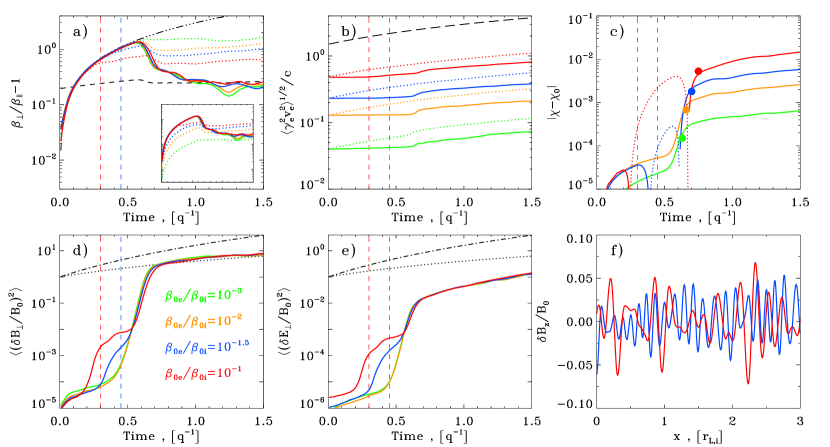
Figure 1.— Temporal and spatial development of compression-driven instabilities, for different choices of the electron-to-ion temperature ratio $T_{0e}/T_{0i}=\beta_{0e}/\beta_{0i}$, as detailed in the legend of panel (d). We fix $\beta_{0i}=20$, $v_{A0i}/c=0.05$, $\omega_{0ci}/q=50$ and $m_{i}/m_{e}=64$. We show the temporal evolution of the following quantities, with $q^{-1}$ as our time unit ($q$ being the compression rate): (a) Ion (solid) and electron (dotted) anisotropy $\beta_{\perp}/\beta_{\parallel}-1$, together with the threshold at marginal stability for the ion cyclotron instability (dashed black line, see Eq. (19)). The triple-dot-dashed black line follows the track expected from compression alone. In the subpanel, the electron anisotropy (dotted lines) is multiplied by $\beta_{0e}^{0.5}$, to emphasize the dependence $A_{e,\rm MS}\propto\beta_{e\parallel}^{-{0.5}}$ at the threshold of marginal stability for the whistler mode. (b) Mean momentum dispersion of electrons, along (solid) or perpendicular (dotted) to the mean field. The dashed black line shows the expected evolution of the transverse component, due to compression alone (i.e., $\propto(1+q\,t)$). (c) Efficiency of electron heating or cooling, as quantified by the $\chi$ parameter defined in Eq. (13) relative to its initial value $\chi_{0}$ (solid if $\chi-\chi_{0}\geq 0$, dotted if $<0$). The filled circles show the predictions of our analytical model at the end of the exponential growth of the ion cyclotron instability (see Section 4). (d) Magnetic energy density in the transverse component $\langle\delta B_{\perp}^{2}\rangle=\langle\delta B_{y}^{2}+\delta B_{z}^{2}\rangle$, in units of $B_{0}^{2}$. For reference, we also plot $(1+q\,t)^{2}$ (dotted black line) and $(1+q\,t)^{4}$ (dot-dashed black line, as expected for the evolution of the mean field energy). (e) Electric energy density in the transverse component $\langle\delta E_{\perp}^{2}\rangle=\langle\delta E_{y}^{2}+\delta E_{z}^{2}\rangle$, in units of $B_{0}^{2}$. The dotted and the dot-dashed black lines are the same as in panel (d), apart from the normalization. Finally, panel (f) presents — at the times indicated with the vertical dashed lines in all the other panels — the spatial profile of $\delta B_{z}/B_{0}$, as a function of the longitudinal coordinate $x$, measured in units of the ion Larmor radius $r_{L,i}$.

5.1. Dependence on the Temperature Ratio

In this section, we illustrate the dependence on the electron-to-ion temperature ratio $T_{0e}/T_{0i}=\beta_{0e}/\beta_{0i}$, for a representative case with $\beta_{0i}=20$, $v_{A0i}/c=0.05$, $\omega_{0ci}/q=50$ and $m_{i}/m_{e}=64$. We vary the electron-to-ion temperature ratio from $\beta_{0e}/\beta_{0i}=10^{-3}$ up to $10^{-1}$.

In the range $T_{0e}/T_{0i}\lesssim 0.1$ explored in LABEL:tratio, the development of the ion cyclotron instability is not sensitive to the electron thermal content. In fact, LABEL:tratio shows that the time of growth of the ion cyclotron instability ($q\,t\simeq 0.6$) and the saturation values of the magnetic and electric energy ($\langle\delta B_{\perp}^{2}\rangle/|\langle\mbox{\boldmath{$B$}}\rangle|^{2}\sim 0.3$ in LABEL:tratio(d) and $\langle\delta E_{\perp}^{2}\rangle/|\langle\mbox{\boldmath{$B$}}\rangle|^{2}\sim 3\times 10^{-3}$ in LABEL:tratio(e), respectively) are all insensitive to the electron-to-ion temperature ratio. Moreover, the secular evolution that follows the exponential phase of the ion cyclotron instability (at $q\,t\gtrsim 0.7$) is the same, regardless of $T_{0e}/T_{0i}$. Once the energy of the ion cyclotron waves reaches $\langle\delta B_{\perp}^{2}\rangle^{1/2}/|\langle\mbox{\boldmath{$B$}}\rangle|\sim 0.1$, efficient pitch-angle scattering brings the ion anisotropy (LABEL:tratio(a)) back to the threshold of marginal stability in Eq. (19) (which is indicated in LABEL:tratio(a) with a dashed black line). At $q\,t\gtrsim 0.9$, the ion anisotropy follows the same track of marginal stability, regardless of the initial electron temperature. In short, the ion physics does not depend on the electron thermal content.

The choice of initial electron temperature can affect the electron physics before the onset of the ion cyclotron instability. For cold electrons ($T_{0e}/T_{0i}=10^{-3}$ in green and $T_{0e}/T_{0i}=10^{-2}$ in orange), the ion cyclotron instability starts to grow when the electron anisotropy has not reached yet the threshold for the electron whistler instability in Eq. (25) (corresponding to $A_{e,\rm MS}\simeq 1.3$ for $T_{0e}/T_{0i}=10^{-2}$ and to $A_{e,\rm MS}\simeq 3.9$ for $T_{0e}/T_{0i}=10^{-3}$). In this case, the electron anisotropy is not strong enough to trigger anisotropy-driven instabilities on electron scales, and no signs of electron physics are present. In particular, the temporal evolution of the magnetic and electric energy (LABEL:tratio(d) and (e), respectively) is the same at all times, regardless of the electron temperature. The only dependence on $T_{0e}/T_{0i}$ in this regime of cold electrons ($T_{0e}/T_{0i}\lesssim 10^{-2}$) appears in the value of electron anisotropy after the growth of the ion cyclotron instability (compare the green and orange dotted lines in LABEL:tratio(a) at $q\,t\gtrsim 0.6$). The degree of electron anisotropy is regulated by the mechanism of electron heating during the ion phase, as we detail below.

At higher electron temperatures ($T_{0e}/T_{0i}=10^{-1.5}$ in blue and $T_{0e}/T_{0i}=10^{-1}$ in red), the threshold for the whistler instability — which corresponds to $A_{e,\rm MS}\simeq 0.7$ for $T_{0e}/T_{0i}=10^{-1.5}$ and to $A_{e,\rm MS}\simeq 0.4$ for $T_{0e}/T_{0i}=10^{-1}$ — is reached before the onset of the ion cyclotron mode. So, the whistler instability can grow, generating transverse electromagnetic waves (see Appendix B in Paper I for further details), and producing a bump at early times ($q\,t\simeq 0.4$) in the magnetic and electric energy of LABEL:tratio(d) and (e), respectively. In Appendix A, we estimate analytically the saturation values of the magnetic and electric energy produced by the whistler instability, as a function of the flow conditions. Our estimates are in good agreement with the results of our simulations, regarding the dependence on both $T_{0e}/T_{0i}$ (investigated in LABEL:tratio) and $m_{i}/m_{e}$ (see LABEL:mimehigh for details).

During the whistler phase at $0.3\lesssim q\,t\lesssim 0.55$, the electron anisotropy remains at the threshold of marginal stability, see the dotted blue and red lines in LABEL:tratio(a). In contrast, the ion anisotropy still follows the track $(1+q\,t)^{2}-1$ expected from compression alone (indicated by the triple-dot-dashed line in LABEL:tratio(a)), suggesting that ions do not participate in the whistler instability. We expect the electron anisotropy during the whistler phase ($0.3\lesssim q\,t\lesssim 0.55$) to scale as $A_{e,\rm MS}\propto\beta_{{e\parallel}}^{-{0.5}}$, as in Eq. (25). Once we multiply the electron anisotropy by a factor of $\beta_{0e}^{{0.5}}$, we find that the temporal tracks for $T_{0e}/T_{0i}=10^{-1.5}$ and $10^{-1}$ almost overlap (blue and red dotted lines in the subpanel of LABEL:tratio(a)), indicating that the condition of marginal stability in Eq. (25) indeed regulates the level of electron anisotropy after the onset of the whistler instability. While it is not suprising that the electron anisotropy stays at the threshold $\sim A_{e,\rm MS}$ during the electron phase at $0.3\lesssim q\,t\lesssim 0.55$, we remark that a similar degree of anisotropy is preserved after the growth of the ion cyclotron instability at $q\,t\gtrsim 0.6$, which justifies our ansatz in Eq. (24) (see the first term in the square brackets).

The electron whistler instability generates transverse electromagnetic waves on electron scales. At marginal stability, the characteristic wavelength and oscillation frequency of the electron whistler mode are respectively (Kennel & Petschek, 1966; Yoon & Davidson, 1987; Yoon et al., 2011; Bashir et al., 2013)

$$\lambda_{e}\simeq\frac{2\pi}{A_{e,\rm MS}^{1/2}}\,\frac{c}{\omega_{\rm pe}}~{}~{}{\rm and}~{}~{}\omega_{e}\simeq\frac{A_{e,\rm MS}}{A_{e,\rm MS}+1}\,\omega_{ce}~{}.$$ (30)

Since we account for the possibility that electrons are ultra-relativistic, the proper definitions of the electron cyclotron frequency and plasma frequency are

$$\omega_{ce}=\frac{e|\langle\mbox{\boldmath{$B$}}\rangle|}{\langle\gamma_{e}\rangle m_{e}c}~{}~{}{\rm and}~{}~{}\omega_{\rm pe}=\sqrt{\frac{4\pi ne^{2}}{\langle\gamma_{e}\rangle m_{e}}}~{}~{}.$$ (31)

In LABEL:tratio(f), we show the spatial pattern of the $\delta B_{z}$ component of whistler waves, measured at the time indicated with the blue and red dashed vertical lines in all the other panels (for $T_{0e}/T_{0i}=10^{-1.5}$ and $10^{-1}$, respectively). In units of the ion Larmor radius $r_{L,i}$, the characteristic wavelength of the whistler instability is

$$\frac{\lambda_{e}}{r_{L,i}}\simeq 2\pi A_{e,\rm MS}^{-1/2}\sqrt{\frac{2\langle\gamma_{e}\rangle m_{e}}{3\,\beta_{0i}\,m_{i}}}~{}~{}~{}.$$ (32)

In LABEL:tratio, we employ $\beta_{0i}=20$ and $m_{i}/m_{e}=64$. For $T_{0e}/T_{0i}=10^{-1.5}$, taking $A_{e,\rm MS}\simeq 1$ from the dotted bue line in LABEL:tratio(a), we expect from Eq. (32) that $\lambda_{e}/r_{L,i}\simeq 0.2$, which is in good agreement with the spatial periodicity of the blue line in LABEL:tratio(f). Similarly, for $T_{0e}/T_{0i}=10^{-1}$, taking $A_{e,\rm MS}\simeq 0.6$ from the dotted red line in LABEL:tratio(a), we expect $\lambda_{e}/r_{L,i}\simeq 0.25$, which agrees with the spatial pattern of the red line in LABEL:tratio(f). We have extensively checked the scalings in Eq. (32), most importantly regarding the dependence on $T_{0e}/T_{0i}$ and $m_{e}/m_{i}$. In the limit of non-relativistic electrons (so, $\langle\gamma_{e}\rangle\simeq 1$), we find from Eq. (32) that $\lambda_{e}/r_{L,i}\propto\beta_{{e\parallel}}^{0.25}$, since $A_{e,\rm MS}\propto\beta_{{e\parallel}}^{-{0.5}}$. This scaling is consistent with the numerical findings of Gary & Karimabadi (2006).

We conclude by discussing the efficiency of electron heating, as a function of the electron-to-ion temperature ratio. In LABEL:tratio(c), we plot the temporal evolution of the $\chi$ parameter defined in Eq. (13) relative to its initial value $\chi_{0}$ (solid lines if $\chi-\chi_{0}\geq 0$, dotted if $<0$). The filled circles in LABEL:tratio show, for different choices of $T_{0e}/T_{0i}$, our analytical prediction for the change in the $\chi$ parameter — as derived from the theory outlined in Section 4 — at the end of the exponential phase of the ion cyclotron instability. Regardless of the initial electron temperature, the growth of the ion cyclotron waves at $q\,t\simeq 0.7$ leads to substantial electron heating, whose magnitude is properly captured by our analytical model (compare the lines with the filled circles of the same color). The increase in the $\chi$ parameter is more pronounced for higher values of $T_{0e}/T_{0i}$. This can be easily understood from the scalings in Eqs. (26)-(28), as we now explain.

At small values of $T_{0e}/T_{0i}$ (green line in LABEL:tratio(c), for $T_{0e}/T_{0i}=10^{-3}$), electron heating by the ion cyclotron instability is dominated by the E-cross-B term in Eq. (28), which is insensitive to the electron temperature. In Paper I, we have demonstrated that the E-cross-B contribution dominates if $\beta_{0e}\lesssim 2\,m_{e}/m_{i}$. In this case, Eq. (28) together with Eq. (29) show that the increase in the $\chi$ parameter is independent of $T_{0e}/T_{0i}$ (as long as $\langle\gamma_{0e}\rangle\simeq 1$), which we have confirmed by running dedicated simulations with even smaller values of the electron-to-ion temperature ratio, $T_{0e}/T_{0i}=2.5\times 10^{-4}$ and $T_{0e}/T_{0i}=10^{-4}$ (not shown in LABEL:tratio).

For $\beta_{0e}\gtrsim 2\,m_{e}/m_{i}$, which corresponds to $T_{0e}/T_{0i}\gtrsim 1.5\times 10^{-3}$ for the parameters adopted in LABEL:tratio, the physics of electron heating is controlled by the terms in Eq. (26) and Eq. (27), with the former that typically dominates, due to its weaker dependence on $\langle\delta B_{\perp}^{2}\rangle/|\langle\mbox{\boldmath{$B$}}\rangle|^{2}\ll 1$. While the E-cross-B term accounts for as much as $64\%$ of the mean electron energy gain for $T_{0e}/T_{0i}=10^{-3}$, its contribution falls down to $15\%$ for $T_{0e}/T_{0i}=10^{-2}$, and it is even smaller for higher values of $T_{0e}/T_{0i}$ (see the rightmost column in Table 1). In parallel, the combination of $\langle\Delta\gamma_{\partial B}\rangle>0$ and $\langle\Delta\gamma_{\rm curv}\rangle<0$ results in a fractional contribution to electron heating that increases from $31\%$ at $T_{0e}/T_{0i}=10^{-3}$ up to $72\%$ at $T_{0e}/T_{0i}=10^{-2}$ and is even larger for higher $T_{0e}/T_{0i}$ (see the leftmost column in Table 1). If the term in Eq. (26) dominates over the contribution in Eq. (27), as it happens for all the values of $T_{0e}/T_{0i}$ investigated in LABEL:tratio (compare the first and second column in Table 1), we expect the electron fractional energy gain to increase initially as $\propto T_{0e}/T_{0i}$, as long as the second term in the square brackets of Eq. (26) is smaller than the first one, and then as $\propto T_{0e}^{0.5}/T_{0i}^{0.5}$. While the former scaling is the same as in the grad-B term of Eq. (27), the latter is shallower, which explains why for high values of $T_{0e}/T_{0i}$ the fractional contribution to electron heating by the grad-B term becomes increasingly larger, at the expense of the term in Eq. (26) (compare first and second columns in Table 1 between $T_{0e}/T_{0i}=10^{-1.5}$ and $10^{-1}$).

Finally, we point out that our model tends to overestimate the actual increase in the $\chi$ parameter observed for high values of $T_{0e}/T_{0i}$ (compare the red line and the filled red circle in LABEL:tratio(c)). As we discuss in Appendix B, this is due to the the early decrease in the $\chi$ parameter that accompanies the growth of electron whistler waves. The value of $\chi-\chi_{0}$ becomes as low as $\simeq-4\times 10^{-3}$ at $q\,t\simeq 0.6$ (dotted red line in LABEL:tratio(c)), so that the subsequent increase driven by the ion cyclotron instability falls short of our analytical prediction, which does not take into account the degree of electron cooling during the whistler phase. Extrapolating this argument to even higher values of the electron-to-ion temperature ratio, one might be tempted to infer an upper limit on $T_{0e}/T_{0i}$, where cooling by the whistler instability balances heating by the ion cyclotron mode. However, the following caveats should be considered.

As we demonstrate in Section 5.4, as $\omega_{0ci}/q$ increases, the ion cyclotron instability appears earlier, and in the astrophysically-relevant limit $\omega_{0ci}/q\gg 1$ it will grow soon after the ion anisotropy exceeds the threshold in Eq. (19). Then, the condition ${0.55}/\beta_{{e\parallel}}^{{0.5}}\lesssim{0.65}/\beta_{{i\parallel}}^{{0.4}}$ required for the whistler instability to have a smaller threshold than the ion cyclotron mode, such that to precede the ion cyclotron growth, can be recast as a lower limit on the electron-to-ion temperature ratio

$$\frac{T_{0e}}{T_{0i}}\gtrsim\frac{0.7}{\beta_{0i}^{0.2}}\sim 0.3-0.5~{}~{}~{},$$ (33)

for the range of $\beta_{0i}\sim 5-30$ expected in accretion flows. This is already in the regime where oblique mirror modes cannot be neglected in the evolution of the system (see Paper I), so one needs to perform 2D simulations. A detailed study of electron heating in the regime $T_{0e}/T_{0i}\gtrsim 0.3$ — which must be performed with 2D simulations having $\omega_{0ci}/q\gg 1$ — will be presented elsewhere.

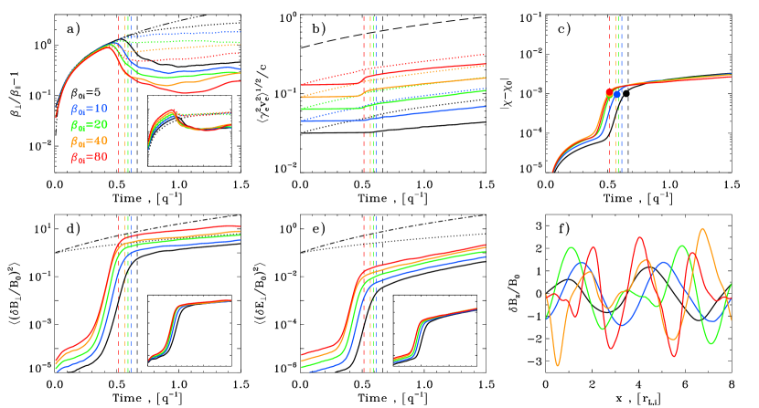
Figure 2.— Temporal and spatial development of compression-driven instabilities, for different choices of the ion plasma beta $\beta_{0i}$, as detailed in the legend of panel (a). We fix $\beta_{0e}/\beta_{0i}=10^{-2}$, $v_{A0i}/c=0.05$, $\omega_{0ci}/q=100$ and $m_{i}/m_{e}=16$. See the caption of LABEL:tratio for details. In the subpanel of LABEL:beta(a), we multiply the anisotropy of both ions and electrons by $\beta_{0i}^{{0.4}}$, showing that this leaves no residual dependence at late times, when the ion anisotropy approaches the threshold of marginal stability in Eq. (19). In the subpanels of LABEL:beta(d) and (e), the magnetic and electric energy densities are multiplied by $\beta_{0i}^{-0.5}$, showing that this leaves no residual dependence (see Appendix A for an analytical justification of this scaling).

Table 1Fractional Contributions to Electron Heating

Run	$\frac{\langle\Delta\gamma_{\partial B}-|\Delta\gamma_{\rm curv}|\rangle}{\langle\Delta\gamma_{e,q}\rangle}$	$\frac{\langle\Delta\gamma_{\nabla B}\rangle}{\langle\Delta\gamma_{e,q}\rangle}$	$\frac{\langle\Delta\gamma_{E\times B}\rangle}{\langle\Delta\gamma_{e,q}\rangle}$
$\beta_{0e}/\beta_{0i}=10^{-3}$	0.31	0.05	0.64
$\beta_{0e}/\beta_{0i}=10^{-2}$	0.72	0.13	0.15
$\beta_{0e}/\beta_{0i}=10^{-1.5}$	0.79	0.15	0.06
$\beta_{0e}/\beta_{0i}=10^{-1}$	0.78	0.19	0.03
Note: We fix $\beta_{0i}=20$, $v_{A0i}/c=0.05$, $\omega_{0ci}/q=50$ and $m_{i}/m_{e}=64$.

5.2. Dependence on the Ion Plasma Beta

In this section, we examine the dependence of our results on the ion plasma beta $\beta_{0i}$, for a representative case with fixed $\beta_{0e}/\beta_{0i}=10^{-2}$, $v_{A0i}/c=0.05$, $\omega_{0ci}/q=100$ and $m_{i}/m_{e}=16$. We explore the range $\beta_{0i}=5-80$, but we argue that our results apply down to $\beta_{0i}\gtrsim 1$.

In LABEL:beta, we show that the level of magnetic and electric energy (panel (d) and (e), respectively) resulting from the ion cyclotron instability increases monotonically with $\beta_{0i}$ (from black to red as $\beta_{0i}$ varies from 5 up to 80). Once normalized to the mean field energy $|\langle\mbox{\boldmath{$B$}}\rangle|^{2}/8\pi$ — whose temporal evolution is shown with a dot-dashed black line in LABEL:beta(d) — we find that for $\beta_{0i}=20$ (green line in LABEL:beta(d)), the magnetic energy in ion cyclotron waves reaches $\langle\delta B_{\perp}^{2}\rangle/|\langle\mbox{\boldmath{$B$}}\rangle|^{2}\sim 0.3$ at the end of the exponential growth of the ion cyclotron mode ($q\,t\simeq 0.6$). Also, both the magnetic and the electric energies scale as $\propto\beta_{0i}^{0.5}$. This result, which is derived analytically in Appendix A, is confirmed in the subpanels of LABEL:beta(d) and (e), where we plot the temporal evolution of the magnetic and electric energy density multiplied by $\beta_{0i}^{-0.5}$. The fact that the different curves overlap demonstrates that

$$\frac{\langle\delta B_{\perp}^{2}\rangle}{|\langle\mbox{\boldmath{$B$}}\rangle|^{2}}\propto\beta_{0i}^{0.5}~{}~{}{\rm and}~{}~{}\frac{\langle\delta E_{\perp}^{2}\rangle}{|\langle\mbox{\boldmath{$B$}}\rangle|^{2}}\propto\beta_{0i}^{0.5}~{},$$ (34)

everything else being fixed. A posteriori, this lends support to our ansatz in Eq. (22) and Eq. (23). Moreover, LABEL:beta(d) shows that our assumption of $\langle\delta B_{\perp}^{2}\rangle/|\langle\mbox{\boldmath{$B$}}\rangle|^{2}\lesssim 1$ — which we have employed in Paper I and in Section 4 — is satisfied in the range of $\beta_{0i}$ investigated in this work.

We remark that both the normalization and the $\beta_{0i}-$dependence of Eq. (22) are in agreement with earlier studies of the compression-driven ion cyclotron instability performed with hybrid codes (e.g., Hellinger & Trávníček, 2005). The scaling $\langle\delta B_{\perp}^{2}\rangle\propto\beta_{0i}^{0.5}$ had previously been found also via hybrid simulations of undriven systems by Gary et al. (1997, 2000). In addition, these studies had assessed the dependence on $\beta_{0i}$ of the ion anisotropy at marginal stability, see Eq. (19). In LABEL:beta(a), we confirm that, due to pitch-angle scattering by the transverse ion cyclotron waves, the ion anisotropy at $q\,t\gtrsim 0.6$ is reduced back to its value at the threshold of marginal stability. In agreement with Eq. (19), the residual degree of anisotropy is smaller for higher $\beta_{0i}$. More precisely, we confirm the scaling $A_{i,\rm MS}\propto\beta_{0i}^{-{0.4}}$ in the subpanel of LABEL:beta(a), where we multiply the different curves by a factor of $\propto\beta_{0i}^{{0.4}}$. The fact that the different solid lines overlap confirms the scaling in Eq. (19) for the ion anisotropy at marginal stability. Interestingly, the subpanel of LABEL:beta(a) shows that the electron anisotropy also scales as $\propto\beta_{0i}^{-{0.4}}$, and it is consistently a factor of $\sim 5$ larger than the ion anisotropy at marginal stability $A_{i,\rm MS}$ (see the dotted lines in the subpanel of LABEL:beta(a), where all the curves have been multiplied by a factor of $\propto\beta_{0i}^{{0.4}}$). This justifies our ansatz in Eq. (24), as a constraint on the degree of electron anisotropy in the absence of the electron whistler phase (see the second term in the square brackets of Eq. (24)).

From the ion anisotropy at marginal stability in Eq. (19), we can write the dominant wavelength of the ion cyclotron mode as $\lambda_{i}\simeq 2\pi\,A_{i,\rm MS}^{-1}\,c/\omega_{\rm pi}$, where we have taken the limit of weak anisotropy $A_{i,\rm MS}\ll 1$ appropriate for $\beta_{0i}\gtrsim 1$ (see Eq. (20)). Since $A_{i,\rm MS}\propto\beta_{{i\parallel}}^{-{0.4}}$, we find that $\lambda_{i}\propto\beta_{{i\parallel}}^{{0.4}}c/\omega_{\rm pi}$, that is remarkably similar to the scaling of the ion Larmor radius: $r_{L,i}\propto\beta_{0i}^{1/2}c/\omega_{\rm pi}$. It follows that the wavelength of the dominant mode should be nearly independent of $\beta_{0i}$, once measured in units of the ion Larmor radius. More precisely, $\lambda_{i}\propto\beta_{0i}^{-0.1}r_{L,i}$. The dependence of the dominant wavelength on $\beta_{0i}$ is shown in LABEL:beta(f), where we plot the spatial pattern of the $\delta B_{z}$ component of the ion cyclotron waves, at the times indicated with the vertical dashed lines in the other panels. We confirm that the dominant wavelength is nearly the same, in units of the ion Larmor radius, with a residual tendency for shorter wavelengths at higher $\beta_{0i}$, in agreement with the expected scaling $\lambda_{i}\propto\beta_{0i}^{-0.1}r_{L,i}$. Similarly, we have verified that the oscillation period of the ion cyclotron waves agrees with Eq. (21).

Regarding electron heating by the ion cyclotron instability, LABEL:beta(c) shows that the increase in the $\chi$ parameter is nearly independent of $\beta_{0i}$. This might appear surprising, given the strong dependence on $\beta_{0i}$ of the $\langle\Delta\gamma_{\nabla B}\rangle$ and $\langle\Delta\gamma_{E\times B}\rangle$ terms in Eq. (27) and Eq. (28), respectively. However, for the parameters employed in LABEL:beta, we find that if $\beta_{0i}\gtrsim 20$ the combination $\langle\Delta\gamma_{\partial B}-|\Delta\gamma_{\rm curv}|\rangle$ in Eq. (26) dominates the process of electron heating (see the first column in Table 2). Since the dependence of Eq. (26) on $\beta_{0i}$ is extremely weak ($\propto\beta_{0i}^{0.1}$, in the regime relevant for LABEL:beta), it is not surprising that the heating efficiency is independent of the ion plasma beta, at $\beta_{0i}\gtrsim 20$. At smaller $\beta_{0i}$, the fractional contribution of the term in Eq. (26) gets smaller, in favor of the E-cross-B term in Eq. (28) (compare the first and the last columns in Table 2). Despite the change in the dominant heating channel, the efficiency of electron heating stays remarkably constant even for $\beta_{0i}\lesssim 20$, both based on our analytical model (filled circles in LABEL:beta(c)) and confirmed by our simulations (solid lines in LABEL:beta(c)). Yet, at $\beta_{0i}\lesssim 20$, this apparent independence of the heating efficiency on the ion plasma beta should be regarded as a mere coincidence. At even smaller values of $\beta_{0i}$, we expect the beta-dependence of the E-cross-B term in Eq. (28) to become apparent.

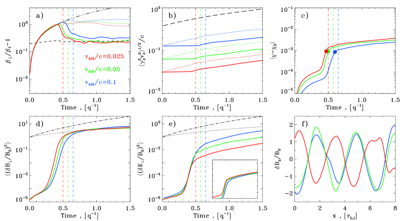
Figure 3.— Temporal and spatial development of compression-driven instabilities, for different choices of the Alfvén velocity $v_{A0i}/c$, as detailed in the legend of panel (a). We fix $\beta_{0i}=20$, $\beta_{0e}/\beta_{0i}=10^{-2}$, $\omega_{0ci}/q=100$ and $m_{i}/m_{e}=16$. See the caption of LABEL:tratio for details. In the subpanel of LABEL:beta(e), the electric energy density is multiplied by $v_{A0i}^{-2}$, showing that this leaves no residual dependence (see Appendix A for an analytical justification of this scaling).

Table 2Fractional Contributions to Electron Heating

Run	$\frac{\langle\Delta\gamma_{\partial B}-|\Delta\gamma_{\rm curv}|\rangle}{\langle\Delta\gamma_{e,q}\rangle}$	$\frac{\langle\Delta\gamma_{\nabla B}\rangle}{\langle\Delta\gamma_{e,q}\rangle}$	$\frac{\langle\Delta\gamma_{E\times B}\rangle}{\langle\Delta\gamma_{e,q}\rangle}$
$\beta_{0i}=5$	0.30	0.02	0.68
$\beta_{0i}=10$	0.40	0.04	0.56
$\beta_{0i}=20$	0.49	0.09	0.42
$\beta_{0i}=40$	0.56	0.15	0.29
$\beta_{0i}=80$	0.56	0.26	0.18
Note: We fix $\beta_{0e}/\beta_{0i}=10^{-2}$, $v_{A0i}/c=0.05$, $\omega_{0ci}/q=100$ and $m_{i}/m_{e}=16$.

5.3. Dependence on the Alfvén Velocity

In LABEL:sigma we investigate the dependence on the Alfvén velocity, for a representative case with fixed $\beta_{0i}=20$, $\beta_{0e}/\beta_{0i}=10^{-2}$, $\omega_{0ci}/q=100$ and $m_{i}/m_{e}=16$. We explore the range $v_{A0i}/c=0.025-0.1$.

As shown in LABEL:sigma, the temporal evolution of the magnetic energy of ion cyclotron waves (panel (d)) is nearly insensitive to the Alfvén velocity, in agreement with Eq. (22) and Appendix A. The wavelength of the ion cyclotron mode in panel (f) does not explicitly depend on $v_{A0i}/c$, at fixed $\beta_{0i}$ (see Eq. (20) combined with Eq. (19)). In addition, the temporal evolution of the ion anisotropy in LABEL:sigma(a) (solid lines) is nearly independent of $v_{A0i}/c$, in the regime of non-relativistic ions (i.e., with the marginal exception of the case $v_{A0i}/c=0.1$, where the ions are trans-relativistic). The electron anisotropy during the growth of the ion cyclotron mode is $\sim 5\,A_{i,\rm MS}$ (dotted lines in LABEL:sigma(a)), regardless of the Alfvén velocity, which is consistent with our ansatz in Eq. (24) (see the second term in the square brackets).

The only quantity that depends explicitly on the Alfvén velocity is the electric energy density in LABEL:sigma(e), which is expected on analytical grounds to scale as $\propto v_{A0i}^{2}$ (see Appendix A). We confirm this scaling in the subpanel of LABEL:sigma(e), where we multiply the different curves by $v_{A0i}^{-2}$, showing that such rescaling leaves no residual dependence on the Alfvén velocity. Our findings justify the dependence of Eq. (23) on the Alfvén speed.

Finally, from Eqs. (26)-(28), we see that the electron energy change associated with the growth of the ion cyclotron mode has no explicit dependence on the Alfvén velocity, as confirmed in LABEL:sigma(c). The same holds for the increase in the $\chi$ parameter in Eq. (29). However, we point out that this conclusion only applies to the case of non-relativistic electrons, i.e., $\langle\gamma_{0e}\rangle\simeq 1$. If the electrons are ultra-relativistic, at fixed $\beta_{0e}$ and $m_{e}/m_{i}$ we will have that $\langle\gamma_{0e}\rangle\propto v_{A0i}^{2}$, so the electron heating efficiency as quantified by the $\chi$ parameter will increase as $\propto v_{A0i}^{2}$. Albeit not shown in LABEL:sigma, we have verified this scaling in our simulations, in the parameter regime where electrons become ultra-relativistic.

Table 3Fractional Contributions to Electron Heating

Run	$\frac{\langle\Delta\gamma_{\partial B}-|\Delta\gamma_{\rm curv}|\rangle}{\langle\Delta\gamma_{e,q}\rangle}$	$\frac{\langle\Delta\gamma_{\nabla B}\rangle}{\langle\Delta\gamma_{e,q}\rangle}$	$\frac{\langle\Delta\gamma_{E\times B}\rangle}{\langle\Delta\gamma_{e,q}\rangle}$
$v_{A0i}/c=0.025$	0.49	0.09	0.42
$v_{A0i}/c=0.05$	0.49	0.09	0.42
$v_{A0i}/c=0.1$	0.49	0.09	0.42
Note: We fix $\beta_{0i}=20$, $\beta_{0e}/\beta_{0i}=10^{-2}$, $\omega_{0ci}/q=100$ and $m_{i}/m_{e}=16$.

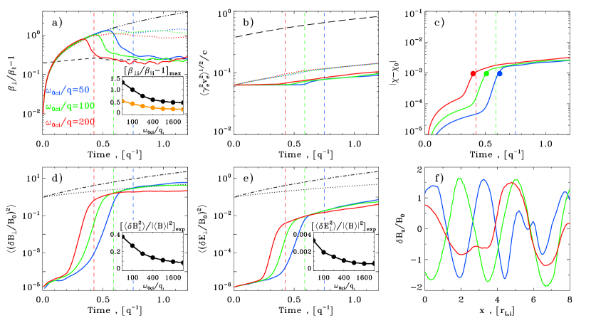
Figure 4.— Temporal and spatial development of compression-driven instabilities, for different choices of the parameter $\omega_{0ci}/q$. We fix $\beta_{0i}=20$, $\beta_{0e}/\beta_{0i}=10^{-2}$, $v_{A0i}/c=0.05$ and $m_{i}/m_{e}=16$, as detailed in the legend of panel (a). In the main plot, we examine the cases $\omega_{0ci}/q=50$ (blue lines), $\omega_{0ci}/q=100$ (green lines) and $\omega_{0ci}/q=200$ (red lines). In the subpanels of LABEL:mag(a), (d) and (e) we extend our study to $\omega_{0ci}/q=3200$. In the subpanel of LABEL:mag(a), we show both the peak value of the ion anisotropy (filled black circles) and the time at which the ion anisotropy peaks (filled orange circles). In the subpanels of LABEL:mag(d) and (e), we show respectively the magnetic and electric energies in ion cyclotron waves normalized to the mean field energy, measured at the end of the exponential phase of the ion cyclotron growth. We remark that the horizontal axis in the subpanels of LABEL:mag(a), (d) and (e) shows the ratio $\omega_{0ci}/q$ on a logarithmic scale, from $\omega_{0ci}/q=50$ up to 3200 (with each tick mark corresponding to an increase by a factor of two). See LABEL:tratio for details.

5.4. Dependence on the Compression Rate

In this section, we analyze the dependence of our results on the compression rate, or more specifically on the ratio $\omega_{0ci}/q$, which is much larger than unity in astrophysical accretion flows. We focus on a representative case with fixed $\beta_{0i}=20$, $\beta_{0e}/\beta_{0i}=10^{-2}$, $v_{A0i}/c=0.05$ and $m_{i}/m_{e}=16$. We find that only for $\omega_{0ci}/q\lesssim 200$ we can capture the physics of both ions and electrons with sufficient accuracy, and in LABEL:mag we show the cases $\omega_{0ci}/q=50$ (blue lines), $\omega_{0ci}/q=100$ (green) and $\omega_{0ci}/q=200$ (red). Yet, if we are only interested in the ion physics, we can extend our investigation to much larger values of $\omega_{0ci}/q$. This is shown in the subpanels of LABEL:mag(a), (d) and (e), where we study the development of the ion cyclotron instability up to the case $\omega_{0ci}/q=3200$, comparable to the range $\omega_{0ci}/q=1000-4000$ explored in the hybrid simulations by Hellinger & Trávníček (2005).

As shown in LABEL:mag, the development of the ion cyclotron instability is similar, for different values of $\omega_{0ci}/q$. In all cases, the magnetic and electric energies grow exponentially (panels (d) and (e), respectively), with a growth rate that scales with the compression rate, rather than with the ion cyclotron frequency (see also Riquelme et al., 2014, for similar conclusions in a system dominated by the mirror instability). The wavelength of the dominant mode is nearly insensitive to $\omega_{0ci}/q$, as shown in LABEL:mag(f), with only a marginal tendency for longer wavelengths at higher $\omega_{0ci}/q$. On the other hand, the growth of the unstable modes happens earlier for higher values of $\omega_{0ci}/q$. This trend is also apparent in LABEL:mag(a), where we show the ion anisotropy with solid lines. For faster compressions (i.e., smaller $\omega_{0ci}/q$, blue line), the system goes farther into the unstable region, before pitch-angle scattering off the growing ion cyclotron waves brings the ion anisotropy back to the threshold of marginal stability (shown with a black dashed line in LABEL:mag(a)). Since the anisotropy overshoot into the unstable region is more pronounced for smaller $\omega_{0ci}/q$, stronger magnetic fluctuations are needed to drive the system back to marginal stability, at smaller $\omega_{0ci}/q$ (see the magnetic energy at the end of the exponential phase in LABEL:mag(d)). In contrast, for slow compressions (red line in LABEL:mag(a)), the ion anisotropy does not move far from the threshold condition (see also Riquelme et al., 2014, for similar conclusions in a system dominated by the mirror instability), and the amplitude of the ion cyclotron waves at the end of the exponential phase tends to be smaller (compare red and blue lines in LABEL:mag(d)).

In the subpanels of LABEL:mag(a), (d) and (e) we extend our analysis to larger values of $\omega_{0ci}/q$, towards the astrophysically-relevant limit $\omega_{0ci}/q\gg 1$. In these three subpanels, we plot on the horizontal axis the value of $\omega_{0ci}/q$ in the range from $50$ to $3200$, with each tick mark corresponding to an increment by a factor of two (so, logarithmic scale). In the subpanel of LABEL:mag(a), we show both the peak value of the ion anisotropy (filled black circles) and the time at which the ion anisotropy peaks (filled orange circles), which is a good proxy for the onset time of the ion cyclotron instability. In the subpanels of LABEL:mag(d) and (e), we show respectively the magnetic and electric energies in ion cyclotron waves normalized to the mean field energy, measured at the end of the exponential phase of the ion cyclotron instability.

From the subpanel in LABEL:mag(a), we argue that both the onset time of the instability and the maximum ion anisotropy approach a constant value in the limit $\omega_{0ci}/q\gg 1$, with no residual dependence on this parameter. More precisely, the onset time of the ion cyclotron waves, which is $\simeq 0.4\,q^{-1}$ for $\omega_{0ci}/q=100$, tends toward $0.25\,q^{-1}$ for $\omega_{0ci}/q\gg 1$. Similarly, for the parameters adopted in LABEL:mag, the peak ion anisotropy approaches an asymptotic value of $\simeq 0.5$, a factor of two smaller than in our reference case $\omega_{0ci}/q=100$. On the other hand, LABEL:mag(a) demonstrates that at late times the ion anisotropy approaches the same threshold of marginal stability in Eq. (19), regardless of $\omega_{0ci}/q$. For this reason, we argue that, in the absence of the electron whistler phase, the electron anisotropy during the growth of the ion cyclotron instability can still be scaled to the ion anisotropy at marginal stability $A_{i,\rm MS}$, as assumed in the last term of Eq. (24), but the coefficient of proportionality in the limit $\omega_{0ci}/q\gg 1$ should be a factor of two smaller than in Eq. (24). The trend for a lower degree of electron anisotropy as $\omega_{0ci}/q$ increases is confirmed by the dotted lines of LABEL:mag(a) at $q\,t\gtrsim 0.6$.

With increasing $\omega_{0ci}/q$, the magnetic and electric energies in ion cyclotron waves also approach a constant value, as shown in the subpanels of LABEL:mag(d) and (e), respectively. The value of $\langle\delta B_{\perp}^{2}\rangle/|\langle\mbox{\boldmath{$B$}}\rangle|^{2}$ at the end of the exponential phase of ion cyclotron growth asymptotes to $\simeq 0.1$, roughly a factor of three smaller than in our standard case $\omega_{0ci}/q=100$ (subpanel in LABEL:mag(d)). The asymptotic value of $\langle\delta E_{\perp}^{2}\rangle/|\langle\mbox{\boldmath{$B$}}\rangle|^{2}$ is smaller than for $\omega_{0ci}/q=100$ by a similar factor (subpanel in LABEL:mag(e)). In summary, we conclude that the coefficient in Eq. (22) should be reduced by a factor of three, for $\omega_{0ci}/q\gg 1$.

In our analytical model of electron heating, based on Eqs. (22)-(24) and Eqs. (26)-(28), we have not taken into account the explicit dependence on $\omega_{0ci}/q$, which would change the coefficients in Eq. (22) and Eq. (24) in the way we have just described. This explains why our model of electron heating, which is benchmarked at $\omega_{0ci}/q=100$ (green line in LABEL:mag(c)), tends to overpredict the heating efficiency at higher values of $\omega_{0ci}/q$ (red line for $\omega_{0ci}/q=200$), whereas it underpredicts the results of our simulations at lower $\omega_{0ci}/q$ (blue line for $\omega_{0ci}/q=50$).

Table 4Fractional Contributions to Electron Heating

Run	$\frac{\langle\Delta\gamma_{\partial B}-|\Delta\gamma_{\rm curv}|\rangle}{\langle\Delta\gamma_{e,q}\rangle}$	$\frac{\langle\Delta\gamma_{\nabla B}\rangle}{\langle\Delta\gamma_{e,q}\rangle}$	$\frac{\langle\Delta\gamma_{E\times B}\rangle}{\langle\Delta\gamma_{e,q}\rangle}$
$\omega_{0ci}/q=50$	0.49	0.09	0.42
$\omega_{0ci}/q=100$	0.49	0.09	0.42
$\omega_{0ci}/q=200$	0.49	0.09	0.42
Note: We fix $\beta_{0i}=20$, $\beta_{0e}/\beta_{0i}=10^{-2}$, $v_{A0i}/c=0.05$ and $m_{i}/m_{e}=16$.

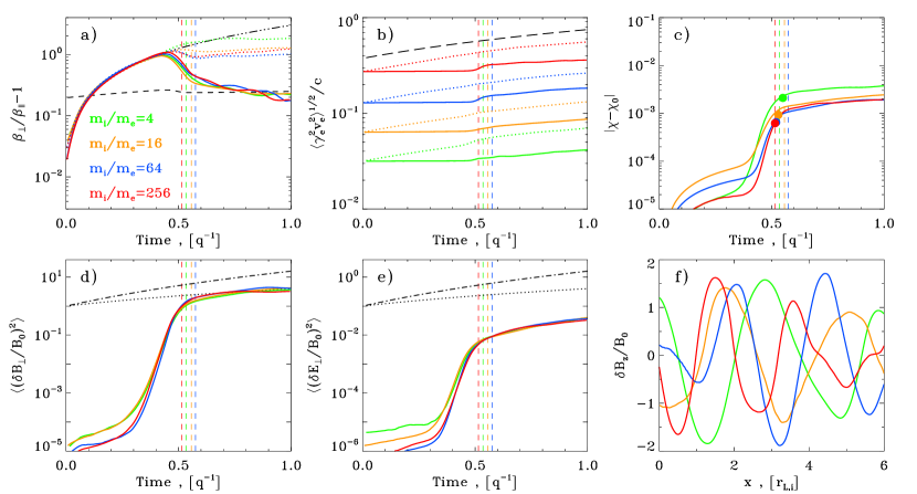
Figure 5.— Temporal and spatial development of compression-driven instabilities, for $T_{0e}/T_{0i}=10^{-2}$ and different choices of the mass ratio $m_{i}/m_{e}$, as detailed in the legend of panel (a). We fix $\beta_{0i}=20$, $v_{A0i}/c=0.05$ and $\omega_{0ci}/q=100$. See the caption of LABEL:tratio for details.

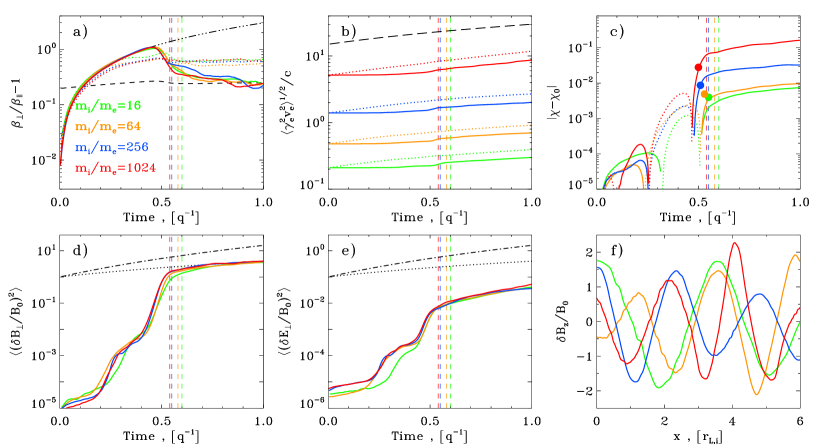
Figure 6.— Temporal and spatial development of compression-driven instabilities, for $T_{0e}/T_{0i}=10^{-1}$ and different choices of the mass ratio $m_{i}/m_{e}$, as detailed in the legend of panel (a). We fix $\beta_{0i}=20$, $v_{A0i}/c=0.05$ and $\omega_{0ci}/q=100$. See the caption of LABEL:tratio for details.

5.5. Dependence on the Mass Ratio

In this section, we investigate the dependence of our results on the mass ratio $m_{i}/m_{e}$, for two representative cases of the electron-to-ion temperature ratio, $T_{0e}/T_{0i}=10^{-2}$ in LABEL:mimelow and $T_{0e}/T_{0i}=10^{-1}$ in LABEL:mimehigh. In both cases, we fix $\beta_{0i}=20$, $v_{A0i}/c=0.05$ and $\omega_{0ci}/q=100$.

For both $T_{0e}/T_{0i}=10^{-2}$ in LABEL:mimelow and $T_{0e}/T_{0i}=10^{-1}$ in LABEL:mimehigh, the development of the ion cyclotron instability does not depend on the mass ratio (see also Riquelme et al., 2014, for similar conclusions in a system dominated by the mirror instability). The curves that describe the evolution of the magnetic and electric energy densities in ion cyclotron waves nearly overlap at $q\,t\gtrsim 0.4$ (panels (d) and (e), respectively), which suggests that the electron physics does not directly affect the growth of the ion cyclotron instability. Similarly, the dominant wavelength of ion cyclotron modes, normalized to the ion Larmor radius as in panel (f), does not depend on the mass ratio. On the other hand, the choice of mass ratio has an influence on the electron anisotropy (dotted lines in panel (a)) and on the efficiency of electron heating (panel (c)), as we now explain in detail.

For $T_{0e}/T_{0i}=10^{-2}$ in LABEL:mimelow, we find that the electron heating efficiency — as quantified by the parameter $\chi$ in LABEL:mimelow(c) — drops as the mass ratio increases from $m_{i}/m_{e}=4$ (green line) to $m_{i}/m_{e}=16$ (orange line), and it remains constant for higher mass ratios (blue for $m_{i}/m_{e}=64$ and red for $m_{i}/m_{e}=256$). This trend corresponds to a change in the dominant mechanism of electron heating. For mass ratios as small as $m_{i}/m_{e}=4$, most of the electron heating comes from the E-cross-B term in Eq. (28) (see the first row in Table 5). This term depends on the mass ratio as $\propto m_{e}/m_{i}$ (see Eq. (28)), so it gives poorer heating efficiencies for higher mass ratios, which explains the trend in LABEL:mimelow(c). On the other hand, if $m_{i}/m_{e}=16$ or higher, the physics of electron heating is primarily controlled by the combination of Eq. (26) and Eq. (27) (see Table 5), which are both independent of $m_{i}/m_{e}$. In turn, this explains why the heating efficiency is independent of mass ratio, for $m_{i}/m_{e}\geq 16$.

In all cases, the results of our simulations (solid lines in LABEL:mimelow(c)) are in excellent agreement with the predictions of our analytic model (filled circles in LABEL:mimelow(c)). The electron anisotropy in LABEL:mimelow(a) (dotted lines) provides support for one of the fundamental assumptions in our model, Eq. (24). In fact, we confirm that in all the cases where electron heating is controlled by terms that depend on the electron thermal content (i.e., Eqs. (26) and (27)), the electron anisotropy during the growth of the ion cyclotron instability stays at $\sim 5\,A_{i,\rm MS}$ independently of the mass ratio. It follows that Eq. (24) can be confidently employed in Eq. (16) to obtain Eq. (26). In LABEL:mimelow(a), the only case that departs from this prediction is $m_{i}/m_{e}=4$ (dotted green line), where indeed the electron heating process is different, being dominated by the E-cross-B term (see the first row in Table 5).

For a higher electron-to-ion temperature ratio ($T_{0e}/T_{0i}=10^{-1}$ in LABEL:mimehigh), the growth of the ion cyclotron mode at $q\,t\simeq 0.5$ follows a phase dominated by electron whistler waves (see the minor bump at $q\,t\simeq 0.3$ in the magnetic and electric energy of panels (d) and (e), respectively). In this case, the electron anisotropy (dotted lines in LABEL:mimehigh(a)) stays at the threshold of marginal stability $A_{e,\rm MS}$ of the electron whistler mode, see Eq. (25). This justifies our ansatz in Eq. (24), in the case $A_{e,\rm MS}\leq 5\,A_{i,\rm MS}$. Pitch-angle scattering off whistler waves constrains the electron anisotropy both at $0.3\lesssim q\,t\lesssim 0.5$, during the whistler phase, and also at $q\,t\gtrsim 0.5$, after the growth of the ion cyclotron instability. In fact, the minor wiggles superimposed over the ion cyclotron waves in LABEL:mimehigh(f) (e.g., see the orange line at $x/r_{L,i}\lesssim 2$) demonstrate that the whistler instability continues to operate at late times, on top of the dominant ion cyclotron mode.

As regard to electron heating for $T_{0e}/T_{0i}=10^{-1}$ (see LABEL:mimehigh(c)), we find that the heating efficiency, as quantified by the $\chi$ parameter, is a monotonic function of $m_{i}/m_{e}$. Here, the physics of electron heating is dominated by the terms in Eqs. (26) and (27). In fact, Table 6 shows that the contribution of the E-cross-B term is always less than $10\%$, for the parameters explored in LABEL:mimehigh. Eqs. (26) and (27) do not explicitly depend on the mass ratio. Yet, at fixed $T_{0e}/T_{0i}$, the mean electron Lorentz factor $\langle\gamma_{0e}\rangle$ that appears in the increase of the $\chi$ parameter (Eq. (29)) will scale with mass ratio as $\langle\gamma_{0e}\rangle\propto m_{i}/m_{e}$, as soon as the electrons become ultra-relativistic. This explains why the increase in the $\chi$ parameter for the cases $m_{i}/m_{e}=16$ and $64$ is nearly identical (green and orange solid lines in LABEL:mimehigh(c), respectively), since the electrons are still non-relativistic. For $m_{i}/m_{e}=256$ and $1024$, the electrons are ultra-relativistic, and the change in the $\chi$ parameter scales as $\Delta\chi\propto\langle\gamma_{0e}\rangle\propto m_{i}/m_{e}$.

Finally, we point out that our model tends to overestimate the actual increase in the $\chi$ parameter for $m_{i}/m_{e}=16$ and 64 (compare the green and orange lines with the corresponding filled circles in LABEL:mimehigh(c)). As we discuss in Appendix B, this is due to the energy lost by electrons to drive the growth of electron whistler waves. The value of $\chi-\chi_{0}$ becomes negative (dotted lines in LABEL:mimehigh(c)), so that the subsequent increase driven by the ion cyclotron instability falls short of our analytical prediction (which does not take into account the degree of electron cooling during the whistler phase). A similar effect has been discussed in Section 5.1.

Table 5Fractional Contributions to Electron Heating

Run	$\frac{\langle\Delta\gamma_{\partial B}-|\Delta\gamma_{\rm curv}|\rangle}{\langle\Delta\gamma_{e,q}\rangle}$	$\frac{\langle\Delta\gamma_{\nabla B}\rangle}{\langle\Delta\gamma_{e,q}\rangle}$	$\frac{\langle\Delta\gamma_{E\times B}\rangle}{\langle\Delta\gamma_{e,q}\rangle}$
$m_{i}/m_{e}=4$	0.22	0.04	0.74
$m_{i}/m_{e}=16$	0.49	0.09	0.42
$m_{i}/m_{e}=64$	0.72	0.13	0.15
$m_{i}/m_{e}=256$	0.81	0.14	0.05
Note: We fix $\beta_{0i}=20$, $\beta_{0e}/\beta_{0i}=10^{-2}$, $v_{A0i}/c=0.05$ and $\omega_{0ci}/q=100$.

Table 6Fractional Contributions to Electron Heating

Run	$\frac{\langle\Delta\gamma_{\partial B}-|\Delta\gamma_{\rm curv}|\rangle}{\langle\Delta\gamma_{e,q}\rangle}$	$\frac{\langle\Delta\gamma_{\nabla B}\rangle}{\langle\Delta\gamma_{e,q}\rangle}$	$\frac{\langle\Delta\gamma_{E\times B}\rangle}{\langle\Delta\gamma_{e,q}\rangle}$
$m_{i}/m_{e}=16$	0.71	0.19	0.10
$m_{i}/m_{e}=64$	0.76	0.21	0.03
$m_{i}/m_{e}=256$	0.78	0.22	$<0.01$
$m_{i}/m_{e}=1024$	0.78	0.22	$<0.01$
Note: We fix $\beta_{0i}=20$, $\beta_{0e}/\beta_{0i}=10^{-1}$, $v_{A0i}/c=0.05$ and $\omega_{0ci}/q=100$.

6. Summary and Discussion

In this work, the second of a series, we have investigated by means of PIC simulations how the efficiency of electron heating by ion velocity-space instabilities (more specifically, the ion cyclotron instability) depends on the physical conditions in low-luminosity two-temperature accretion flows. Pressure anisotropies are continuously generated in collisionless accretion flows due to the fluctuating magnetic fields associated with the non-linear stages of the magnetorotational instability (MRI, Balbus & Hawley 1991, 1998). Field amplifications induced by the MRI, coupled to the adiabatic invariance of the magnetic moments of charged particles, drive a temperature anisotropy $P_{\perp}>P_{\parallel}$ (relative to the local field), which relaxes via velocity-space instabilities.

In Paper I, we have developed a fully-kinetic method for studying velocity-space instabilities in a system where the field is continuously amplified. So, the anisotropy is constantly driven (as a result of the field amplification), rather than assumed as a prescribed initial condition, as in most earlier works. In our setup, the increase in magnetic field is driven by compression, but our results hold regardless of what drives the field amplification, so they can be equally applied to the case where velocity-space instabilities are induced by incompressible shear motions (as in Riquelme et al., 2014).

In Paper I we found that, for the values of ion plasma beta $\beta_{0i}\sim 5-30$ expected in the midplane of low-luminosity accretion flows (e.g., Sa̧dowski et al., 2013), the dominant mode for $T_{0e}/T_{0i}\lesssim 0.2$ is the ion cyclotron instability, rather than the mirror instability. Since the wavevector of the ion cyclotron instability is aligned with the mean magnetic field, the relevant physics can be conveniently studied by means of 1D simulations, with the box aligned with the ordered field. In this work, we have studied with 1D PIC simulations the efficiency of electron heating by the ion cyclotron instability. Fully-kinetic simulations with mobile ions and a realistic mass ratio are required to capture at the same time electron-scale and ion-scale instabilities (in our setup, the electron whistler and ion cyclotron modes), as well as to properly describe the energy transfer from ions to electrons.

We have assessed the dependence of the electron heating efficiency on the initial ratio between electron and proton temperatures $T_{0e}/T_{0i}$, on the ion beta $\beta_{0i}$ (namely, the ratio of ion thermal pressure to magnetic pressure), on the Alfvén speed $v_{Ai0}$, on the compression rate $q$ (in units of the proton cyclotron frequency $\omega_{0ci}$), and on the proton to electron mass ratio $m_{i}/m_{e}$, which we have explored up to realistic values. Our analysis does consistently allow for relativistic temperatures and thus it is possible to study the limit of non-relativistic ions and ultra-relativistic electrons that is of particular interest for two-temperature disk models.

Eqs. (26)-(28) emphasize how the various contributions to electron heating — whose physical origin has been described in Paper I — depend on flow conditions. Their sum gives the overall electron energy gain associated with the development of the ion cyclotron instability, and it represents the main result of this paper. Eqs. (26)-(28) show the explicit dependence of the electron energy gain on $T_{0e}/T_{0i}$, $\beta_{0e}$, $\beta_{0i}$ and $m_{i}/m_{e}$, as based on the analytical model presented in Paper I and on the scalings in Eqs. (22)-(24), that we have justified analytically (see Appendix A) and extensively validated with PIC simulations in this work. In addition, we find that our results do not explicitly depend on the Alfvén velocity $v_{A0i}$, as long as it is non-relativistic, and are weakly dependent on $\omega_{0ci}/q$, as long as $\omega_{0ci}/q\gg 1$ ($\omega_{0ci}/q\sim 10^{7}$ in accretion flows, assuming that the timescale of turbulent eddies is comparable to the orbital time). The same weak dependence on $\omega_{0ci}/q\gg 1$ has been found in the shear-driven PIC simulations of velocity-space instabilities in electron-positron plasmas of Riquelme et al. (2014), as regard to the mirror instability.

Another important result of our work concerns the ion response to the ion cyclotron instability. We have assessed that, in our case of driven ion cyclotron instability, the magnetic energy in ion cyclotron waves in the saturated stage scales with the ion beta as $\langle\delta B_{\perp}^{2}\rangle/|\langle\mbox{\boldmath{$B$}}\rangle|^{2}\sim 0.07\,\beta_{0i}^{0.5}$. Pitch-angle scattering off the ion cyclotron waves maintains the ion anisotropy at the threshold of marginal stability $[\beta_{i\perp}/\beta_{i\parallel}-1]_{\rm MS}\simeq{0.65}/\beta_{i\parallel}^{0.4}$. Similarly, in the cases when the electron anisotropy exceeds the threshold for the electron whistler instability before the onset of the ion cyclotron mode, the electron anisotropy is constrained to follow the track of marginal stability $[\beta_{e\perp}/\beta_{e\parallel}-1]_{\rm MS}\simeq{0.55}/\beta_{e\parallel}^{0.5}$ by efficient pitch-angle scattering off the electron whistler waves. These scalings had been widely investigated in the context of undriven velocity-space instabilities (i.e., where the anisotropy is prescribed as an initial condition, see Gary (1993) for a review), yet never with fully-kinetic simulations having mobile ions and a realistic mass ratio, as we employ in this work. In this work, we have estimated such scalings in the case that the ion cyclotron instability is induced by a continuous field amplification.

Our work has implications for the electron physics in two-temperature accretion flows. The electron energy gain associated with the growth of the ion cyclotron instability (see Eqs. (26)-(28)) can be incorporated in GRMHD simulations of low-luminosity accretion flows, by adding a source term to the electron thermal evolution. When coupled to cooling by radiation, this will provide a physically-grounded model for assessing the two-temperature nature of low-luminosity accretion flows like Sgr A^∗ (e.g., Yuan & Narayan, 2014). In this sense, our results provide solid evidence that the ion cyclotron instability has a tendency to equilibrate the ion and electron temperatures, in the regime $T_{0e}/T_{0i}\lesssim 0.2$ where the ion cyclotron instability dominates over the mirror mode.

The physics of electron heating at higher electron-to-ion temperature ratios (i.e., $T_{0e}/T_{0i}\gtrsim 0.2$) is beyond the scope of this work. In this regime, 2D simulations would be needed to assess the efficiency of electron heating by the mirror instability, whose wavevector is oblique with respect to the mean field. On the other hand, at such high electron temperatures ($T_{0e}/T_{0i}\gtrsim 0.3$), the threshold for the electron whistler instability is exceeded before the onset of the mirror mode, for the range of $\beta_{0i}$ expected in accretion flows. As we have found in this work, the growing electron whistler waves will remove thermal energy from the electron population, resulting in net cooling. The relative role of electron cooling by the whistler instability and electron heating by the mirror mode at $T_{0e}/T_{0i}\gtrsim 0.2$ should be investigated with 2D simulations having $\omega_{0ci}/q\gg 1$, and it is deferred to a future work. It will be needed to complement the findings of this paper, which apply to $T_{0e}/T_{0i}\lesssim 0.2$.

Another important question that we have not addressed in this work is the generation of non-thermal electrons, whose emission is required for modeling the broad-band signature of Sgr A^∗ (Yuan et al., 2003; Yuan & Narayan, 2014; Lynn et al., 2014). Particle acceleration due to the development of anisotropy-driven instabilities is generally believed to be quite inefficient (e.g., Kennel & Petschek, 1966), whereas other mechanisms — most notably, magnetic reconnection — might be more promising. PIC simulations of carefully designed systems will be needed to investigate the origin of non-thermal electrons in low-luminosity accretion flows.

Appendix A A. The Electromagnetic Fields at Saturation

In this appendix, we assess how the saturation amplitude of the electromagnetic fields (i.e., at the end of the phase of exponential growth) depends on flow conditions, for both the ion cyclotron instability and the electron whistler instability. As we show below, the physics of field saturation is different in our setup, where the anisotropy is constantly driven, with respect to the case of undriven systems explored by, e.g., Gary et al. (1993); Gary & Winske (1993). Our goal is only to provide approximate scalings, and we refer to, e.g., Gary & Feldman (1978) or Gary & Tokar (1985) (see also Hamasaki & Krall 1973; Yoon 1992; Hellinger et al. 2009, 2013) for a detailed analysis of the evolution of the electromagnetic fields beyond the exponential phase.

At the end of the exponential phase, the magnitude of the magnetic fields has to be large enough such that efficient pitch-angle scattering drives the particle anisotropy back to marginal stability. In other words, the scattering frequency $\nu_{\rm scatt}$ in the fields of the unstable modes will be counter-acting the overall effect of field amplification, which feeds the anisotropy. Following Braginskii (1965) (see also Schekochihin et al. 2008; Rosin et al. 2011; Kunz et al. 2014), it is required that

$$\nu_{\rm scatt}\sim\frac{1}{\beta_{\perp}/\beta_{\parallel}-1}\frac{{\rm d}\ln|\langle\mbox{\boldmath{$B$}}\rangle|}{{\rm d}t}~{}~{}~{},$$ (A1)

where $|\langle\mbox{\boldmath{$B$}}\rangle|\propto(1+q\,t)^{2}$ is the magnitude of the ordered field. The scattering is provided by pitch-angle diffusion in the electromagnetic fields of the growing instability (e.g., Kennel & Petschek 1966; Blandford & Eichler 1987; Devine et al. 1995), so that

$$\nu_{\rm scatt}\sim\left(\frac{\lambda}{r_{L,\delta B}}\right)^{2}\frac{v}{\lambda}~{}~{}~{},$$ (A2)

where $\lambda$ is the wavelength of the relevant instability, $r_{L,\delta B}$ is the characteristic particle Larmor radius in the magnetic field $\langle\delta B_{\perp}^{2}\rangle^{1/2}$ of the unstable waves and $v$ is the characteristic particle velocity. In the expression above, $(r_{L,\delta B}/\lambda)^{2}\gg 1$ is the number of scatterings required for a deflection of $\sim\pi/2$, whereas $\lambda/v$ is the characteristic duration of each scattering event.

Eq. (A1) and Eq. (A2) hold for both the ion cyclotron instability and the electron whistler instability. We first focus on the ion cyclotron instability. At marginal stability, its characteristic wavelength and phase speed are respectively $\lambda_{i}\simeq 2\pi A_{i,\rm MS}^{-1}\,c/\omega_{\rm pi}$ and $\omega_{i}/k_{i}\simeq v_{Ai}$ (e.g., Kennel & Petschek, 1966; Davidson & Ogden, 1975; Yoon, 1992; Yoon et al., 2010), where we have taken the limit $A_{i,\rm MS}\simeq{0.65}/\beta_{i\parallel}^{0.4}\ll 1$ appropriate for $\beta_{i}\gg 1$. For the parameters relevant in accretion flows, ions will be non-relativistic. Their characteristic velocity is the thermal speed $\langle v_{i}\rangle\simeq\sqrt{3\,k_{B}\,T_{i}/m_{i}}$, and their Larmor radius in the turbulent fields is $r_{Li,\delta B}\simeq m_{i}\langle v_{i}\rangle c/e\langle\delta B_{\perp}^{2}\rangle^{1/2}$. By equating Eq. (A1) and Eq. (A2), we find

$$\frac{\langle\delta B_{\perp}^{2}\rangle}{|\langle\mbox{\boldmath{$B$}}\rangle|^{2}}\propto\beta_{0i}^{1/2}~{}~{}~{}.$$ (A3)

Here, we have neglected any explicit time dependence (e.g., we have used the initial ion beta $\beta_{0i}$), since our goal is to assess the approximate scalings of the fields at the end of the exponential phase, and not to describe the subsequent secular phase. From Maxwell’s equations, the magnitude of the electric fields at saturation will be

$$\frac{\langle\delta E_{\perp}^{2}\rangle}{|\langle\mbox{\boldmath{$B$}}\rangle|^{2}}\sim\left(\frac{\omega_{i}}{k_{i}c}\right)^{2}\frac{\langle\delta B_{\perp}^{2}\rangle}{|\langle\mbox{\boldmath{$B$}}\rangle|^{2}}\propto\frac{v_{A0i}^{2}}{c^{2}}\beta_{0i}^{1/2}~{}~{}~{}.$$ (A4)

where $v_{A0i}$ is the Alfvén velocity at the initial time. The scalings in Eq. (A2) and (A3) have been extensively checked in the main body of the paper.

A similar argument can be put forward for the electron whistler instability. At marginal stability, the characteristic wavelength and phase speed are respectively $\lambda_{e}\simeq 2\pi A_{e,\rm MS}^{-1/2}\,c/\omega_{\rm pe}$ and $\omega_{e}/k_{e}\simeq c\,A_{e,\rm MS}^{1/2}\,(A_{e,\rm MS}+1)^{-1}\,\omega_{ce}/\omega_{\rm pe}$ (Kennel & Petschek, 1966; Ossakow et al., 1972b, a; Yoon & Davidson, 1987; Yoon et al., 2011; Bashir et al., 2013), where the electron anisotropy at marginal stability is $A_{e,\rm MS}\simeq{0.55}/\beta_{e\parallel}^{0.5}$. Since we account for the possibility that electrons are ultra-relativistic, the proper definitions of the electron cyclotron frequency and plasma frequency are $\omega_{ce}=e|\langle\mbox{\boldmath{$B$}}\rangle|/\langle\gamma_{e}\rangle m_{e}c$ and $\omega_{\rm pe}=\sqrt{4\pi ne^{2}/\langle\gamma_{e}\rangle m_{e}}$, respectively smaller by a factor of $\langle\gamma_{e}\rangle$ and of $\langle\gamma_{e}\rangle^{1/2}$ than the non-relativistic formulae. The electron Larmor radius in the turbulent fields will be $r_{Le,\delta B}\simeq\langle p_{e}\rangle c/e\langle\delta B_{\perp}^{2}\rangle^{1/2}$, where $\langle p_{e}\rangle$ is the characteristic electron thermal momentum. By equating Eq. (A1) and Eq. (A2), we obtain

$$\frac{\langle\delta B_{\perp}^{2}\rangle}{|\langle\mbox{\boldmath{$B$}}\rangle|^{2}}\propto\sqrt{\frac{\beta_{0e}}{A_{e,\rm MS}}}\frac{m_{e}\langle\gamma_{0e}\rangle}{m_{i}}~{}~{}~{},$$ (A5)

where the electron anisotropy should be evaluated at marginal stability, so $A_{e,\rm MS}\propto\beta_{0e}^{-{0.5}}$. We notice that the strength of the fields resulting from the electron whistler instability is independent of mass ratio (everything else being fixed) only if the initial electron temperature is $k_{B}T_{0e}/m_{e}c^{2}\gg 1$ (i.e., ultra-relativistic electrons), so that the electron Lorentz factor is $\langle\gamma_{0e}\rangle\simeq 3\,k_{B}T_{0e}/m_{e}c^{2}$. The energy in the electric fields will be

$$\frac{\langle\delta E_{\perp}^{2}\rangle}{|\langle\mbox{\boldmath{$B$}}\rangle|^{2}}\, \,\sim \left(\frac{\omega_{e}}{k_{e}c}\right)^{2}\frac{\langle\delta B_{\perp}^{2}\rangle}{|\langle\mbox{\boldmath{$B$}}\rangle|^{2}}$$ (A6)

$$\propto \frac{v_{A0e}^{2}}{c^{2}}\frac{\sqrt{A_{e,\rm MS}\,\beta_{0e}}}{(A_{e,\rm MS}+1)^{2}}\frac{m_{e}\langle\gamma_{0e}\rangle}{m_{i}}~{}~{},$$ (A7)

where the electron Alfvén velocity at the initial time is defined as $v_{A0e}/c\equiv\omega_{0ce}/\omega_{0\rm pe}=|\mbox{\boldmath{$B$}}_{0}|/\sqrt{4\pi\langle\gamma_{0e}\rangle n_{0}m_{e}c^{2}}$. We have explicitly checked the scalings in Eq. (A5) and Eq. (A7) by running a set of dedicated simulations of the compression-driven whistler instability, in which the ion physics was artificially suppressed by considering infinitely massive ions. Our results will be reported elsewhere.

Appendix B B. Electron Cooling by the Whistler Instability

During the development of the electron whistler instability, the free energy available in the compression-induced electron anisotropy mediates the growth of whistler waves. The electric component of the waves is sub-dominant with respect to the magnetic component, as shown in LABEL:tratio and LABEL:mimehigh (compare panels (d) and (e)). The growth of the wave magnetic energy will result in cooling of the electron population. The fraction of electron energy lost during the exponential growth of the whistler instability can be estimated from Eq. (A5), assuming energy conservation. This is a good approximation during the exponential phase of the instability, which is much shorter than the characteristic compression time $\sim q^{-1}$, so one can neglect the energy injected into the system by compression.

However, the energy content of the electron population — as quantified by the $\chi$ parameter in LABEL:tratio(c) — keeps decreasing after the exponential growth has terminated. In this Appendix, we demonstrate that such apparent electron cooling, and the associated characteristic evolution of the $\chi$ parameter (see the dotted lines in LABEL:tratio(c) and LABEL:mimehigh(c)) is just a result of the requirement that the electron distribution stays at marginal stability, after the end of the exponential phase of whistler growth.

Let us consider the equation for the evolution of the mean electron energy

$$\frac{{\rm d}\langle\gamma-1\rangle c^{2}}{{\rm d}t}=\frac{2\,q}{(1+q\,t)}\,\langle\gamma v_{\perp}^{2}\rangle-\frac{e}{m_{e}}\langle\mbox{\boldmath{$E$}}\cdot\mbox{\boldmath{$v$}}\rangle~{}~{}~{}.$$ (B1)

After the exponential phase of the whistler instability, the right hand side of Eq. (B1) is dominated by the compression term. Since $(\gamma-1)c^{2}=\gamma^{2}v^{2}/(\gamma+1)$,

$$\left\langle\frac{\gamma}{\gamma+1}\frac{{\rm d}\,\gamma v^{2}}{{\rm d}t}\right\rangle=\frac{2\,q}{(1+q\,t)}\,\langle\gamma v_{\perp}^{2}\rangle~{}~{},$$ (B2)

where we have neglected the term with ${\rm d}[\gamma/(\gamma+1)]/{\rm d}t$ since it vanishes for both non-relativistic and ultra-relativistic electrons. At the threshold of marginal stability for the electron whistler instability we have

$$\frac{\langle\gamma v_{\perp}^{2}\rangle}{\langle\gamma v_{\parallel}^{2}\rangle}-1\simeq\frac{{0.55}}{\beta_{e\parallel}^{0.5}}~{}~{},$$ (B3)

which, in the simplifying limit $\beta_{e\parallel}\gg 1$ (which, however, is not always realized for our parameters), yields $\langle\gamma v_{\perp}^{2}\rangle\simeq\langle\gamma v_{\parallel}^{2}\rangle\simeq\langle\gamma v^{2}\rangle/3$. From Eq. (B2), we then find that $\langle\gamma v^{2}\rangle\propto(1+q\,t)^{4/3}$ in the non-relativistic limit $\langle\gamma-1\rangle\ll 1$. In the ultra-relativistic limit $\langle\gamma\rangle\gg 1$, we obtain $\langle\gamma v^{2}\rangle\propto(1+q\,t)^{2/3}$. The results in the two opposite limits can be condensed in a unique scaling for the average electron momentum, such that $\langle\gamma^{2}v^{2}\rangle\propto(1+q\,t)^{4/3}$ for both non-relativistic and ultra-relativistic electrons.

So far, we have described the evolution of the electron population, after the saturation of the electron whistler instability, but before the onset of the ion cyclotron instability. Thus, the ions are still evolving according to compression alone, so that $\langle p_{i}^{2}\rangle=\langle p_{0i}^{2}\rangle[1+2\,(1+q\,t)^{2}]/3$. On the other hand, the electrons, which are constrained to remain at marginal stability, will evolve as $\langle p_{e}^{2}\rangle=\langle p_{\rm exp}^{2}\rangle(1+q\,t)^{4/3}/(1+q\,t_{\rm exp})^{4/3}$, where the subscript “exp” refers here to the end of the exponential phase of whistler growth. It follows that the $\chi$ parameter, after the saturation of the whistler instability and before the growth of the ion cyclotron mode, will evolve as

$$\chi\propto\frac{(1+q\,t)^{4/3}}{1+2\,(1+q\,t)^{2}}~{}~{},$$ (B4)

which, in the limit $(1+q\,t)\gtrsim 1$, results in apparent cooling towards $\chi\rightarrow 0$. If the whistler instability grows much earlier than the ion cyclotron instability, the parameter $\chi-\chi_{0}$ will then saturate at $-\chi_{0}$. We have explicitly checked this prediction, as well as the temporal scaling in Eq. (B4), by running a set of dedicated simulations of the compression-driven whistler instability, where the ions are artificially chosen to have infinite mass, so that they cannot participate in the electron whistler instability. Our results will be reported elsewhere.

References

- Balbus & Hawley (1991) Balbus, S. A. & Hawley, J. F. 1991, ApJ, 376, 214
- Balbus & Hawley (1998) —. 1998, Reviews of Modern Physics, 70, 1
- Bale et al. (2009) Bale, S. D., Kasper, J. C., Howes, G. G., Quataert, E., Salem, C., & Sundkvist, D. 2009, Physical Review Letters, 103, 211101
- Bashir et al. (2013) Bashir, M. F., Zaheer, S., Iqbal, Z., & Murtaza, G. 2013, Physics Letters A, 377, 2378
- Begelman & Chiueh (1988) Begelman, M. C. & Chiueh, T. 1988, ApJ, 332, 872
- Bisnovatyi-Kogan & Lovelace (1997) Bisnovatyi-Kogan, G. S. & Lovelace, R. V. E. 1997, ApJ, 486, L43
- Blackman (1999) Blackman, E. G. 1999, MNRAS, 302, 723
- Blandford & Eichler (1987) Blandford, R. & Eichler, D. 1987, Phys. Rep., 154, 1
- Braginskii (1965) Braginskii, S. I. 1965, Reviews of Plasma Physics, 1, 205
- Buneman (1993) Buneman, O. 1993, in “Computer Space Plasma Physics”, Terra Scientific, Tokyo, 67
- Cranmer et al. (2009) Cranmer, S. R., Matthaeus, W. H., Breech, B. A., & Kasper, J. C. 2009, ApJ, 702, 1604
- Cranmer & van Ballegooijen (2012) Cranmer, S. R. & van Ballegooijen, A. A. 2012, ApJ, 754, 92
- Davidson & Ogden (1975) Davidson, R. C. & Ogden, J. M. 1975, Physics of Fluids, 18, 1045
- Devine et al. (1995) Devine, P. E., Chapman, S. C., & Eastwood, J. W. 1995, J. Geophys. Res., 100, 17189
- Gary (1993) Gary, S. P. 1993, Theory of Space Plasma Microinstabilities
- Gary & Feldman (1978) Gary, S. P. & Feldman, W. C. 1978, Physics of Fluids, 21, 72
- Gary & Karimabadi (2006) Gary, S. P. & Karimabadi, H. 2006, Journal of Geophysical Research (Space Physics), 111, 11224
- Gary & Lee (1994) Gary, S. P. & Lee, M. A. 1994, Journal of Geophysical Research, 99, 11297
- Gary et al. (1993) Gary, S. P., McKean, M. E., & Winske, D. 1993, J. Geophys. Res., 98, 3963
- Gary et al. (1994) Gary, S. P., McKean, M. E., Winske, D., Anderson, B. J., Denton, R. E., & Fuselier, S. A. 1994, J. Geophys. Res., 99, 5903
- Gary et al. (1976) Gary, S. P., Montgomery, M. D., Feldman, W. C., & Forslund, D. W. 1976, J. Geophys. Res., 81, 1241
- Gary & Tokar (1985) Gary, S. P. & Tokar, R. L. 1985, J. Geophys. Res., 90, 65
- Gary & Wang (1996) Gary, S. P. & Wang, J. 1996, Journal of Geophysical Research, 101, 10749
- Gary et al. (1997) Gary, S. P., Wang, J., Winske, D., & Fuselier, S. A. 1997, Journal of Geophysical Research, 102, 27159
- Gary & Winske (1993) Gary, S. P. & Winske, D. 1993, J. Geophys. Res., 98, 9171
- Gary et al. (2000) Gary, S. P., Yin, L., & Winske, D. 2000, Geophys. Res. Lett., 27, 2457
- Ghavamian et al. (2007) Ghavamian, P., Laming, J. M., & Rakowski, C. E. 2007, ApJ, 654, L69
- Hamasaki & Krall (1973) Hamasaki, S. & Krall, N. A. 1973, Physics of Fluids, 16, 145
- Hasegawa (1969) Hasegawa, A. 1969, Physics of Fluids, 12, 2642
- Hellinger et al. (2009) Hellinger, P., Kuznetsov, E. A., Passot, T., Sulem, P. L., & Trávníček, P. M. 2009, Geophys. Res. Lett., 36, 6103
- Hellinger et al. (2013) Hellinger, P., Passot, T., Sulem, P.-L., & Trávníček, P. M. 2013, Physics of Plasmas, 20, 122306
- Hellinger & Trávníček (2005) Hellinger, P. & Trávníček, P. 2005, Journal of Geophysical Research (Space Physics), 110, 4210
- Hellinger et al. (2006) Hellinger, P., Trávníček, P., Kasper, J. C., & Lazarus, A. J. 2006, Geophys. Res. Lett., 33, 9101
- Hoshino (2013) Hoshino, M. 2013, ApJ, 773, 118
- Ichimaru (1977) Ichimaru, S. 1977, ApJ, 214, 840
- Kasper et al. (2002) Kasper, J. C., Lazarus, A. J., & Gary, S. P. 2002, Geophys. Res. Lett., 29, 1839
- Kasper et al. (2006) Kasper, J. C., Lazarus, A. J., Steinberg, J. T., Ogilvie, K. W., & Szabo, A. 2006, Journal of Geophysical Research (Space Physics), 111, 3105
- Kennel & Petschek (1966) Kennel, C. F. & Petschek, H. E. 1966, J. Geophys. Res., 71, 1
- Kivelson & Southwood (1996) Kivelson, M. G. & Southwood, D. J. 1996, J. Geophys. Res., 101, 17365
- Kunz et al. (2014) Kunz, M. W., Schekochihin, A. A., & Stone, J. M. 2014, Physical Review Letters, 112, 205003
- Lynn et al. (2014) Lynn, J. W., Quataert, E., Chandran, B. D. G., & Parrish, I. J. 2014, ApJ, 791, 71
- Lyutikov (2007) Lyutikov, M. 2007, ApJ, 668, L1
- Marsch (2012) Marsch, E. 2012, Space Science Reviews, 172, 23
- Maruca et al. (2011) Maruca, B. A., Kasper, J. C., & Bale, S. D. 2011, Physical Review Letters, 107, 201101
- Maruca et al. (2012) Maruca, B. A., Kasper, J. C., & Gary, S. P. 2012, ApJ, 748, 137
- Matteini et al. (2013) Matteini, L., Hellinger, P., Goldstein, B. E., Landi, S., Velli, M., & Neugebauer, M. 2013, Journal of Geophysical Research (Space Physics), 118, 2771
- Matteini et al. (2007) Matteini, L., Landi, S., Hellinger, P., Pantellini, F., Maksimovic, M., Velli, M., Goldstein, B. E., & Marsch, E. 2007, Geophys. Res. Lett., 34, 20105
- Medvedev (2000) Medvedev, M. V. 2000, ApJ, 541, 811
- Melzani et al. (2013) Melzani, M., Winisdoerffer, C., Walder, R., Folini, D., Favre, J. M., Krastanov, S., & Messmer, P. 2013, A&A, 558, A133
- Morlino et al. (2012) Morlino, G., Bandiera, R., Blasi, P., & Amato, E. 2012, ApJ, 760, 137
- Mościbrodzka et al. (2012) Mościbrodzka, M., Shiokawa, H., Gammie, C. F., & Dolence, J. C. 2012, ApJ, 752, L1
- Narayan et al. (1998) Narayan, R., Mahadevan, R., Grindlay, J. E., Popham, R. G., & Gammie, C. 1998, ApJ, 492, 554
- Narayan & Yi (1995) Narayan, R. & Yi, I. 1995, ApJ, 452, 710
- Narayan et al. (1995) Narayan, R., Yi, I., & Mahadevan, R. 1995, Nature, 374, 623
- Ossakow et al. (1972a) Ossakow, S. L., Haber, I., & Ott, E. 1972a, Physics of Fluids, 15, 1538
- Ossakow et al. (1972b) Ossakow, S. L., Ott, E., & Haber, I. 1972b, Physics of Fluids, 15, 2314
- Quataert (1998) Quataert, E. 1998, ApJ, 500, 978
- Quataert & Gruzinov (1999) Quataert, E. & Gruzinov, A. 1999, ApJ, 520, 248
- Rakowski (2005) Rakowski, C. E. 2005, Advances in Space Research, 35, 1017
- Rees et al. (1982) Rees, M. J., Begelman, M. C., Blandford, R. D., & Phinney, E. S. 1982, Nature, 295, 17
- Riquelme et al. (2014) Riquelme, M., Quataert, E., & Verscharen, D. 2014, ArXiv e-prints
- Riquelme et al. (2012) Riquelme, M. A., Quataert, E., Sharma, P., & Spitkovsky, A. 2012, ApJ, 755, 50
- Rosin et al. (2011) Rosin, M. S., Schekochihin, A. A., Rincon, F., & Cowley, S. C. 2011, MNRAS, 413, 7
- Santos-Lima et al. (2014) Santos-Lima, R., de Gouveia Dal Pino, E. M., Kowal, G., Falceta-Gonçalves, D., Lazarian, A., & Nakwacki, M. S. 2014, ApJ, 781, 84
- Sa̧dowski et al. (2013) Sa̧dowski, A., Sironi, L., Abarca, D., Guo, X., Özel, F., & Narayan, R. 2013, MNRAS, 432, 478
- Schekochihin et al. (2005) Schekochihin, A. A., Cowley, S. C., Kulsrud, R. M., Hammett, G. W., & Sharma, P. 2005, ApJ, 629, 139
- Schekochihin et al. (2008) Schekochihin, A. A., Cowley, S. C., Kulsrud, R. M., Rosin, M. S., & Heinemann, T. 2008, Physical Review Letters, 100, 081301
- Schlickeiser & Skoda (2010) Schlickeiser, R. & Skoda, T. 2010, ApJ, 716, 1596
- Seough et al. (2013) Seough, J., Yoon, P. H., Kim, K.-H., & Lee, D.-H. 2013, Physical Review Letters, 110, 071103
- Sharma et al. (2007) Sharma, P., Quataert, E., Hammett, G. W., & Stone, J. M. 2007, ApJ, 667, 714
- Sironi & Giannios (2014) Sironi, L. & Giannios, D. 2014, ApJ, 787, 49
- Sironi & Spitkovsky (2014) Sironi, L. & Spitkovsky, A. 2014, ApJ, 783, L21
- Sironi et al. (2013) Sironi, L., Spitkovsky, A., & Arons, J. 2013, ApJ, 771, 54
- Southwood & Kivelson (1993) Southwood, D. J. & Kivelson, M. G. 1993, J. Geophys. Res., 98, 9181
- Spitkovsky (2005) Spitkovsky, A. 2005, in AIP Conf. Ser., Vol. 801, Astrophysical Sources of High Energy Particles and Radiation, ed. T. Bulik, B. Rudak, & G. Madejski, 345
- Xu et al. (2006) Xu, Y.-D., Narayan, R., Quataert, E., Yuan, F., & Baganoff, F. K. 2006, ApJ, 640, 319
- Yoon (1992) Yoon, P. H. 1992, Physics of Fluids B, 4, 3627
- Yoon & Davidson (1987) Yoon, P. H. & Davidson, R. C. 1987, Phys. Rev. A, 35, 2619
- Yoon & Seough (2012) Yoon, P. H. & Seough, J. 2012, Journal of Geophysical Research (Space Physics), 117, 8102
- Yoon et al. (2010) Yoon, P. H., Seough, J. J., Khim, K. K., Kim, H., Kwon, H.-J., Park, J., Parkh, S., & Park, K. S. 2010, Physics of Plasmas, 17, 082111
- Yoon et al. (2011) Yoon, P. H., Seough, J. J., Lee, J., An, J., & Lee, J. O. 2011, Physics of Plasmas, 18, 102103
- Yuan & Narayan (2014) Yuan, F. & Narayan, R. 2014, ARA&A, 52, 529
- Yuan et al. (2003) Yuan, F., Quataert, E., & Narayan, R. 2003, ApJ, 598, 301