Four-Quark Hadrons: an Updated Review
Abstract
The past decade witnessed a remarkable proliferation of exotic charmonium-like resonances discovered at accelerators. In particular, the recently observed charged states are clearly not interpretable as mesons. Notwithstanding the considerable advances on the experimental side, conflicting theoretical descriptions do not seem to provide a definitive picture about the nature of the so called particles. We present here a comprehensive review about this intriguing topic, discussing both those experimental and theoretical aspects which we consider relevant to make further progress in the field. At this state of progress, phenomenology speaks in favour of the existence of compact four-quark particles (tetraquarks) and we believe that realizing this instructs us in the quest for a firm theoretical framework.
keywords:
Exotic charmonium-like mesons; Tetraquarks; Large- QCD; Monte Carlo generators.PACS numbers: 14.40.Pq, 14.40.Rt.
Sec. 1 Introduction
Since the discovery of the , a decade ago, more than 20 new charmonium-like resonances have been registered. Most of them have features which do no match what expected from standard charmonium theory. A few resonances have been found in the beauty sector too. Some authors just claim that most of the so called states are not even resonances but kind of effects of kinematical or dynamical origin, due to the intricacies of strong interactions. According to them, data analyses are naïvely describing and fitting as resonances what are indeed the footprints of such complicated effects.
On the other hand, the , for example, is an extremely narrow state, MeV, and it is very difficult, in our understanding, to imagine how this could be described with some sort of strong rescattering mechanism. We do not know of other clear examples of such phenomena in the field of high-energy physics and in this review we will give little space to this kind of interpretations, which we can barely follow. We shall assume instead that what experiments agree to be a resonance is indeed a resonance.
Moreover, we find very confusing the approach of mixing the methods proper of nuclear theory to discuss what we learned with the observations of resonances especially at Tevatron and LHC. It is true that seems to be an extreme version of deuterium as its mass happens to be fine-tuned on the value of the threshold, but one cannot separate this observation from the fact that is observed at CMS after imposing kinematical transverse momentum cuts as large as GeV on hadrons produced. Is there any evidence of a comparable prompt production of deuterium within the same kinematical cuts, in the same experimental conditions? The ALICE experiment could provide in the near future a compelling measurement of this latter rate (and some preliminary estimates described in the text are informative of what the result will be).
Some of the , those happening to be close to some threshold, are interpreted as loosely-bound molecules, regardless of the great difficulties in explaining their production mechanisms in high energy hadron collisions. Some of them are described just as bound hadron molecules, once they happen to be below a close-by open flavor meson threshold. Other ones, even if sensibly above the close-by thresholds, have been interpreted as molecules as well: in those cases subtle mistakes in the experimental analysis of the mass have been advocated.
As a result the field of the theoretical description of states appears as an heterogeneous mixture of ad-hoc explanations, mainly post-dictions and contradictory statements which is rather confusing to the experimental community and probably self-limiting in the direction of making any real progress.
It is our belief instead that a more simple and fundamental dynamics is at work in the hadronization of such particles. More quark body-plans occur with respect to usual mesons and baryons: compact tetraquarks. The diquark-antidiquark model in its updated version, to be described in Section. 7, is just the most simple and economical description (in terms of new states predicted) that we could find and we think that the recent confirmation of especially, and of some more related charged states, is the smoking gun for the intrinsic validity of this idea.
The charged was the most uncomfortable state for the molecular interpretation for at least two reasons: it is charged and molecular models have never provided any clear and consistent prediction about charged states; it is far from open charm thresholds. However, if what observed (by Belle first and confirmed very recently by LHCb) is not an “effect” but a real resonance, we should find the way to explain and put it in connection to all other ones.
The appears extremely natural in the diquak-antidiquark model, which in general was the only approach strongly suggesting the existence of charged states years before their actual discovery.
We think otherwise that open charm/bottom meson thresholds should likely play a role in the formation of particles. We resort to the Feshbach resonance mechanism, as mediated by some classic studies in atomic physics, to get a model on the nature of this role. The core of our preliminary analysis, as discussed in Sec. 7, is the postulated existence of a discrete spectrum of compact tetraquark levels in the fundamental strong interaction Hamiltonian. The occurrence of open charm/beauty meson thresholds in the vicinity of any of these levels might result in an enhanced probability of resonance formation.
Tetraquarks and multiquarks in general, have been for a long time expected to be extremely broad states on the basis of large- QCD considerations – see Sec. 2. A recent discussion has removed this theoretical obstacle suggesting that even tetraquarks might have order decay amplitudes for they occur as poles in the connected diagrams of the expansion.
Besides this, we underscore that a genuine tetraquark appears in the physical spectrum, the , as discussed at the beginning of Sec. 3, which is devoted to a comprehensive experimental overview.
Lattice studies have also started to play a role in the field, but appear to be still in their infancy, as discussed in Sec. 4. Lattices of fm in size cannot by definition allow loosely bound molecules and it is not yet tested how those deeply bound lattice-hadron-molecules, that some studies claim to observe in lattice simulations, will tend to become loosely bound states in some large volume limit. Moreover it is not clear how one can safely distinguish on the lattice between a tetraquark operator, a standard charmonium and a meson-meson operator, as they all happen to mix with each other.
Sec. 5 is devoted to the description of the various phenomenological models in the literature: mainly nuclear-theory inspired molecular models, hybrids, hadro-quarkonia.
The discriminative problem of producing loosely bound molecules at hadron colliders is discussed in Sec. 6 and this is considered as one of the most compelling motivations to go towards compact tetraquarks, to be described in Sec. 7.
More exotic states are discussed in Sec. 8, inspired by the problem of simulating tetraquarks on lattices. Some hints from the physics of heavy-ion collisions are also considered.
Sec. 2 Four-Quark states in Large- QCD
2.1 A short guide to Large- QCD
Quantum Chromodynamics (QCD) in the limit of a large number, , of colors[1] has been used in the past years as a simplified though reliable model of the strong interaction phenomena[2]. The perturbative expansion in Feynman diagrams is simplified by a number of selection rules holding when . Nevertheless, the theory thus obtained is non-trivial and shows asymptotic freedom, being non-perturbative in the infrared region. Assuming that confinement persists also in the limit, it can be shown that the following peculiar properties hold:
-
•
Mesons and glueballs (bound states of just gluons as explained in Sec. 5.3) are stable and non-interacting at leading order in the expansion.
-
•
Meson decay amplitudes are of order and meson-meson elastic scattering amplitudes are of order .
-
•
OZI rule is exact and the mixing of mesons with glue states is suppressed.
-
•
Baryons are heavier than mesons: they decouple from the spectrum having a mass growing as .
All of these statements can be proven without computing explicitly Feynman diagrams, but simply counting their color factors. To do this and to follow the theoretical arguments reported in this section, it is first necessary to analyze in greater detail the content of QCD with gauge group.

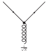
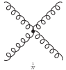
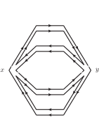
Quark and antiquark fields have color components, while gluon fields are matrix-valued fields with independent components111This approximation is justified because, as shown by ‘t Hooft[1], the traceless condition plays no role in the limit .. As a result, the gluon bubble diagram, Figure 1, brings a color factor since that is the number of possible intermediate gluon states. In contrast, a quark bubble diagram, Figure 1, brings a color factor being that the number of possible intermediate quarks. The interaction vertices and scale as – Figs. 1 and 1 – and the four-gluon vertex as – Figure 1. These factors appearing in the interaction vertices are a consequence of the rescaling of the coupling constant, , necessary to avoid further positive powers of in the perturbative expansion in the rescaled Yang-Mills coupling . For instance, the perturbative expansion in of the gluon propagator is at most of order although, at this order in , infinite diagrams with different orders in contribute.
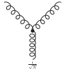
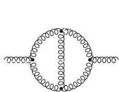
The simplest way to take properly into account all the combinatoric color factors is to introduce the ‘t Hooft double line representation[1]. As already observed, gluons are matrices, thus, as far as the color factors are concerned, they are indistinguishable from pairs when is large. For this reason one can substitute each gluon line with a couple of lines oriented in opposite directions. Examples of this representation are shown in Figs. 4, 4 and 4. The gluon self energy diagram in Figure 4 is of order : the factor is consequence of the two color loops and of the four interaction vertices.
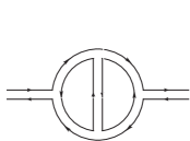
The diagram in Figure 4 is of order , arising from the vertices only. In fact, in the double line representation, this diagram has no closed fermion lines and hence no powers coming from loops. The comparison of this diagram with that in Figure 4 shows the difference between the weak-coupling and the Large- expansion: a sub-leading term in the former, Figure 4, is not so in the latter, Figure 4, and viceversa. Moreover, is a good expansion parameter regardless of the running of .
In Figure 4 it is shown an example of non-planar diagram. Non-planar means that it is impossible to draw it without line crossings. In this case the counting of color factors gives . Again, beside the vertices, the single factor of comes from the only fermionic closed line present in the diagram. It can be shown that this relative suppression of the non-planar diagrams compared to the planar ones is true in general. This is one of the most important simplifications induced by the Large- expansion.
The above discussion can be summarized in few important rules:
-
•
Planar diagrams with only gluon internal lines are all of the same order in the expansion.
-
•
Diagrams containing quark loops are subleading: the theory is quenched in the limit .
-
•
Non-planar diagrams are also subleading.
2.2 Weinberg’s observation
In his classic Erice lectures[3], Coleman justifies the non-existence of exotic mesons noticing that the application of local gauge-invariant quark quadri-linear operators to the vacuum state creates meson pairs and nothing else. The argument was as follows.
By Fierz rearrangement of fermion fields, any color-neutral operator formed from two quark and two antiquark fields
| (1) |
can be rewritten in the form
| (2) |
where are numerical coefficients and
| (3) |
is some generic color-neutral quark bilinear with spin-flavor structure determined by the matrix .
Let us look at the two-point correlation function of the operators, , and perform the fermonic Wick contractions first222This is always possible because the fermionic action is quadratic.. For simplicity, also suppose that the expectation value of single fermion bilinears vanishes, i.e. . The two-point function is a sum of terms that can be grouped in two different classes: double trace terms of the form
| (4a) | |||
| (4b) | |||
and single trace terms
| (5a) | |||
| (5b) | |||
where the flavor of the quark propagator is implied to simplify the notation. The subscripts and indicate a functional integration over the corresponding fields (gauge fields and fermions respectively). It is worth noticing that in the Large- limit the contribution in (4) has a perturbative expansion in of the form
| (6a) | |||
| (6b) | |||
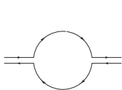
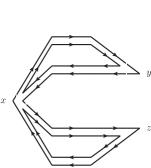
The first term of the right hand side in Eq. (6) is the product of two non-interacting meson bubbles (Figure 5, left panel) and is of order . The next-to-leading order term for this double trace contribution is the sum of planar diagrams like that in Figure 6

that are at most of order . For this reason we will refer to the leading contribution of this correlation function as “disconnected”, implying that there are no gluon lines connecting the two meson bubbles. The contribution in Eq. (5) is, instead, of order : in Figure 5, right panel, it is shown one of these possible single trace subleading terms (the shape of the diagram depends on the flavor structure of the quark bilinears). It is important to stress that the addition of any number of gluon lines internal to the fermion loops does not spoil the order of the diagram in the expansion because of the cancellation between the positive powers coming from the additional loops and the negative powers coming from the additional quark-gluon vertices. Therefore, as long as the expansion is considered, it will always be understood that any possible number of internal gluon lines, not changing the order of the expansion itself, will be included. Hence, since the leading order contribution to the single trace term in Eq. (5) is made of all the possible planar diagrams with internal gluon lines we will refer to it as the “connected” contribution. The complete two-point tetraquark correlation function can then be written as
| (7a) | ||||
| (7b) | ||||
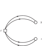
where the subscript “conn” stands for connected. The disconnected term contains only information about the propagation of two non-interacting mesons. This can be seen cutting in half the first diagram in Figure 5: assuming confinement, the only way to put on-shell the two bubbles is to form two non-interacting mesons. In contrast, there are different ways of cutting in half the second diagram of Figure 5 and it is possible to put on-shell simultaneously four quark propagators. For this reason, if a one-tetraquark pole exists, it contributes only to the connected term of the correlation function, which is of order , relatively vanishing if compared to the disconnected one, which is of order . Consequently, Coleman [3] concludes that such exotic mesons do not exist when .
However, Weinberg recently pointed out[4] that Coleman’s argument seems not to be conclusive. To make an analogy, consider the meson-meson scattering in the Large- limit. The scattering amplitude is dominated by the analogous of the disconnected term in Eq. (7), with the difference that all quark bilinears are now located in different points. Terms of interaction between meson bubbles are subleading in the expansion. This essentially means that, when , the mesons are non-interacting, but surely we do not infer that mesons do not scatter at all in the physical world, when . In other words, one should compute a scattering amplitude first and then take the Large- limit, otherwise the result would vanish right from the beginning, being the mesons non-interacting in this limit.
To better understand this point and what follows we will give some further details. Consider the scattering amplitude with , ingoing and , outgoing mesons:
| (8) |
where is the Fourier transform of the four-point correlation function
| (9) |
, are the two independent Mandelstam variables characterizing the scattering process. Moreover, can be expanded in the parameter , as the two-point function in Eq. (7). The renormalization constants bring a color factor of . This follows from the definition of in terms of the two-point function, , whose Fourier tansform reads:
| (10) |
where the dots stand for additional poles or cut contributions. Since the leading order contribution to is the bubble in Figure 1, with the insertion of any number of internal gluon lines not changing the -counting, it follows that
| (11) |
Therefore, the in Eq. (8) bring a factor of . As in Eq. (7), the leading disconnected contribution to is proportional to and hence it produces a term of order one in the amplitude. However, this term corresponds to a couple of freely-propagating mesons. For this reason, it doesn’t contribute to the cross section since it corresponds to the identity part of the -matrix, , that is subtracted in the LSZ formalism. The connected subleading term is, instead, of order and thus contributes as to the amplitude. This is the real leading term in the scattering matrix. On the other hand, if we had taken the limit first and applied the LSZ formalism after, we would have got because, as we mentioned, QCD in the Large- limit is a theory of non-interacting mesons and glueballs. In other words, taking beforehand kills all the contribution but the one describing the two mesons propagating without interacting.
In this spirit, Weinberg shows that, admitting the existence of a one-tetraquark pole in some connected correlation function of the kind mentioned above, the Large- expansion can actually be used to learn more about the phenomenology of tetraquark in the physical situation of finite . Consider the decay amplitude of a tetraquark into two ordinary mesons. As just observed, the quark bilinear entering in the LSZ formulation has to be normalized as . The same happens for tetraquark interpolating operators, where, for the connected term, holds
| (12) |
being the residue at the tetraquark pole. The properly normalized operator for the creations or annihilation of a tetraquark is , as for an ordinary meson.
The amplitude for the decay of a tetraquark is then proportional to a suitable Fourier transform, , of the three-point function
| (13) |
The disconnected term is leading and hence the decay width has a color factor proportional to . Therefore, it seems that tetraquarks would be very broad states, i.e. they would be unobservable in the Large- limit. However, when we amputate the tetraquark external leg,
| (14) |
this term vanishes: at leading order is just the convolution of two meson propagators, and thus contains meson poles only. Therefore the factor makes the amplitude vanish in the on-shell limit. On the other hand, if a tetraquark pole actually exists in the connected subleading term (the second term in (13)), it would have a decay rate proportional to and it would be stable in the Large- limit, just like an ordinary meson.
2.3 Flavor structure of narrow tetraquarks
In the previous section we showed that if a tetraquark exists, then it has a decay width proportional, at most, to . In this kind of analysis the flavor quantum numbers play a crucial role in predicting their decay widths.
Here we summarize some recent results about the classification of all possible flavor structures of tetraquarks[5]. In order to simplify the discussion, we define a quark bilinear with flavor quantum numbers and as
| (15) |
We will also assume that the flavor indices are different so that the vacuum expectation value identically vanishes. The tetraquark interpolating field will be denoted as
| (16) |
Since and , we have only three non-trivial possibilities for the flavor structure of the couple :
| (17) |
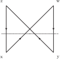
These three possibilities imply different quark contractions in the correlation functions involving tetraquark operators since contractions between different flavors are forbidden, and hence determine different Large- behaviors. The resulting predictions are summarized in Table 2.3 and can be derived looking at Figs. 9, 9 and 9. For a detailed derivation one should refer to the original work[5].
The remarkable aspect of this analysis is that a careful treatment of the flavor quantum numbers reveals the presence of even narrower tetraquarks than those decaying as . This happens in those situations in which the tetraquark is made out of quarks with all different flavors, for instance 333The notation is introduced to distinguish between a tetraquark written in the diquark-antidiquark basis – see Sec. 7 – against the notation – see Table 2.3.. Let us perform a detailed analysis for this case, the extension to the other flavor structures follows straightforwardly.
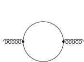
In order to determine the decay width of such a tetraquark it is sufficient to take only the leading connected contribution to the amplitude, in the sense specified in Sec. 2.2, with properly normalized operators. In this case, because (Figure 6) the color factor of is – also recall that the Large- order of must be evaluated from the two-point function as in Sec. 2.2. The color factor of the decay amplitude, Eq. (14), is:
| (18) |
where the color factor of is since the decay diagram of a tetraquark of this kind is analogous to Figure 9 – see again the original reference [5] for details. Finally, in this case a tetraquark-meson mixing is absent: cutting vertically the diagram in Figure 9 it is impossible to have a cut involving only two color lines, thus there is no meson intermediate state contribution. The decay width of this kind of tetraquarks goes as , being the decay amplitude of order , Eq. (18).
As a final note, we comment the Large- behavior of the diagram in Figure 9. At a first look, it seems a subleading non-planar contribution, since there are line crossings. However, the planarity is a topological property of the diagram, being its order associated to its Euler characteristic , as shown by t’Hooft[1, 3] , through the power law
| (19) |
where is the number of loops, the internal lines and the vertices of the diagrams. It hence follows that the one showed in Figure 9 is clearly a connected planar diagram (there are many examples of non-trivial planar diagrams, for instance in Maiani et al.[7]).
Flavor structure and associated decay width for tetraquarks as reported by Knecht and Peris [5]. The notation is used when the tetraquark is written in the meson-meson basis. Type Decay width Tetraquark-Meson mixing Example absent absent
2.4 Hypothetical non-perturbative contributions to tetraquark operators
In a recent paper by Lebed[8] a potential incongruence is found in considering the normalization of the tetraquark wave functions created by LSZ normalized operators.
The fact that is equivalent to the conclusion that LSZ reduction identifies the operator as the one creating or destroying properly normalized asymptotic states. This prefactor also produces correctly normalized meson states
| (20) |
Nevertheless, also – see Eq. (12), leading to a properly normalized tetraquark operator . However, its application to the vacuum creates states with norm squared
| (21) |
Lebed[8] pointed out that, in order to obtain the additional suppression needed for the correct normalization of the state in Eq. (21), the definition of the tetraquark operator as a local product of fermion bilinears must be revisited. We have already shown that, when the Large- limit is involved together with another different limit procedure, they must be treated carefully. In particular, in the LSZ formalism one has to take the infrared limit first, otherwise all the scattering amplitudes would identically vanish. In this spirit, one could ask if the Large- commutes with the definition of composite operators: an operation that involves a limit procedure. For example, in the scalar theory one may define the composite operator as
| (22) |
in order to obtain finite renormalized correlation functions with its insertions 444The operator product expansion is blind to contact terms of the form , for some power : an additional reason to define composite operators through a limit procedure..
Lebed[8] suggests that the non-commutativity of the limit and the local limit in the definition of the composite tetraquark operator is crucial in resolving the lack of the additional suppression factor in the tetraquark wave function in Eq. (21). Consider the product of operators
| (23) |
when 555We are ignoring the mixing with operators of dimension less than 6 because we are dealing with properly defined composite operators, Eq. (22). and allow the coefficients to have a contribution of the form
| (24) |
For any finite separation this contribution is vanishing when , in order to preserve the usual -counting for the correlation function of two mesons.
If one defines the tetraquark operator smearing the product over a small spatial region of size
| (25) |
the above mentioned four-point correlation function, in the limit , gets a contribution of for each spatial integral of the gaussian factor . If one obtains precisely the desired additional suppression in order to obtain properly normalized tetraquark wave functions.
We remark that the coefficients are non-perturbative in the -counting and cannot be inferred from perturbation theory. The mechanism proposed is only a possibility and there are no reasons to believe that it happens in this precise way. Nevertheless, it suggests that in order to allow the existence of one-tetraquark poles in the connected piece of the correlation functions considered so far, some non-perturbative mechanism in the expansion must occur.
2.5 Flavored tetraquarks in Corrigan-Ramond Large- limit
So far we discussed in detail the Large- physical behavior of meson and tetraquark states in the so-called ‘t Hooft limit[1]. Another well studied limit is that of Veneziano[9], with flavors, colors, provided that is fixed. In both these formulations, a simple definition of baryons does not exist, in contrast with what happens for mesons and tetraquarks. In fact, in generic gauge theories color-neutral states composed of only quarks – i.e. baryons – are made of quarks in a totally antisymmetric combination
| (26) |
As shown by Witten[2], they have very distinctive properties in the Large- limit. As already mentioned, their mass goes as , thus they disappear from the hadronic spectrum when .
As firstly proposed by Corrigan and Ramond[10], it could be important to have, for every value of , color-neutral bound states composed of only three quarks. A simple way to do it is to introduce new fermions, originally called “larks”[10], transforming as the (antisymmetric) representation of . This choice is motivated by the observation that, when , the dimension of this representation is and coincides with the conjugate representation
| (27) |
In this formulation, the baryons for Large- are constructed out of
| (28) |
color-neutral states, which look more like physical baryonic states. Moreover, just like quarks, larks only couple to gluons with a minimal coupling. The introduction of a lark sector in the Large- extrapolation of QCD, not only allows to define three-quark states, but also modifies the -counting. The reason is simple. If we introduce the ‘t Hooft double line representation[1] to understand the color flow of this theory, we notice immediately that lark lines split in two with arrows pointing in the same direction since both color indices in Eq. (27) belong to the same representation, in contrast with gluons, represented as two oriented lines pointing in opposite directions since their color indices always appear as a color-anticolor combination. Apart from the different orientation of the color flows, lark loops have a color factor like gluon loops. This implies that leading order planar diagrams contain any possible internal gluons as well as lark loop corrections to these gluon lines. In other words, we can also introduce an arbitrary number of lark “bubbles” in the middle of a gluon propagator. The reason is again simple: each insertion of a lark loop in a gluon line counts as but each lark-gluon vertex counts as and hence a lark loop in the middle of a gluon line does not change the -counting of the considered diagram – see Sec. 2.2. This is in contrast with quark loops, whose insertion inside a gluon propagator suppresses the order of the diagram in the expansion. For this reason we also see how including other antisymmetric tensors is dangerous for the expansion since they contribute in loops as , where is the number of antisymmetric color indices, thus spoiling the perturbative expansion of the correlators of the theory 666Larks can be considered as additional quark species: they couple to gluons with the same coupling constant of the quarks, but with the generators in the covariant derivative belonging to the antisymmetric representation. The same can be done for other species belonging to different representations of .. In fact, the fine cancellation between positive powers coming from loops and negative powers coming from couplings does not work for .
It was recently shown[11] that in the Corrigan-Ramond Large- formulation, i.e. the t’Hooft limit with quarks in the antisymmetric representation, (sometimes called QCD(AS)) it is possible to unambiguously define narrow tetraquark states. Consider a source operator of the form
| (29) |
where lowercase letters indicate color indices and are matrices in the Dirac and flavor space. Spin and flavor quantum numbers of the operator are fixed by a suitable choice of . This combination is gauge invariant, i.e. is a color singlet, if we notice that
| (30a) | ||||
| (30b) | ||||
under a generic gauge transformation . Moreover, lark color indices are saturated in such a way that the operator given by Eq. (29) can never be splitted into two independent color singlets for 777As already mentioned, the case is equivalent to the diquark-antidiquark formulation.. In other words, the two-point correlation function with sources as in Eq. (29) cannot be separated in disconnected pieces.
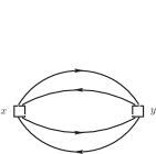
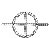
In Figure 10 we show the leading order contribution to the correlation function . Using the ‘t Hooft double line representation, Figure 10, we see that it is impossible to rearrange the colors in order to obtain two disconnected color singlet diagrams. This essentially means that operators like the one in Eq. (29) unambigously interpolate tetraquarks (or tetralarks in a generic ) states, without mixing with ordinary mesons.
Counting the lark loops we find that the color factor of this diagram is . As usual in the Large- expansion, the -counting does not change if we consider all the planar diagrams with the insertion of an arbitrary number of gluon internal lines. It is remarkable to notice again that this counting does not change even if we add any number of planar lark loops in the middle of these gluon lines for the reasons explained before.
At this point, we can easily show that an operator source like that in Eq. (29) can create out of the vacuum single tetralarks at leading order in the Large- expansion. We must be careful that, if the flavor of the sources allows lark-antilark annihilations, there are other diagrams besides that in Figure 10. In that case, however, it would not be possible to unambiguously disentangle the contribution of tetralark intermediate states from those of mesons. Imagine cutting vertically the diagram in Figure 10. Assuming confinement, the only way to form a gauge invariant combination of the lark lines involved in the cut is to group the four larks in a single hadron. This statement holds even if we insert an arbitrary number of gluon internal lines in the diagram in figure name 10. In that case the generic gauge-invariant contribution to the cut would have the form
| (31) |
with the gluon field. This is still a color-singlet combination with four larks. Since the two-point function brings a color factor (as shown by the power counting of Fig. 10) we also find that the LSZ properly normalized tetralark operators are . Since lark loops are not suppressed, there are also flavor-singlet contribution of states with an arbitrary number of lark-antilark couples. This means that the tetralark states found are not pure, but rather they are a superposition of infinite states, with arbitrary even number of larks, i.e. the analogous of “sea quarks” in the lark sector. However, they are unambiguously exotic states, since mesons made of larks cannot contribute to their two-point correlation function.
Finally, we show that tetralarks in the Corrigan-Ramond Large- limit are actually narrow states. To see this, consider the three point correlation function
| (32) |
where the operator interpolates a lark-antilark couple (we use the same notation of ordinary meson operators to stress the analogy among them). One of the leading order diagrams contributing to Eq. (32) is shown in Figure 11.
The counting of the color loops gives a factor , instead of obtained for the two-point correlation function of “tetralark” operators. Normalizing properly the amplitude, we obtain a total color factor , where we have used the result that is the LSZ normalized lark-antilark meson operator (we have not shown this, but it can be easily proven). The resulting decay width is then proportional to , showing that the in the limit Corrigan-Ramond tetralarks are narrow states.
2.6 Flavored tetraquarks in ‘t Hooft Large- limit
From a field theory point of view, it is a challenging task to identify operators interpolating only tetraquarks with flavor content . This is because such an operator would interpolate also mesonic states as having the same quantum numbers.
This is one of the major difficulties in treating these states using Lattice QCD, although some recent works on the subject has been presented [12, 13, 14, 15, 16]. Nevertheless, a class of operators that do not overlap with ordinary mesons and that unambiguously contain four valence quarks can be found[6].
It is the same class of operators already introduced in Corrigan-Ramond QCD(AS) formulation and considered in a recent work by Cohen and Lebed[17]. The authors show that the leading order connected diagrams contributing to the scattering amplitude of mesons with the appropriate exotic quantum numbers do not contain any tetraquark -channel cut. A careful and detailed analysis of the argument can be found in the original paper[17]. Here we will sketch the same argument referring to a specific case, in order to make the discussion more concrete.
Consider the following four-point correlation function – see Fig. 12 – that can be used, for instance, to compute the elastic scattering amplitude of mesons
| (33) |
with , , , appropriate Dirac matrices. We are looking for a possible -channel cut contributing to the four-point amplitude in which an on-shell tetraquark with flavor content propagates. We also notice that a -channel cut cannot reveal the presence of a tetraquark with these exotic flavor quantum numbers.
The current status of Large- tetraquarks. Coleman[3]/Witten[2] (1979) Tetraquarks do not exist, they are subleading in the large- QCD expansion. … … Weinberg[4] (2013) Even if subleading, tetraquarks can exist. In that case they are narrow as (like mesons). Knecht-Peris[5] Tetraquarks with 4 different flavors are as narrow as . Lebed[8] Non-perturbative effects in could affect tetraquark wave function. Cohen-Lebed 1[17] Tetraquarks naturally exist in Corrigan-Ramond limit (quarks in the antisymmetric representation). Cohen-Lebed 2[11] Production of tetraquarks in scattering amplitudes is only sub-subleading.
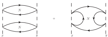
Imagine to cut the diagram in Figure 9 separating the incoming mesons in from the outgoing mesons in . The resulting cut is shown in Figure 12. Apparently, we are led to say that in the considered scattering amplitude there is a contribution from a tetraquark cut. However, drawing the diagram in a different, topologically equivalent, way (Figure 12), we see that the effect of the cut is to put on shell the corners of the diagram, thus separating all the meson sources from each other.
Recalling that the scattering amplitude is obtained, in momentum space, from Eq. (33) multiplying it for the inverse of the propagators of the mesons in the external legs, we have
| (34) |
with the Fourier transform of in Eq. (33). The factors cancel exactly the contribution of the sources to the -channel and the on-shell contributions come only from meson intermediate states.
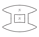
Drastically different is the situation for a tetraquark with flavor , as the recently discovered charged resonance . The resulting connected leading order diagram is similar to the diagram in Figure 9. In that case a cut in the -channel reveal either a meson or a tetraquark intermediate state.
To summarize, a pure tetraquark intermediate state, i.e. with flavor quantum numbers that can only be interpreted as exotic, cannot contribute to the leading order connected contribution to meson-meson elastic scattering amplitude. It is remarkable to notice that the experimental situation is drastically different. Until now, there is no evidence for such exotic resonances with all four different flavors and the considerations illustrated here are not applicable to the current experimental situation.
The key points of this section are schematically summarized in Table 2.6.
Sec. 3 Experimental overview
.
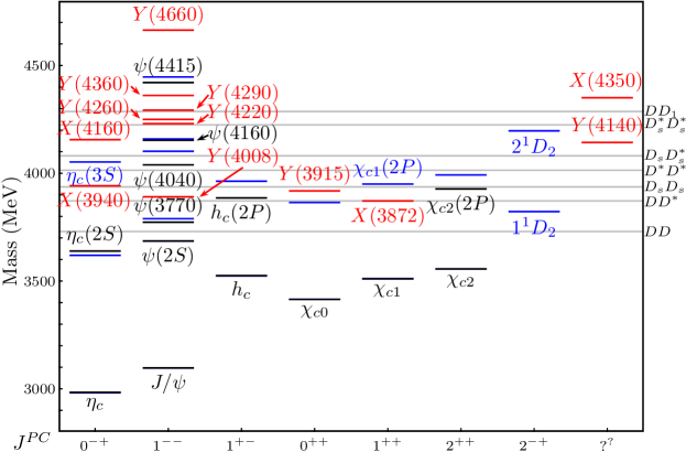
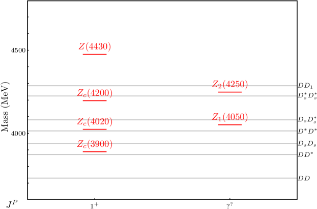
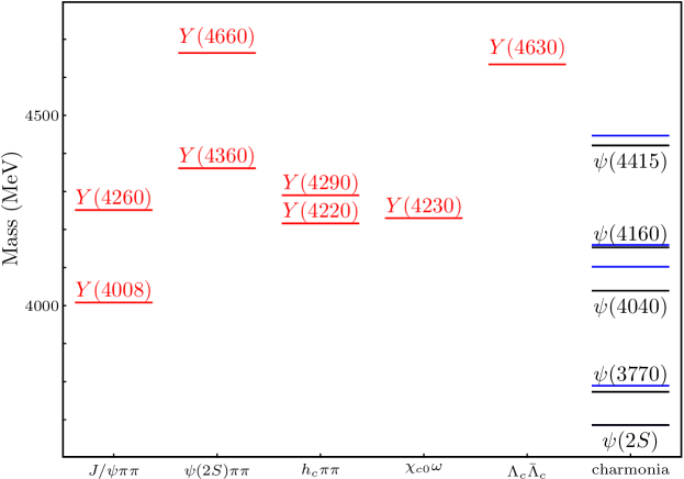
As shown in the previous section, recently a good deal of work has been done to understand the phenomenology of tetrquark states in Large- QCD. In particular, some doubts were raised about a possible broadness of these particles, that would make them experimentally undetectable. However, as we will show in the following sections, in the past eleven years many different experiments, both at lepton and hadron colliders, reported evidences for a large number of particles having properties which can hardly be embedded in the known charmonia frameworks. A pictorial representation of this is visible in Figure 13. In particular, the charged states reported in the second panel are manifestly exotic. Some states, like the or the , have more or less the correct mass and quantum numbers to be identified with (otherwise missing) ordinary charmonia; on the other hand, in the vector sector we have much more levels than expected. In any case, the decay pattern of these states is not compatible with charmonia predictions, and so it needs some exotic assignment.
Besides finding the states, the measurement of the quantum numbers is needed to establish their exotic nature. While prompt production at hadron colliders can produce particles with any quantum numbers, exclusive production modes, in particular at colliders, can constrain the assignment. For example, a generic state could be produced:
-
•
Directly with , if the center-of-mass energy coincides with the mass of the state (typically at - factories), or in association with Initial State Radiation (ISR) which lowers the center of mass energy, , typically at -factories. In the first case an invariant mass distribution can be studied by varying the energy of the beam, which does not allow to collect many data points with high statistics, while in the second the same distribution is studied as a function of the energy. In both cases, the quantum numbers must be the same as the photon, i.e. .
-
•
In the fusion of two quasi-real photons, , where and are scattered at a small angle and are not detected; the signal events have no tracks and neutral particles but the daughters of . If the photons are quasi-real, Landau-Yang theorem holds[19], and ; moreover is costrained.
-
•
In double charmonium production, for example , which constrains to have opposite to the one of the associated charmonium.
The production in decays allows to have any , albeit low values of the spin are preferred.
Hadron colliders, instead, produce charmonia states both directly and in decays, and the search is typically carried out inclusively.
A summary of the resonances we will talk about is reported in Table 3. We start our review from the charged ones, first the recently confirmed in Sec. 3.1, then we move to the charged states in the - region (Sec. 3.2) and the corresponding ones in the bottomonium sector (Sec. 3.3). The is extensively described in Sec. 3.4, as well as the vector states in Sec. 3.5. Finally, the other resonances around are described in Sec. 3.6, and the remaining ones in Sec. 3.7. Summary and future perspectives are in Sec. 3.8. Other information can be found in older reviews by Faccini et al.[20, 21]; a complete treatise about the physics of BABAR and Belle can be found in the recent review book[22].
Summary of quarkonium-like states. For charged states, the -parity is given for the neutral members of the corresponding isotriplets. State () () Process (mode) Experiment (#) Belle [23] (4.0) Belle [24, 25] (10), BABAR [26] (8.6) CDF [27, 28] (11.6), D0[29] (5.2) LHCb [30, 31] (np) Belle [32] (4.3), BABAR [33] (4.0) Belle [34] (5.5), BABAR [35] (3.5) LHCb [36] () BABAR [35] (3.6), Belle [34] (0.2) LHCb [36] (4.4) Belle [37] (6.4), BABAR [38] (4.9) BES III [39] (np) BES III [40] (8), Belle [41] (5.2) CLEO data[42] (5) BES III [43] (8.9) BES III [44] (10) Belle [45] (8), BABAR [46, 33] (19) Belle [47] (7.7), BABAR [48] (7.6) Belle [49] (5.3), BABAR [50] (5.8) Belle [51, 52] (6) Belle [53, 41] (7.4) Belle [54] (5.0), BABAR [55] (1.1) CDF [56, 57] (5.0), Belle [58] (1.9), LHCb [59] (1.4), CMS [60] (5) D [61] (3.1) Belle [52] (5.5) Belle [62] (7.2)
(Continued). State () () Process (mode) Experiment (#) BES III data[63, 64] (4.5) BES III [65] (9) Belle [54] (5.0), BABAR [55] (2.0) BABAR [66, 67] (8), CLEO[68, 69] (11) Belle [53, 41] (15), BES III [40] (np) BABAR [67] (np), Belle [41] (np) BES III [40] (8), Belle [41] (5.2) BES III [70] (5.3) BES III data[63, 64] (np) Belle [58] (3.2) Belle [71] (8), BABAR [72] (np) Belle [73, 74] (6.4), BABAR [75] (2.4) LHCb [76] (13.9) Belle [62] (4.0) Belle [77] (8.2) Belle [71] (5.8), BABAR [72] (5) Belle [78, 79] (10) Belle [78] (16) Belle [80] (8) Belle [78] (10) Belle [78] (16) Belle [80] (6.8)
3.1
In April 2014, LHCb confirmed the existence of a charged resonance in the channel[76]. 888Unless specified, the charged conjugated modes are understood. This announcement solved a controversy between Belle, which discovered[81] and confirmed[73, 74] the existence of this state, and BABAR, which did not observe any new structure and criticized some aspects of Belle’s analysis[75]. A state decaying into a charmonium and a charged light meson has undoubtly a four-quark content, being the production of a heavy quark pair from vacuum OZI suppressed. As we will discuss later, the very existence of such an exotic state far from usual open-charm thresholds is extremely interesting for phenomenological interpretations. We now briefly review the experimental history of this and other charged states.


The original Belle paper[81] studies the decays, and reports a peak in the invariant mass distribution, with and (Figure 14). This kind of analysis is particularly difficult, because the rich structure of resonances could reflect into the channel and create many fake peaks. However, Belle considered that the events with correspond to events with , i.e. an angular region where interfering partial waves cannot produce a single peak without creating other larger structures elsewhere. Belle named this state , and reported the product branching fractions
| (35) |
BABAR reviewed this analysis[75], by studying in detail the efficiency corrections and the shape of the background, relying for the latter on data as much as possible. Hints of a structure near appeared, even though not statistically significant, thus leading to a 95% C.L. upper limit on the production branching fraction
| (36) |

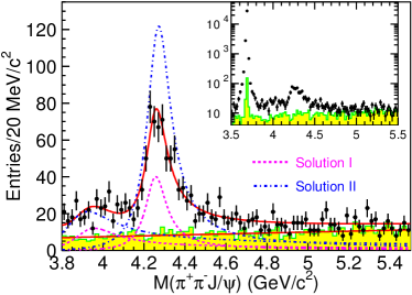
After that, Belle revised the analysis[73] studying in detail the 3-body Dalitz plot, and adding all known resonances, both with and without a coherent amplitude for the in the channel. Belle confirmed the presence of a peak with a statistical significance of . The Breit-Wigner parameter from the Dalitz analysis are and . A more recent 4D re-analysis by Belle [74] shows that the hypothesis is favored, modifying mass and width values to and (Figure 14). The production branching fraction is instead
| (37) |
LHCb confirmed this last result with a similar 4D analysis of the same decay channel. The is confirmed with a significance of at least, and the fitted mass and width are and . Also the signature is confirmed with high significance. The average à la PDG of Belle’s and LHCb’s mass and width are:
| (38) |
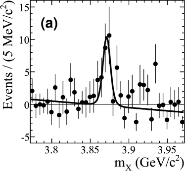
Since some theoretical papers[82] cast doubts on the resonant nature of the peak, in this analysis the complex value of the amplitude has been plotted as a function of (Figure 15). The behaviour is compatible with the Breit-Wigner prediction with the fitted values of mass and width. The same analysis also shows hints for a peak with quantum numbers likely , mass and width , ; however, since the Argand diagram is not conclusive about its resonant nature, LHCb has decided not to claim the discovery of another state.
Recently, Belle published a similar analysis of the decays[62]. Hints of a have been reported in invariant mass, with branching fraction
| (39) |
The fact that the is found in different decay channels gives solidity to its existence. In the same analysis, Belle claimed the discovery of a broad state with quantum numbers likely , mass and width , , with a significance of , possibly related to the LHCb hint. The reported branching fraction is
| (40) |
3.2 Charged states in the - region

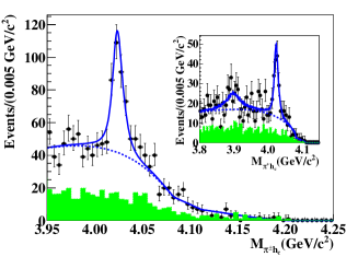
In March 2013, BES III [40] and Belle [41] claimed the discovery of a charged resonance in the channel at a mass of about , i.e. slightly above the threshold (Figure 16). BES III takes data at the pole, and analyzes the process ; Belle instead produces in addition with initial state radiation (ISR), and analyzes the process . The measured mass and width of the resonance are
| (41a) | ||||||
| (41b) | ||||||
and production branching fractions
| (42) |
This is the first time that a charged manifestly exotic state has been confirmed by two independent experiments, which has given some excitement to the charmonium community. The resonance was called . No measurement of quantum numbers has been performed, but is most likely if the decay is assumed to be in -wave. Soon after, an analysis of CLEO- data confirms[42] the presence of the charged in the decay and provides evidence for a neutral partner in the decay, with fitted parameters
| (43a) | ||||||
| (43b) | ||||||
A preliminary result by BES III confirm the existence of the neutral partner in [83]. A similar signal has been observed by BES III in , as a resonance in the invariant mass[39], with mass and width and (Figure 17). The signature is favored, and if this state is assumed to be the same as in the channel, we have
| (44) |
The resulting PDG averaged mass and width are[84]:
| (45) |
In the same period, BES III studied the process, and observed another charged resonance in the channel[44], at a mass slightly above the threshold, with quantum numbers likely . Soon after, BES III reported a similar peak in the reaction as a resonance in invariant mass[43]. This state is dubbed (Figure 18), and the measured masses and widths are:
| (46a) | ||||||
| (46b) | ||||||
| (46c) | ||||||
Moreover, BES III has recently reported some evidence for the neutral isospin partner , with and the width fixed to [85]. The is also searched[43] in the final state. A peak occurs at level, thus not statistically significant. A 90% C.L. upper bound on the production cross section is established:
| (47) | ||||
| to be compared with | ||||
| (48) | ||||
Similarly, no has been seen by BES III and Belle decaying into , as it is shown in Figure 16.
It is worth noticing that no has been seen by Belle in the channel[62], and the 90% C.L. upper bound on the branching fraction is:
| (49) |
Moreover, the COMPASS collaboration reported a search for , where the photon is obtained with scattering of positive muons at 160 and 200 on a target of LiD or NH3[86]. No signal is observed, and a 90% C.L. upper bound is put:
| (50) |
at .
In a Dalitz-plot analysis of decays, Belle could get an acceptable fit only by adding two resonances in the channel, which were named and [54]. The fitted masses and widths are
| (51a) | |||||||
| (51b) | |||||||
and reported the production branching fractions
| (52a) | ||||
| (52b) | ||||


The same decay was investigated by BABAR, which carefully studied the effects of interference between resonances in the system[55]. Considering interfering resonances in the channel only, BABAR obtained good fits to data without adding any resonance. Upper limits at 95% C.L. on the product branching fractions of and can be evaluated if incoherent resonant amplitudes for these two states are added to the fit:
| (53a) | ||||
| (53b) | ||||
Part of the discrepancy between the two experiments may be due to the fact that in the BABAR analysis the and terms are added incoherently and do not interfere with the amplitudes, while in the Belle analysis, significant constructive and destructive interference between the amplitudes and the resonances is more relevant (see the dips and peaks of the solid red curve in Figure19).
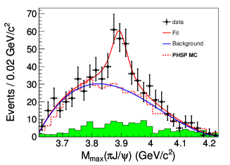
Finally, we report a peak in the invariant mass, in the full statistics analysis by Belle [87], with best fit parameters and .
3.3 Charged bottomonium states:

The and the could have their counterparts in the bottomonium sector. Belle reported the observation of anomalously high rates for the [88] and [89] transitions. The measured partial decay widths are about two orders of magnitude larger than typical widths for dipion transitions among the four lower states. Furthermore, the observation of final states with rates comparable to violates heavy-quark spin conservation. Belle searched for exotic resonant substructures in these decays[78]. In order to have a relatively background-free sample, the states are observed in their decay only, whereas the are reconstructed inclusively.
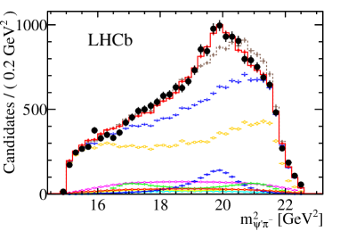
The Dalitz plots in the signal region (see for example Figure 20) is fitted with a sum of interfering resonances: the , the in channel, two new charged resonances in the channel, and a nonresonant background. The result of each fit is reported in Table 3.3; all the studied channels show the highly significant presence of both charged resonances, dubbed and , with compatible masses and widths. The one-dimensional invariant mass projections for events in each and signal region are shown in Figure 21. The average of all channels gives for a mass and width of , , and for a mass and width of , .
List of branching fractions for the and decays. From Belle [80]. Channel Fraction, %
The production rate is similar to that of the for each of the five decay channels. Their relative phase is consistent with zero for the final states with the and consistent with degrees for the final states with . Production of the ’s saturates the transitions and accounts for the high inclusive production rate reported by Belle [89]. Analyses of charged pion angular distributions[78, 90] favor the spin-parity assignment for both the states.


Comparison of results on and parameters obtained from and analyses[78]. Final state , , , , Rel. normalization Rel. phase, degrees
Belle searched these states also in pairs of open bottom mesons[80]. The Dalitz plots of and report a signal of and a signal of , respectively, whereas is compatible with zero999 is phase-space forbidden.. The best estimate for the branching ratios are reported in Table 3.3.
Recently, Belle has been able to find the neutral isospin partner [79] in decays, at a significance of if mass and width are fixed to the averaged values of the . If the mass is let free, the fitted value is , consistent with the charged partner mass. On the other hand, no significant signal of is seen.
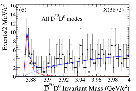
3.4 The saga
The queen of exotic states is the . It was discovered by Belle while studying the decays[24], as an unexpected resonance in the invariant mass distribution (see Figure 23, left panel). It was then confirmed both in decays[91] and in inclusive prompt [92, 29] and production[30, 93] – see Sec. 6 for a long-standing controversy about the theoretical interpretation of that. First of all, an exotic nature was suggested by its narrow width, at 90% C.L.[24], despite being above threshold for the decay into a charmed meson pair. Furthermore, both invariant mass distribution[24, 94] and angular analyses[27] show that the amplitude is dominated by the meson, i.e. a resonance. If the were an ordinary charmonium with , such a decay would badly violate isospin symmetry. The size of isospin breaking was quantified by the measurement of the branching fraction by Belle [32] and BABAR [33]:
| (54) |
The assignment was confirmed by the observation of the decay[32, 95], and by the non-observation of [24]. As for the spin, a preliminary angular analysis of the by Belle [96] favored assignment. Soon after, a more detailed analysis by CDF [27] was able to rule out all but the and assignments. The latter could not be excluded because of the additional complex parameter given by the ratio between the two independent amplitudes for , which could not be constrained in inclusive production; on the other hand, the former was preferred by theoretical models. Instead, the analysis of the invariant mass distribution by BABAR [33] favored the hypothesis, and stimulated a discussion on its theoretical feasibility[97, 98, 99, 21, 100]. However, a assignment would allow to be produced in fusion, but CLEO has found no significant signal in [101]. A statistically improved analysis of angular distributions in has been made by Belle [25], again favoring . The limited statistics forced Belle to consider three different one-dimensional projections of the full angular distribution, which were not able to rule out .
Finally, LHCb has recently published an analysis of a large sample[31]. This study is based on an event-by-event likelihood ratio test of and hypotheses on the full 5D angular distribution, and favors the over at level. The additional complex parameter in the distributions is treated as a nuisance parameter; its best value extracted from the fit is found to be consistent with the value obtained if the events are MC generated with a assumption; this is consistent with the Belle’s result too[25]. It is worth noticing that the only analysis which favored the assignment was the BABAR analysis and an independent analysis of the same channel by other experiments would be very interesting.

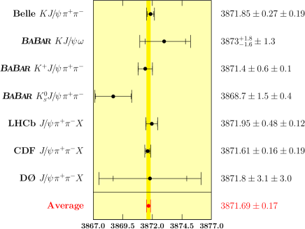
In Figure 22 we report a list of the most recent mass measurements. The current world average, considering only decays into final states including the , is [84]. The most precise measurements are those of CDF [28], Belle [25], the new measurement from LHCb [30], and BABAR [26], all in the channel ; the hadronic machines measure inclusive production in , while the -factories measurements are dominated by .
Belle observed the decay in the final state at the higher mass [102]. This was confirmed by BABAR [38] (see Figure 23, right panel) and again by Belle [37], leading to an average mass of . As this is significantly larger than the value observed in the discovery mode , there has been some discussion about the possibility that and are distinct particles. However, some papers[103, 104, 105] argued that, since the will in general be off-shell, a detailed study of the and lineshapes is needed to distinguish between a below- and above-threshold (see Sec. 5.1.1). Moreover, in order to improve the resolution, the experimental analyses constrain the mass, and this yields to a reconstructed mass which is above threshold by construction. Because of these biases, this channel has been dropped from mass averages in PDG[84].
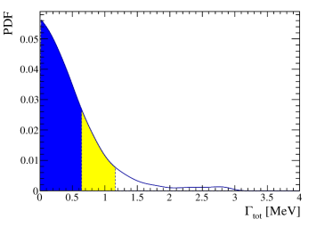
As far as the width is concerned, the was known to be narrow since the very first analysis, with a limit at 90% C.L.[24]. The best current upper limit for the width is given by Belle [25], which finds at 90% C.L. based on a 3D fit to , , and , which allows the limit to be constrained below the experimental resolution on invariant mass: the distributions in and provide constraints on the area of the peak, which make the peak height sensitive to the natural width.
In addition to and final states, the has been sought in many other different channels, which we list in Table 3.4.
We just discuss the case of , which is of interest for theoretical interpretations. BABAR [35] and LHCb [36] find a signal with a relative branching fraction of:
| (55a) | ||||
| (55b) | ||||
| (55c) | ||||
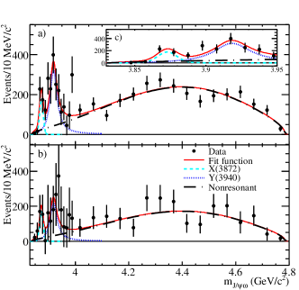
In particular, for the decay , Belle [34] sees no significant signal and puts a 90% C.L. upper limit (see Figure 24).


Other production mechanisms like have also been studied. Such decays are seen, but with a smooth distribution in invariant mass; an upper limit is set on [106]. This is in contrast to ordinary charmonium states, where and branching fractions are comparable, and dominates over nonresonant . We also mention the decay seen by BES III [70], with a production cross section of .
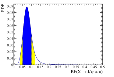
In Table 3.4 we update the results of Drenska et al.[20] on the absolute branching fractions of the . These can be obtained from measured product branching fractions of by exploiting the upper limit on measured by BABAR from the spectrum of the kaons recoiling against fully reconstructed mesons[107], at 90% C.L.. Combining the likelihood from the measurements of the product branching fractions in the observed channels, the upper limit and the width distribution[41], with a bayesian procedure we extracted the likelihood for the absolute branching fractions and the widths in each of the decay modes. Then, we used the probability distributions obtained with this procedure to set limits on the not observed channels. The full shape of the experimental likelihoods was used whenever available, while gaussian errors and poissonian counting distributions have been assumed elsewhere. The 68% confidence intervals (defined in such a way that the absolute value of the PDF is the same at the upper and lower bound, unless one of them is at the boundary of the physical range) are summarized in Table 3.4 for each of the decay modes. Some of the likelihoods are shown in Figure 25.


The searches for partner states of the have been motivated by the predictions of the tetraquark model (see Sec. 7). For example, it has been hypothesized that the state produced in decays was different from the state produced in decays. If so, the two should have different masses. Both BABAR [108, 26] and Belle [106, 25] have performed analyses distinguishing the two samples. The most recent results set the mass difference of the two at
| (56a) | ||||
| (56b) | ||||
| (56c) | ||||
Moreover, an inclusive analysis by CDF [28], of the spectrum, gives no evidence for any other neutral state, setting an upper limit on the mass difference of at the 95% C.L..
The same analyses provide measurements of the ratio of product branching fractions
| (57a) | ||||
| (57b) | ||||
Searches for charged partners have also been performed by both BABAR [109] and Belle [25]. No evidence for such a state is seen, with limits on the product branching fractions of
| (58a) | ||||
| (58b) | ||||
| (58c) | ||||
| (58d) | ||||
to be compared with
| (59a) | ||||
| (59b) | ||||
for the discovery mode, measured by BABAR [26] and Belle [25].
Measured product branching fractions, separated by production and decay channel. Our averages are in boldface. The last two columns report the results in terms of absolute branching fraction () and in terms of the branching fraction normalized to () as obtained from the global likelihood fit described in the text. For non-zero measurements we report the mean value, and the 68% C.L. range in form of asymmetric errors. The limits are provided at 90% C.L. The is dominated by , but no limits on the non-resonant component have been set. The ratio given by LHCb [110] is the ratio . decay mode decay mode product branching fraction () (BABAR [26], Belle [25]) 1 BABAR [26] Belle [25] (BABAR [26]; Belle [25]) BABAR [26] Belle [25] Belle [106] , 90% C.L. Belle [106] BABAR [33] BABAR [33] BABAR [33] Belle [32] (BABAR [38]; Belle [37]) BABAR [38] Belle [37] (BABAR [38]; Belle [37]) BABAR [38] Belle [37]
We conclude this section on the with the inclusive production at hadron colliders: the prompt production has been studied at CDF [113] and CMS [93], giving
| (60a) | ||||
| (60b) | ||||
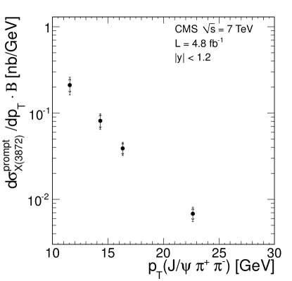
CMS published also the value for the prompt production cross section, at (see Figure 26).
The same measurement is not present in the CDF note, but it has been estimated by Bignamini et al.[114]: at .
3.5 Vector resonances
Many states with unambiguous have been discovered via direct production in collisions. The -factories can investigate a large mass range, by searching events with an additional energetic photon emitted by the initial state, which lowers the center-of-mass energy down to the mass of the particle. The factories can instead scan the mass range by varying their center-of-mass energy. A graphic summary of all this states is in Figure 27.
In 2005 BABAR observed an unexpected vector charmonium state decaying into named [66], with a mass of and a width of . Soon after it was confirmed by CLEO [69, 68], which reported evidence also for . BABAR performed a similar analysis in the channel[115], finding no evidence of ; instead, a heavier state was observed at a mass and a width , dubbed . The absence of is significant: at the 90% C.L.[116], and is hard to understand in an ordinary charmonium framework. This pattern has been confirmed in an update of BABAR’s analysis[72].
Belle confirmed both these vector states[53, 71], and observed another resonance, called , in the channel, which BABAR was not able to see because of limited statistics, with mass and width . It also found a broad structure in named , at mass and width . This last state has not been seen by BABAR [67], but it has been confirmed in the full statistics analysis by Belle [41], with and . The PDG[84] averaged mass and width for the are based on the most recent analyses by Belle [41], BABAR [67] and CLEO [69] and are and . The full statistics analysis in by Belle [87] gives for the a mass and width of and , and for the a mass and width of and . In Figure 28 we report some distributions of and by Belle.

Motivated by the tetraquark predictions, Belle searched for vector resonances decaying into [77]. A structure (the ) has actually been found near the baryon threshold, with Breit-Wigner parameters and . A combined fit of the and spectra concluded that the two structures and can be the same state, with a strong preference for the baryonic decay mode: [116].
The vector states mentioned before are considered to be exotic. In fact, there are no unassigned charmonia below , and the branching ratios into open charm mesons are too small for above-threshold charmonia: BABAR sees no evidence for a signal[117, 118], and set 90% C.L. upper limits:
| (61a) | ||||
| (61b) | ||||
| (61c) | ||||
| (61d) | ||||
| (61e) | ||||
| (61f) | ||||
whereas the limits set by Belle [119] are:
| (62a) | ||||
| (62b) | ||||
| (62c) | ||||
to be compared with for an ordinary above-threshold vector charmonium. As for radiative decays, has been observed by BES III. Some clean events of have been measured. Moreover, the production cross section scales as a function of the center-of-mass energy consistently with a Breit-Wigner with mass and width as parameters, consequently the observed events come from the intermediate resonant state and not from the continuum. The has been searched without success in many other final states, which we report in Table 3.5.
Another important question to understand the nature of these vector states is whether or not the pion pair comes from any resonance. The updated BABAR analysis in [67] finds some evidence of a component. Since the decay is phase-space forbidden, this could partially explain why the does not decay into (although the relevant non-resonant component could allow this decay). Some indications of an component in the appear in Belle’s analysis[71], while no definite structure is recognizable for the other resonances.

BES III also measured the cross sections at center-of-mass energies varying from to [43] (see Figure 29). The values of the cross sections are similar to the , but the line shape is completely different and does not show any signal for the . The has been fitted by Yuan[63, 64], which found a significant signal for a new state. The fit improves if a second resonance is added, however the lack of experimental data above makes hard to distinguish this second peak from a non-resonant background. The values of the mass and width according to the one peak hypothesis are and . If there are two peaks, the best fitted values are , and , .
A somewhat similar signal has been seen by BES III in [65] at a mass of and a width of , again not compatible with parameters.
3.6 The family
Some resonances with have been observed around . Even if they could be likely interpred as ordinary charmonium states, some peculiarities in their decay patterns favor a more exotic assignment.
The was observed by Belle in double-charmonium production events as a peak in the recoiling mass[51, 52], with and . A partial reconstruction technique in this production channel showed that is a prominent decay mode (see Figure 30, right panel), whereas show no signal. The production mechanism costrains the state to have . All known states observed via this production mechanism have , so a tentative assignment for this state is , where the parity is suggested by the absence of decays.
Belle observed another state at a similar mass in decays as a resonance in the invariant mass, with and [45]. The fact that such a state is not seen in strongly suggests that it is not the , whence it was dubbed . The decay into two vectors costrains a assignment, whereas and are equally allowed. BABAR confirmed the state in [46, 33], even if at a lower mass and with narrower width, and , compatible at level with Belle measurement (see Figure 30, left panel). This discrepancy could be due to different assumptions about the shape of the background. Another state called was observed in fusion by both Belle [47] and BABAR [48], with mass and width compatible with the BABAR result. The PDG, which assumes the resonances seen in fusion and in decays to be the same state (called ), gives an averaged mass and width of and [84]. The study of angular correlations by BABAR favors a assignment[48], which would make this state a candidate for . However, the is expected to have , i.e. wider than the total width measured of the . Even if no upper bound on has been reported, no signs of a signal for such a decay appear in the measured invariant mass distributions for decays published by BABAR [38] and Belle [126]. Moreover, if the (see below) is identified as the state, the hyperfine splitting would be only with respect to the splitting. This is much smaller than the similar ratio in the bottomonium system (), and than the potential model predictions[127] (). These facts challenge the ordinary charmonium interpretation[128, 129].
Another state, at the time called , was seen by Belle in [49], and confirmed by BABAR [50], at an averaged mass and width of and . The angular analysis by BABAR favors a assignment. This state is compatible with the assignment.

3.7 Other states
The analysis by Belle of double charmonium events which discovered the observed also a state called in the invariant mass[52] (see Figure 30, right panel). The fitted mass and width are and . The production mechanism costrins and favors , thus making this state a good candidate for a a state.
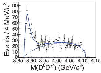
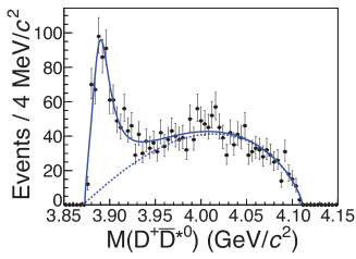
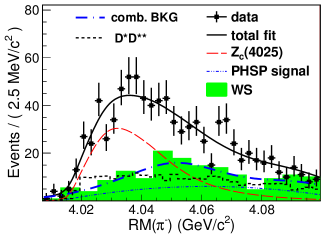
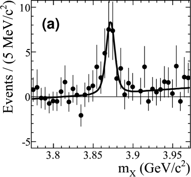
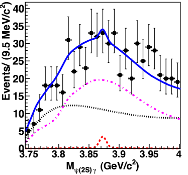
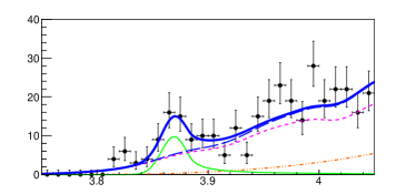
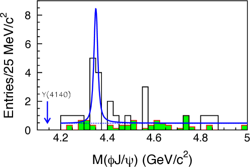
The CDF experiment announced a resonance close to threshold in invariant mass, in the channel [56, 57]. Since the creation of a pair is OZI suppressed, the very existence of such states likely requires exotic interpretations. This state is called , and has mass and width and . The natural quantum number would be , but the exotic assignment is not excluded. Belle searched this state in fusion, driven by a molcular prediction[130], but found no signal and put a 90% C.L. upper bound for for [58]. Instead, a peak with a significance was seen at and (see Figure 31), and dubbed .
Several experiments have searched for the : D [61] and CMS [60] have recently confirmed the observation, and reported mass and width , and , with significances of and , respectively. On the other hand, neither LHCb [59] nor BABAR [131] are able to see any significant signal, and put 90% C.L. upper limits on the relative branching fractions of
| (63a) | ||||
| (63b) | ||||
to be compared with a measured by CMS. We mention also a preliminary null result of BES III in the invariant mass in process[132].
The averaged values of mass and width à la PDG[84] from the experiments that have claimed the observation are and .
Last state we review is the seen by Belle in radiative decays, with mass and width of and at 90% C.L., with a significance of [23]. Nothing prevents the identification of this state as the ordinary charmonium.
3.8 Summary
We show in tabular form the state-of-the-art of experimental searches of exotic states, organized by production mechanism: decay (Table 3.8), direct production (with or without ISR, Table 3.8), double charmonium production (Table 3.8), and two-photon production (Table 3.8); studies of charged states are summarized in Table 3.8. It appears that our knowledge is quite fragmentary: all exotic resonances but the and the have been observed in one production mechanism only, and many in one final state only. Analyses of particular combinations of production mechanism and final state are missing, or not performed in the relevant range of invariant mass, or there is no fit to the data to test for the presence of already discovered exotic states. To conclude, a systematic study of the exotic spectrum is needed to form a definite experimental picture of these states and their structure. New results from the LHC and from high-luminosity - and - factories will be important to settle our understanding of this sector.
Status of searches for the new charged states, for several final states , updated with respect to Drenska et al.[20]. The meaning of the symbols is explained in the caption of Table 3.8. For these states we expect parity to be conserved in the decay. Charged states State — NS — — MF — NP MF — S — MF — — NS NP S — MF NP MF NP MF MF NP NP — NS NP MF — — S NP NP S MF NP MF NP S MF NP NP MF MF NP MF NP MF NP NP NP MF S — MF — — NP NP S — MF NP MF NP S NP NP NP MF MF NP MF NP MF — NP NP MF S — S — — NP NP NP MF
Status of searches for the new states in decays, for several final states , updated with respect to Drenska et al.[20]. Final states where each exotic state was observed (S: “seen”) or excluded (NS: “not seen”) are indicated; F is reserved to final states which have been searched and not seen, but are forbidden by quantum numbers not known at the time of the analysis. A final state is marked as NP (“not performed”) if the analysis has not been performed in a given mass range and with MF (“missing fit”) if the spectra are published but a fit to a given state has not been performed. Finally “—” indicates that the known quantum numbers or available energy forbid the decay; and “hard” that an analysis is experimentally too challenging. As explained in Sec. 3.6, we consider a state decaying into , seen both in decays and in fusion, and a state seen in double charmonium production and decaying into . “Vectors” indicates the states discovered via ISR not explicitly mentioned in the table.
| State | |||||||||||||||||
|---|---|---|---|---|---|---|---|---|---|---|---|---|---|---|---|---|---|
| S | S | S | — | F | — | — | S | F | NS | — | — | S | — | — | F | ||
| MF | S | NS | — | — | — | — | MF | — | MF | — | MF | NS | — | NP | NP | ||
| MF | MF | NS | — | — | — | — | MF | — | MF | — | MF | MF | — | NP | NP | ||
| MF | MF | NP | S | — | NP | — | NP | — | MF | — | MF | NP | NP | NP | NP | ||
| MF | MF | NP | MF | — | NP | — | NP | — | MF | — | MF | NP | NP | NP | NP | ||
| MF | MF | NP | MF | — | NP | NP | NP | — | MF | — | NP | NP | NP | NP | NP | ||
| NS | — | — | — | MF | NP | — | — | NP | MF | — | NP | NP | NP | NP | — | ||
| vectors | MF | — | — | — | MF | NP | — | — | NP | MF | — | NP | NP | NP | NP | — | |
| NP | — | — | — | MF | NP | — | — | NP | MF | MF | NP | NP | NP | NP | — | ||
Status of searches for the new states in ISR produtcion for several final states , updated with respect to Drenska et al.[20]. In this table we consider the decaying into and the decaying into to be the same state. The meaning of the symbols is explained in the caption of Table 3.8. , State S MF MF MF MF — MF MF — MF MF MF MF MF MF S MF MF S MF MF — MF MF MF MF S NS NS NS NS NS NS MF — NS NS NS NS MF NS S NS NS NS MF MF — MF MF MF MF NS S MF MF MF MF MF MF — MF MF MF MF NS S NP MF MF MF MF MF S MF MF MF MF
Status of searches for the new states in double charmonium production events, for several final states , updated with respect to Drenska et al.[20]. We tentatively assign to because of the lack of decay mode. The meaning of the symbols is explained in the caption of Table 3.8. , State hard NP hard — hard — hard hard hard hard — MF MF — hard NP hard — hard — hard hard hard hard — F S — hard NP hard — hard — hard hard hard hard — MF MF — hard NP hard NP hard — hard hard hard hard — MF MF MF hard NP hard NP hard — hard hard hard hard — MF S MF hard NP hard NP hard NP hard hard hard hard hard MF MF MF \tblStatus of searches for the new states in fusion, for several final states , updated with respect to Drenska et al.[20]. The meaning of the symbols is explained in the caption of Table 3.8. , , State F — — — — — — — — — — — — — NP S hard — — — hard MF MF — MF NP — NP NP MF hard — — — hard MF MF — S NP — NP NP MF hard NS NP — hard NP NP — MF NP NP NP NP MF hard NS NP — hard NP NP — MF NP NP NP NP NP hard S NP NP hard NP NP NP NP NP NP NP
Sec. 4 Lattice QCD status of exotics
Lattice QCD has recently reached some preliminary results about exotics, albeit the non-trivial numerical and theoretical difficulties. In fact, from a field theoretical point of view, there is no way to distinguish between a meson and a tetraquark with the same quantum numbers, as we discussed for Large- QCD (see Sec. 2). For instance, the charged resonance , with quark content , has the same quantum numbers as the (the lightest axial vector), so that any operator able to resolve the interpolates also the excitations of . In principle, the existence of the can be revealed by extracting all the excited levels up to the mass of the , but this is not numerically feasible. A numerically reliable approximation, widely used in heavy quarkonium spectroscopy, is to neglect charm annihilation diagrams[133], which are expected to be small because of OZI suppression. Under this approximation, it is possible to deal with these states using a field theory approach. In current lattice simulations one considers the vacuum expectation value of two-point functions for a set of interpolating operators with given quantum numbers. For each of them, the spectral representation gives
| (64) |
From a single correlation function it is possible to extract only the lowest lying state using the effective mass method: when the time is large, the function
| (65) |
has a plateau at the energy of the ground state. The excited energy levels are extracted using the generalized eigenvalue problem[134]. If we have different operators with the same quantum numbers, we can compute the correlation function matrix , (). The solution of the eigenvalue problem
| (66) |
gives levels of the energy spectrum: in fact, the resulting eigenvalues decay exponentially with the energy level, up to exponentially suppressed deviations:
| (67) |
The larger is the basis of operators, the larger is the number of computable excited levels. For numerical reasons, the operators have to be also as different as possible. If we were interested in below-threshold states, this is enough. If we instead are interested in above-threshold resonances, we have to look at all 2-particle levels with the same quantum numbers as the resonance. While at infinite volume these levels form a continuum101010In fact, no information about resonances can be deduced from Euclidean correlators in the thermodynamic limit[136]., on the lattice these levels have a rather peculiar behavior as a function of the size of the volume. In particular, their energy is related to the infinite volume scattering phase[137, 138]. Roughly speaking in fact, by varying the size of the lattice, we vary the relative momentum of the 2-particle states (), hence we simulate a “scattering” experiment at different momenta.
Currently, the only positive result in charmonium lattice spectroscopy is the confirmation of an energy level compatible with the in the channel with isospin [13] – see Figure 32. It is argued that the energy level found on the lattice is a real shallow bound state because of the large positive shift in energy of the state [139]. The signal of a level below the threshold seems to indicate the presence of the in QCD spectrum. It is worth noticing that this result is very sensitive to lattice artifacts, in particular the charm mass (and consequently the threshold) is affected by large discretization effects: for example this level could go away from threshold when approaching the physical point. Moreever, there is no way to distinguish such state from the ordinary : even if the level were confirmed, Lattice QCD cannot say whether it has the exotic features of the .

For the sector with the situation is still unclear: the analysis of the energy levels does not reveal any additional state, expected in presence of a resonance[135, 140] (Figure 33). However, this level could be obscured by the presence of many different two-particle mesonic channels.
Furthermore, the above-mentioned approximation of neglecting charm annihilation contributions, unavoidable in practice, could make tetraquark states hard to be found. This statement is motivated by a Large- analysis. Consider the 2-point correlation function . The leading and subleading contributions to this correlation function are shown in Figure 34. In Sec. 2.6, we showed that both the disconnected and the crossed diagrams (first and third in Figure 34) receive contributions from two meson states only. However, a tetraquark pole could appear in (subleading) diagrams which present any quark annihilations (second in Figure 34). Such kind of diagrams are neglected in simulations (it is not numerically feasible to take into account charm annihilation), whereas in the channel the light quarks are able to annihilate. This suggests that the possible tetraquark pole could be out of reach of current simulations.
Sec. 5 Phenomenology
5.1 Molecule
Soon after the first observation of the in 2003, its closeness to the threshold suggested to many authors that it might be the very first example of a loosely bound meson molecule. The possible existence of such states has been proposed many years ago by Tornqvist[141, 142] looking for hypotetical , , , etc. bound states. It has been argued that the one-pion-exchange potential is likely to bind some states composed of ground state mesons, the idea being driven by the analogy with the time-honored case of deuterium where one knows that this potential is the dominant one. The same idea can also be extended to the heavy sector[143, 144, 145, 146]. In particular, it has been found[145] that one-pion-exchange alone is strong enough to form at least deuteron-like and states with binding energy of abount MeV. Composites made of and and bound by pion exchange alone – i.e. neglecting the contribution from other kinds of potential – are expected near threshold, while molecular states composed of light mesons would require a stronger additional short range attraction and hence are likely not to be formed if only pions are taken into account.
Using an effective Lagrangian for pions one can find the following potentials in momemtum space for the interaction between pseudo-scalar () and vector () mesons[145]:
| (68a) | ||||
| (68b) | ||||
where MeV is the pion decay constant and is some axial effective strong coupling. are the spin-1 matrices, are the Pauli isospin matrices and is the polarization vector for the vector meson. It should be stressed that the potential is forbidden by parity conservation. It is worth noticing that, in coordinate space, the potential is singular, and needs an ultraviolet cutoff . The existence of loosely bound molecules can crucially depend on the choice of the cutoff[141, 147, 148].
In Table 5.1 we report the expected bound states according to this one-pion-exchange framework[149]. As one can see the would perfectly fit into this picture. This motivated a great ammount of work done on the topic. In the following sections we will present some phenomenological models and their consequences, assuming these exotic states to be mesonic molecules.
Bound states expected by the one-pion-exchange model[149]. The masses are predicted to be near threshold for the case of mesons and about 50 below threshold in the case of mesons. All states have isospin . Bound state Mass [MeV] Bound state Mass [MeV]
A somehow complementary approach was established by Barnes and Swanson[150, 151]: meson-meson interactions can be obtained as the sum of effective potentials between the constituent quarks of the mesons. The hamiltonian is given by
| (69a) | ||||
| (69b) | ||||
where is the one-gluon exchange potential at Born level, is the (non-perturbative) linear potential which takes into account confinement, and parametrizes the hyperfine splitting of the charmonium levels. Even if constituent quark models are commonly used in quarkonium physics, it is unclear whether they can describe strong interactions on the scale of loosely bound molecules (); it is more likely that quark can interact with each other on the typical scale of strong interactions, i.e. , but if so, the distinction between hadronic molecules and tetraquarks would become just a matter of language, the only difference between the two being the way in which color is saturated. It is worth noticing that this interaction is not strong enough to bind the , and a contribution from one-pion-exchange has to be added[152].
Finally, in the heavy sector one can use heavy quark spin symmetry to obtain predictions for molecular spectrum and decay patterns, regardless of the details of the binding potential [153, 154, 155].
5.1.1 Low-energy universality and line shapes of the
As we mentioned before different potential models predict the presence of bound molecular states. Among these possible molecules the , interpreted as an -wave state, would have a whole set of striking features due to the closeness to its constituents threshold. Its binding energy (simply given by the difference between its measured mass and the mass of its constituents) would be[156] MeV. The natural energy scale for a pionic interaction is given by MeV and hence is much larger than .
Bound states with such a feature share some common properties – the so-called low-energy universality111111 It should be mentioned that low-energy universality has been exploited for the first time by Voloshin[157] to compute the momentum distribution for the and decays. – coming from non-relativistic Quantum Mechanics and, in particular, many of their characteristic can be described via a single parameter: the scattering length, . When the scattering length gets bigger and bigger (or analogously when the binding energy, , gets smaller and smaller) we have that
| (70) |
For the case of the we have MeV and this leads to an unusually large scattering length, fm fm, the last one being the typical range of the interaction between the two mesons121212 It has been shown[158] that the scattering lenght obtained with this formalism can hardly be reconciled with the one obtained by the experimental data on the width, which appears to be smaller by (at least) a factor of .. Such a striking feature necessarily requires some kind of fine tuning. Moreover, the wave function for the constituents assumes the universal form
| (71) |
Note that this also implies that a loosely bound molecule is an extremely extended object, having a typical radius .
It has been pointed out[159] that the most generic quantum mechanical state for the can be written as
| (72a) | ||||
| (72b) | ||||
where is the wave function of the mesons in momentum space and are other possible states (discrete or continuous) having the same quantum numbers , e.g. or . The constants are the probabilities for a certain configuration. Using an effective field theory approach, it can be shown[159] that such suppression factors go as , where is the energy gap between the state and the threshold.
Two mechanisms to explain the large scattering length of the has been proposed[159]:
-
1.
If all the other states have an energy gap then, for a fairly large , and , i.e. the would be purely a molecule. In this case the fine tuning necessary to explain the value of would be something related to the interaction between the two components only, e.g. the depth or the width of the potential or the mass of the mesons. In particular, one can consider as a tuning parameter since it influences both the one-pion potential and the mass of the two mesons.
-
2.
If one of the states has mass very close to the threshold, the factor would compensate the suppression due to the scattering length and lead to an almost equal mixture of this state and of the molecule, . This mechanism is the analogous of the well-known Feshbach resonances which are used in atomic physics to control the scattering length[160]. It has been hypotesized that this state might be the (still undiscovered) charmonium . However, potential models predict the mass of this particle to be MeV above the threshold and hence we would need a fortuitous shift of this by at least MeV, in order to achieve .
Since the second mechanism requires a large amount of luck (the discovery of the with a mass value quite smaller than the expected one) we would only consider the first one, hence assuming that all the states appearing in Eq. (72) can be neglected except for the molecular one.
This model is also able to explain the narrowness of the . In fact, one finds that the following partial widths are given by[159]
| (73a) | ||||
| (73b) | ||||
where and are coefficients taking into account the interference from the charge conjugate components. In particular, they both depend on the value of the binding energy of but they are of order one. While these final states receive a non-zero contribution from the decay of the component, other channels like , , and must occur either thanks to a short distance interaction between the two components, which is suppressed by the large separation of the two mesons, or thanks to one of the charmonium states appearing in Eq. (72), which are suppressed by . Therefore, this could explain the small width of the , which would then be of order keV.
In later works[161, 162, 163, 103] the previous analysis has been extended considering the possibility for the to be an above threshold resonant state – i.e. allowing for negative scattering lenghts. It has been proposed[162, 163, 103] that the discrimination between these two cases can be done using the line shapes for different decay channel, meaning the shape of the invariant mass distributions of the final products.
It is known from non-relativistic Quantum Mechanics that the shape of a resonance near threshold is proportional to , being the analytic continuation of the scattering amplitude as a function of the total energy of the particles in their center-of-mass system. The previously mentioned low-energy universality for -wave states implies
| (74) |
with and the energy with respect to the threshold. If the resonance shape, , has a peak below the threshold, corresponding to a real bound state, while if it has a pole right above it, corresponding to a virtual resonance. A more accurate analysis of the problem showed[162] that, in order to include the effects of the non-zero width of the and possible inelastic scatterings for the charmed mesons, the previous expression must be modified to
| (75) |
where we introduced the width of the and an imaginary part for .
Using this approach one can study the invariant mass distribution for different decay channels and compare the experimental results with the theoretical ones under the hypotesis of a real bound state or a virtual resonance. This analysis has been performed[162, 163] for the and final states as reported by the Belle collaboration[24] and the resulting fit has favored a peak of the line shapes below the threshold, thus pointing to a possible real bound state.
It should be mentioned that a similar approach was also used to study the line shapes of the exotic under the hypotesis of a bound state[164]. However, the most recent measures of the mass of such particle[76] has casted some serious doubts on the validity of this analysis since the mass gap for the is now shifted to a much higher value, MeV, which prevents from using the low-energy universality and put in jeopardy its interpretation in terms of a molecular state.
5.1.2 Non-Relativistic Effective Field Theory
During the past years a fairly large amount of work[165, 166, 167, 168, 169, 170, 171] has been done to develop and apply a Non-Relativistic Effective Field Theory (NREFT) for the study of exotic mesons in the molecular framework. The goal is to build a set of tools to describe the interaction between exotic, heavy and light mesons. The resulting theory combines the time-honored Heavy Meson Chiral Theory[172] adding terms describing the interaction of the exotic states with their constituents.
In the following we summarize the main aspects of such a formalism:
-
•
The first key ingredient is that all the considered exotic mesons are intended as near-threshold molecular states and therefore the problem can be treated in a non-relativistic fashion. Since the velocities involved are small (see below) one can replace the HQET fields in the Lagrangian with their non-relativistic counterparts. Such limit is obtained by letting in the usual HQET bi-spinors[173]. In particular, the non-relativistic Lagrangians involving the exotic mesons , , and are
(76a) (76b) (76c) (76d) The fields , and annihilate the exotic mesons states while and annihilate a (anti-)pseudoscalar and a (anti-)vector state according to and . Also , and are spatial indices and , and are some unkown effective couplings. Lastly, is a flavor index.
-
•
The previous Lagrangians are dictated by symmetry considerations only – i.e. by the quantum numbers of the particles involved – and hence they describe the interaction of exotic mesons regardless of their internal structure. The essential information on the hypotetical molecular nature of these states comes from the requirement that the , and states only couple to their constituents. This automatically implies that every hadronic transition must occur via heavy meson loops like the ones shown in Figure 35.
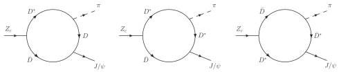
Figure 35: Example of heavy meson loops used the NREFT formalism. In the picture the decay can only happen via an intermediate pair because of the molecular nature of the itself. Since the problem is non-relativistic the propagators appearing in such loops must be the non-relativstic ones, namely:
(77) -
•
The typical velocities involved in the decay/creation of a certain particle with mass are given, in this context, by , where is the mass of the open flavor mesons appearing in the loop. Since our states are close to the threshold such velocities turn out to be small, thus allowing a the use of a non-relativistic approach and of a power counting procedure to estimate the relevance of a certain Feynman diagram[167]. In particular, every meson loop counts as while the heavy meson propagators scale as . Moreover, depending on the possible presence of derivatives in the interaction vertices, the diagram might also scale as a power of one of the external momenta, , or as an additional power of .
Since the interaction Lagrangians are non-perturbative some diagrams might be too challenging to be calculated and therefore, using this power counting technique, one can estimate the relevance of that particular process and hence determine an uncertainty related to its omission.
This formalism has been quite powerful in computing the decay width of many hadronic[166, 167, 169, 171] and radiative[167, 170] processes involving exotic mesons, assuming their internal structure to be a bound state of open flavor mesons. In particular, some attempts have been made to estimate the effective couplings appearing in Eqs. (76). The and constants have been extrapolated from the experimental value of the binding energies[170]:
| (78) |
while and have been computed from experimental widths both in the charm and bottom sectors[171, 167]:
| (79a) | ||||
| (79b) | ||||
It is interesting to note that and which indicates a large degree of spin symmetry violation. This is expected for very-near-threshold states, since small mass variations can lead to large changes in binding energies and hence in the couplings.
For the predictions made by this model about branching fractions and decay widths see Sec. 9.
Lastly, it should be mentioned that another, slightly different, NREFT has been developed in some papers[165, 159]. The main difference between such approach and the one explained above lies in how the molecular hypotesis is implemented. In particular, instead of requiring the presence of interemediate meson loops, the interpolating operator has been chosen to be explicitely . We could refer to this model as a Non-Relativistic Effective Field Theory Type II (NREFT-II).
5.2 Hadro-quarkonium
Another interpretation has been proposed[174, 175] for the resonances (namely , and ) and for the manifestly exotic . These states have always been observed in final states with a specific excitation of the charmonium spectrum, either or . In particular, for the all the observed decays contain a , while for the other exotic particles their decay products only contain a . This feature motivated a model that describes these systems as composed of a heavy charmonium “core” sorrounded by a “cloud” of light hadronic matter. Such a configuration is known as hadro-charmonium and it is an extension of a model for the binding of a or around a nucleus[176]. Note that, the distinction between a molecular states and a compact tetraquark is determined by the clustering of the constituents. For the case of the hadro-quarkonium, instead, the distinction between the heavy and light degrees of freedom is due to their size (instead of their superposition region), the light excitation being more extended that the quarkonium core.
The interaction between the central heavy quarks and the sorrounding excitation is a QCD analogous of the van der Waals force and is supposed to be strong enough to allow a bound state but also weak enough to mostly maintain the nature of the charmonium, thus explaining the absence of other excitations in the final states. Since the state is color neutral, such an interaction can be treated using a multipole expansion, in close analogy with the well-known electromagnetic case. The heavy quark pair, that from now on we will call generically as , has a chromo-electric dipole moment proportional to the chromo-electric gluon field generated by the sorrounding light excitation and this dipole will interact with the field itself, thus producing an effective Hamiltonian
| (80) |
where is the chromo-electric field generated by the sorrounding light matter and is the chromo-electric polarizability. Here and in the following we indicate with a generic element of the polarizability; in general we will have different components, , both diagonal and off-diagonal. Such a polarizability is still unknown from first principles. We can only extimate its off-diagonal values for the charmonium and bottomonium case from the and transitions[177], where one finds GeV-3 and GeV-3. The diagonal terms are usually expected to be larger that the off-diagonal ones.
Using the well-known expession for the conformal QCD anomaly in terms of the chromo-electric and chromo-magnetic fields, and
| (81) |
one can compute a lower bound[174] for the expectation value of the previous Hamiltonian (80) over a generic hadron :
| (82) |
In particular, we used the fact that and that the expectation value of must be non-negative. This can also be used to determine a condition for the presence of a bound state due to the van der Waals interection. One finds that it must be
| (83) |
with the mass of the light hadronic excitation, the reduced mass of the charmonium-light hadron system and a (model dependent) constant of order 1. From Eq. (83) one immediately notices that bound states are favoured for higher values of , i.e. for higher light hadronic excitations, but also for higher values of , which is in general considered to be larger for higher quarkonium levels. This last point would explain why three out of four of the previously mentioned exotic resonances decay into .
Using a square well ansatz for the interaction potential and a reference value GeV-3 one finds[174] that bound states might appear for GeV or for lower but higher excitations of the central core. For the case of the bottomonium, since is much smaller, one needs much higher hadronic resonances in order to allow a bound state, making an experimental analysis quite challenging. However, it is still expected for lower values of but higher excitations of the pair (in particular with a core).
It is worth noting that, so far we assumed that the nature of the heavy quarkonium does not change because of the gluonic field. However, it turns out that the interaction in Eq. (80) might cause a transition via the off-diagonal polarizability with a width of a few MeV. Therefore, the present model also predicts the , and the to decay into but with a much lower (even though still detectable) branching ratios.
Lastly, using a holographic QCD approach[175] one can show that the decays of hadroquarkonium states into open flavor mesons are suppressed by a factor in the large limit. This could explain why such final states are not observed experimentally. Recently, such a model has been applied to the and system by Voloshin and Li[178].
5.3 Hybrids
Quark model describes mesons as a quark and an antiquark which saturates color with each other. However, the QCD Lagrangian contains also the gluons, as dynamical degrees of freedom mediating strong interactions. From the point of view of the quark model, one might treat gluons as static degrees of freedom as well, belonging to the adjoint representation of the color group: since the tensor product of any number of adjoint fields always contains a singlet (), we can form hadrons made up of just gluons, the so-called glueballs. Moreover, we can add pairs in the color octet which saturates the gluon color, generating what it is usualy called a hybrid meson. The addition of a gluon allows such mesons to have quantum numbers forbidden by ordinary quark model, e.g. , and so on. In the following we present a set of models developed during the years to describe these peculiar states.
The existence of hybrid mesons in the light sector was suggested in 1976 by Jaffe and Johnson[179] in the context of the MIT bag model. Some calculation[180, 181] predict the lightest hybrid multitplet to have a mass (it is worth noticing the observation of a exotic with the exotic exactly at ). The exotic quantum numbers are due to the boundary conditions in the bag.
For the heavy quarks a spherical bag would be quite unrealistic, and thus an adiabatic bag model was introduced by Hasenfratz et al.[182]. In this model the bag was allowed to deform in the presence of a fixed source. The resulting potential is used in a Schrödinger equation to compute the mass of the states, as in usual quarkonium spectroscopy. The lightest hybrid was found at 3.9 GeV for and at 10.5 GeV for . Some recent results on adiabatic potentials in QCD string models can be found in the literature[183].
In the framework of constituent quark models, we can analogously consider constituent gluons. These models were pioneered by Horn and Mandula[184] and later developedì[185, 186, 187, 188, 189]. The gluon has a fixed orbital angular momentum relatively to the pair, usually called , and the is in a defined orbital configuration and spin configuration . The quantum numbers of such bound states are and . The lightest hybrid state within this model has and thus non-exotic quantum numbers such as are obtained using P-wave states with , while exotic states have .
The most effective pictorial representation of hybrid mesons can be achieved via the flux-tube model. Lattice QCD simulations show that two static quarks at large distances are confined by approximately cylindrical regions of color fields. More specifically, if a gauge is fixed, the magnitude of chromoelectric field has cylindrical symmetry. The flux tube models this feature by approximating the confining region between quarks with an oscillating string. If one assumes Nambu-Goto action, i.e. the action to be proportional to the area spanned by the string in coordinate space, one gets an exact potential for large values of the separation, , between the sources:
| (84) |
where is the usual string tension, and parametrizes the quantized excitation of the string. For we get a linear rising potential, which corresponds to ordinary quarkonium spectrum. Higher excitations of the string would correspond to excitations of the color field, and so can be associated to hybrids.
The previous potential is obtained as a function of the distance between the sources. In the first studies with this model an adiabatic separation of the quark and gluon degrees of freedom was carried on. Such approximation is allowed because of the large difference between the time scales of the fast dynamical response of the flux tube degrees of freedom and of the slow motion of the heavy quarks. This allows to fix the separation at some value (now considered as a parameter) and compute the eigenenergy of the system in some fixed configuration of the flux tube: , being the quantum numbers of the flux tube. This eigenenergy is then treated as an effective potential acting on the heavy quark pair. The ground state gives the ordinary meson spectrum. Hybrids are obtained for and can be studied using the excited potential . This is nothing but the QCD analogous of the time-honored Born-Oppenheimer (BO) approximation for hydrogen molecules. This approximation has been successfully used since the first estimates of the charmonium spectrum on the lattice in the infinite mass limit (static potentials). The lightest hybrid state is the one in which the string has a single orbital excitation about the axis. In initial models the adiabatic potentials were determined in the approximation of small fluctuations relatively to the axis. This approximation was later removed by Barnes, Close and Swanson[190].
Some insight on the spectrum of hybrids might be obtained from Lattice QCD simulations, which are supposed to give the most reliable predictions for absolute masses. In the heavy quark sector, when the pair is kept fixed while the gluonic degrees of freedom are allowed to be excited, the lightest charmonium hybrid was predicted[191] to have a mass of 4.2 GeV for and 10.81 GeV for . In general, in the charmonium family hybrids are predicted in the mass region around 4.3 GeV, while the bottom sector they are predicted in the region 10.7-11.0 GeV.
Unfortunately many problems have to be faced when dealing with hybrids on the lattice since, from a field theory point of view, hybrids with ordinary quantum numbers suffer the same problem than tetraquarks: they are undistinguishable from mesons. One possible solution to this difficulty is to look at the overlap (the prefactors in Eq. (64)) of those hybrid states with suitable operators. This has been recently done[133] in lattice simulations (see Figure 36) where a hybrid candidate with is found close to the mass of the resonance. Although this evidence, it is not possible to conclude that the observed state is a hybrid meson instead of, for instance, a tetraquark.

The observation of four hybrid candidates nearly degenerate with and (see the red boxes in Figure 36) is in agreement with the pattern predicted for the lightest states in the bag model[181] and in the -wave quasi-particle approach[192]. They appear at a mass scale GeV above the lightest conventional charmonia.
The picture of hybrids borrowed from Lattice QCD has been employed to try to explain some of the observed resonances[193, 194]. In particular, it has been proposed that the might indeed be an example of a hybrid composed of a pair with and a gluonic excitation with . This interpretation would explain some of the striking properties of this resonance. In particular, the smallness of the wave function at the origin, , would explain why the is observed with a small production rate in annihilation and why its decays into light hadrons are suppressed. Moreover, it is also known[195] that the decays of gluonic hybrids into a pair of -wave mesons are suppressed and hence the dominant decay (if allowed) should be into an -wave and a -wave charmed mesons. However, for the the decay into is phase space forbidden and the decay into is suppressed by a -wave coupling. The only drawback of this interpretation was that the decays into charmonium plus light hadrons were also expected to be suppressed and this is in striking contrast with the observed large branching fraction for the channel.
This problem found a solution with the discovery of the . It has, in fact, been hypotesized that this particle might be a different example of hybrid, a so-called tetraquark hybrid. The main idea is that the excited gluon can be replaced with a pair of light quarks belonging to the adjoint, , representation of the color group. In this context, the would be made out of a pair with and a pair with , this last assignement being motivated by the analogy with the gluonic hybrid, where the lowest energy excitation has these quantum numbers. If this idea were true, the decay would be explained as a transition of the gluon within the hybrid into a by pion emission, thus explaining the observed branching fraction.
A similar interpratation has also been given for the and states, even though in this case their closeness to the would also provide them with a strong molecular component.
As previously anticipated, the spectrum for gluonic and tetraquark hybrids can be computed under the BO approximation. To do that, one considers the pair to simply be a fixed source of color field, with a separation and solve for the eigenenergy of the gluonic (tetraquark) excitation. Once this is done this energy is taken as the effective potential suffered by the pair. Such a potential is given by Eq. (84) for large value of and by a Coulomb-like expression for small :
| (85) |
where is the strong coupling constant evaluated at a scale and is the so-called gluelump, i.e. an additive term that depends on the quantum numbers of the considered gluonic field (see for example Marsh and Lewis[196]). The parameters related to the previous potential can be fitted from lattice QCD results by Morningstar et al.[197]. Once this is done one can solve the Scrödinger equation for the pair with this potential:
| (86) |
where is the orbital angular momentum of the pair computed for certain quantum numbers and for a separation . is the usual radial wave function. We will not go into the details of the this calculation since it is rather involved and does not add anything interesting to our discussion. In Figure 37 we report the spectrum for the excited gluonic hybrid obtained from this calculation in the charm and bottom sectors. For the charmonium case the lowest energy level is estimated to be MeV, while for the bottomonium case it is MeV.
In the tetraquark hybrid case we have no insight on the actual shape of the potential generated by the two quark-antiquark in the adjoint representation. It has been proposed[193, 194] to assume a similar behavior as in the gluonic case. From this assumption and from a certain number of input values one can try again to derive a spectrum for this second kind of hybrids, and some generic selection rules. However, it is worth noticing that the hybrid potential computed on the lattice relies on quenched simulations (i.e. without dynamical fermions), or on simulatios with unphysical light quarks masses (typically ). The excited level corresponing to the hybrid state becomes more and more noisy, and the potential becomes more and more difficult to extract when approaching the physical point. In particular, at the physical pion mass the potential could be rather different from the present computations.
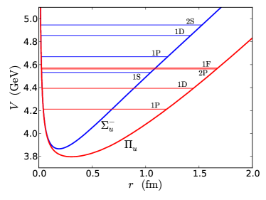

While the masses of hybrid mesons are computable in all the models listed above, and in particular in Lattice QCD, the decay dynamics is more difficult to study.
The only model which offers a description of the decay dynamics is again the flux-tube model. In fact, in this picture, the decay occurs when the flux-tube breaks at any point along its length, producing in the process a pair in a relative state. Again this is just the well-know Lund model for ordinary mesons. The distance from the axis at which the light pair is created is controlled by the transverse distribution of the flux-tube. This distribution varies when going from the non-excited flux-tube to the first excited flux-tube configuration. Exploiting the empirical success of this model in describing the ordinary mesons decay dynamics, Close and Page[198] derived the decay pattern for hybrids. They found that in a two-meson decay the unit of orbital angular momentum of the incoming hybrid around the axis is exactly absorbed by the component of the angular momentum of one of the two outgoing mesons along this axis. They treated explicitly the light flavor case[198], but a generalization to hybrid charmonia is straightforward. The final state should be in this case , where indicates -meson which are formed from P-wave () pairs. However, since the masses predicted in the flux-tube model are about , i.e. below the threshold, it is possible that this decay is kinematically forbidden giving a rather narrow resonance decaying in charmonium and light hadrons. These modes offer a clear experimental signature and furthermore should have large branching fractions if the total width is sufficiently small.
5.4 Alternative explanations
It should be mentioned that there are other interpretations about the nature of the states. In particular, it is worth spending a few words about cusp effect. Some of these exotic states, in fact, lie slightly above their open flavor threshold. This suggested to some authors[82, 151, 199, 200] that the experimental signals seen by the various collaborations might not be due to actual particles but to a dynamical effect. Cusps, in fact, can occur in amplitudes at threshold and these can manifest themselves as bumps in the cross sections right above the threshold. The proximity of many of these states to their open flavor threshold suggested to these authors that the cusp option might be taken seriously. Such possibility has been studied for the [82, 199], for the [82, 201] and most recently for the and [200]. This interpretation has been recently challenged by Hanhart et al.[202].
Finally, some authors try to describe the exotic neutral candidates like as ordinary charmonia whose properties are deformed by the thresholds, see for example the Unquenched Quark Model by Ferretti et al.[203].
Sec. 6 The prompt production of
In this section we report a brief summary of an old controversy about the molecular interpretation of the . The main drawback of this picture, in fact, lies in the unexpectedly high production cross section measured at Tevatron and LHC that, for many years, has been seen as the definitive proof of the inconsistency of the molecular interpretation.
The description of the in terms of a very loosely bound meson molecule is often compared to the well-known case of the deuteron, both being bound by strong interactions and having very small binding energies[156, 84], MeV and MeV.
The deuteron can be described by means of the phenomenological coalescence model[204, 205], according to which a neutron and a proton will bind together if they are produced with a relative momentum smaller than a coalescence momentum, MeV. Because of the close analogy between the deuteron and the we might wonder if a similar approach could be valid for the latter as well. In particular, in both cases, one might expect to have a very small yield of such loosely bound molecules in high energy hadron collisions, since their component will naturally tend to be produced with a very high relative momentum, thus preventing the system from binding.
The validity of this qualitative expectation and of the coalescence model for the case of the anti-deuteron has been successfully tested[206] using the well-known Monte Carlo (MC) generator HERWIG[207]. In particular this tool has been used to evaluate the number of pairs produced with small relative momentum ( MeV) in collisions at TeV in the interval GeV GeV. The results obtained have been compared to the preliminary data on anti-deuteron production from the ALICE experiment at LHC[208]. The results of this analysis are reported in Figure 38. By anti-deuteron events we mean the number of pairs produced with a momentum smaller than MeV. As one can see in Figure 38, the MC simulation describes the experimental data, thus providing a proof of the validity of the coalescence model.
In Figure 38 the authors extrapolated the transverse momentum range up to GeV. In order to increase the statistics enough, they allowed the relative momentum between the pair to be up to MeV since the simulation showed that the shape of the distribution was totally uncorrelated with 131313The dependence coming from phase space is reabsorbed in the normalization factor used to tune the distributions on the experimental data.. This rough estimate shows how the production cross section for anti-deuteron might turn out to be really small at high , in agreement to the intuitive picture mentioned before. There is, in fact, a close relation between the of the pair and their relative momentum, as it turns out that it can be written as , being the relative angle between and and with , with being the angle from the beam axis. Hence, since the kinematical cuts used in the simulations give , for a generic , high is equivalent to high relative momentum. Data from ALICE up to GeV in anti-deuteron production might be available and would be highly discriminative for the molecular picture of the .
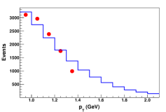
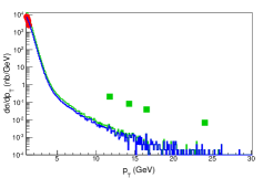
It is exactly this qualitative expectation that casted many doubts on the interpretation of the in terms of loosely bound meson molecule. Such particle was, in fact, observed both by CDF [27] and CMS [93] with a very large prompt – i.e. directly produced at the collision vertex – production cross section, nb. This experimental fact seems at odds with the previous conclusion about the deuteron and, more in general, about hadronic molecules with very small binding energy.
In particular, it is possible to estimate an upper bound for the production cross section of the as follows[114]:
| (87) |
where is the relative momentum between the two mesons and is the domain where the two-body wave function for the molecular is significantly different from zero.
Such an upper bound can be estimated by simply counting the number of 141414Here and in what follows we will omit the charge conjugate system, , for simplicity. produced with a relative momentum lower than a certain value. This has been done[114], again, using HERWIG and PYTHIA[209] (see Figure 39), taking to be a ball or radius MeV, on the basis of a naïve gaussian shape for the two-body wave function of the . The result of the MC simulation was a production cross section of nb for HERWIG and nb for PYTHIA, which are both smaller than the experimental value by more than two orders of magnitude. This is also confirmed by comparing the expected cross section at high for the anti-deuteron with the CMS data for the – see Figure 38. In fact, if we assume that the spin-interactions are second order effects, the yields for the anti-deuteron and for the should be similar. In Figure 38 the simulated cross section is again two orders of magnitude smaller that the experimental one. This seemed to be the definitive proof of the inconsistency of the molecular interpretation with the experimental data.
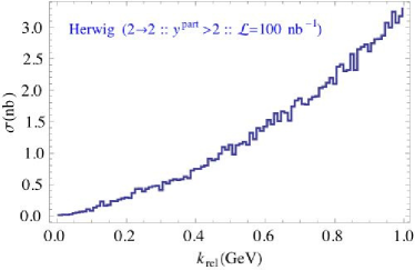
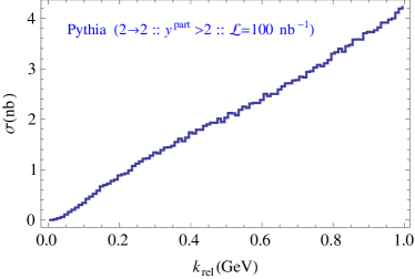
However, the previous approach was later criticised and it was shown[210] that the theoretical and experimental cross sections might be matched resorting to Final State Interactions (FSI)[211]. The possible presence of FSI, in fact, casts doubts on the applicability of the simple coalescence picture to the case of the , since the two components of the molecule could be bound by final state rescattering even when their relative momentum is large. In particular, the Migdal-Watson theory would change the previous results in two different ways:
-
1.
The cross section for the production of the should be modified to
(88) where is the upper bound evaluated in (87) and is the typical range of the interaction between the components;
-
2.
Instead of being the inverse of the spread of the spatial wave function, the maximum value for the relative momentum should be given by the inverse of the range of the interaction, , with .
By setting MeV one can increase the theoretical cross section up to nb, which is in agreement with the experimental value.
However, this approach has some flaws[212]: it can be shown that the use of Eq. (88) should enhance the occurrence of a new hypothetical molecule, the , which otherwise would be suppressed, as one could infer by looking at data on production at Tevatron[213]. In fact, the theoretical production cross section for this would be nb and should be detected by the CDF experiment. No hint for such a particle has been found. Furthermore, the applicability of the Migdal-Watson theorem requires that, (i) the two final particles should be in an -wave state and (ii) they should be free to interact with each other up to relative distances comparable to the interaction range. First of all, the inclusion of relative momenta up to MeV means to include relative orbital angular momenta up to , thus violating the hypothesis (i). Moreover, using again the MC softwares HERWIG and PYTHIA, one can show[212] that in high energy collisions, such as those occurring at Tevatron and LHC, there are on average more hadrons having a relative momentum with respect to one of the two components smaller that MeV, thus violating the hypothesis (ii) – see Figure 40. Lastly, it seems really odd that the presence of FSI plays such an important role in the case of the but not in the case of the deuteron which, as we showed, is already very well described by a simple coalescence picture.
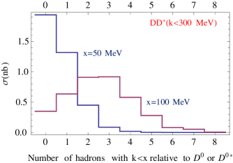
Even though the presence of other hadrons (mainly pions) sorrounding the system does not allow the use of FSI, it might still play an important role in explaining the unnaturally high prompt production of the .
It has been proposed[158] that the possible elastic scattering of these “comoving” pions with one of the components of the molecule might decrease their relative momentum, hence increasing the number of would-be molecules. This possibility can be understood intuitively referring to the distribution of meson pairs as a function of as reported in Figure 39. The idea is that the interaction might push the pair both to higher and to lower values of . However, since the majority of would-be molecules are produced with high relative momenta, even if a small fraction of them would be pushed to smaller momenta, that could cause a feed-down of pairs towards the lower bins of the distribution, where the candidates live. For a pictorial representation of the considered rescattering mechanism see Figure 41.

It is worth noting that, if we assume the initial total energy of the pair to be positive, the decrease in due to the elastic scattering may bring it to negative values, hence assuring the binding of the molecule. Therefore, in this model the would be a genuine, negative energy bound state, whose lifetime would be entirely regulated by the lifetime of its shorter lived component, the . Hence, this mechanism also predicts a narrow width, keV, in accordance with the experiments.
Once again, this idea has been tested[206, 158] with the already mentioned MC algorithms. In particular, the recipe used to implement the interaction with the pions is as follows: first of all the 10 most coplanar pions to the plane are selected, then the pion which will interact with (say the ) is randomly chosen and lasty the most parallel pion to the non-interacting meson (say the ) is selected. One expects this configuration to be the most effective in physical events. Moreover, in order to prevent that mesons belonging to different jets (separeted in coordinate space) would get closer by the scattering with a hard pion, one also requires . The interaction in the centre of mass is given by
| (89a) | ||||
| (89b) | ||||
with and [172].
First of all, it has been checked[206] that this new mechanism does not spoil the high energy behavior of the relevant meson distribution, as shown in Figure 42. It was actually showed that the inclusion of one elastic scattering improves the agreement of the simulation with the experimental data from CDF– see Table 6. This is a strong hint of the fact that this mechanism actually takes place in real physical events and should hence be considered when studying final hadronic distributions.
Fit values referring to the distributions in Figure 42. -factor /DOF (blue) 1.35 45/11 (red) 3.46 24/11

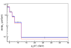
As one can see from Figure 43 the proposed mechanism is actually effective in feeding down the lower MeV bin, the one containing the would-be molecules. It is also possible to estimate how many of these interactions may take place. In particular, considering a model where all the produced hadrons are flying away from each other on the surface of a sphere – see again Fig. 49 – and taking into account the range of the interaction, one finds[158] that the simulations suggest an average of 3 scatterings per event. These consecutive interactions can be reproduced by implementing a Markov chain[158]. In Table 6 we report the values of the integrated cross section for the production of the varying both the number of interacting pions and the maximum allowed for the pair.
Effect of multiple scatterings in production cross section. indicates the integration region . 50 MeV 300 MeV 450 MeV 0.06 nb 6 nb 16 nb 0.06 nb 8 nb 22 nb 0.9 nb 15 nb 37 nb
As one can see, if one trusts the coalescence model for the – as the data on deuteron strongly suggest – and hence consider MeV, not even the elastic scattering with three consecutive pions is able to raise the production cross section up to the experimental one ( nb). Moreover, if one considers the (questionable) use of FSI[205, 210] as explained previously, then it should be MeV. With this integration region, the simulations produce a cross section after the interaction with one pion – and after a rescaling needed to take into account the different normalization factors between the two works[205, 206]– that is equal to nb, larger than the experimental one.
To summarise, the experimental value of the prompt production cross section of the casted serious doubts on its possible interpretation in terms of a molecule. According to the expectations following from the phenomenological coalescence model – that correctly describes the well-known deuteron – the production of such a weakly bound state should be strongly suppressed in high energy collisions. Even though many ideas and models have been proposed during the years none of them has successfully reconciled the theoretical expectations with the experimental results.
Sec. 7 Tetraquarks
The previously described problem seemed a compelling evidence of the necessity for a new kind of interpretation for these exotic mesons. It has been proposed[214] that these states might actually have a compact (point-like) four-quark structure – the so-called tetraquark. In this section we introduce this model starting from its consequences regarding the production of mesons in high energy collisions, so that a more direct comparison could be done with the previous section. One of the simplest and more economic ways (in terms of new states predicted) of forming tetraquarks is the diquark-antidiquark realisation based on the binding of a diquark and an antidiquark . This was originally proposed by Jaffe and Wilczek to explain pentaquark baryons[215] (diquark-antidiquark-quark). In general tetraquark bound states have been proposed a long time ago[216, 217, 218] to understand the nature of the light scalar mesons and . An interpretation of light scalar mesons in terms of diquark-antidiquark states was instead proposed for the first time by Maiani et al.[7, 219] following the revitalization of interest on the meson (reappeared in heavy-light meson decays[220]) and contextually with an interesting reanalysis of scattering[221].
Some aspect of the tetraquark models have been inspired by dibaryons[222, 223], in particular the feasibility of isospin violation[224]. Different extensions of the constituent quark models for the tetraquark spectroscopy have been explored by Valcarce et al.[225, 226, 227, 228, 229].
As we will show in the next sections, assuming a constituent quark model with color-spin interaction it is possible to study the spectroscopy of these states, in which the and states discovered so far can be nicely accommodated. The main problem with this picture is that it also predicts other states which did not (yet?) show up in experimental researches. A possible solution to this problem is also presented.
7.1 Tetraquark production
From the studies on loosely bound molecule production at hadron colliders we are led to consider that multiquark hadrons should rather be initiated by the formation of compact quark clusters. The seed of a heavy-light tetraquark state state could be described by
| (90) |
where by and we represent the heavy and light quarks respectively. In our scheme, the two-meson states will tend to fly apart, as strong Van der Waals-like forces between their meson components are not sufficient to produce bound states like or – depending on the spin and orbital quantum numbers of the original four-quark system. In this sense such states are in a “open channel” continuum.
Most authors are convinced instead that some hadron molecule shallow potentials could allow for at least a single discrete level with almost zero energy . Small binding energies in quantum field theory are possible and, if is the strong coupling, say in the interaction, one can connect to by
| (91) |
where is the reduced mass of the system (in this formula we are treating and as if they were spinless particles. Accounting for the spin is simple and does not change our qualitative conclusions). This formula is obtained by resonance scattering theory at low energies supposing that there is a pole term associated with the virtual production of particle in the scattering amplitude
| (92) |
and supposing that , the barycentric energy after subtraction of rest energy, is, like , a small quantity. We replace .
Thus, if were indeed small enough, formula (91) would hold and, including spin and using the coupling as deduced in[230], one would get
| (93) |
from (91).
However in the prompt production of at large hadron colliders, is very far from being small. The fact that the observed prompt production cross section at LHC is so much larger than expectations, as commented at length in previous sections, suggests then that the is not a loosely bound state of , and the rough agreement (93) simply occurs outside of the kinematic conditions of production.
These kind of problems do not exist in the diquark-antidiquark picture for this particle would be kept together by color interactions, the unknown being the effectiveness of the color force at producing diquarks. The diquark-antidiquark belongs to a “closed” channel. The relative size of coefficients in (90) is unknown.
We might formulate different hypotheses: are all of the same order. In this case we should be observing the entire spectrum of diquark-antidiquark states which can be predicted using the color-spin Hamiltonian (see below). In a previous work[214], the Hamiltonian of the diquark-antidiquark model was supposed to contain both spin-spin interaction between quarks within each diquark and quarks in the two different diquarks. The resulting spectrum predicts a rich structure of states with some evident mismatches with the experimental findings.
A ‘type-II’ version of the diquark-antidiquark model, with spin couplings suppressed between different diquarks, allows a remarkable description of the sector of charged tetraquarks as the , , and a good picture of the entire sector (see next few sections). Some typical problems of the diquark-antidiquark model persist in the type-II model. For example the should have charged partners and an hyperfine splitting between two neutral levels, to account for isospin violations[214].
To solve this kind of difficulties we might formulate a different hypothesis for the hierarchy among coefficients. We might indeed assume that,
| (94) |
Such an assumption means that, in general, diquark-antidiquark states are less likely to be formed in hadronization but a resonance could emerge as a result of the coupling between open and closed channels. This hypothesis introduces a selection rule in the diquark-antidiquark spectrum: especially those levels which are close enough to open channel thresholds (resonance conditions) are observed as physical resonances.
More specifically, the diquark-antidiquark closed channel provides an effective attraction in the open channel which might lead to produce a resonance. This phenomenon is effective if the energy level , corresponding to the closed channel state , happens to be very close to one, or both, as in the -particle case, of the open channel thresholds (located, in the case of the , at or ).
Strong interactions provide the discrete spectrum for diquark-antidiquark states, however those levels correspond most likely to physical states once the closed channel is hybridized with the open one, i.e. the difference in energy, or detuning parameter , is small enough. When this energy matching condition between the total energy in the open channel and the energy level in the closed channel takes place, the two hadrons in one open channel can undergo an elastic scattering, altered by the presence of the near closed channel level. The two hadrons in an open channel can scatter to the intermediate state in the closed channel, which subsequently decays into two particles in one of the open channels.
The contribution to the scattering length due to this phenomenon is of the form
| (95) |
where couples the open and closed channels; the discrete levels of the closed channel are labeled by . This sum is dominated by the term which minimizes the denominator , i.e. the one with the smallest detuning. The width of the resulting resonance is naturally proportional to the detuning for phase space arguments.
Since the is the narrowest among all mesons, it must have , which means the highest possible hybridization between channels given the (unknown) inter-channel interaction Hamiltonian .
The open channel level is found to be at a mass above the diquark-antidiquark level, by about 8 MeV. Coupling between channels gives rise to a repulsive interaction if the energy of the scattering particles is larger than that of the bound state (and an attractive one if it is smaller). For this reason we might conclude that the neutral particle has no content in its wavefunction explaining the well-known isospin breaking pattern in decays.
The diquark-antidiquark levels (the charged partner of the ), might also fall below and thresholds by about MeV, which could be enough for inhibiting the resonance phenomenon described. This might be the reason why the particles, although present in the diquark-antidiquark spectrum, are more difficult to be produced.
The open channel level is also perfectly matching the closed channel one for the . However because of the large width, the modification in the scattering length (95) is much less effective if compared to the open charm threshold: the sum in (95) has to be smeared with an integral convoluting the Breit-Wigner. Therefore we would expect that the particles are less likely to be formed or they could simply be too broad to be observed. Some examples are shown in Table 7.1.
The mechanism here described is known in nuclear and atomic physics as the Feshbach resonance formation[160].
Exotic states in term of Feshbach resonances. The width is related to the detuning by . An exception is given by the , whose width is forced to be larger than its constituent width, i.e. . State Open channel () () ()
Recently two charged resonances have been confirmed to a high level of precision. The and the . These are genuine tetraquark states. We need to recall that the prediction of charged states of this kind was exclusively formulated in the context of compact tetraquark states[214].
In particular, when the first hint of a charged tetraquark was provided by the Belle collaboration in the channel, back in 2007, it was observed that another state at 3880 MeV (i.e. lighter by the mass difference) was expected in the tetraquark model[231] with the same quantum numbers (the former being the radial excitation of the latter). The lower state was expected to decay into or . A charged with decaying into was discovered by BES III and Belle in 2013[40]. It was also shown that BES III and Belle data might be compatible with the presence of another peak about 100 MeV below that of the [232]. That was also predicted by the tetraquark model.
The tetraquark model in its first diquark-antidiquark version[214, 232] predicts one more level, at a mass of MeV (these mass values are locked to the input mass value of the ). We might predict that no resonance will be found at this level because there are no open channels nearby to make the Feshbach mechanism possible. The is instead made possible by the presence of the open channel. The expected width, driven by the , is expected to be as large as MeV, to be compared with the MeV observed.
The tetraquark model in its ‘type-II’ version has no MeV, but a level perfectly compatible with the observed by the BES III Collaboration[43], which is also compatible with a Feshbach generated state. A isosinglet resonance could be due to the vicinity of the open channel, with a narrower width of about MeV. For a tetraquark interpretation of the states in the bottomonium sector, see Ali et al.[233, 234, 235, 236].
These considerations about the interplay between a closed (diquark-antidiquark) and open channel (molecular thresholds) are to be considered in a preliminary stage and possibly object of future developments. In the following we will focus instead on the description of the diquark-antidiquark closed channel listing its states by quantum numbers and showing how to estimate expected masses (the position of levels).
We believe that recent experimental findings are clearly spelling in favor of tetraquark particles and the diquark-antidiquark model apparently has many features matching very well the present phenomenology. The Feshbach mechanism here sketched might be a viable way for implementing those selection rules still missing in the tetraquark Hamiltonian approach to be described below.
7.2 Diquarks
One-gluon interaction in the -channel between two quarks in the representation (antiquarks ) involves a (tensor) product of color charges which can be expressed as the direct sum of diagonal blocks with the dimensions of the irreducible representations in . According to the general rule
| (96) |
we only need the Casimir values and to appreciate that one-gluon exchange generates a quark-quark attraction in the channel () which is just half of that in the quark-antiquark singlet channel (). Even if one-gluon-exchange interaction is a primitive model of low energy strong interactions, correlating it with indications from lattice computations[237] on diquarks gives reasonable support to the possibility of diquark-antidiquark hadrons.
Diquarks carry the same color charge of antiquarks. The opposite for antiquark-antiquark pairs. We represent a spin zero diquark with the bispinor notation
| (97) |
where , and are color indices. In the quadrispinor notation we would have written , where indicates the charge conjugated spinor. In the next sections color index will be left implicit. Relaying on spin-flavor symmetry of heavy-light mesons, a spin-1 heavy-light diquark could equally be formed
| (98) |
The color-spin Hamiltonian is, e.g. Eq. (4.3) in Jaffe’s report[238]
| (99) |
Here we will discuss the color interaction only, leaving the spin to the next sections. We introduce the (normalized) color singlet/octet states using the following notation which turns out to be rather practical for calculations:
| (100a) | |||
| (100b) | |||
where by , for example, we mean using latin letters for color indices.
With the notation we mean an overall color singlet state of a diquark-antidiquark pair:
| (101) |
Using the relation
| (102) |
one obtains
| (103) |
i.e. the octet-octet component has twice the probability of the singlet-singlet one. The previous state can itself be normalized in the following way (multiply by )
| (104) |
and use the matrices.
Let us represent states of the fundamental representation with the symbol whereas those of the anti-fundamental are . Then we have
| (105a) | |||
| (105b) | |||
i.e. one is the opposite of the transpose (complex-conjugate) of the other.
From the latter equation we get
| (106) |
Consider a generic state
| (107) |
then
| (108) |
We thus conclude that (multiply the latter by and then rename )
| (109) |
whereas
| (110) |
If, for example, we consider the action of the Hamiltonian term , according to (109,110) we have to replace
| (111) |
Similarly if we start with some , where is some combination of ’s, we have to replace
| (112) |
With this rules we can compute the action of on a diquark state defined in (104)
| (113) |
and thus
| (114) |
where we have used
| (115) |
and
| (116a) | |||
| (116b) | |||
As for the color, taking matrix elements on diquark-antidiquark color-neutral states amounts to redefine the chromomagnetic couplings by some numerical factor: when the and terms are considered. Actually we assume that the dominant couplings in the Hamiltonian are and , i.e., intra-diquark interactions. We take them to be equal 151515 If extra-diquark couplings were considered we could determine them, e.g. , from the masses of standard mesons observing that (117) . .
7.3 Diquark-antidiquark States with
The following discussion is mostly based on a recent paper[239] where, as anticipated, a ‘type-II’ tetraquark model is introduced.
7.3.1 The tetraquark
Consider a tetraquark made up of two quarks and two light quarks, with the same flavor: a neutral component. Using explicit spin indices we write them in the order:
| (118) |
Assume that the pair has spin 1 whereas the antidiquark has spin 0. Then the spin indices are saturated by the operators
| (119) |
for the pair and
| (120) |
for , where repeated indices are summed. We might write the operators as
| (121) |
and recall that
| (122) |
Let us consider the first term in (122) and plug it into (121)
| (123) |
therefore forcing the pair to be spin 1 and to be spin 0. Strong interactions are not supposed to change the heavy spin, thus we may assume that the color octet components of the will maintain spin 1 configuration whereas light quarks can rearrange their spins, when in the octet configuration (twice as probable as the singlet one; see Eq. (103)), in such a way to fulfill decay quantum number conservation laws.
Consider now the second term in (122) and plug it into (121) to obtain
| (124) |
Here we use that
| (125) |
Consider the first term in (125) and plug it back into (124) to obtain
| (126) |
This term forces the pair to be spin 0 and the pair to be spin 1. Inserting the second term on the right-hand-side of (125) into (124) we have instead
| (127) |
forcing both pairs to be spin 1 and the tetraquark to be spin 1.
Here we may introduce the definitions:
| (128a) | |||||
| (128b) | |||||
| (128c) | |||||
With the symbol we either mean a diquark in the order or or a quark-antiquark pair in the order or . The ordering is relevant. The normalizations in (128a,128b,128c) are obtained using that , where . Therefore, taking for example (128c), we have (summing over repeated indices)
| (129) |
therefore we choose the normalization .
According to the quark ordering in (118), the spin 0 component will be
| (130) |
whereas in the definition of a heavy light diquark state, see (128a), might also be (heavy quark on the left). On the other hand:
| (131) |
This is not the case if we consider :
| (132) |
Therefore, putting together (123,126,127), and keeping in mind that the following states are defined up to an overall minus sign (depending on the initial definition of diquark), we obtain
| (133) |
On the other hand, if we restart from (118) but with taken with spin 0 and with spin 1 we get
| (134) |
Subtracting (134) from (133) we therefore obtain the result
| (135) |
Since diquarks are defined to be positive parity states, overall we have and . This diquark-antidiquark arrangement is a natural candidate to describe the , which is a resonance decaying into , compatibly with the assignment – especially for what concerns the heavy spin.
If we had started in (118) with the ordering
| (136) |
then in place of (133) and (134) (exchange labels ) we would have obtained:
| (137a) | |||||
| (137b) | |||||
or
| (138) |
which is compatible with the decay mode of the . Anyway, light quark spins in or configurations might rearrange also to allow or decays although the latter is phase space forbidden and the former is simply forbidden by quantum numbers.
7.3.2 The tetraquark
The orthogonal combination to the lhs of (135) might be formed, namely:
| (139) |
This has and for the neutral component (if an isospin triplet is to be considered, the parity has to be ). Using (133) and (134) we obtain
| (140) |
The state in the quark-antiquark basis has since . In the quark-antiquark basis there is another state with , orthogonal to
| (141) |
From what just found (reversing the reasoning leading to Eq. (135)) this state, in the diquark-antidiquark basis, corresponds to
| (142) |
which is indeed a state. Exchanging the coordinates, spins and charges of two fermions/bosons having each spin , the total wavefunction has to be completely antisymmetric/symmetric under this exchange:
| (143) |
which in the case of (142) is
| (144) |
giving . The case of is different as the charge conjugation operator concerns the distinct and pairs.
Linear combinations of and which diagonalize the spin-spin Hamiltonian can be identified with and .
7.3.3 Scalar and Tensor states
The diquark-antidiquark model also allows for states with . We have two states and a tensor one:
| (147a) | |||||
| (147b) | |||||
| (147c) | |||||
which are all charge-conjugation even. We use the definitions
| (148a) | |||||
| (148b) | |||||
| (148c) | |||||
where indices are symmetrized; in the latter equation (a factor of has to be included in the symmetrization) and the trace is subtracted.
The normalization in (148b) is chosen in such a way that the square of
| (149) |
is equal to 1:
| (150) |
thus . In the case we have for the first term in parentheses (148c):
| (151) |
whereas the second term squared gives . The crossed term is so that .
Now we recall that
| (152) |
and observe that (148a) may be written as
| (153) |
which contains . Substituting the completeness relation (152) in place of in the latter expression we get
| (154) |
where the minus sign arises to preserve the ordering (instead of – see discussion before Eq. (130)) whereas the factor of is introduced in agreement with (148b).
Consider now (148b) which might be written as (because of (132))
| (155) |
and make use of the relation
| (156) |
which immediately leads to
| (157) |
up to an inessential overall sign. Considering the conservation of the heavy quark spin, we see that both scalar states found might decay into a spin 0 or spin 1 charmonium.
Finally consider (148c):
| (158) |
With the usual Fierz transformation, we have
| (159) |
and symmetrizing and using the Pauli matrices properties, we get
| (160) |
The term proportional to in Eq. (148c) after a Fierz transformation cancels the singlet terms in Eq. (160). We conclude that
| (161) |
We summarize these results in Table 7.3.3.
We list the states obtained together with possible assignments and decay modes. We refer here to the neutral components. A parity may be assigned to the particles. Searches by BABAR and Belle still exclude a assignment for the , however a mixed and seems possible as well as very broad charged partners of . Resonance Assig. Decays + light mesons + light mesons , + light mesons
7.4 Spectrum of states
We assume that the spin-spin interactions within the diquark shells are dominant with respect to quark-antiquark interactions. Then the Hamiltonian would be
| (162) |
Consider for example
| (163) |
where summation over is understood. The matrix works on whereas on . Considering that
| (164) |
where we have used . Considering also the antidiquark contribution one readly finds
| (165) |
thus
| (166) |
and
| (167) |
Similarly:
| (168a) | ||||
| (168b) | ||||
We can also determine
| (169a) | |||||
| (169b) | |||||
The Hamiltonian (162) is diagonal in the diquark-antidiquark basis formed by the states of Table 7.3.3:
| (170) |
, . This requires to be lighter than . Similarly:
| (171a) | |||||
| (171b) | |||||
so that we conclude that and are degenerate in first approximation their masses being twice the diquark mass plus the same spin-spin interaction correction
| (172) |
The (and the hypothetical tensor state) is instead heavier by a gap of :
| (173) |
As for the scalar case, from (169a,169b) we have
| (174a) | |||||
| (174b) | |||||
showing what was anticipated in Table 7.3.3, i.e. that .
Considering an average mass value between and we can solve finding MeV and MeV, indicating that MeV and MeV – for a pictorial representation see Figure 44.
In this scheme we propose that the newly discovered is the first radial excitation of the as .

7.5 Diquark-antidiquark States with
Tetraquarks with can be obtained with odd values of the angular momentum; here we set and select charge-conjugation odd states.
In the diquark-antidiquark basis of we have:
| (175a) | |||
| (175b) | |||
| (175c) | |||
| (175d) | |||
Aside from orbital angular momentum considerations we can still make use of Table 7.3.3 to read the (conserved) spin; see Table 7.5. Observe that the spin structure of and in (135) is exactly the same. The mass difference between and might entirely be attributed to the orbital excitation of . The fact that and have the same spin structure also suggests that radiative transitions with and might occur:
| (176) |
as confirmed by the conspicuous radiative decay mode[70]
| (177) |
Other transitions are reported in Table 7.5.
The relative probability of having spin 1 versus spin 0 in the pair as read by Table 7.3.3. Observe that is predicted to decay preferably in where . The states and correspond either to the broad structure in the channel as described by Yuan[63, 64] or the narrow one. In this respects the mass ordering can be reversed becoming lighter than if the assignement is taken. Radiative decays are suggested by conservation of the heavy quark spin – see Table 7.3.3. State Assignment Radiative Decay 3:1 1:0 1:3 1:0
The experimentally well established and are interpreted as radial excitations of (see Table 7.5) and . We may note correspondences as and . For the identification of the state as the structures seen in , see Faccini et al.[240].
As for the , decaying predominantly into , we recall that there is also the possibility of its assignment to a tetraquark degenerate with [116].
7.6 Spectrum of states
We use the same Hamiltonian form (162) with the addition of a spin-orbit and a purely orbital term – here the chromomagnetic coupling is taken to be different from used in (162). We have then:
| (178) |
in such a way that energy increases for increasing and , provided are positive; indeed and the masses of states will be given by
| (179) |
where are the total spins of diquark and antidiquark. The latter equation can be simplified to
| (180) |
with
| (181) |
From Eq. (180), the mass of the state in (175a) is given by
| (182) |
for , therefore implying , and . The state in (175b) has or , thus – considering that contains we can determine the mass gap between and :
| (183) |
requiring . The state has both spins but so that
| (184) |
which can take either sign depending on difference; and have in principle similar size. Finally has both spins and so that
| (185) |
requiring . So the mass ordering is or from lighter to heavier. Using the assignments in Table 7.5 (chosing ), from (183,184) we obtain:
| (186a) | |||
| (186b) | |||
in units of MeV, giving
| (187) |
If we had chosen we would have obtained
| (188) |
The values found for have to be compared with the value of MeV obtained studying the spectrum of states. Both choices are reasonably consistent with it also in consideration of the simplicity of the model described. With respect to the results found in the original paper[214], we can conclude that diquarks in tetraquarks are expected to behave in a different way from diquarks in baryons: in the latter case the coupling is found to be rather smaller MeV.
As a crosscheck, observe that from (185) we get a reasonable agreement with the assigned mass of :
| (189) |
7.7 Amplitudes in the compact tetraquark model
Although one can use the phenomenological constituent quark model to predict the mass spectrum of the tetraquark states, our lack of knowledge on the actual internal structure of such particles is still almost total. The exact solution of this problem would require to solve a four-body problem, having at least a hint on the nature of the strong potential binding the four constituents. This implies that, until now, we have no methods to compute scattering amplitudes for these states from first principles.
The typical approach is to gain as much information as possible from available experimental data. In particular, one usually takes into account the kinematics of a decay parameterizing the matrix elements in terms of an unknown effective strong coupling times the most general Lorentz-invariant combination of polarization and momenta with the right behaviour under parity and charge conjugation. The effective strong coupling is typically fitted from experimental data when available or, otherwise, it can be estimated by dimensional analysis and under the assumption for it to be of “natural size”. In the latter case one can clearly just give an order of magnitude estimate of the amplitude considered.
To be more definite let us make a classic example: the decay . This is a strong decay and its matrix element can be parametrized in the following way:
| (190) |
where is the effective coupling and and are the polarization vectors of the and of the respectively. This decay already conserves total angular momentum and parity when happening in -wave. The next parity-conserving contribution to the matrix element would be the -wave one, which however must be proportional to a momentum squared and hence is suppressed by the small -value for the reaction. Therefore, we want a Lorentz-invariant combination of the available quantities with no momentum dependence. Such combination is clearly just the product of the polarization. The effective coupling can be fitted from the known experimental width for the process considered, obtaining[232] GeV.
Very recently, an interesting paper by Brodsky et al.[242] proposed a model for the internal dynamics of a tetraquark to compute the effective coupling of the exotic states to quarkonia (). The idea is that after the diquark-antidiquark pair is created, it tends to convert all its kinetic energy into potential energy of the color flux tube until it comes to rest at a relative distance . Such distance must satisfy , where is the mass of the exotic particle, is the constituent diquark mass and is the spinless Cornell potential. This essentially means that the mass difference between the exotic meson and its diquark-antidiquark constituents is given by the potential energy at . Once is computed, one can evaluate the quarkonium component of the diquark-antidiquark wave function, i.e. the overlap , being a generic quarkonium, a light hadron and the diquark-antidiquark pair. The larger is this component at the more probable the decay of the exotic state into that particular quarkonium – see Figure 45. In other words, the effective coupling can be taken to be proportional to .

7.7.1 Brief review on QCD sum rules
Another technique used to compute the mass, widths and coupling constants for these exotic states is to employ the well-known QCD Sum Rules (QCDSR)[243]. As we will see shortly, their use is not limited to tetraquarks only but they can be used also assuming different internal structures or even a mixture of them.
The method of QCDSR was introduced for the first time by Shifman, Vainshtein and Zakharov[244] and used to study the properties of mesons. The main concept161616Here we just review very quickly the main concepts about QCDSR. For a deeper understanding one should refer to a review on the topic[243]. is based on the evaluation of a two-point correlation function given by
| (191) |
where is a current with the quantum numbers of the hadron we want to study. The important assumption is that this correlator can be evaluated both at the quark level (the so-called OPE side) and at the hadron level (the so-called phenomenological side). On the OPE side, as the name suggests, one expands the function as a series of local operators:
| (192) |
with and where the set includes all the local, gauge-invariant operators that can be written in terms of the gluon and quark fields. As usual, the information about the short-range (perturbative) part of the correlator is contained in the . The matrix elements for the operators are non-pertubative and must be evaluated through Lattice QCD or using some phenomenological model. On the phenomenological side, instead, one writes the two-point function in terms of a spectral density :
| (193) |
with the dots representing subtraction terms. One usually assumes that, over a set of hadrons with certain quantum numbers, the spectral density has a pole correspondent to the mass of the ground-state hadron, while higher mass states are contained in a smooth, continuous part:
| (194) |
being the coupling of the current to the lowest mass hadron, , . The main assumption is that in a certain range of (to be determined) the OPE and phenomenological sides can be matched to extrapolate the values of the mass and width of the hadrons of interest.
The choice of the current is only dictated by the quantum numbers of the hadron and by the assumptions on its internal structure. For example, the currents for a pure tetraquark and molecule can be written as
| (195a) | |||
| (195b) | |||
where is the charge conjugation matrix and lower case latin letters are color indices. As we mentioned before, one can also build a current for a pure state or even take a current for a mixture of these states through a certain mixing angle[245].
Lastly, one can estimated dacay widths, i.e. coupling contants, throught the study of an analogous three-point function. To be definite, let us consider tha decay of the into plus a vector mesons (say, or ). One can compute the coupling constant, , for this process using the following correlator:
| (196) |
with
| (197) |
and , and are the interpolating currents for the , the vector meson and the respectively.
In Sec. 9 we report some of the prediction made using QCDSR for different exotic states and assuming different mixtures of molecule, tetraquark and charmonium.
Sec. 8 Production of exotic states at hadron colliders
Now that we have introduced a large spectrum of possible interpretations for the exotic states we can describe a couple of circumstances that might give some hint on the real nature of such particles. In particular, we will focus on their production mechanisms, showing how they can give some criteria to distinguish between a compact tetraquark and a loosely bound molecule.
In Sec. 8.1 we focus on the potential appearence of exotic states carrying a double flavor charge (e.g. or ). We show how the production branching fractions and decay widths of these particles are of the right order of magnitude to allow them to be detected by the current experimental facilities. In particular, the spectrum of such states contains doubly charged particle. If they were to be observed that would be almost a full-proof of the existence of compact tetrquarks since, because of the strong Coulomb repulsion, hadronic molecules would be forbidden.
In Sec. 8.2, instead, we describe a few models used to predict the production rate of exotic particles, in particular the , in relativistic heavy ion collisions as those performed at RHIC and LHC. As it will be clear soon, the production cross sections for a molecular states and for a compact tetraquark are expected to be largely different, thus providing a good way to discriminate between the two.
8.1 Possible production of doubly charmed states
The key for the discrimination between the molecular and the compact tetraquark model might be the search for particles with even more exotic properties. It has been pointed out[246, 247, 248, 6] that such exotic particles might appear in doubly charmed/bottomed configurations. Because of their peculiar flavor quantum numbers such particles would be clarly distinguished from ordinary mesons and would have a very neat experimental signature. Moreover, as we will show briefly, their spectrum allows the precence of doubly charged states that can only be interpreted in terms of a compact four-quark particle, since the Coulomb repulsion between the two (like-charged) mesons would prevent any possible molecular binding.
In the following section we will focus on doubly charmed states[6]. Their existence is predicted within the constituent diquark-antidiquark model[238]:
| (198) |
The one-gluon-exchange model suggests that the two quarks (antiquarks) combine in the attractive () color representation. The total wave function for the diquark (antidiquark) must be completely anti-symmetric because of Fermi statistics. For the diquark we only have one possibility since the flavor wave function can only be symmetric:
| (199) |
where with and we indicate the symmetry and anti-symmetry of a configuration. For the light antidiquark, instead, we can have
| (200a) | ||||
| (200b) | ||||
where with the subscript we indicate the flavour group. According to the phenomenological color-spin Hamiltonian, the “good” () scalar state is expected to be lighter than the “bad” () vectorial state, and hence should be more likely produced.
Combining the diquark with both good and bad antidiquarks one obtains the configurations reported in Table 8.1. As previously pointed out among those states we can find the very peculiar doubly charged ones. Moreover, while the good states can only be produced with , the bad ones can be found with , although one expects the scalar configuration to be the lighter and, hence, more probable one.
Expected states. and stand for the anti-symmetric and symmetric flavor configurations. Quantum numbers in red are the most likely produced. states “Good”, “Bad”, , ,
The allowed decay channels for doubly charmed tetraquarks depend crucially on whether or not their masses lie above the open charm threshold. Many analyses[249, 247, 248, 250, 251] have been studying the case in which particles are below threshold, one of the reasons being that, under this assumption, they would be stable against the (flavor conserving) strong and electromagnetic interactions, hence favoring lattice studies – see also the Large- discussion in Sec. 2.3. However, in this case, the weak decay channels would present a too complicated pattern, making an experimental analysis very challenging. Since we are interested in the possible detection of these multi-quark states in hadronic colliders we will assume that they lie above the open-charm threshold[6, 252]. Also, for a matter of simplicity, we will focus our study on the , the extension to the other states being straightforward. In Table 8.1 we report the -wave decay channels into the lightest and open charm mesons (-wave decays are forbidden by partity conservation).
Possible decay channels. The configurations in red are the most likely ones. The bad configuration cannot decay into a vector-vector state because of heavy quark spin conservation. decays bad good bad bad
As explained in Sec. 7.7, the decay amplitudes can be parametrized in terms of a color Fierz coefficient, a kinematical term and an unkonwn strong effective coupling, . The lack of theoretical understanding on the internal structure of tetraquarks makes impossible to exactly compute the value of this coupling. However, one can obtain an order of magnitude estimate by setting by dimensional analysis and under the assumption for the coupling to be of “natural” size. Another possible choice could be to set to be the same as in the case – which can be estimated from experimental data[232] – that is GeV. In Figure 46 we report the computed decays widths as a function of the mass for both good and bad states and for both choices of the coupling. It is worth noting that the value of does not change the order of magnitude of such widths. Moreover, they are narrow enough to be experimentally measured in the present hadronic experimental facilities.
We can now turn on the study of the production of these particles. They could be created both promptly from the main partonic interaction or from the decay of some other particle. The prompt production has been studied as a three-step process[247]:
-
1.
Creation of a pair from the main interaction. The two analysed possibilities are the single parton interaction, dominated by gluon-gluon fusion , and double parton interaction, dominated by , where the two dinstinct interactions occur in the same hadronic event. These proceses are dominant in the small transverse momenta region and the presented results are computed in that range. In particular, the cross section for the production of a pair has been calculated[247] for quarks with relative momentum , with . The result as a function of is shown in Figure 47. The chosen kinematical cuts for the different experiments are: ( TeV, ) for LHCb, ( TeV, ) for ALICE, ( TeV, ) for Tevatron and ( GeV, ) for RHIC.

Figure 47: Estimated production cross section of two quarks in momentum space for different experimental facilities at LHC, Tevatron and RHIC. From Del Fabbro et al.[247]. -
2.
Binding of the two charm quarks into a diquark. To compute that, one can consider the overlap between the two quarks wave function with the diquark one. In particular, the wave function for the two quarks can be taken to be gaussian and expressing it as a function of the relative, , and of the center-of-mass, , coordinates one gets, aside from a normalization factor:
(201) with the “oscillator parameter” being fm[247]. Moreover, or 0 fm depending if we are dealing with a proton-nucleus or a proton-proton collision.
Approximating the diquark wave function with a gaussian with an oscillator parameter fm, one gets an amplitude for the conversion of the pair into a diquark equal to
(202) while the cross section is given by
(203) where is the (approximately constant) cross section in Figure 47.
-
3.
Dressing of the heavy diquark with two light antiquarks. Neglecting the possible dissociation of the diquark into a pair – and hence providing an upper estimate for the production of particles – one can assume the probability for “dressing” the diquark with a light antidiquark to be 0.1. Such probability has been estimated in analogy with the single heavy quark fragmentation. In particular, it has been assumed to be the same as in the case at Tevatron[253].
Putting thsese three steps together, the expected yield for the particles are 20900, 9700, 600 and 1 events/hour for LHC at luminosity cm-2s-1, Tevatron at luminosity cm-2s-1 and RHIC at d-Au luminosity cm-2s-1, respectively.
However, as we previously mentioned, particles might also be produced from the decay of other particles. In particular, it seems reasonable to expect this production to be more likely if from particles that already contain a charm quark. In what follows we will consider the possible production from decays[6]. In Figure 48 we report the Feynman diagram for these decays.
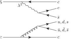
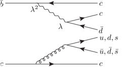

We will focus on the decay, avoiding the use of specific models. Heavy meson decays into two baryons are particularly suitable to extract the effective strong coupling which we expect to determine also the process we are interested in – both indeed contain six quarks confined in a two-hadron final state. In particular, one can consider[254, 255, 256]
| (204a) | |||
| (204b) | |||
These interactions can be described by mean of the following heavy meson chiral Lagrangian[172]:
| (205) |
where is a strong effective coupling and we take as for the -decay. represents both the and the , the dynamics of the two processes being the same. Fitting from the experimental data in Eqs. (204) one finds
| (206a) | ||||
| (206b) | ||||
which are compatible within the errors, thus suggesting that the internal dynamics might indeed be similar.
Extending this assuption to the decay we can take the effective coupling for this case, , to be the average of the previous two. The decay amplitudes can again be parametrized in terms of color structure, kinematics and the effective coupling. In Figure 49 we report the obtained results for both good and bad states and for a production associated with both a and a . One can notice that, if the is near threshold, than the branching ratio for an -wave production is just one order of magnitude smaller of the observed decays[257].
Summarizing, the theoretical study and the experimental search for possible exotic mesons with double flavor quantun numbers might be an interesting idea to further understand the nature of these particles. In particular, such particles might appear with double electric charge, in which case the only possible interpretation would be that of a compact tetraquark.
We also showed, that their widths and production branching fractions are large enought to be accessible at the present hadron facilities such as LCHb, ALICE, Tevatron and RHIC.
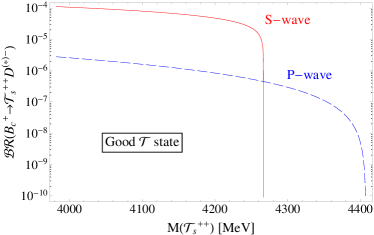
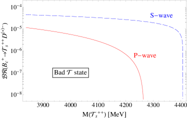
8.2 Compact tetraquarks and meson molecules in heavy ion collisions
Another possible tool to gain some insight about the nature of candidate tetraquarks is to study their behavior in the extreme conditions of relativistic heavy ion collisions at RHIC and LHC.
When two nuclei (Au+Au and Pb+Pb for RHIC and LHC respectively) collide at relativistic speed, the resulting system reaches extremely high temperatures. In particular, if those temperatures are higher than a critical value[258], MeV, quark and gluons are liberated from hadrons and a new state of matter is created, the so-called Quark-Gluon-Plasma (QGP). It is a QCD plasma of deconfined quarks and gluons which seems to behave as a nearly perfect fluid[259, 260]. After a certain amount of time this “fire-ball” expands and cools down to temperatures below and hence the partons confine again. In this phase the system looks like an expanding gas of interacting hadrons, the so-called Hadron Resonance Gas (HRG). When the temperature drops below the so-called freeze-out temperature, MeV[261], these hadrons simply fly apart without interacting anymore. In the following we will indicate with the subscripts , and quantities at the critical, hadronization and freeze-out temperatures respectively (see for example Table 8.2).
It has been proposed[262, 261, 263, 264] that the study of the produced number of exotic mesons, and in particular the time-honored , in heavy ion collisions might help to distinguish between the compact tetraquark picture and the molecular one. In particular, the two main techniques to estimate the yield of a particle in hot QGP are:
-
•
The statistical model[265]: it assumes that the matter produced in heavy ion collisions is in thermodynamical equilibrium and it is know to describe the relative yields of ordinary hadrons very well. In this model the number of hadrons of a given type, , produced is given by
(207) with being the degeneracy of and the volume (temperature) of the source when the statistical production of the hadron occurs. is the fugacity, with and the number of charm and anti-charm in the hadron, and the baryon and strangeness numbers of the hadron and and the corresponding chemical potentials.
This model does not contain any information about the actual internal structure of and, in the following, it will be used as a normalization factor.
-
•
The coalescence model[266]: it is based on the sudden approximation by calculating the overlap of the density matrix for the constituents of the hadron with the Wigner function for the produced particle. It is built to take into account the inner structure of , such as angular momentum, multiplicity of quarks, etc. This picture has successfully explained many different experimental data (e.g. enhancement of baryon production in the intermediate region[267], quark number scaling of the elliptic flow[268]). In this context, the number of hadrons produced is given by
(208) if one uses the non-relativistic approximation, neglect the transverse flow and considers only the unit rapidity. Moreover, one assumes an harmonic oscillator ansatz for the hadron internal structure. Here and are the degeneracy and number of the -th constituent and , with the oscillator frequency and the reduced mass given by . Lastly for a -wave and a -wave constituents respectively.
Note that from Eq. (208) follows that hadrons with more constituents are, in general, more suppressed and that S-wave coalescence if favored with respect to the P-wave one.
A large part of the information about the nature of the considered hadron is hence somehow embedded in the frequency of the harmonic oscillator. In the case of a compact multiquark state one can fit by requiring the coalescence model to reproduce the reference normal hadron yields in the statistical model. For the case of interest, the with light and charm quarks, one finds MeV by requiring the matching with the yield of [261]. The final result is a yield .
For the case of a meson molecule, instead, one can fix by using for a two-body -wave state, together with the equation that relates the binding energy of a loosely bound molecule with its scattering length, , and . For the case of the one gets MeV[261]. It is worth noting that and hence, according to Eq. (208), the smaller the binding energy of the molecule, the smaller and thus the larger is the . In this case it turns out to be .
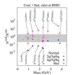
In Figure 50 the predicted yield for different hadrons in the coalescence model are shown[261]. As one immediately notices, the predictions for the compact tetraquark and for the molecule are completely different. In particular, a molecular structure for the implies a yield which is higher than ordinary hadrons, while a compact structure implies a lower yield. This difference is essentially due to the small binding energy of the molecular state and to the high number of constituents of the compact states. There is also another extremely striking feature, i.e. the predicted behaviors for the molecule and the compact tetraquark in relativistic heavy ion collisions are opposite to those predicted for collisions, as discussed in Sec. 6. Also note that both yields are close enough to the ordinary ones to be experimentally measured at RHIC and LHC.
The previous description of exotic mesons in heavy ion collision can be further improved[263]. So far we only studied the production during the QGP phase. However, the number of exotic mesons can also vary during the HRG phase, when disintegration/creation processes due to the interaction with other particles can occur. In particular, the most effective processes are – see Figure 51:
| (209a) | |||
| (209b) | |||
and the inverse ones for the creation of a . The vertices for such reaction can be obtained from an effective Lagrangian approach, with a combination of Heavy Quark Effective Theory (HQET) and chiral theory[263, 230]. In Figure 52 we report the cross sections for the processes in Eq. (209).
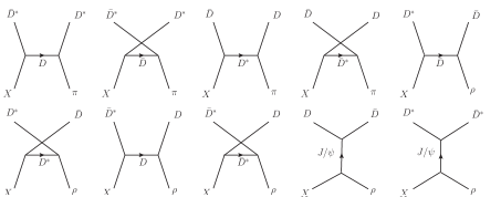

The computed cross sections can be used to estimate the change of the number of in the HRG as a function of the propert time, , by mean of kinetic theory[263]:
| (210) |
where the subscripts , and stand for a light meson and the two charmed mesons respectively. and are the density and abundancy of the particle at proper time calculated using the statistical model Eq. (207) with -dependent volume and temperature[263]:
| (211) |
These equations are obtained following the boost invariant Bjorken picture with an accelerated transverse expansion[269]. In particular, is the radius of the system at , and and are its expansion velocity and acceleration. In Table 8.2 we report the values used for the present analysis.
Values for the volume and temperature profiles in the schematic model of Eq. (211). Temp. (MeV) Time (fm/c) fm fm
The averages in Eq. (210) can be evaluated by mean of the kinetic theory:
| (212) |
with being the single particle density in momentum space. Lastly, the term is included to take into account the effect of the production of the through hadronization from the quark-gluon-plasma and is given by
| (213) |
is the number of produced by the quark-gluon-plasma as explained in Eqs. (207) and (208). Once all the ingredients are set one can compute the number of as a function of proper time, i.e. of the evolution of the hot expanding system. In Figure 53 we report the results for central Au-Au collisions at GeV.

The number of in the assumption of a molecular nature can be computed by solving the evolution equation (210) backward in time, starting from the yield found before using the coalescence model, . The result is again shown in Figure 53.
As one can see, the inclusion of this further possible mechanism of creation/destruction of the , i.e. the interaction of this meson in the hadron resonance gas, leads to a yield for an eventual molecular state which is a factor of larger than that for a compact four-quark structure.
It should be noted that the previous discussion completely neglects transverse flow effects. However, this phenomena turned out to be the key ingredient to explain some puzzling experimental results like, for example, the observation made at RHIC that medium-induced suppression for values of the transverse momentum GeV is not as effective on protons as it is for pions[270, 271]. Particularly surprising was the fact that the ratio of protons over charged pions for transverse momenta above GeV reaches or even exceeds unity. The explanation to this phenomenon was the following. The expectation from the use of coalescence model is that it is less likely to bind states made by a larger number of components simply because the convolution of their wave functions is smaller. In other words, it is hard to find the components at small value of the relative momentum and at small relative positions. However, if one takes into account flow effects it turns out that, exactly because of collectivity, if the previously mentioned components are found close in momentum space, they are also likely to be close in coordinate space, thus increasing the yield of states with higher number of constituents. As we said, this effect turned out to be relevant at explaining the observed ratio for GeV.
In our case, this phenomenon might be quite important at increasing the number of tetraquarks produced with respect to the number of molecules [272, 273]. Therefore, in our view, the conclusions drawn in Fig. 50 are merely partial.
In conclusion, we showed how the study of the yield of – and possibly of other exotic mesons – in heavy ion collisions might have an impact on the determination of its nature. In particular, it turns out that, according to the coalescence model[266], the number of produced should be much larger if it is a loosely bound molecule than if it is compact tetraquark, in strking contrast to what expected for collisions. Moreover, the predicted yields[261, 263] are large enough to be measurable by the current experimental facilities, RHIC and LHC. Future studies should try to include collective flow effects as well.
Sec. 9 Comparisons
In this section we would like to recollect the various predictions made by different models in a way as complete as possible to the best of our knowledge. Such predictions will include both production and decay of the exotic mesons considered in this review. Moreover, we would like to stress how, in our opinion, because of the unavoidable amount of assumptions/approximations made by every model, the following results should mainly be considered as order of magnitude estimates, even when statistical uncertainties are quoted. In Tables 9 and 9 we report the predictions for many quantities and different models, together with the references where they can be found.
Recollection of predictions for different models and different channels involving both the production and decay of exotic states. We remind to the reader that NREFT stands for Non-Relativistic Effective Field Theory and that NREFT-II stands for Non-Relativistic Effective Field Theory Type II – see Sec. 5.1.2. Quantity Model Ref. Prediction Mol. (NREFT) (Sec. 5.1.2) [170] keV Mol. (NREFT) (Sec. 5.1.2) [170] keV Mol. (NREFT) (Sec. 5.1.2) [170] keV Mol. (NREFT) (Sec. 5.1.2) [170] keV Mol. (NREFT) (Sec. 5.1.2) [167] Mol. (NREFT) (Sec. 5.1.2) [167] Mol. (NREFT) (Sec. 5.1.2) [167] Mol. (NREFT) (Sec. 5.1.2) [167] Mol. (NREFT) (Sec. 5.1.2) [167] Mol. (NREFT) (Sec. 5.1.2) [167] Mol. (NREFT) (Sec. 5.1.2) [167] Mol. (NREFT) (Sec. 5.1.2) [167] Mol. (NREFT) (Sec. 5.1.2) [167] Mol. (NREFT) (Sec. 5.1.2) [167] Mol. (NREFT) (Sec. 5.1.2) [167] Mol. (NREFT) (Sec. 5.1.2) [167] Mol. (NREFT) (Sec. 5.1.2) [167] Mol. (NREFT) (Sec. 5.1.2) [167] Mol. (NREFT) (Sec. 5.1.2) [167] Mol. (NREFT) (Sec. 5.1.2) [167] Mol. (NREFT) (Sec. 5.1.2) [167] Mol. (Low-energy univ.) (Sec. 5.1.1) [159] keV Mol. (Low-energy univ.) (Sec. 5.1.1) [159] suppressed as Mol. (Low-energy univ.) (Sec. 5.1.1) [159] suppressed as Mol. (Low-energy univ.) (Sec. 5.1.1) [159] suppressed as Mol. (Low-energy univ.) (Sec. 5.1.1) [159] suppressed as Mol. (NREFT-II) (Sec. 5.1.2) [165] keV Mol. in Heavy-Ion coll. (Sec. 8.2) [263] Tetraq. in Heavy-Ion coll. (Sec. 8.2) [263]
(Continued). We remind to the reader that QCDSR stands for QCD Sum Rules. Moreover, with “no dynamics” and “dynamics incl.” we refer to the exclusion or inclusion of the recent dynamical model developed by Brodsky et al.[242] to compute the tetraquark effective couplings to quarkonia. Quantity Model Ref. Prediction Mol. (NREFT) (Sec. 5.1.2) [171] Mol. (NREFT) (Sec. 5.1.2) [171] Mol. (NREFT) (Sec. 5.1.2) [171] Mol. (NREFT) (Sec. 5.1.2) [171] Tetraq. (Type-I no dynam.) (Sec. 7.7) [171] Tetraq. (Type-II no dynam.) (Sec. 7.7) [171] Tetraq. (Type-I dynam. incl.) (Sec. 7.7) [171] Tetraq. (Type-II dynam. incl.) (Sec. 7.7) [171] Tetraq. (Type-I no dynam.) (Sec. 7.7) [171] Tetraq. (Type-II no dynam.) (Sec. 7.7) [171] Tetraq. (Type-I dynam. incl.) (Sec. 7.7) [171] Tetraq. (Type-II dynam. incl.) (Sec. 7.7) [171] Tetraq. (no dynam.) (Sec. 8.1) [6] (near thresh.) Tetraq. (no dynam.) (Sec. 8.1) [6] (near thresh.) Tetraq. (no dynam.) (Sec. 8.1) [6] (near thresh.) Tetraq. (no dynam.) (Sec. 8.1) [6] (near thresh.) Hadro-charm. (Sec. 5.2) [174] few MeV Hadro-charm. (Sec. 5.2) [174] few MeV Hadro-charm. (Sec. 5.2) [174] few MeV Hadro-charm. (Sec. 5.2) [174] few MeV Pure mol. or tetraq. (QCDSR) (Sec. 7.7.1) [245] Pure tetraq. (QCDSR) (Sec. 7.7.1) [245] MeV Mix. of mol. and (QCDSR) (Sec. 7.7.1) [245] MeV Mix. of mol. and (QCDSR) (Sec. 7.7.1) [274] Pure tetraq. (QCDSR) (Sec. 7.7.1) [275] MeV Pure tetraq. (QCDSR) (Sec. 7.7.1) [275] MeV Pure tetraq. (QCDSR) (Sec. 7.7.1) [275] MeV Pure tetraq. (QCDSR) (Sec. 7.7.1) [275] MeV Pure tetraq. (QCDSR) (Sec. 7.7.1) [276] MeV Pure tetraq. (QCDSR) (Sec. 7.7.1) [276] MeV
Sec. 10 Conclusions
The field of phenomenology has impressively been growing on the experimental side. On the other hand it seems that the theoretical models to explain the rich amount of information nowadays available on these states are lagging behind. One of the reasons for this is maybe due to the narrow number of active researcher in the field, especially those culturally close to high-energy physics. particles are observed in high-energy reactions, at high transverse momenta, as we know from the recent findings by LHCb, CMS and, even more recently, by ATLAS. For these reasons they are unlikely to be the manifestations of some nuclear force type dynamics. We are also very skeptical about interpreting most of them in terms of kinematical effects, as claimed by some authors.
In this review we have tried to highlight the reasons for the most fundamental quark picture, suggesting these states to be new kinds of hadrons with respect to standard mesons and baryons, namely new bodyplans of quarks arranged into tetraquarks. The possibility of having long-lived tetraquarks is not excluded by the large number of colors limit of QCD and, in addition, some of the observed charged resonances appear as striking evidence that compact tetraquarks have already been observed. The simplified diquark-antidiquark model reviewed in this paper is not the definitive explanation of the resonances, but we believe it must be at the core of the picture. One still has to explain what prevents some of the states predicted by that model to be formed/observed in experiment. We started by looking for the origin of such selection rules in the accidental matchings of diquark-antidiquark levels with open charm (beauty) meson thresholds. We do not think that there is anything profound in these matchings, given the huge number of thresholds which can be formed with the known pairs of charmed or beauty mesons. However tetraquark discrete levels might correspond to narrow hadron resonances whenever anyone of these matchings happens to be realized. This is probably the passage to be done to fill the gap between the tetraquark interpretation and the actual phenomenology of these resonances.
In this respects it may be true that we are looking at different aspects of the same problem using different descriptions, as considered by someone. It may also be true that the definitive answer could be in the non-perturbative intricacies of strong interactions which might eventually be captured only using lattice QCD methods. Yet, in the meanwhile, we think that we made some interesting and solid progress, and especially we believe that there is indeed a problem in resonance physics: whatever side you are looking at it, it is not a “mirage” made of effects, cusps, particular cases. It looks like there is a pattern behind.
Acknowledgements
We wish to thank R. Faccini, G. Filaci, B. Grinstein, F. Renga, M. Papinutto, C. Sabelli, N. Tantalo, M. Testa and especially L. Maiani and V. Riquer-Ramirez for many stimulating discussions and a very fruitful collaboration.
References
- [1] G. ‘t Hooft, Nucl.Phys. B75, 461 (1974).
- [2] E. Witten, Nucl.Phys. B160, 57 (1979).
- [3] S. Coleman, Aspects of Symmetry (Cambridge University Press, Cambridge, England, 1985).
- [4] S. Weinberg, Phys.Rev.Lett. 110, 261601 (2013), arXiv:1303.0342 [hep-ph].
- [5] M. Knecht and S. Peris, Phys.Rev. D88, 036016 (2013), arXiv:1307.1273 [hep-ph].
- [6] A. Esposito, M. Papinutto, A. Pilloni, A. Polosa and N. Tantalo, Phys.Rev. D88, 054029 (2013), arXiv:1307.2873 [hep-ph].
- [7] L. Maiani, F. Piccinini, A. Polosa and V. Riquer, Phys.Rev.Lett. 93, 212002 (2004), arXiv:hep-ph/0407017 [hep-ph].
- [8] R. F. Lebed, Phys.Rev. D88, 057901 (2013), arXiv:1308.2657 [hep-ph].
- [9] G. Veneziano, Nucl.Phys. B117, 519 (1976).
- [10] E. Corrigan and P. Ramond, Phys.Lett. B87, 73 (1979).
- [11] T. D. Cohen and R. F. Lebed, Phys.Rev. D89, 054018 (2014), arXiv:1401.1815 [hep-ph].
- [12] S. Prelovsek and L. Leskovec, Phys.Rev.Lett. 111, 192001 (2013), arXiv:1307.5172 [hep-lat].
- [13] S. Prelovsek and L. Leskovec, Phys.Lett. B727, 172 (2013), arXiv:1308.2097 [hep-lat].
- [14] S. Prelovsek, C. Lang, L. Leskovec and D. Mohler (2014), arXiv:1405.7623 [hep-lat].
- [15] M. Wagner, A. Abdel-Rehim, C. Alexandrou, M. Dalla Brida, M. Gravina et al., J.Phys.Conf.Ser. 503, 012031 (2014), arXiv:1310.6905 [hep-lat].
- [16] C. Alexandrou, J. O. Daldrop, M. Dalla Brida, M. Gravina, L. Scorzato et al., JHEP 1304, 137 (2013), arXiv:1212.1418.
- [17] T. D. Cohen and R. F. Lebed, Phys.Rev. D90, 016001 (2014), arXiv:1403.8090 [hep-ph].
- [18] S. F. Radford and W. W. Repko, Phys.Rev. D75, 074031 (2007), arXiv:hep-ph/0701117 [hep-ph].
- [19] C.-N. Yang, Phys.Rev. 77, 242 (1950).
- [20] N. Drenska, R. Faccini, F. Piccinini, A. Polosa, F. Renga and C. Sabelli, Riv.Nuovo Cim. 033, 633 (2010), arXiv:1006.2741 [hep-ph].
- [21] R. Faccini, A. Pilloni and A. D. Polosa, Mod.Phys.Lett. A27, 1230025 (2012), arXiv:1209.0107 [hep-ph].
- [22] BABAR Collaboration, Belle Collaboration (A. Bevan et al.) (2014), arXiv:1406.6311 [hep-ex].
- [23] Belle Collaboration (V. Bhardwaj et al.), Phys.Rev.Lett. 111, 032001 (2013), arXiv:1304.3975 [hep-ex].
- [24] Belle Collaboration (S.-K. Choi et al.), Phys.Rev.Lett. 91, 262001 (2003), arXiv:hep-ex/0309032.
- [25] S.-K. Choi, S. L. Olsen, K. Trabelsi, I. Adachi, H. Aihara et al., Phys.Rev. D84, 052004 (2011), arXiv:1107.0163 [hep-ex].
- [26] BABAR Collaboration (B. Aubert et al.), Phys.Rev. D77, 111101 (2008), arXiv:0803.2838 [hep-ex].
- [27] CDF Collaboration (A. Abulencia et al.), Phys.Rev.Lett. 98, 132002 (2007), arXiv:hep-ex/0612053 [hep-ex].
- [28] CDF Collaboration (T. Aaltonen et al.), Phys.Rev.Lett. 103, 152001 (2009), arXiv:0906.5218 [hep-ex].
- [29] D Collaboration (V. Abazov et al.), Phys.Rev.Lett. 93, 162002 (2004), arXiv:hep-ex/0405004 [hep-ex].
- [30] LHCb Collaboration (R. Aaij et al.), Eur.Phys.J. C72, 1972 (2012), arXiv:1112.5310 [hep-ex].
- [31] LHCb Collaboration (R. Aaij et al.), Phys.Rev.Lett. 110, 222001 (2013), arXiv:1302.6269 [hep-ex].
- [32] Belle Collaboration (K. Abe et al.) (2005), arXiv:hep-ex/0505037 [hep-ex].
- [33] BABAR Collaboration (P. del Amo Sanchez et al.), Phys.Rev. D82, 011101 (2010), arXiv:1005.5190 [hep-ex].
- [34] Belle Collaboration (V. Bhardwaj et al.), Phys.Rev.Lett. 107, 9 (2011), arXiv:1105.0177 [hep-ex].
- [35] BABAR Collaboration (B. Aubert et al.), Phys.Rev.Lett. 102, 132001 (2009), arXiv:0809.0042 [hep-ex].
- [36] LHCb Collaboration (R. Aaij et al.), Nucl.Phys. B886, 665 (2014), arXiv:1404.0275 [hep-ex].
- [37] Belle Collaboration (T. Aushev et al.), Phys.Rev. D81, 031103 (2010), arXiv:0810.0358 [hep-ex].
- [38] BABAR Collaboration (B. Aubert et al.), Phys.Rev. D77, 011102 (2008), arXiv:0708.1565 [hep-ex].
- [39] BESIII Collaboration (M. Ablikim et al.), Phys.Rev.Lett. 112, 022001 (2014), arXiv:1310.1163 [hep-ex].
- [40] BESIII Collaboration (M. Ablikim et al.), Phys.Rev.Lett. 110, 252001 (2013), arXiv:1303.5949 [hep-ex].
- [41] Belle Collaboration (Z. Liu et al.), Phys.Rev.Lett. 110, 252002 (2013), arXiv:1304.0121 [hep-ex].
- [42] T. Xiao, S. Dobbs, A. Tomaradze and K. K. Seth, Phys.Lett. B727, 366 (2013), arXiv:1304.3036 [hep-ex].
- [43] BESIII Collaboration (M. Ablikim et al.), Phys.Rev.Lett. 111, 242001 (2013), arXiv:1309.1896 [hep-ex].
- [44] BESIII Collaboration (M. Ablikim et al.), Phys.Rev.Lett. 112, 132001 (2014), arXiv:1308.2760 [hep-ex].
- [45] Belle Collaboration (K. Abe et al.), Phys.Rev.Lett. 94, 182002 (2005), arXiv:hep-ex/0408126.
- [46] BABAR Collaboration (B. Aubert et al.), Phys.Rev.Lett. 101, 082001 (2008), arXiv:0711.2047 [hep-ex].
- [47] Belle Collaboration (S. Uehara et al.), Phys.Rev.Lett. 104, 092001 (2010), arXiv:0912.4451 [hep-ex].
- [48] BABAR Collaboration (J. P. Lees et al.), Phys.Rev. D86, 072002 (2012), arXiv:1207.2651 [hep-ex].
- [49] Belle Collaboration (S. Uehara et al.), Phys.Rev.Lett. 96, 082003 (2006), arXiv:hep-ex/0512035.
- [50] BABAR Collaboration (B. Aubert et al.), Phys.Rev. D81, 092003 (2010), arXiv:1002.0281 [hep-ex].
- [51] Belle Collaboration (K. Abe et al.), Phys.Rev.Lett. 98, 082001 (2007), arXiv:hep-ex/0507019.
- [52] Belle Collaboration (P. Pakhlov et al.), Phys.Rev.Lett. 100, 202001 (2008), arXiv:0708.3812 [hep-ex].
- [53] Belle Collaboration (C. Z. Yuan et al.), Phys.Rev.Lett. 99, 182004 (2007), arXiv:0707.2541 [hep-ex].
- [54] Belle Collaboration (R. Mizuk et al.), Phys.Rev. D78, 072004 (2008), arXiv:0806.4098 [hep-ex].
- [55] BABAR Collaboration (J. P. Lees et al.), Phys.Rev. D85, 052003 (2012), arXiv:1111.5919 [hep-ex].
- [56] CDF Collaboration (T. Aaltonen et al.), Phys.Rev.Lett. 102, 242002 (2009), arXiv:0903.2229 [hep-ex].
- [57] CDF Collaboration (T. Aaltonen et al.) (2011), arXiv:1101.6058 [hep-ex].
- [58] Belle Collaboration (C. P. Shen et al.), Phys.Rev.Lett. 104, 112004 (2010), arXiv:0912.2383 [hep-ex].
- [59] LHCb Collaboration (R. Aaij et al.), Phys.Rev. D85, 091103 (2012), arXiv:1202.5087 [hep-ex].
- [60] CMS Collaboration (S. Chatrchyan et al.), Phys.Lett. B734, 261 (2014), arXiv:1309.6920 [hep-ex].
- [61] D Collaboration (V. M. Abazov et al.), Phys.Rev. D89, 012004 (2014), arXiv:1309.6580 [hep-ex].
- [62] Belle Collaboration (K. Chilikin et al.), Phys.Rev. D90, 112009 (2014), arXiv:1408.6457 [hep-ex].
- [63] C.-Z. Yuan, Chin.Phys. C38, 043001 (2014), arXiv:1312.6399 [hep-ex].
- [64] C.-Z. Yuan, Int.J.Mod.Phys. A29, 1430046 (2014), arXiv:1404.7768 [hep-ex].
- [65] BES III Collaboration (M. Ablikim et al.) (2014), arXiv:1410.6538 [hep-ex].
- [66] BABAR Collaboration (B. Aubert et al.), Phys.Rev.Lett. 95, 142001 (2005), arXiv:hep-ex/0506081.
- [67] BABAR Collaboration (J. P. Lees et al.), Phys.Rev. D86, 051102 (2012), arXiv:1204.2158 [hep-ex].
- [68] CLEO Collaboration (T. E. Coan et al.), Phys.Rev.Lett. 96, 162003 (2006), arXiv:hep-ex/0602034 [hep-ex].
- [69] CLEO Collaboration (Q. He et al.), Phys.Rev. D74, 091104 (2006), arXiv:hep-ex/0611021 [hep-ex].
- [70] BESIII Collaboration (M. Ablikim et al.), Phys.Rev.Lett. 112, 092001 (2014), arXiv:1310.4101 [hep-ex].
- [71] Belle Collaboration (X. L. Wang et al.), Phys.Rev.Lett. 99, 142002 (2007), arXiv:0707.3699 [hep-ex].
- [72] BABAR Collaboration (J. Lees et al.), Phys.Rev. D89, 111103 (2014), arXiv:1211.6271 [hep-ex].
- [73] Belle Collaboration (R. Mizuk et al.), Phys.Rev. D80, 031104 (2009), arXiv:0905.2869 [hep-ex].
- [74] Belle Collaboration (K. Chilikin et al.), Phys.Rev. D88, 074026 (2013), arXiv:1306.4894 [hep-ex].
- [75] BABAR Collaboration (B. Aubert et al.), Phys.Rev. D79, 112001 (2009), arXiv:0811.0564 [hep-ex].
- [76] LHCb Collaboration (R. Aaij et al.), Phys.Rev.Lett. 112, 222002 (2014), arXiv:1404.1903 [hep-ex].
- [77] Belle Collaboration (G. Pakhlova et al.), Phys.Rev.Lett. 101, 172001 (2008), arXiv:0807.4458 [hep-ex].
- [78] Belle Collaboration (A. Bondar et al.), Phys.Rev.Lett. 108, 122001 (2012), arXiv:1110.2251 [hep-ex].
- [79] Belle Collaboration (P. Krokovny et al.), Phys.Rev. D88, 052016 (2013), arXiv:1308.2646 [hep-ex].
- [80] Belle Collaboration (I. Adachi et al.) (2012), arXiv:1209.6450 [hep-ex].
- [81] Belle Collaboration (S.-K. Choi et al.), Phys.Rev.Lett. 100, 142001 (2008), arXiv:0708.1790 [hep-ex].
- [82] D. Bugg, J.Phys. G35, 075005 (2008), arXiv:0802.0934 [hep-ph].
- [83] C.-Z. Yuan, The states at besiii. http://indico.cern.ch/event/278195/session/0/contribution/4/material/slides/0.pdf.
- [84] Particle Data Group Collaboration (K. Olive et al.), Chin.Phys. C38, 090001 (2014).
- [85] BESIII Collaboration (M. Ablikim et al.), Phys.Rev.Lett. 113, 212002 (2014), arXiv:1409.6577 [hep-ex].
- [86] COMPASS Collaboration (C. Adolph et al.) (2014), arXiv:1407.6186 [hep-ex].
- [87] Belle Collaboration (X. Wang, C. Yuan, C. Shen, P. Wang, A. Abdesselam et al.) (2014), arXiv:1410.7641 [hep-ex].
- [88] Belle Collaboration (K.-F. Chen et al.), Phys.Rev.Lett. 100, 112001 (2008), arXiv:0710.2577 [hep-ex].
- [89] Belle Collaboration (I. Adachi et al.), Phys.Rev.Lett. 108, 032001 (2012), arXiv:1103.3419 [hep-ex].
- [90] Belle Collaboration (A. Garmash et al.) (2014), arXiv:1403.0992 [hep-ex].
- [91] BABAR Collaboration (B. Aubert et al.), Phys.Rev. D71, 071103 (2005), arXiv:hep-ex/0406022.
- [92] CDF Collaboration (D. Acosta et al.), Phys.Rev.Lett. 93, 072001 (2004), arXiv:hep-ex/0312021 [hep-ex].
- [93] CMS Collaboration (S. Chatrchyan et al.), JHEP 1304, 154 (2013), arXiv:1302.3968 [hep-ex].
- [94] CDF Collaboration (A. Abulencia et al.), Phys.Rev.Lett. 96, 102002 (2006), arXiv:hep-ex/0512074 [hep-ex].
- [95] BABAR Collaboration (B. Aubert et al.), Phys.Rev. D74, 071101 (2006), arXiv:hep-ex/0607050.
- [96] Belle Collaboration (K. Abe et al.) (2005), arXiv:hep-ex/0505038 [hep-ex].
- [97] T. J. Burns, F. Piccinini, A. D. Polosa and C. Sabelli, Phys.Rev. D82, 074003 (2010), arXiv:1008.0018 [hep-ph].
- [98] C. Hanhart, Y. S. Kalashnikova, A. E. Kudryavtsev and A. V. Nefediev, Phys.Rev. D85, 011501 (2012), arXiv:1111.6241 [hep-ph].
- [99] R. Faccini, F. Piccinini, A. Pilloni and A. Polosa, Phys.Rev. D86, 054012 (2012), arXiv:1204.1223 [hep-ph].
- [100] E. Braaten and D. Kang, Phys.Rev. D88, 014028 (2013), arXiv:1305.5564 [hep-ph].
- [101] CLEO Collaboration (S. Dobbs et al.), Phys.Rev.Lett. 94, 032004 (2005), arXiv:hep-ex/0410038 [hep-ex].
- [102] Belle Collaboration (G. Gokhroo et al.), Phys.Rev.Lett. 97, 162002 (2006), arXiv:hep-ex/0606055.
- [103] P. Artoisenet, E. Braaten and D. Kang, Phys.Rev. D82, 014013 (2010), arXiv:1005.2167 [hep-ph].
- [104] C. Hanhart, Y. S. Kalashnikova and A. V. Nefediev, Phys.Rev. D81, 094028 (2010), arXiv:1002.4097 [hep-ph].
- [105] C. Hanhart, Y. S. Kalashnikova and A. V. Nefediev, Eur.Phys.J. A47, 101 (2011), arXiv:1106.1185 [hep-ph].
- [106] Belle Collaboration (I. Adachi et al.) (2008), arXiv:0809.1224 [hep-ex].
- [107] BABAR Collaboration (B. Aubert et al.), Phys.Rev.Lett. 96, 052002 (2006), arXiv:hep-ex/0510070.
- [108] BABAR Collaboration (B. Aubert et al.), Phys.Rev. D73, 011101 (2006), arXiv:hep-ex/0507090.
- [109] BABAR Collaboration (B. Aubert et al.), Phys.Rev. D71, 031501 (2005), arXiv:hep-ex/0412051.
- [110] LHCb Collaboration (R. Aaij et al.), Eur.Phys.J. C73, 2462 (2013), arXiv:1303.7133 [hep-ex].
- [111] Belle Collaboration (K. Abe et al.), Phys.Lett. B662, 323 (2008), arXiv:hep-ex/0608037.
- [112] BABAR Collaboration (B. Aubert et al.), Phys.Rev.Lett. 93, 041801 (2004), arXiv:hep-ex/0402025.
- [113] CDF II Collaboration, The “Lifetime” Distribution of Mesons Produced in Collisions at CDF http://www-cdf.fnal.gov/physics/new/bottom/051020.blessed-X3872/XLife/xlonglivedWWW.ps, CDF note 7159.
- [114] C. Bignamini, B. Grinstein, F. Piccinini, A. Polosa and C. Sabelli, Phys.Rev.Lett. 103, 162001 (2009), arXiv:0906.0882 [hep-ph].
- [115] BABAR Collaboration (B. Aubert et al.), Phys.Rev.Lett. 98, 212001 (2007), arXiv:hep-ex/0610057.
- [116] G. Cotugno, R. Faccini, A. Polosa and C. Sabelli, Phys.Rev.Lett. 104, 132005 (2010), arXiv:0911.2178 [hep-ph].
- [117] BABAR Collaboration (B. Aubert et al.), Phys.Rev.Lett. 99, 071801 (2007), arXiv:0705.1190 [hep-ex].
- [118] BABAR Collaboration (P. del Amo Sanchez et al.), Phys.Rev. D82, 052004 (2010), arXiv:1008.0338 [hep-ex].
- [119] Belle Collaboration (G. Pakhlova et al.), Phys.Rev. D80, 091101 (2009), arXiv:0908.0231 [hep-ex].
- [120] Belle Collaboration (C. Yuan et al.), Phys.Rev. D77, 011105 (2008), arXiv:0709.2565 [hep-ex].
- [121] Belle Collaboration (X. Wang, Y. Han, C. Yuan, C. Shen and P. Wang), Phys.Rev. D87, 051101 (2013), arXiv:1210.7550 [hep-ex].
- [122] BABAR Collaboration (B. Aubert et al.), Phys.Rev. D76, 012008 (2007), arXiv:0704.0630 [hep-ex].
- [123] BABAR Collaboration (B. Aubert et al.), Phys.Rev. D77, 092002 (2008), arXiv:0710.4451 [hep-ex].
- [124] CLEO Collaboration (T. Pedlar et al.), Phys.Rev.Lett. 107, 041803 (2011), arXiv:1104.2025 [hep-ex].
- [125] BABAR Collaboration (B. Aubert et al.), Phys.Rev. D73, 012005 (2006), arXiv:hep-ex/0512023 [hep-ex].
- [126] Belle Collaboration (J. Brodzicka et al.), Phys.Rev.Lett. 100, 092001 (2008), arXiv:0707.3491 [hep-ex].
- [127] T. Barnes, S. Godfrey and E. Swanson, Phys.Rev. D72, 054026 (2005), arXiv:hep-ph/0505002 [hep-ph].
- [128] F.-K. Guo and U.-G. Meissner, Phys.Rev. D86, 091501 (2012), arXiv:1208.1134 [hep-ph].
- [129] S. L. Olsen (2014), arXiv:1410.6534 [hep-ex].
- [130] T. Branz, T. Gutsche and V. E. Lyubovitskij, Phys.Rev. D80, 054019 (2009), arXiv:0903.5424 [hep-ph].
- [131] BABAR Collaboration (J. Lees et al.) (2014), arXiv:1407.7244 [hep-ex].
- [132] BES III Collaboration (M. Ablikim et al.) (2014), arXiv:1412.1867 [hep-ex].
- [133] Hadron Spectrum Collaboration (L. Liu et al.), JHEP 1207, 126 (2012), arXiv:1204.5425 [hep-ph].
- [134] M. Luscher and U. Wolff, Nucl.Phys. B339, 222 (1990).
- [135] S. Prelovsek, PoS LATTICE2014, 015 (2014), arXiv:1411.0405 [hep-lat].
- [136] L. Maiani and M. Testa, Phys.Lett. B245, 585 (1990).
- [137] M. Lüscher, Nucl.Phys. B354, 531 (1991).
- [138] M. Lüscher, Nucl.Phys. B364, 237 (1991).
- [139] S. Sasaki and T. Yamazaki, Phys.Rev. D74, 114507 (2006), arXiv:hep-lat/0610081 [hep-lat].
- [140] Y. Chen, M. Gong, Y.-H. Lei, N. Li, J. Liang et al., Phys.Rev. D89, 094506 (2014), arXiv:1403.1318 [hep-lat].
- [141] N. A. Tornqvist, Phys.Rev.Lett. 67, 556 (1991).
- [142] T. E. O. Ericson and G. Karl, Phys.Lett. B309, 426 (1993).
- [143] A. De Rujula, H. Georgi and S. Glashow, Phys.Rev.Lett. 38, 317 (1977).
- [144] M. Voloshin and L. Okun, JETP Lett. 23, 333 (1976).
- [145] N. A. Tornqvist, Z.Phys. C61, 525 (1994), arXiv:hep-ph/9310247 [hep-ph].
- [146] A. V. Manohar and M. B. Wise, Nucl.Phys. B399, 17 (1993), arXiv:hep-ph/9212236 [hep-ph].
- [147] E. S. Swanson, Annals Phys. 220, 73 (1992).
- [148] Y. Kalashnikova and A. Nefediev, Pisma Zh.Eksp.Teor.Fiz. 97, 76 (2013), arXiv:1212.2004 [hep-ph].
- [149] N. A. Tornqvist, Phys.Lett. B590, 209 (2004), arXiv:hep-ph/0402237 [hep-ph], This report supersedes the unpublished reminder hep-ph/0308277.
- [150] T. Barnes and E. Swanson, Phys.Rev. D46, 131 (1992).
- [151] E. S. Swanson, Phys.Rept. 429, 243 (2006), arXiv:hep-ph/0601110 [hep-ph].
- [152] E. S. Swanson, Phys.Lett. B588, 189 (2004), arXiv:hep-ph/0311229 [hep-ph].
- [153] A. Bondar, A. Garmash, A. Milstein, R. Mizuk and M. Voloshin, Phys.Rev. D84, 054010 (2011), arXiv:1105.4473 [hep-ph].
- [154] F.-K. Guo, C. Hanhart and U.-G. Meissner, Phys.Rev.Lett. 102, 242004 (2009), arXiv:0904.3338 [hep-ph].
- [155] F.-K. Guo, C. Hidalgo-Duque, J. Nieves and M. P. Valderrama, Phys.Rev. D88, 054007 (2013), arXiv:1303.6608 [hep-ph].
- [156] A. Tomaradze, S. Dobbs, T. Xiao, K. K. Seth and G. Bonvicini (2012), arXiv:1212.4191 [hep-ex].
- [157] M. Voloshin, Phys.Lett. B579, 316 (2004), arXiv:hep-ph/0309307 [hep-ph].
- [158] A. Esposito, F. Piccinini, A. Pilloni and A. Polosa, J.Mod.Phys. 4, 1569 (2013), arXiv:1305.0527 [hep-ph].
- [159] E. Braaten and M. Kusunoki, Phys.Rev. D69, 074005 (2004), arXiv:hep-ph/0311147 [hep-ph].
- [160] A. J. Leggett, Quantum liquids: Bose condensation and Cooper pairing in condensed-matter systems (Oxford University Press, 2006).
- [161] C. Hanhart, Y. Kalashnikova, A. E. Kudryavtsev and A. Nefediev, Phys.Rev. D76, 034007 (2007), arXiv:0704.0605 [hep-ph].
- [162] E. Braaten and M. Lu, Phys.Rev. D76, 094028 (2007), arXiv:0709.2697 [hep-ph].
- [163] E. Braaten and J. Stapleton, Phys.Rev. D81, 014019 (2010), arXiv:0907.3167 [hep-ph].
- [164] E. Braaten and M. Lu, Phys.Rev. D79, 051503 (2009), arXiv:0712.3885 [hep-ph].
- [165] S. Fleming, M. Kusunoki, T. Mehen and U. van Kolck, Phys.Rev. D76, 034006 (2007), arXiv:hep-ph/0703168 [hep-ph].
- [166] M. Cleven, F.-K. Guo, C. Hanhart and U.-G. Meissner, Eur.Phys.J. A47, 120 (2011), arXiv:1107.0254 [hep-ph].
- [167] M. Cleven, Q. Wang, F.-K. Guo, C. Hanhart, U.-G. Meissner et al., Phys.Rev. D87, 074006 (2013), arXiv:1301.6461 [hep-ph].
- [168] M. Cleven (2014), arXiv:1405.4195 [hep-ph].
- [169] Q. Wang, C. Hanhart and Q. Zhao, Phys.Rev.Lett. 111, 132003 (2013), arXiv:1303.6355 [hep-ph].
- [170] F.-K. Guo, C. Hanhart, U.-G. Mei ner, Q. Wang and Q. Zhao, Phys.Lett. B725, 127 (2013), arXiv:1306.3096 [hep-ph].
- [171] A. Esposito, A. Guerrieri and A. Pilloni (2014), arXiv:1409.3551 [hep-ph].
- [172] R. Casalbuoni, A. Deandrea, N. Di Bartolomeo, R. Gatto, F. Feruglio et al., Phys.Rept. 281, 145 (1997), arXiv:hep-ph/9605342 [hep-ph].
- [173] A. Manohar and M. Wise, Heavy Quark Physics (Cambridge University Press, 2007).
- [174] S. Dubynskiy and M. Voloshin, Phys.Lett. B666, 344 (2008), arXiv:0803.2224 [hep-ph].
- [175] S. Dubynskiy, A. Gorsky and M. Voloshin, Phys.Lett. B671, 82 (2009), arXiv:0804.2244 [hep-th].
- [176] S. J. Brodsky, I. Schmidt and G. de Teramond, Phys.Rev.Lett. 64, 1011 (1990).
- [177] M. Voloshin, Mod.Phys.Lett. A19, 665 (2004), arXiv:hep-ph/0402011 [hep-ph].
- [178] X. Li and M. Voloshin, Mod.Phys.Lett. A29, 1450060 (2014), arXiv:1309.1681 [hep-ph].
- [179] R. Jaffe and K. Johnson, Phys.Lett. B60, 201 (1976).
- [180] T. Barnes and F. Close, Phys.Lett. B116, 365 (1982).
- [181] T. Barnes, F. Close, F. de Viron and J. Weyers, Nucl.Phys. B224, 241 (1983).
- [182] P. Hasenfratz, R. Horgan, J. Kuti and J. Richard, Phys.Lett. B95, 299 (1980).
- [183] Y. Kalashnikova and D. Kuzmenko, Phys.Atom.Nucl. 66, 955 (2003), arXiv:hep-ph/0203128 [hep-ph].
- [184] D. Horn and J. Mandula, Phys.Rev. D17, 898 (1978).
- [185] M. Tanimoto, Phys.Lett. B116, 198 (1982).
- [186] M. Tanimoto, Phys.Rev. D27, 2648 (1983).
- [187] F. Iddir, A. Le Yaouanc, L. Oliver, O. Pene, J. Raynal et al., Phys.Lett. B205, 564 (1988).
- [188] S. Ishida, H. Sawazaki, M. Oda and K. Yamada, Phys.Rev. D47, 179 (1993).
- [189] S. Ishida, M. Oda, H. Sawazaki and K. Yamada, Prog.Theor.Phys. 82, 119 (1989).
- [190] T. Barnes, F. Close and E. Swanson, Phys.Rev. D52, 5242 (1995), arXiv:hep-ph/9501405 [hep-ph].
- [191] S. Perantonis and C. Michael, Nucl.Phys. B347, 854 (1990).
- [192] P. Guo, A. P. Szczepaniak, G. Galata, A. Vassallo and E. Santopinto, Phys.Rev. D78, 056003 (2008), arXiv:0807.2721 [hep-ph].
- [193] E. Braaten, Phys.Rev.Lett. 111, 162003 (2013), arXiv:1305.6905 [hep-ph].
- [194] E. Braaten, C. Langmack and D. H. Smith, Phys.Rev. D90, 014044 (2014), arXiv:1402.0438 [hep-ph].
- [195] E. Kou and O. Pene, Phys.Lett. B631, 164 (2005), arXiv:hep-ph/0507119 [hep-ph].
- [196] K. Marsh and R. Lewis, Phys.Rev. D89, 014502 (2014), arXiv:1309.1627 [hep-lat].
- [197] C. Morningstar, K. Juge and J. Kuti, 179 (1998), arXiv:hep-lat/9809015 [hep-lat].
- [198] F. E. Close and P. R. Page, Nucl.Phys. B443, 233 (1995), arXiv:hep-ph/9411301 [hep-ph].
- [199] D. Bugg, Phys.Lett. B598, 8 (2004), arXiv:hep-ph/0406293 [hep-ph].
- [200] E. Swanson (2014), arXiv:1409.3291 [hep-ph].
- [201] P. Pakhlov and T. Uglov (2014), arXiv:1408.5295 [hep-ph].
- [202] F.-K. Guo, C. Hanhart, Q. Wang and Q. Zhao (2014), arXiv:1411.5584 [hep-ph].
- [203] J. Ferretti, G. Galatà and E. Santopinto, Phys.Rev. C88, 015207 (2013), arXiv:1302.6857 [hep-ph].
- [204] L. Csernai and J. I. Kapusta, Phys.Rept. 131, 223 (1986).
- [205] P. Artoisenet and E. Braaten, Phys.Rev. D83, 014019 (2011), arXiv:1007.2868 [hep-ph].
- [206] A. Guerrieri, F. Piccinini, A. Pilloni and A. Polosa, Phys.Rev. D90, 034003 (2014), arXiv:1405.7929 [hep-ph].
- [207] G. Corcella, I. Knowles, G. Marchesini, S. Moretti, K. Odagiri et al., JHEP 0101, 010 (2001), arXiv:hep-ph/0011363 [hep-ph].
- [208] ALICE Collaboration (N. Sharma and A. Kalweit), Acta Phys.Polon.Supp. 5, 605 (2012).
- [209] T. Sjostrand, S. Mrenna and P. Z. Skands, JHEP 0605, 026 (2006), arXiv:hep-ph/0603175 [hep-ph].
- [210] P. Artoisenet and E. Braaten, Phys.Rev. D81, 114018 (2010), arXiv:0911.2016 [hep-ph].
- [211] M. Goldbergerm and K. Watson, Collision Theory, 3 edn. (Dover Publications, 2004).
- [212] C. Bignamini, B. Grinstein, F. Piccinini, A. Polosa, V. Riquer et al., Phys.Lett. B684, 228 (2010), arXiv:0912.5064 [hep-ph].
- [213] CDF Collaboration (D. Acosta et al.), Phys.Rev.Lett. 91, 241804 (2003), arXiv:hep-ex/0307080 [hep-ex].
- [214] L. Maiani, F. Piccinini, A. D. Polosa and V. Riquer, Phys.Rev. D71, 014028 (2005), arXiv:hep-ph/0412098 [hep-ph].
- [215] R. L. Jaffe and F. Wilczek, Phys.Rev.Lett. 91, 232003 (2003), arXiv:hep-ph/0307341 [hep-ph].
- [216] R. L. Jaffe, Phys.Rev. D15, 281 (1977).
- [217] R. Jaffe and F. Low, Phys.Rev. D19, 2105 (1979).
- [218] M. G. Alford and R. Jaffe, Nucl.Phys. B578, 367 (2000), arXiv:hep-lat/0001023 [hep-lat].
- [219] G. ’t Hooft, G. Isidori, L. Maiani, A. Polosa and V. Riquer, Phys.Lett. B662, 424 (2008), arXiv:0801.2288 [hep-ph].
- [220] A. Deandrea and A. Polosa, Phys.Rev.Lett. 86, 216 (2001), arXiv:hep-ph/0008084 [hep-ph].
- [221] I. Caprini, G. Colangelo and H. Leutwyler, Phys.Rev.Lett. 96, 132001 (2006), arXiv:hep-ph/0512364 [hep-ph].
- [222] G. Rossi and G. Veneziano, Nucl.Phys. B123, 507 (1977).
- [223] L. Montanet, G. Rossi and G. Veneziano, Phys.Rept. 63, 149 (1980).
- [224] G. Rossi and G. Veneziano, Phys.Lett. B70, 255 (1977).
- [225] N. Barnea, J. Vijande and A. Valcarce, Phys.Rev. D73, 054004 (2006), arXiv:hep-ph/0604010 [hep-ph].
- [226] J. Vijande, E. Weissman, N. Barnea and A. Valcarce, Phys.Rev. D76, 094022 (2007), arXiv:0708.3285 [hep-ph].
- [227] J. Vijande, E. Weissman, A. Valcarce and N. Barnea, Phys.Rev. D76, 094027 (2007), arXiv:0710.2516 [hep-ph].
- [228] T. Fernandez-Carames, A. Valcarce and J. Vijande, Phys.Rev.Lett. 103, 222001 (2009), arXiv:1001.4506 [hep-ph].
- [229] J. Vijande, A. Valcarce and J.-M. Richard, Phys.Rev. D87, 034040 (2013), arXiv:1301.6212 [hep-ph].
- [230] F. Brazzi, B. Grinstein, F. Piccinini, A. D. Polosa and C. Sabelli, Phys.Rev. D84, 014003 (2011), arXiv:1103.3155 [hep-ph].
- [231] L. Maiani, A. Polosa and V. Riquer (2007), arXiv:0708.3997 [hep-ph].
- [232] L. Maiani, V. Riquer, R. Faccini, F. Piccinini, A. Pilloni et al., Phys.Rev. D87, 111102 (2013), arXiv:1303.6857 [hep-ph].
- [233] A. Ali, C. Hambrock and W. Wang, Phys.Rev. D85, 054011 (2012), arXiv:1110.1333 [hep-ph].
- [234] A. Ali, C. Hambrock, I. Ahmed and M. J. Aslam, Phys.Lett. B684, 28 (2010), arXiv:0911.2787 [hep-ph].
- [235] A. Ali, C. Hambrock and M. J. Aslam, Phys.Rev.Lett. 104, 162001 (2010), arXiv:0912.5016 [hep-ph].
- [236] A. Ali, L. Maiani, A. Polosa and V. Riquer (2014), arXiv:1412.2049 [hep-ph].
- [237] C. Alexandrou, P. de Forcrand and B. Lucini, Phys.Rev.Lett. 97, 222002 (2006), arXiv:hep-lat/0609004 [hep-lat].
- [238] R. Jaffe, Phys.Rept. 409, 1 (2005), arXiv:hep-ph/0409065 [hep-ph].
- [239] L. Maiani, F. Piccinini, A. Polosa and V. Riquer, Phys.Rev. D89, 114010 (2014), arXiv:1405.1551 [hep-ph].
- [240] R. Faccini, G. Filaci, A. Guerrieri, A. Pilloni and A. Polosa (2014), arXiv:1412.7196 [hep-ph].
- [241] L. Maiani, V. Riquer, F. Piccinini and A. Polosa, Phys.Rev. D72, 031502 (2005), arXiv:hep-ph/0507062 [hep-ph].
- [242] S. J. Brodsky, D. S. Hwang and R. F. Lebed, Phys.Rev.Lett. 113, 112001 (2014), arXiv:1406.7281 [hep-ph].
- [243] M. Nielsen, F. S. Navarra and S. H. Lee, Phys.Rept. 497, 41 (2010), arXiv:0911.1958 [hep-ph].
- [244] M. A. Shifman, A. Vainshtein and V. I. Zakharov, Nucl.Phys. B147, 385 (1979).
- [245] R. D. Matheus, F. Navarra, M. Nielsen and C. Zanetti, Phys.Rev. D80, 056002 (2009), arXiv:0907.2683 [hep-ph].
- [246] M. A. Moinester (1995), arXiv:hep-ph/9503289 [hep-ph].
- [247] A. Del Fabbro, D. Janc, M. Rosina and D. Treleani, Phys.Rev. D71, 014008 (2005), arXiv:hep-ph/0408258 [hep-ph].
- [248] A. Valcarce, J. Vijande and T. Carames, Int.J.Mod.Phys.Conf.Ser. 2, 173 (2011), arXiv:1012.4627 [hep-ph].
- [249] M. A. Moinester, Z.Phys. A355, 349 (1996), arXiv:hep-ph/9506405 [hep-ph].
- [250] T. Hyodo, Y.-R. Liu, M. Oka, K. Sudoh and S. Yasui, Phys.Lett. B721, 56 (2013), arXiv:1209.6207 [hep-ph].
- [251] European Twisted Mass Collaboration (P. Bicudo and M. Wagner), Phys.Rev. D87, 114511 (2013), arXiv:1209.6274 [hep-ph].
- [252] A. Guerrieri, M. Papinutto, A. Pilloni, A. Polosa and N. Tantalo, PoS LATTICE2014, 106 (2014), arXiv:1411.2247 [hep-lat].
- [253] CDF Collaboration (T. Affolder et al.), Phys.Rev.Lett. 84, 1663 (2000), arXiv:hep-ex/9909011 [hep-ex].
- [254] BABAR Collaboration (B. Aubert et al.), Phys.Rev. D78, 112003 (2008), arXiv:0807.4974 [hep-ex].
- [255] Belle Collaboration (N. Gabyshev et al.), Phys.Rev.Lett. 90, 121802 (2003), arXiv:hep-ex/0212052 [hep-ex].
- [256] Belle Collaboration (N. Gabyshev et al.), Phys.Rev.Lett. 97, 242001 (2006), arXiv:hep-ex/0409005 [hep-ex].
- [257] LHCb Collaboration (R. Aaij et al.), Phys.Rev. D87, 112012 (2013), arXiv:1304.4530 [hep-ex].
- [258] HotQCD Collaboration (A. Bazavov et al.), Phys.Rev. D90, 094503 (2014), arXiv:1407.6387 [hep-lat].
- [259] E. Iancu (2012), arXiv:1205.0579 [hep-ph].
- [260] J. Casalderrey-Solana, H. Liu, D. Mateos, K. Rajagopal and U. A. Wiedemann (2011), arXiv:1101.0618 [hep-th].
- [261] ExHIC Collaboration (S. Cho et al.), Phys.Rev.Lett. 106, 212001 (2011), arXiv:1011.0852 [nucl-th].
- [262] S. H. Lee, S. Yasui, W. Liu and C. M. Ko, Eur.Phys.J. C54, 259 (2008), arXiv:0707.1747 [hep-ph].
- [263] S. Cho and S. H. Lee, Phys.Rev. C88, 054901 (2013), arXiv:1302.6381 [nucl-th].
- [264] ExHIC Collaboration (S. Cho et al.), Phys.Rev. C84, 064910 (2011), arXiv:1107.1302 [nucl-th].
- [265] A. Andronic, P. Braun-Munzinger and J. Stachel, Nucl.Phys. A772, 167 (2006), arXiv:nucl-th/0511071 [nucl-th].
- [266] H. Sato and K. Yazaki, Phys.Lett. B98, 153 (1981).
- [267] PHENIX Collaboration (K. Adcox et al.), Phys.Rev.Lett. 88, 242301 (2002), arXiv:nucl-ex/0112006 [nucl-ex].
- [268] PHENIX Collaboration (S. Adler et al.), Phys.Rev.Lett. 91, 182301 (2003), arXiv:nucl-ex/0305013 [nucl-ex].
- [269] L. Chen, C. Ko, W. Liu and M. Nielsen, Phys.Rev. C76, 014906 (2007), arXiv:0705.1697 [nucl-th].
- [270] PHENIX Collaboration (S. Adler et al.), Phys.Rev.Lett. 91, 072303 (2003), arXiv:nucl-ex/0306021 [nucl-ex].
- [271] PHENIX Collaboration (S. Adler et al.), Phys.Rev. C69, 034909 (2004), arXiv:nucl-ex/0307022 [nucl-ex].
- [272] L. Maiani, A. Polosa, V. Riquer and C. Salgado, Phys.Lett. B645, 138 (2007), arXiv:hep-ph/0606217 [hep-ph].
- [273] L. Maiani, A. Polosa, V. Riquer and C. Salgado (2007), arXiv:0707.4578 [hep-ph].
- [274] M. Nielsen and C. Zanetti, Phys.Rev. D82, 116002 (2010), arXiv:1006.0467 [hep-ph].
- [275] F. Navarra, J. Dias, M. Nielsen and C. Zanetti, Int.J.Mod.Phys.Conf.Ser. 26, 1460069 (2014).
- [276] Z.-G. Wang and T. Huang, Nucl.Phys. A930, 63 (2014), arXiv:1312.2652 [hep-ph].