Topology vs. Anderson localization: non-perturbative solutions in one dimension

Abstract

We present an analytic theory of quantum criticality in quasi one-dimensional topological Anderson insulators. We describe these systems in terms of two parameters $(g,\chi)$ representing localization and topological properties, respectively. Certain critical values of $\chi$ (half-integer for $\mathbb{Z}$ classes, or zero for $\mathbb{Z}_{2}$ classes) define phase boundaries between distinct topological sectors. Upon increasing system size, the two parameters exhibit flow similar to the celebrated two parameter flow of the integer quantum Hall insulator. However, unlike the quantum Hall system, an exact analytical description of the entire phase diagram can be given in terms of the transfer-matrix solution of corresponding supersymmetric non-linear sigma-models. In $\mathbb{Z}_{2}$ classes we uncover a hidden supersymmetry, present at the quantum critical point.

I Introduction

The discovery of topologically non-trivial band insulators has defined a whole new research field addressing the physical properties of bulk insulating matter. What distinguishes a topological insulator  (tI) from its topologically trivial siblings is the presence of non-vanishing topological invariants characterizing its band structure. While these indices are not visible in the system’s band structure, their presence shows via the formation of gapless boundary states – the celebrated bulk-boundary correspondence. In the bulk, the indices can be obtained via homotopic constructions based on the functional dependence of the system Hamiltonian (or its ground state) on the quasi-momenta of the Brillouin zone Hasan and Kane (2010); Bernevig and Hughes (2013).

It is a widespread view that individual topological phases owe their stability to the existence of bulk band-gaps. A topological number may change via a gap closure which represents a topological phase transition point and is accompanied by the transient formation of a Dirac like metallic point in the Brillouin zone. However, as long as a bulk gap remains open, weak system imperfections (’perturbations weak enough to leave the gap intact’) will not compromise the topological number. In particular, tI is believed to be robust against the presence of a “weak” disorder. Indeed, one may argue that the adiabatic turning on of a small concentration of impurities in a system characterized by an integer topological invariant does not have the capacity to change that invariant. It is due to arguments of this sort that disorder is often believed to be an inevitable but largely inconsequential perturbation of bulk topological matter.

However, on second consideration it quickly becomes evident that disordering does more to a topological insulator than one might have thought. The presence of impurities compromises band gaps via the formation of mid-gap states. In this way, even a weak disorder generates Lifshitz tails in the average density of states which leak into the gap region, at stronger disorder the band insulator crosses over into a gapless regime, which in low dimensions $d=1,2$ will in general be insulating due to Anderson localization. In this context, the notion of ‘weak’ and ‘strong’ disorder lack a clear definition. Moreover, close to a transition point of the clean system, where the band gap is small, even very small impurity concentrations suffice to close gaps, which tells us that disorder will necessarily interfere with the topological quantum criticality of the system. As concerns the integrity of topological phases, one may argue that for a given realization each system is still characterized by an integer invariant $n$ (for it must be possible to adiabatically turn off the disorder and in this way adiabatically connect to a clean anchor point.) However, that number will depend on the chosen impurity configuration. In other words, the topological number becomes a statistically distributed variable with generally non-integer configurational mean, $\chi\equiv\left\langle n\right\rangle$. In the vicinity of transition regions, the distribution of $n$ becomes wide, and one may anticipate scaling behavior of $\chi$. We finally note that a theory addressing non-translationally invariant environments should arguably not be based on the standard momentum space/homotopy constructions of invariants. Rather, one would like to start out from a more real space oriented identification of topological sectors.

The blueprint of a strategy to describe this situation can be obtained from insights made long ago in connection with the integer quantum Hall effect (IQH). In the absence of disorder, the IQH tI is characterized by the highly degenerate flat band structure of the bulk Landau level. Soon after the discovery of the quantized Hall effect it became understood Prange (1981) that the smooth profiles of the observed data could not be reconciled with the singular density of states of the clean system. The solution was to account for the presence of impurities broadening the Landau level into a Landau impurity band (thence washing out the system’s band gaps.) It was also understood, that the ensuing low temperature topological quantum criticality could be described in terms of a two-parameter scaling approach Khmelnitskii (1983). Its two scaling fields were the average longitudinal conductivity, $g\equiv\sigma_{xx}$, a variable known to be central to the description of disordered metals in terms of the ‘one-parameter scaling hypothesis’ Abrahams et al. (1979), and the transverse conductivity $\sigma_{xy}$, which may be identified with the configurational average of the topological Hall number, $\sigma_{xy}=\chi$. The scaling of these two parameters upon increasing system size and/or lowering temperature (cf. Fig. 1) was first described on phenomenological grounds by Khmelnitskii Khmelnitskii (1983) and later substantiated in terms of field theory by Pruisken Pruisken (1984); Levine et al. (1984). Starting from bare values $\tilde{g}\gg 1$ characterizing a weakly disordered metal, and the generally non-integer $\sigma_{xy}\equiv\tilde{\chi}$ characterizing a diffusive finite size IQH system, the flow (upon increasing the system size) is towards two types of fixed points,

$$(g,\chi)\longrightarrow\left\{\begin{array}[]{ll}(0,n)&,\qquad\tilde{\chi}\notin n+\frac{1}{2},\crcr&\crcr(g^{\ast},n+\frac{1}{2})&,\qquad\tilde{\chi}=n+\frac{1}{2},\end{array}\right.$$ (4)

i.e. generically, the flow approaches the Anderson localized fixed point, $g=0$, indexed by the integer value $\chi=\sigma_{xy}=n$ of a quantum Hall configuration, where $n=[\tilde{\chi}]$ is the integer arithmetically nearest to $\tilde{\chi}$. Neighboring basins of attraction, $n$ and $n+1$, are separated by a critical surface $\tilde{\chi}=n+1/2$, on which the flow is towards the IQHE fixed point $(g,\chi)\to(g^{\ast},n+1/2)$, where $g^{\ast}=\mathcal{O}(1)$ is the critical value of the conductivity. The most natural way to access the topological parameter $\chi$ is via the introduction of spatially non-local ‘topological sources’. As we will discuss below, this idea is central to the description of topological invariants without reference to the momentum space (and independent of a particular field theoretical formalism).

Even before the advent of the clean topological band insulators, the above quantum Hall paradigm was observed in other system classes, viz. the class CGruzberg et al. (1999) and class DSenthil et al. (1999) quantum Hall effects. Similar physics showed up, but not understood as such, also in quasi one-dimensional disordered quantum wires. Studies of quantum wires in symmetry classes, DBrouwer et al. (2000a), DIIIBrouwer et al. (2000b); Gruzberg et al. (2005), and AIIIBrouwer et al. (1998) describing disordered superconductors and chiral disordered lattice systems, respectively had revealed unexpected de-localization effects. Early observations of the phenomenon were subject to some controversy, as it appeared to be tied to non-universal fine tuning. The point not understood at the time was that the delocalized system configurations were actually topological insulators fine tuned to a phase transition point conceptually analogous to the IQH transition. First parallels to QH physics and two parameter scaling were drawn in Ref.[Gruzberg et al., 2005], however the full framework of the underlying topology was probably not understood at that time.

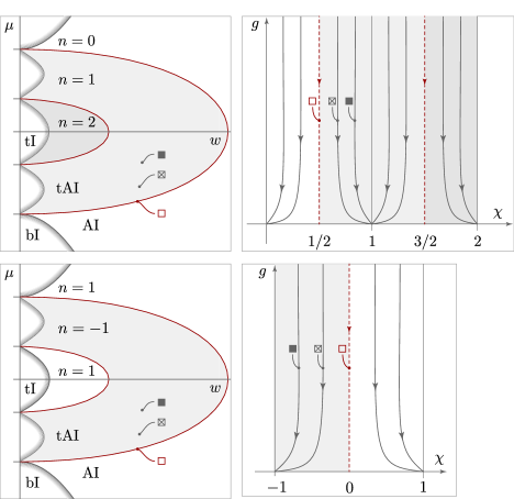
Figure 1: Schematic phase diagram of topological insulators. The $\mathbb{Z}$ (top) or $\mathbb{Z}_{2}$ (bottom) valued topological number of a clean topological insulator can be controlled by a parameter $\mu$ (e.g. chemical potential, magnetic field, etc.). At the transition points separating distinct phases, band gaps close. Disorder, characterized by its strength $w$, induces a crossover from a clean band to an Anderson insulator (shaded lines). The amount of disorder required to close the band gap vanishes at the transition points. The transition points themselves become end points of transition lines in the $(\mu,w)$ phase plane. Driving the system through one of these lines via a parameter change implies IQH type transition with a divergent localization length. The right panels show the flow of the average topological number, $\chi$, and the conductance, $g$ upon increasing the system size, $L$, starting from some non-universal bare values $(\tilde{g},\tilde{\chi})$, defined at a scale of the order of the mean-free path. In the $L\to\infty$ limit, the insulating, $g=0$, and self averaging, $\chi=n$, Anderson topological insulator configurations are generically approached. The critical surfaces separating these regions are characterized by half integer $\chi=n+1/2$ ($\mathbb{Z}$) or vanishing $\chi=0$ ($\mathbb{Z}_{2}$) values of the average topological number.

The high degree of universality reflected in the above can be understood from a simple argument first formulated in Ref. [Motrunich et al., 2001] (cf. Fig. 1): consider a schematic phase plane of a topological insulator spanned by a parameter $\mu$ controlling the topological sector of the system (the chemical potential, a magnetic field, etc.), and a parameter $w$ quantifying the amount of disorder. In the clean system, $w=0$, the topological number jumps at certain values of $\mu$ through topological phase transition points, characterized by a closure of bulk band gaps. Turning on disorder at a generic value of $\mu$ generates a crossover from the clean band insulator into a configuration characterized by a non-vanishing density of states. In most symmetry classes — for the discussion of exceptional situations, see below — Anderson localization will turn the ensuing ‘impurity metal’ into an Anderson insulator. The amount of disorder required to drive this crossover vanishes at the clean system’s gap closing points. At the same time, the closing points mark points of quantum phase transitions and the integrity of these cannot be compromised by the crossover from the band– into the Anderson insulator regime. They become, rather, endpoints of phase transition lines meandering through the phase plane $(\mu,w)$. It is the existence of these lines that distinguishes the ‘topological Anderson insulator’ (tAI) from a conventional Anderson insulator. At the phase transition lines the localization length diverges and the system builds up a delocalized state. From an edge-oriented perspective, the delocalization accompanying a transition $n\to n-1$ means that a pair of edge states is hybridized across the bulk via a delocalized state to disappear (i.e. move away from the zero energy level). Somewhat counter-intuitively, the delocalization phenomenon can be driven by increasing the amount of disorder in the system, or by changing any other parameter capable of changing the system’s location in the phase plane. In early worksBrouwer et al. (1998, 2000a, 2000b) delocalization was observed as a consequence of an ‘accidental’ crossings of phase transition lines. For other crossing protocols see Refs. [Groth et al., 2009; Rieder et al., 2013]. Notice that each phase lobe in Fig. 1 is characterized by an integer invariant. However, the integerness of that value is tied to the limit of infinite system size characterizing a thermodynamic phase. By contrast, the finite size system will generally be described by a non-integer mean topological number, which leads to perhaps counter-intuitive conclusion that Anderson localization actually stabilizes the topological rigidity of disordered systems. The corresponding flow $g\to 0$ (localization) and $\chi\to n$ (re-entrance of the topological number) is described by the two-parameter flow diagram.

For two-dimensional topological insulators the above argument has been made quantitative, to varying degrees of completeness. In some cases (the class A IQH, or the class AII quantum spin Hall effect) no rigorous theory describing the strong coupling regime close to the fixed point exists, but the global pattern of the flow can be convincingly deduced from a two-parameter effective field theory pioneered by PruiskenPruisken (1984) and Fu and KaneFu and Kane (2012), respectively. In the class D or DIII system even the phase diagram is not fully understood, while the exact equivalence of the class C insulator to a percolation problemGruzberg et al. (1999) implies existence of exact solutions for the flow. Remarkably, in two-dimensional systems of chiral symmetry classes AIII, CII and BDI, which are not tI in 2d, the mechanism of Anderson localization is also controlled by the point-like topological defectsKönig et al. (2012) (vortices) and in this way is analogous to class AII topological insulator studied by Fu and Kane.

In this paper, we will focus on the five families of topological multi-channel quantum wires, AIII, CII, BDI, D, DIII. There are far reaching parallels between disordered insulators in one and two dimensions: both show two-parameter scaling, and can be described in terms of field theories — non-linear $\sigma$-models containing a $\theta$-term/fugacity term measuring the action contribution of smooth/point-like topological excitations in the $\mathbb{Z}$/$\mathbb{Z}_{2}$ cases —, the scaling variables are obtained from the field theory via topological sources, and the bulk-boundary correspondence establishes itself by identical mechanisms. However, unlike the 2d systems, the 1d field theories are amenable to powerful transfer matrix techniques. These methods can be applied to solve the problem non-perturbatively, and to describe the results in terms of parameter flows all the way from the diffusive regime into the regime of strong localization. Overall the situation in 1d is similar, but under much tighter theoretical control than in 2d.

II Main results

In this paper we describe five topologically non-trivial insulators in one dimension in terms of supersymmetric nonlinear $\sigma$-models with target spaces representing the different symmetry classes. It provides a framework describing non-translationally invariant topological insulators in terms of a theory that:

• Is universal, in that elements that are not truly essential to the characterization of topological phases, such as translational invariance, or band gaps, do not play a role. The theory, rather, describes the problem in a minimalist way, in terms of symmetry and topology.

• Topological sectors are described in real space, rather than in terms of the more commonly used momentum space homotopy constructions. To this end we study response of supersymmetric partition sum on a twisted boundary conditions. The later are given by a proper gauge transformations dictated by the corresponding symmetry group and containing continuous as well as discrete (i.e. $\mathbb{Z}_{2}$) degrees of freedom.

• These field theories differ from the ones describing conventional Anderson insulators by the presence a topological contribution to the action. The latter weighs the contribution of smooth/point-like topological field excitations in terms of a $\theta$-term/fugacity term depending on whether we are dealing with a $\mathbb{Z}$/$\mathbb{Z}_{2}$ insulator.

• At the bare (short distance) level, the field theories are described by two coupling constants $(\tilde{g},\tilde{\chi})$, where $\tilde{g}$ is the Drude conductance, central to the one-parameter scaling approach to conventional disordered conductors, and $\tilde{\chi}$ is the ensemble average topological number. In the construction of the effective field theory these parameters are obtained from an underlying microscopic disordered lattice model by a perturbative self-consistent Born approximation (SCBA). We provide numerical verification of this approach, which appears to work well down to $N=3$-channel wires (though the theory is developed in $N\to\infty$ limit).

• At large distance scales, these parameters exhibit the flow (4). Using transfer-matrix approach, we provide the exact quantitative description of this flow, including the strongly localized phase and quantum critical points. For generic $\tilde{\chi}$, the fixed point configuration $(g,\chi)\to(0,n)$ is attained exponentially fast in the length, $L$, of the system. The fixed point value for the critical conductance, $g^{\ast}=0$, but the approach to this configuration is algebraic, $\sim L^{-1/2}$. The vanishing of the mean conductance at criticality is manifestation of large sample-to-sample fluctuations in 1d. In fact, it is knownMathur (1997); Brouwer et al. (1998) that a sub-Ohmic scaling $\sim L^{-1/2}$ signifies the presence of a delocalized state in the system. (Some symmetry classes in 2d (D, AII, DIII) exhibit flow more complicated than that depicted in Fig. 1 in that the critical surface broadens into a metallic phase. We return to the discussion of this point below.)

• The theory describes bulk-boundary correspondence by a universal mechanism. In the fixed points, $(0,n)$, the field theory becomes fully topological in the sense that its standard gradient term is absent. In the $\mathbb{Z}$-cases, the topological terms with integer coefficients become Wess-Zumino terms at the boundary, where they describe $n$ gapless boundary excitations.

• In the $\mathbb{Z}_{2}$ cases the fermionic parts of the $\sigma$-model target spaces contain two disconnected componentsBocquet et al. (2000). The topological quantum criticality turns out to be associated with the field configurations with kinks, switching between the two. The corresponding transfer-matrix evolution equation acquires a spinor form, which reveals a hidden supersymmetry (not related to Efetov’s supersymmetry of the underlying $\sigma$-models). Its fermionic degree of freedom, creating kinks between the two sub-manifolds, is dual to the Majorana edge modes, residing on the boundaries between two topologically distinct phases. Such supersymmetry may prove to be crucial for understanding of the bulk-boundary correspondence in the 2d $\mathbb{Z}_{2}$ insulators, which has not yet been worked out.

III Solution strategy

Before delving into more concrete calculations, it is worthwhile to provide an overview of the key elements of our approach to the low energy physics of the five classes of quantum wires:

1. We find it convenient to model our wires as chains of coupled sites, or “quantum dots”, where each site carries an internal Hilbert space accommodating spin indices, multiple transverse channels, etc. The symmetries of the wire and its topological number are encoded in the intra- and inter-site matrix elements describing the system.

2. Disorder is introduced by rendering some of those matrix elements randomly distributed. The choice of those random matrix elements is largely a matter of convenience, i.e. different models of disorder may alter the bare values of the two coupling constants entering the system’s field theory, but not the universal physics.

3. In the clean case, the topological sector of the system can be described in terms of the well established homotopy invariants constructed over the Brillouin zone. We will discuss how this information may be alternatively accessed by probing the response of the spectrum to either extended $(\mathbb{Z})$ or local $(\mathbb{Z}_{2})$ changes in the inter-site hopping. The latter scheme generalizes to the presence of disorder.

4. We describe this response in terms of supersymmetric Gaussian integrals. Upon averaging these integrals over disorder, the symmetries of the microscopic Hamiltonian turn into a ‘dual’ symmetry of the corresponding functional integrals. (The mathematical concept behind this conversion is called ‘Howe-pair duality’ Howe (1989); Cheng and Wang (2012).) In practice this means that the Gaussian actions are invariant under a group $G$ of transformations whose symmetries are in one-to-one correspondence to that of the parent Hamiltonian.

5. If the disorder is strong enough to close the gap, that symmetry gets spontaneously broken to a subgroup $H$. The ensuing Goldstone modes describe diffusive transport in the system. At large distance scales, these modes are expected to “gap out” due to Anderson localization. Within the field theoretical framework, Anderson localization manifests itself in a diminishing of the stiffness of Goldstone modes, and an eventual crossover into a disordered phase, not dissimilar to the disordered phase of a magnet. From yet another perspective one may understand this crossover in terms of a proliferation of topological excitations on the Goldstone mode manifold. At the strong disorder fixed point, which is characterized by a vanishing of longitudinal transport coefficients, the full symmetry of the system, $G$, is restored (once more in analogy to a magnet). However,

6. It remains broken at the boundary points (or lines, in 2d) of the system. As one would expect on general grounds, the boundary Goldstone modes enjoy topological protection and describe the system’s zero energy states.

7. Methodologically, we describe the process of bulk disordering by a method conceptually allied to a real space renormalization group approach. In concrete terms, this means that we map the field integral description onto an equivalent transfer matrix equation which describes the dot-to-dot evolution along the system. The derivation of that equation does not rely on premature field-continuity assumptions. In face, we will observe that in the $\mathbb{Z}_{2}$ cases discontinuous changes of the field play a pivotal role. Evolution via the transfer matrix equation may be understood as a process whereby sites effectively fuse to larger sites, with renormalized parameters. However, rather than describing this process in explicit terms, we will analyze the eigenvalue spectrum of the transfer operator, and from there extract the $L$-dependent flow of observables $(g(L),\chi(L))$.

8. Within the field theoretical framework, the real space topological twists employed to access the system’s topological numbers, become topological field excitations, smooth instantonic configurations/kinks for the $\mathbb{Z}/\mathbb{Z}_{2}$-insulators. The action cost of these configurations is quantified by a topological $\theta$-term/fugacity term. Localization can then be understood in terms of a proliferation of such topological excitations at large distance scales, and this process reflects in an effective flow of both the gradient term, and the coefficient of the topological term. However, at half-integer/zero bare topological coefficient, the contribution of such excitations gets effectively blocked, either in terms of a destructive interference of topological excitations (conceptually similar to what happens in a half-integer antiferromagnetic spin chainHaldane (1983))/or in terms of a vanishing fugacity.

In the rest of the paper, we derive and solve the theory for the five families of topological quantum wires. The presentation is self-contained, however, to keep the main text reasonably compact, details are relegated to appendices. We start out with a preamble (section III), in which we formulate the general strategy of our derivation. To avoid repetitions, we discuss two cases in more detail, viz. the AIII $\mathbb{Z}$-insulator, section IV, and the class D $\mathbb{Z}_{2}$ insulator, section V.3. The theory for the remaining classes, BDI, CII, and DIII, largely parallels that of those two, and will be discussed in more sketchy terms.

IV $\mathbb{Z}$-Insulators

In this section, we derive and analyze the effective theory for the one-dimensional $\mathbb{Z}$-insulators. We start by discussing the simplest of these viz. a ‘chiral’ system lacking any other symmetries, class AIII, in a fairly detailed manner. After that we turn to the time reversal invariant chiral system, class BDI, whose theory will be described in more concise terms, emphasizing the differences to the time reversal non-invariant case. The theory of the third $\mathbb{Z}$ representative, CII, does not add qualitatively new structures, and will be mentioned only in passing.

IV.1 Definition of the model

Consider a system of $N$-quantum wires, described by the Hamiltonian

$$H=\sum\limits_{s=1}^{2L}C^{\dagger}_{s}\left(t_{ss^{\prime}}+R_{ss^{\prime}}\right)C_{s^{\prime}},$$ (5)

where $s$ is a site index, $C_{s}=\{C_{s}^{k}\}$, $k=1,\dots,N$ a vector of $N$ fermion creation operators, and $t$ a nearest neighbor hopping matrix defined through $t_{s,s+1}=t_{s+1,s}=\mu$ if $s$ is even, $t_{s,s+1}=t_{s+1,s}=t$ if $s$ is odd, and zero otherwise, cf. Fig. 2. In other words, the matrix $t$ implements a staggered nearest neighbor hopping chain as realized, e.g., in a Su-Shrieffer-Heeger modelSu et al. (1979). Randomness is introduced into the system through the Hermitean bond random matrices $R_{ss^{\prime}}$ as

$$\left\langle R^{kk^{\prime}}_{s,s^{\prime}}\right\rangle=0,\qquad\left\langle R^{kk^{\prime}}_{s,s+1}R^{k^{\prime}k}_{s+1,s}\right\rangle = \frac{w^{2}}{N},$$ (6)

where all other second moments of matrix elements vanish. To keep the model simple, neighboring chains are only coupled through randomness (one may switch on non-random hopping, at the expense of slightly more complicated formulae).

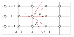
Figure 2: Schematic of a multi-channel AIII quantum wire with staggered hopping of strength $t$, $\mu$, respectively, and random inter-chain hopping described by matrix elements $R^{kk^{\prime}}_{ss+1}$.

To describe the symmetries of the system, we define the site parity operator, $P_{s,s^{\prime}}=(-)^{s}\delta_{ss^{\prime}}$. The fact that the first quantized Hamiltonian $H\equiv t+R$, defined through Eq. (5), is purely nearest neighbor in $s$-space is then expressed by the anti-commutation relation $\{H,P\}_{+}=0$. The absence of other anti-unitary symmetries makes $H$ a member of the chiral symmetry class AIII. To conveniently handle the symmetry of the Hamiltonian, we switch to a two-site unit cell notation through $c_{2s}\to c_{+,s}$, and $c_{2s-1}\to c_{-,s}$. In this representation the Hamiltonian assumes a $+/-$ off-diagonal form, $H=\left(\begin{smallmatrix}&h\cr h^{\dagger}&\end{smallmatrix}\right)$, and $P=\sigma_{3}$ is represented by the Pauli matrix. Anti-commutativity with $P$ implies the symmetry of $H$ under the continuous but transformation $H=THT$, where $T=\exp(i\theta P)$, and $\theta$ is, in general, complex parameter.

IV.2 Topological invariants

In the clean system ($R=0$), one may access the system’s topological invariant by the standardBernevig and Hughes (2013) winding number construction. Turning to a Fourier representation with a wavenumber $q$ conjugate to $s$, the block matrices $h$ become functions $h_{kk^{\prime}}(q)=\delta_{kk^{\prime}}(\mu+te^{iq})$. We then obtain the topological number $n$ as

$$n=\frac{1}{2\pi}\mathrm{Im}\int\limits_{0}^{2\pi}\!dq\,\,\mathrm{tr}(h^{-1}(q)\partial_{q}h(q)).$$ (7)

For the simple model under consideration this becomes $n=N\Theta(|t|-|\mu|)$, where $\Theta$ is the step function. A transverse coupling between the chains would lift the degeneracy of this expression and turn $n$ into a function stepwise diminishing from $N$ to $0$ upon changing system parameters.

We aim to access the number $n$ in a manner not tied to the momentum space. To this end, we consider a system of $L$ unit cells, and close it to form a ring. On this ring, we impose the non-unitary axial transformation $H_{\phi}=T_{\phi}HT_{\phi}$, where $(T_{\phi})_{s,s^{\prime}}=\exp(-i\frac{s}{L}\phi P_{s,s^{\prime}}\delta_{ss^{\prime}})$. The transformation $T_{\phi}$ changes the Hilbert space of the problem, and hence may affect its spectrum. We will show that the sensitivity of the spectrum probes topological sectors. To this end, we notice that the transformation affects the functions $h$ as $h_{kk^{\prime}}(q)\to h_{kk^{\prime}}(q+\phi/L)$ and $h^{\dagger}_{kk^{\prime}}(q)\to h^{\dagger}_{kk^{\prime}}(q-\phi/L)$. We next define the zero energy retarded Green function $G_{\phi}=(i0-H_{\phi})^{-1}$ and compute its sensitivity to the insertion of the flux as

$$\frac{1}{4\pi}\,\ln\left(\frac{\det(G_{2\pi})}{\det(G_{0})}\right)=\frac{1}{4\pi}\int_{0}^{2\pi}d\phi\,\partial_{\phi}\,\mathrm{tr}\ln(G_{\phi})=$$

$$=\frac{1}{4\pi}\,\sum_{q}\int_{0}^{2\pi}\!\!\!d\phi\,\partial_{\phi}\,\mathrm{tr}\left(\ln h(q+\frac{\phi}{L})+\ln h^{\dagger}(q-\frac{\phi}{L})\right)$$

$$=\frac{i}{2\pi L}\mathrm{Im}\sum_{q}\int_{0}^{2\pi}d\phi\,\partial_{q}\,\mathrm{tr}\left(\ln h(q+\phi/L)\right)=$$ (8)

$$=\frac{i}{2\pi}\mathrm{Im}\int_{0}^{2\pi}dq\,\partial_{q}\,\mathrm{tr}\left(\ln h(q)\right),$$ (9)

where in the last line the general identity, $\sum_{q}\int_{0}^{2\pi}d\phi\,F(q+\phi/L)=L\int dqF(q)$ was used. Comparison with Eq. (7) then shows that

$$\frac{1}{4\pi}\mathrm{Im}\ln\left(\frac{\det(G_{2\pi})}{\det(G_{0})}\right)=n.$$ (10)

This equation represents the topological invariant in terms of the ‘spectral flow’ upon insertion of one $2\pi$-twist under the axial transformation. To conveniently compute this expression, we define the “partition sum”,

$$Z(\phi)\equiv\left\langle\frac{\det(G_{\phi_{1}}^{-1})}{\det(G_{-i\phi_{0}}^{-1})}\right\rangle,$$ (11)

where $\phi\equiv(-i\phi_{0},\phi_{1})^{T}$, and following Refs. [Nazarov, 1994; Lamacraft et al., 2004] consider the generating function

$${\cal F}(\varphi_{0})=\partial_{\phi_{1}}Z(\phi)\bigl{|}_{\phi_{1}=-i\phi_{0}}=\partial_{\varphi_{1}}\ln\det(G_{\varphi_{1}})\bigl{|}_{\phi_{1}=-i\phi_{0}},$$ (12)

which contains the full information about the transport properties of the system. From ${\cal F}$, our two variables of interest, $(g,\chi)$ can be accessed,

$$\chi=\frac{1}{4\pi}\int_{0}^{2\pi}d\phi_{1}\,\mathrm{Im}\,{\cal F}(i\phi_{1});\qquad g=-i\partial_{\varphi_{0}}{\cal F}(\varphi_{0})\bigl{|}_{\varphi_{0}=0}.$$ (13)

Here, the second equality expresses the conductance of the system in terms of its sensitivity to a change in boundary conditions. The equivalence of this relation to the linear response representation of the conductance is shown in Sec. VI.

IV.3 Field theory representation

We proceed by representing the ratio of determinants in (11) as a supersymmetric Gaussian integral,

$$Z(\phi)=\left\langle\int d(\bar{\psi},\psi)\,e^{i\bar{\psi}G_{\phi}^{-1}\psi}\right\rangle,$$ (14)

where $\psi=(\psi^{\rm b},\psi^{\rm f})$ and $\psi^{\alpha}$ are vectors of complex commuting ($\alpha=\mathrm{b}$) or Grassmann variables ($\alpha=\mathrm{f}$) with components $\psi^{\alpha}=\{\psi^{\alpha}_{\pm,s,k}\}$. Further $\bar{\psi}^{\mathrm{b}}=\psi^{\mathrm{b}\dagger}$, while $\bar{\psi}^{\mathrm{f}}$ and $\psi^{\mathrm{f}}$ are independent, and $G^{-1}(\phi)\equiv\mathrm{bdiag}(G_{-i\phi_{0}}^{-1},G_{\phi_{1}}^{-1})$ is a block operator in bf-space. Gaussian integration over the super-field $\psi^{\mathrm{b}/\mathrm{f}}$ produces the determinant/inverse determinant of $G_{\phi_{1}}^{-1}/G_{-i\phi_{0}}^{-1}$, and in this way we obtain the partition sum $Z(\phi)$, Eq. (11).

The functional integral possesses a continuous symmetry under transformations

$$\bar{\psi}_{+}\to\bar{\psi}_{+}T_{\mathrm{L}}, \quad\psi_{+}\to T_{\mathrm{R}}^{-1}\psi_{+}$$ (15)

$$\bar{\psi}_{-}\to\bar{\psi}_{-}T_{\mathrm{R}}, \quad\psi_{-}\to T_{\mathrm{L}}^{-1}\psi_{-},$$ (16)

where $T_{\mathrm{L},R}$ are $2\times 2$ supermatrices whose internal structure will be detailed below. A symmetry transformation of this type generally spoils the adjointness relation $\bar{\psi}^{\mathrm{b}}=\psi^{\mathrm{b}\dagger}$, but as long as we make sure not to hit singularities it does not alter the result of the integration.

Denoting the set of these matrices by $\mathrm{GL}(1|1)$, we observe that the action has a continuous symmetry under $G\equiv\mathrm{GL}(1|1)\times\mathrm{GL}(1|1)$. This symmetry may be interpreted as the supersymmetric generalization of the $\mathrm{GL}(n)\times\mathrm{GL}(n)$ symmetry under unitary transformations of left- and right- propagating excitations in chiral quantum systems; it is a direct heritage of the chiral symmetry of the Hamiltonian.

Finally, notice that we may interpret the insertion of the chiral flux $\phi$ in terms of a boundary condition changing chiral gauge transformation, $\bar{\psi}G_{\phi}^{-1}\psi=\bar{\psi}^{\prime}G^{-1}_{0}\psi^{\prime}$, where $\psi^{\prime}_{\mathrm{L/R},s}\equiv e^{(+/-)i\phi\frac{s}{L}}\psi_{\mathrm{L/R},s}$ are subject to the twisted boundary condition $\psi_{\mathrm{L/R},L}^{\prime}=e^{(+/-)i\phi}\psi_{\mathrm{L/R},0}^{\prime}$, where $\phi=\mathrm{diag}(-i\phi_{0},\phi_{1})^{T}$.

IV.4 Disorder average and low energy field theory

We next average the theory over the distribution of the $R$-matrices and from there derive an effective theory describing the physics at distance scales larger than the elastic mean free path. There are two ways of achieving this goalAltland and Merkt (2001), one being explicit construction, the other symmetry reasoning. For an outline of the former route, we refer to Appendix A. Here, we discuss the less explicit, but perhaps more revealing second approach.

The averaging over disorder turns the infinitesimal increment $i0\to i/2\tau$ of the retarded Green function into a finite constant, which defines the inverse of the elastic scattering time. Its value may be exponentially small or not, depending on whether the amplitude of the disorder, $w$, exceeds the gap $\sim|t-\mu|$ of the clean system or not. This criterion defines the crossover from the band insulator into the impurity ‘metal’. The metallic regime is characterized by a globally non-vanishing density of states, and finite electric conduction at length scales shorter than the localization length to be discussed momentarily. In the metallic regime, the appearance of a finite diagonal term $i0\to i/2\tau$ in $\pm$-space ‘spontaneously breaks’ the symmetry under $G$ down to the diagonal group $H=\mathrm{GL}(1|1)$ defined by the equality $T_{L}=T_{R}$. (Within the context of QCD this mechanism is known as the spontaneous breaking of chiral symmetry by gauge field fluctuations, where in our context the role of the latter is played by impurity potential fluctuations.) We expect the appearance of a Goldstone mode manifold, $G/H=(\mathrm{GL}(1|1)\times\mathrm{GL}(1|1))/\mathrm{GL}(1|1)\simeq\mathrm{GL}(1|1)$. In mathematical terminology, that manifold is understood as a Riemannian (super-)symmetric space, viz. the space A$|$A of rank 1. The assignment AIII${}_{\text{Hamiltonian}}\to$ (A$|$A)${}_{\text{field theory}}$ is an example of the symmetry duality mentioned in section III.

We next identify the low energy ‘Ginzburg-Landau’ action $S[T]$ describing the Goldstone mode fluctuations, and its connection to physical observables. Technically (cf. Appendix A.1), the field $T=\{T_{s}\}$ appears after averaging the theory over disorder and decoupling the ensuing $\psi^{4}$-term through a Hubbard-Stratonovich transformation. After integrating over the $\psi$-fields, the partition function then assumes the form ${Z(\phi)=\int{\cal D}T\,\exp(-\tilde{S}[T])}$, where

$$\tilde{S}[T]=\mathrm{str}\ln\left(\begin{matrix}i\Sigma_{0}T&-h\crcr-h^{\dagger}&i\Sigma_{0}T^{-1}\end{matrix}\right),$$ (17)

$\Sigma_{0}=1/2\tau$ is the impurity self-energy evaluated in the self-consistent Born approximation (SCBA) and $h$ contains the disorder independent nearest neighbor hopping matrix elements. Here $\mathrm{str}(A)=\sum_{\alpha}(-)^{\alpha}A^{\alpha\alpha}$ is the so-called supertrace. We recall that the action must be symmetric under the action of the full symmetry group $G$. Within the present context, the latter acts by transformation $T\mapsto T_{L}TT_{R}^{-1}$, i.e. for constant (i.e. $s$-independent) transformations our action must be invariant under independent left- and right-transformation, and the fulfillment of this criterion is readily verified from the structure of the action. Specifically, the action of a constant field $T$ vanishes, $\tilde{S}[T]=\tilde{S}[\mathbb{I}]=0$. To obtain an effective action of soft fluctuations, varying on length scales larger than the lattice constant, we replace the site index $s\to x$ by a continuous variable, $x$, and think of the hopping operators as derivatives. Up to the level of two gradients, two operators can be constructed from field configurations $T_{s}\to T(x)$: $\mathrm{str}(\partial_{x}T\partial_{x}T^{-1})$, and $\mathrm{str}(T^{-1}\partial_{x}T)$. A substitution of $T(x)$ into Eq. (17) followed by a straightforward expansion of the logarithm (cf. Appendix A.1) indeed produces the effective action Altland and Merkt (2001)

$$S[T]=\!\int\limits_{0}^{L}dx\left[-\frac{\tilde{\xi}}{4}\,\mathrm{str}(\partial_{x}T\partial_{x}T^{-1})+\tilde{\chi}\,\mathrm{str}(T^{-1}\partial_{x}T)\right],$$ (18)

where $(\tilde{\xi},\tilde{\chi})$ are two coupling constants. In this expression, the presence of the source variable $\phi$ implies a twisted boundary condition,

$$T(L)=e^{i\phi}T(0)e^{i\phi}.$$ (19)

To make progress, we parameterize the fields $T$ as as $T=U\left(\begin{smallmatrix}e^{y_{0}}&\crcr&e^{iy_{1}}\end{smallmatrix}\right)U^{-1}$, where $U=\exp\left(\begin{smallmatrix}&\nu\crcr\mu&\end{smallmatrix}\right)$ contains the Grassmann variables. The two radial coordinates $(y_{0},y_{1})$ (one non-compact and one compact) parameterize the maximal domain for which the path integral over $T$ with the action (18) is convergent. Notice that the first derivative term, $\mathrm{str}(T^{-1}\partial_{x}T)=\partial_{x}\,\mathrm{str}(\ln T)$ can formally (more on this point below) be expressed as a surface term, indicating that it is a topological $\theta$-term. In the absence of a boundary twist explicitly breaking the symmetry between fermionic and bosonic integration variables, that is for $\phi_{1}=i\phi_{0}$, the functional integral equals unity by supersymmetryEfetov (1997), and $Z(\phi)=1$ by definition, i.e. the connection between $Z(\phi)$ and the functional integral does not include normalization factors.

The interpretation of the two coupling constants $(\tilde{\xi},\tilde{\chi})$ appearing in the action can be revealed by taking a look at the short system size limit $l<L<\tilde{\xi}$, where $l\sim t\tau$ is a short-distance cutoff set by the elastic mean free path due to disorder scattering. In this limit, field fluctuations are suppressed and we may approach the functional integral by stationary phase methods. A straightforward variation of the action $\delta_{T}S[T]=0$ yields the equation $\partial_{x}(T\partial_{x}T^{-1})$, and the minimal solution consistent with the boundary conditions is given by $T_{s}=e^{i2\phi\frac{s}{L}}$. Substituting this expression into the action and ignoring quadratic fluctuations, we obtain the estimate, $Z(\phi)\simeq\exp\left(-\frac{\tilde{\xi}}{L}(\phi_{0}^{2}+\phi_{1}^{2})-2\tilde{\chi}(\phi_{0}-i\phi_{1})\right)$. Application of Eq. (13) then readily yields $\tilde{\chi}=\chi$ and $g=2\tilde{\xi}/L$. This identifies $\tilde{\chi}$ as the bare value of the average topological number, and $\tilde{\xi}$ as the localization length (for $L<\tilde{\xi}$, the conductance of the wire is Ohmic, $g\sim\tilde{\xi}/L$). Within the explicit construction of the theory outlined in Appendix A.1, the coefficients ($\tilde{\xi},\tilde{\chi}$) are obtained as functions of the microscopic model parameters. For the specific model under consideration one finds $\tilde{\xi}=Nl$, and $\tilde{\chi}=\frac{i}{2}\mathrm{tr}(G^{+}P\partial_{k}H)$, where $G^{+}$ is the Green function subject to the replacement $i0\to i/2\tau$. In parentheses we note that this expression can be identified with the expectation value of velocity, or a ‘persistent current’ flowing in response to the axial twist of boundary conditions. Within our present model, one obtains $\tilde{\chi}=\frac{N}{2}(1+\frac{(t-\mu)t}{w^{2}})$, see Appendix A.1 for more details.

IV.5 Anderson localization

Before exploring in quantitative terms what happens at large scales, $L>\tilde{\xi}$, let us summarize some anticipations. For generic values of $\tilde{\chi}$ one expects flow into a ‘disordered’ regime. At large distance scales, the fields exhibit strong fluctuations and the ‘stiffness’ term $\propto\tilde{\xi}$ becomes ineffective. (Within an RG oriented way of thinking, one may interpret this as a scaling of a renormalized localization length $\xi(L)\to 0$.) On general grounds, we expect this scaling to be accompanied by a scaling $\chi(L)\to n$. At the fixed point, the Goldstone modes disappear from the bulk action, which we may interpret as a restoration of the full chiral group symmetry $G$. The presence/absence of this symmetry is a hallmark of localized/metallic behavior, the scaling is towards an attractive bulk insulating fixed point.

As for the boundary, the fixed point topological term with quantized coefficient $n\int dx\,\mathrm{str}(T^{-1}\partial_{x}T)=n\,\left[\mathrm{str}\ln(T(L))-\mathrm{str}\ln(T(0))\right]\equiv S_{\mathrm{b}}[T]$, becomes a surface term, where we temporarily assume our system to be cut open. For generic values $\chi\not=n$ it actually is not a surface term, because $T=T(y_{0},y_{1})=T(y_{0},y_{1}+2\pi)$ is $2\pi$-periodic in the coordinates $y_{1}$ while $\exp(-\chi\,\mathrm{str}\ln T)=\exp(-\chi(y_{0}-iy_{1}))$ is not. The requirement of a quantized coefficient reveals the surface terms $n\,\mathrm{str}\ln T$ as zero dimensional variant of Wess-Zumino term. At any rate, the $G$-symmetry at the boundary remains broken, and we will discuss in section IV.6 how this manifests itself in the presence of protected surface states. Notice how the protection of these states is inseparably linked to bulk localization. The latter plays the role of the bulk band gap in clean systems.

The above picture can be made quantitative by passing from the functional integral to an equivalent “transfer matrix equation”Efetov (1997); Altland and Merkt (2001). The latter plays a role analogous to that of the Schrödinger equation of a path integral. Interpreting length as (imaginary) time, it describes how the amplitude $\Psi(\phi,L)\equiv Z(\phi,L)-1$ defined by the functional integral at fixed initial and final configuration $T(0)=\mathds{1}$, $T(L)=\exp(2i\phi)$ evolves upon increasing $L$. (Since $Z(0,L)=1$, by its supersymmetric normalization the function $\Psi$ is defined to describe the non-trivial content of the partition sum.) This equation, whose derivation is detailed in Ref. [Altland and Merkt, 2001], is given by

$$-\tilde{\xi}\,\partial_{x}\Psi(y,x)=\frac{1}{J(y)}(\partial_{\nu}-iA_{\nu})J(y)(\partial_{\nu}-iA_{\nu})\Psi(y,x),$$ (20)

where ${J(y)=\sinh^{-2}\left(\frac{1}{2}(y_{0}-iy_{1})\right)}$ is the Jacobian of the transformation to the radial coordinates $y_{\nu}$, $\partial_{\nu}=\partial/\partial_{y_{\nu}}$, $A_{\nu}=\tilde{\chi}\,i^{1-\nu}$, and the index $\nu=0,1$ is summed over. To understand the structure of this equation notice that the action of the path integral (18) resembles the Lagrangian of a free particle, subject to a constant magnetic field. One therefore expects the corresponding transfer matrix equation to be governed by the Laplacian on the configuration space manifold $\mathrm{GL}(1|1)$ of the problem. The differential operator appearing in Eq. (20) is the radial part of that Laplacian (much like $r^{-2}\partial_{r}r^{2}\partial_{r}$ is the radial part of the Laplacian in spherical coordinates), i.e. the contribution to the Laplacian differentiating invariant under angular transformations $U$. The presence of the Jacobian $J(y)$ reflects the non-cartesian metric of the manifold, and the vector potential, $A_{\nu}$, is proportional to the bare topological parameter $\tilde{\chi}$.

It is straightforward to identify the eigenfunctions and eigenvalues of the transfer matrix operator as

$$\psi_{l}(y) =\sinh\left(\frac{1}{2}(y_{0}-iy_{1})\right)e^{il_{\nu}y_{\nu}},$$ (21)

$$\epsilon(l)=(l_{0}-i\tilde{\chi})^{2}+(l_{1}-\tilde{\chi})^{2},$$ (22)

where $l_{0}\in\mathbb{R}$, and $l_{1}\in\mathbb{Z}+\frac{1}{2}$ to make the eigenfunctions $2\pi$-periodic in $\tilde{y}_{1}$. We may now employ these functions to construct a spectral decomposition $\Psi(\phi,L)=\sum_{l_{1}}\int dl_{0}\,\mu(l)\,\psi_{l}(\phi)e^{-\epsilon(l)L/\tilde{\xi}}$. Using that

$$\left\langle\psi_{l},\psi_{l^{\prime}}\right\rangle \equiv\int\limits_{0}^{\infty}dy\int\limits_{0}^{2\pi}d\tilde{y}\,J(y)\bar{\psi}_{l}(y)\psi_{l^{\prime}}(y)=$$ (23)

$$\quad=(2\pi)^{2}\delta(l_{0}-l_{0}^{\prime})\delta_{l_{1}l^{\prime}_{1}},$$ (24)

it is straightforward to obtain the expansion coefficients $\mu(l)$ by taking the scalar product $\left\langle\psi_{l},\Psi(L\to 0)\right\rangle$. Upon substitution of the limiting value $\Psi(\phi,L\to 0)\rightarrow-1$ (at any $\phi$, but $\phi=0$, where $\Psi(\phi,L\to 0)\rightarrow 0$) , we obtain $\mu(l)=\frac{1}{\pi}\frac{1}{l_{1}+il_{0}}$ and thus

$$Z(\phi)=1+\sum_{l_{1}\in\mathbb{Z}+\frac{1}{2}}\int\frac{dl_{0}}{\pi}\,\frac{\psi_{l}(\phi)}{l_{1}+il_{0}}\,e^{-\epsilon(l)L/\tilde{\xi}}.$$ (25)

Differentiation of this result, according to Eq. (13), yields the two observables of interestAltland et al. (2014)

$$g = \sqrt{\frac{\tilde{\xi}}{\pi L}}\sum_{l_{1}\in\mathbb{Z}+1/2}e^{-(l_{1}-\tilde{\chi})^{2}L/\tilde{\xi}},$$ (26)

$$\chi = n-\frac{1}{4}\!\sum_{l_{1}\in\mathbb{Z}+1/2}\!\left[\mathrm{erf}\Big{(}\sqrt{\frac{L}{\tilde{\xi}}}\,(l_{1}-\delta\tilde{\chi})\Big{)}-(\delta\tilde{\chi}\leftrightarrow-\delta\tilde{\chi})\right],$$

where $\delta\tilde{\chi}=\tilde{\chi}-n$ is the deviation of $\tilde{\chi}$ off the nearest integer value, $n$.

These equations quantitatively describe the scaling behavior anticipated on qualitative grounds above: for generic bare values $(\tilde{\xi},\tilde{\chi})$ we obtain an exponentially fast flow of $(g(L),\chi(L))$ towards an insulating state $(0,n)$. At criticality, $(\tilde{\xi},n+1/2)$, the topological number remains invariant, while algebraic decay of the conductance $g(L)\approx\sqrt{\tilde{\xi}/\pi L}$ indicates the presence of a delocalized state at zero energy (i.e. in the center of the gap of a clean system). Introducing the scaling form $\xi(\tilde{\chi})=\tilde{\xi}|\tilde{\chi}-n-1/2|^{-\nu}$ and comparing the ansatz, $g\sim\exp(-L/\xi(\tilde{\chi}))$, with the result above, we obtain the correlation length exponent $\nu=2$ describing the exponential decay of the average conductance, $\langle g\rangle$. (This exponent differs from ${\nu=1}$ for the typical correlation length, ${\left\langle\xi\right\rangle}=-L/\langle\ln g\rangle$.Brouwer et al. (1998); Mondragon-Shem et al. (2014)) The flow is shown graphically in Fig. 3, and it represents the 1d analogue of the two-parameter flow diagram Khmelnitskii (1983) describing criticality in the integer QH system.

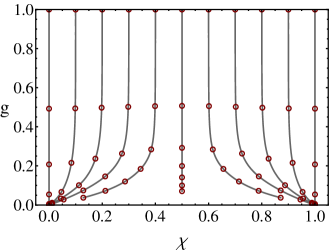
Figure 3: Flow of the conductance $g$ and the topological parameter $\chi$ as a function of system size for class AIII system. Dots are for values, $L/\tilde{\xi}=1,2,4\dots,32$.

In Fig. 4 we show the phase diagram of $N=3$–channel disordered AIII wire in the $(\mu,w)$ plane. The clean system, $w=0$, exhibits topological phase transitions at $\mu/t=\pm 1$. Solid lines show half-integer values of the SCBA computed topological number $\tilde{\chi}$, see Appendix A.1 for the details. Squares show numerically computedAltland et al. (2014) boundaries between regions with different number of negative Lyapunov exponents, section VI, of the transfer matrix. Notice a very satisfactory agreement between numerical transfer-matrix calculation and SCBA, even though the latter is justified only in $N\gg 1$ limit.

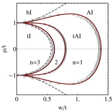
Figure 4: Phase diagram of the $\mathrm{AIII}$ class 3-channel disordered wire. Dashed lines show crossover regions between band insulator (bI) and Anderson insulator (AI) or tI and tAI phases, derived from the SCBA. Solid lines correspond to half-integer values of the SCBA computed topological number $\tilde{\chi}$ and mark boundaries between phases of different $n$. bI and AI have $n=0$, while for tI and tAI $n\neq 0$. Squares: data points, representing phase boundaries found from a numerical analysis of Lyapunov exponents, section VI.

.

IV.6 Density of states

The critical physics discussed above also shows in the density of states of the system. We here recapitulate a few results derived in more detail in Ref. [Altland and Merkt, 2001]. At the insulating fixed points, $(0,n)$, the zero energy action of the system with vacuum boundary conditions reduces to the boundary action $S_{\mathrm{b}}[T]$, i.e. the $G$-symmetry remains broken at the metallic system boundaries, which may be interpreted as ‘quantum dots’ of size $\simeq\tilde{\xi}$. At finite energies, $E$, the boundary action representing the Green function $G_{E}\equiv(E+i0-H)^{-1}$ at, say, the left boundary is given byIvanov (2002)

$$S_{\mathrm{L}}[T]=-n\,\mathrm{str}(\ln T)+i\frac{\epsilon}{2}\,\mathrm{str}(T+T^{-1}),$$ (27)

where $\epsilon=\pi|E|/\Delta_{\xi}$, and $\Delta_{\xi}$ is the average single particle level spacing of a wire segment of extension $\tilde{\xi}$. The fact that the energy $\epsilon$ enters the action like a ‘mass term’ for the Goldstone modes reflects the explicit breaking of the chiral symmetry $\{G^{-1}_{E},P\}_{+}\not=0$. From this expression, the density of states at the system boundaries is obtained as

$$\rho(\epsilon)=\frac{1}{2\Delta_{\xi}}\left\langle(T+T^{-1})^{\mathrm{bb}}\right\rangle.$$ (28)

The integral can be done in closed form, and as a result one obtainsVerbaarschot and Zahed (1993); Ivanov (2002)

$$\rho(\epsilon)=\frac{1}{\Delta_{\xi}}\left(\pi n\delta(\epsilon)+\frac{\pi\epsilon}{2}\left[J_{n}^{2}(\epsilon)-J_{n+1}(\epsilon)J_{n-1}(\epsilon)\right]\right).$$ (29)

The first term here represents the $n$ topologically protected zero energy states, and the second describes the rest of the spectrum in terms of a bathtub shaped function which remains strongly suppressed up to values $|E|\sim n\Delta_{\xi}$. This suppression reflects the level repulsion off the zero energy states in the chaotic scattering environment provided by the disorder. For larger energies, the second term asymptotes to unity, i.e. $\rho(\epsilon)\stackrel{{\scriptstyle\epsilon\gg 1}}{{\longrightarrow}}\Delta_{\xi}^{-1}$. The boundary DoS obeys the sum rule $\lim_{\Delta\epsilon\to\infty}\int_{-\Delta\epsilon}^{\Delta\epsilon}d\epsilon\,\rho(\epsilon)=2\Delta\epsilon/\Delta_{\xi}$, i.e. the spectral weight $n$ sitting at zero all is taken from the bulk of the spectrum.

At criticality, the bulk of the system remains in a symmetry broken state. The transfer matrix method discussed above may then be applied to compute the bulk density of states (28) at observation points $\xi\ll x\ll L$ deep in the system. The resultAltland and Merkt (2001): $\nu(\epsilon)=-\frac{\nu_{0}}{\epsilon\ln^{3}(\epsilon)}$ shows a strong accumulation of spectral weight at the band center. This spectral anomaly is based on the same buildup of long range correlations that gives rise to the delocalization phenomenon. Heuristically, one may interpret it as a ‘channel’ through which a left and a right boundary state hybridize at the critical point to move away from the zero energy.

IV.7 Topological Sources

Unlike the locally confined source terms commonly used to compute observables from field theories, the phase variable $\phi$ employed above is a ‘topological’ source’, i.e. one that twists boundary conditions and is defined only up to local deformation. In view of our later consideration of other symmetry classes we here briefly discuss the geometric principles behind this construction and how to extract the variable pair $(g,\chi)$ from the field theory by boundary twists generalizing the phase variable $\phi$ to other symmetry classes.

In all one-dimensional cases the relevant fields are ‘maps’ $Q:S^{1}\to G/H$ from a circle (the quantum wire compactified to a ring) into a Goldstone mode manifold realized as the quotient of a full symmetry group $G$ over a group of conserved symmetry $H$, e.g. $G=\mathrm{GL}(1|1)\times\mathrm{GL}(1|1)$ and $H=\mathrm{GL}(1|1)$ above. We are putting quotes in ‘map’ because it is essential to include fields subject to boundary twist, i.e. configurations that cannot be described in terms of smooth maps. Also, in some cases, the Goldstone mode manifold includes a discrete Ising type sector $\sim\mathbb{Z}_{2}$ which is non-smooth by itself. A more geometric way to think of the fields would be in terms of sections of a bundle structure, where the latter has $S^{1}$ as its base, and $G/H$ as fibers. Within this setting, the emergence of boundary twist means that we will be met with ‘nontrivial bundles’, i.e. the ones that cannot be reduced to a product space $S^{1}\times G/H$. This is another way of saying that in the presence of twist there are no globally continuous fields. On the bundle structure, the group $G$ acts as a local symmetry group, e.g. by the transformations $T\to T_{L}TT_{R}^{-1}$, $(T_{L},T_{R})\in G=\mathrm{GL}(1|1)$, which makes our theory a gauge theory. The source fields employed to compute observables are gauge transformations by themselves, and they do cause boundary twist. In more mathematical language, one would say that the bundle is equipped with a non-trivial connection, i.e. a twisted way of parallel transportation. The absence of periodicity on the twisted background can be equivalently described as the presence of non-vanishing curvature or gauge flux. The theory responds to the presence of such type of connection in terms of deviations of the partition sum $Z$ off unity, and in this way the observable pair $(g,\chi)$ can be obtained. The situation bears similarity to the quantum mechanical persistent current problem, where the presence of a magnetic flux (or twisted boundary conditions) leads to flux-dependence of the free energy (corresponding to our $Z$). In that context, the insertion of a full flux quantum generates spectral flow, i.e. a topological response (similar to our $\chi$), while the probing of ‘spectral curvature’, i.e. a second order derivative w.r.t. the flux generates a dissipative response (’Thouless conductance’, similar to our $g$).

The question then presents itself how the connection yielding the observables should be chosen in concrete cases. (In view of the dimensionality $>1$ of the target manifolds there is plenty of freedom in choosing twisted connections, which nevertheless may yield equivalent results.) Below, we will approach this question in pragmatic terms, i.e. we have an expression of the topological invariants in terms of Green functions, these Green functions can be represented in terms of Gaussian superintegrals (cf. Eq. (14)) subject to a source, and that source then lends itself to an interpretation as a gauge field acting in the effective low energy field theory (cf. Eq. (18).) While the concrete implementation of this prescription depends on the symmetry class, and in particular on whether a $\mathbb{Z}$ or a $\mathbb{Z}_{2}$ insulator is considered the general strategy always remains the same. Likewise, the extension of the source formalism to one yielding the dissipative conductance is comparatively straightforward, as discussed in the specific applications below. We finally note that the global gauge formalism can be generalized to higher dimensions, Pruisken’s ‘background field method’Pruisken (1984) being an early example of a $d=2$ implementation. For further discussion of this point see section VII.

IV.8 Class BDI

We next extend our discussion to the one-dimensional $\mathds{Z}$-insulator in the presence of time reversal, symmetry class $\mathrm{BDI}$. Class BDI can be viewed as a time reversal invariant extension of class AIII discussed above. Readers primarily interested in the much more profound differences between $\mathbb{Z}$ and $\mathbb{Z}_{2}$ insulators, are invited to directly proceed to section V

Model Hamiltonian — Systems of this type are realized, e.g. as $N$-channel lattice $p$-wave superconductorsKitaev (2001) with the Hamiltonian

$$H=\sum_{s=1}^{L}[C^{\dagger}_{s}H_{0,s}C_{s}+(C^{\dagger}_{s}H_{1,s}C_{s+1}+\mathrm{h.c.})],$$ (30)

where the spinless fermion operators $C_{s}=(c_{s,k},c_{s,k}^{\dagger})^{T}$ are vectors in channel and Nambu spaces with $s$ being site and $k=1,...,N$ being channel indices. The on-site part of the Hamiltonian, ${H_{0,s}=(\mu+V_{s})\sigma_{3}}$ contains the chemical potential $\mu$ and real symmetric inter-chain matrices $V_{s}^{kk^{\prime}}$. The Pauli matrices $\sigma_{i}$ operate in Nambu space. The inter-site term, $H_{1,s}=-\frac{1}{2}t_{s}\sigma_{3}+\frac{1}{2}\Delta_{s}\sigma_{2}$, contains nearest neighbor hopping, $t_{s}$, and the order parameter, $\Delta_{s}^{kk^{\prime}}$, here assumed to be imaginary for convenience. Quantities carrying a subscript ‘$s$’ may contain site-dependent random contributions. The first quantized representation of $H$ obeys the chiral symmetry $\{P,H\}_{+}=0$, with $P=\sigma_{1}$ and the BdG particle-hole symmetry $\sigma_{1}H^{T}\sigma_{1}=-H$. The combination of these two results in the effective time-reversal symmetry $H^{T}=H$. In what follows we consider the simplest model of disorder in which $t_{s}=\Delta_{s}=t$ are non-random and diagonal in the channel space while the matrices $V_{s}^{kk^{\prime}}$ are Gaussian distributed as

$$\langle V_{s}^{kk^{\prime}}V_{s}^{k^{\prime\prime}k^{\prime\prime\prime}}\rangle=(w^{2}/N)(\delta_{k^{\prime}k^{\prime\prime}}\delta_{kk^{\prime\prime\prime}}+\delta_{kk^{\prime\prime}}\delta_{k^{\prime}k^{\prime\prime\prime}}),$$ (31)

and the parameter $w$ sets the strength of the disorder.

Field theory —

Due to the presence of both chiral and time-reversal symmetry the Goldstone mode manifold of the effective low-energy field theory in the BDI class spans the coset space $\mathrm{GL}(2|2)/\mathrm{OSp}(2|2)$ Zirnbauer (1996) which can be parameterized in terms of $4\times 4$ matrices $Q=T\bar{T}$, where the ’bar’ operation is defined as $\bar{T}=\tau T^{T}\tau^{T}$ and $\tau={\cal P}^{\mathrm{b}}\otimes\tau_{1}+{\cal P}^{\mathrm{f}}\otimes i\tau_{2}$. Here ${\cal P}^{\mathrm{b}}$ and ${\cal P}^{\mathrm{f}}$ are projectors on the bosonic and fermionic space while $\tau$-matrices operate in the so-called ’charge-conjugation’ space. It is clear from this parametrization that all matrices $T$ obeying $\bar{T}=T^{-1}$ form the subgroup $K=\mathrm{OSp}(2|2)$ in the larger group $G=\mathrm{GL}(2|2)$ and do not contribute to the $Q$-field, which thereby spans the coset $G/K$. By considering rotations in the fermionic sector only, one finds that $T_{\rm ff}\in{\rm U}(2)/{\rm Sp}(2)\simeq{\rm U}(1)\simeq S_{1}$. The non-trivial homotopy group $\pi_{1}(S_{1})=\mathds{Z}$ implies the presence of winding numbers in the low-energy field theory.

For our subsequent discussion we will need the parametrization of the Goldstone manifold spanned by 8 coordinates, three of which, $(y_{0},y_{1},y_{2})$ with $y_{0}\in\mathds{R}$, $y_{1}\in[0,2\pi[$, and $y_{2}\in\mathds{R}^{+}$, play the role analogous to the radial coordinates of the $\mathrm{AIII}$ manifold. It reads

$$Q=e^{\cal W}{\cal Q}e^{-{\cal W}},\quad{\cal Q}=\left(\begin{array}[]{cc}{\cal Q}^{\rm bb}&\\ &{\cal Q}^{\rm ff}\end{array}\right)^{\rm bf}$$ (32)

where the ff-block ${\cal Q}^{\rm ff}=e^{2iy_{1}}\tau_{0}$ is parametrized by a compact radial variable $y_{1}$ and the bb-block is parametrized by two hyperbolic radial variables $y_{0,2}$ and one angle $\alpha$,

$${\cal Q}^{\rm bb}=e^{2y_{0}}\times e^{i\alpha\tau_{3}}e^{2y_{2}\tau_{1}}e^{-i\alpha\tau_{3}}.$$ (33)

The off-diagonal rotations mixing bosonic and fermionic sectors have the form

$${\cal W}=\left(\begin{array}[]{cc}&{\cal B}\\ \tilde{\cal B}&\end{array}\right)^{\rm bf},\quad{\cal B}=\left(\begin{array}[]{cc}\xi&\nu\\ \mu&\eta\end{array}\right),$$ (34)

where ${\cal B}$ is a matrix in charge-conjugation space depending solely on Grassmann angles and $\tilde{\cal B}=i\tau_{2}{\cal B}^{T}\tau_{1}$.

The field theory action of the BDI disordered system has the same form as in the class $\mathrm{AIII}$,

$$S[Q]=\!\int\limits_{0}^{L}\!\!dx\left[-\frac{\tilde{\xi}}{16}\,\mathrm{str}(\partial_{x}Q\partial_{x}Q^{-1})+\frac{\tilde{\chi}}{2}\,\mathrm{str}(Q^{-1}\partial_{x}Q)\right],$$ (35)

and a sketch of its derivation is outlined in Appendix A.2. The topological coupling constant is given by $\tilde{\chi}=\frac{i}{2}{\rm tr}(G^{+}P\partial_{k}H)$, where the retarded Green’s function $G^{+}$ has to be calculated within the SCBA. The concrete dependence of $\tilde{\chi}$ on the parameters defining the model (30) will be discussed below.

The ’partition sum’ of the $\mathrm{BDI}$ system is again given be Eq. (11), and its path integral representation reads $Z(\phi)=\int{\cal D}Q\exp(-S[Q])$, where the integral is over all smooth realizations of the $Q$-field with fixed initial and final configuration, $Q(0)=\mathds{1}$ and $Q(L)={\rm diag}(e^{2\phi_{0}},e^{2i\phi_{1}})^{\rm bf}$. As in the $\mathrm{AIII}$ system its non-trivial content $\Psi(\phi,L)\equiv Z(\phi,L)-1$ can be found from the solution of the transfer matrix equation (20), which is now defined for three radial coordinates $y=(y_{0},y_{1},y_{2})$, with Jacobian

$$J(y)=\frac{\sinh(2y_{2})}{16\sinh^{2}(y_{0}-iy_{1}+y_{2})\sinh^{2}(y_{0}-iy_{1}-y_{2})},$$ (36)

and vector potential $A=2\tilde{\chi}(i,1,0)^{T}$. The partition sum is obtained from the solution of the equation at the radial configuration $y=\phi\equiv(\phi_{0},\phi_{1},0)$.

The spectrum of the transfer matrix operator can be found by analyzing the asymptotic of the eigenfunctions $\psi_{l}(y)$ at large values of variable $y_{0,2}$. In this regime the $\sinh$-functions simplify to exponentials and the eigenfunctions $\psi_{l}(y)$ show the same exponential profile. In this way we find

$$\epsilon(l_{0},l_{1},l_{2})=1+(l_{0}-2i\tilde{\chi})^{2}+(l_{1}-2\tilde{\chi})^{2}+l_{2}^{2},$$ (37)

with $l_{1}\in 2\mathds{Z}$ and $l_{0,2}\in\mathds{R}$.

Obtaining the initial value solution $\Psi(\phi,L)$ requires the application of more elaborate techniques. The key is to extend the super-Fourier analysis of Ref. [Mirlin et al., 1994] for the three standard Dyson symmetry classes to the symmetry classes presently under consideration. Relegating an exposition of mathematical details to a subsequent publication, we here state only the main results. For any set of radial coordinates $y=(y_{0},y_{1},y_{2})$ the partition sum can be written as a spectral sum analogous to Eq. (25) for the class $\mathrm{AIII}$ system

$$\Psi(y,L)=\sum_{l_{1}\in 2\mathds{Z}}\int\frac{dl_{0}dl_{2}}{(2\pi)^{2}}\,\mu(l)\psi_{l}(y)e^{-\epsilon(l)L/2\tilde{\xi}}.$$ (38)

Here $l=(l_{0},l_{1},l_{2})$ denotes the set of quantum numbers, and the measure $\mu(l)$ is found to be

$$\mu(l)=\frac{(\pi l_{2}/8)\tanh(\pi l_{2}/2)}{\left[l_{2}^{2}+(il_{0}+l_{1}-1)^{2}\right]\left[l_{2}^{2}+(il_{0}+l_{1}+1)^{2}\right]}.$$ (39)

The functions $\psi_{l}(y)$ appearing in the Fourier expansion (38) are the generalized spherical eigenfunctions of the Laplace-Beltrami operator on the coset space $G/K$. They do not depend on the vector potential $A\sim\tilde{\chi}$. As in the AIII case, the topological parameter enters the solution $\Psi(y,L)$ only through the $\tilde{\chi}$-dependence of the spectrum $\epsilon(l)$, Eq. (37).

While for arbitrary $y$ the wave function $\psi_{l}(y)$ cannot be written in closed form, an integral representation due to Harish-Chandra Helgason (1984) exists. The analysis of this representation greatly simplifies for the configuration of interest, $y=(\phi_{0},\phi_{1},0)$. Using the Harish-Chandra integral representation for $\psi_{l}(\phi)$ we obtain the generating function ${\cal F}(\phi)$, Eq. (12), as

$${\cal F}(\phi)=4\,\partial_{\phi_{1}}\sum_{l_{1}\in 2\mathds{Z}}\int\frac{dl_{0}dl_{2}}{\pi^{2}}\,\mu(l)e^{(il_{1}-l_{0})\phi_{1}}e^{-\epsilon(l)L/2\tilde{\xi}}.$$ (40)

From this result the asymptotic values of $\chi(L)$ and $g(L)$ in the limit $L/\tilde{\xi}\gg 1$ can be extracted, and we obtain results qualitatively similar to those of the $\mathrm{AIII}$ system. For example, far from criticality keeping the dominant terms in the Fourier series (40) we find

$$\chi(L) \simeq n+\frac{1}{4}\,{\rm sign}(\delta\chi)\,\sqrt{\frac{\xi(\tilde{\chi})}{\pi L}}\,e^{-L/\xi(\tilde{\chi})},$$

$$g(L) \simeq \frac{1}{2}\sqrt{\frac{\tilde{\xi}}{\pi L}}\,e^{-L/\xi(\tilde{\chi})},$$ (41)

where as before $\tilde{\chi}=n+\delta\chi$ and the localization length $\xi(\tilde{\chi})=\tilde{\xi}|\tilde{\chi}-n-1/2|^{-2}$.

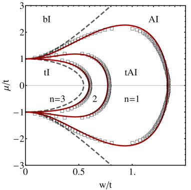
Figure 5: Phase diagram of the $\mathrm{BDI}$ class 3-channel disordered $p$-wave superconducting wire. Dashed lines show crossover regions between band insulator (bI) and Anderson insulator (AI) or tI and tAI phases, derived from the SCBA. Solid lines correspond to half-integer values of the SCBA computed topological number $\tilde{\chi}$ and mark boundaries between phases of different $n$. bI and AI have $n=0$, while for tI and tAI $n\neq 0$.

.

Phase diagram —

For the model of the $N$-channel $p$-wave wire defined above, the constant $\tilde{\chi}=\tilde{\chi}(\mu,w)$ takes values in the interval $(0,N)$. Its explicit form can be found analytically in limiting cases. Specifically, in the low energy limit $|\mu-t|\ll t$ we obtain

$$\tilde{\chi}(w,\mu)=\frac{N}{4}\left(3+\frac{(t-\mu)t}{w^{2}}\right),$$ (42)

while in the limit $\mu\to 0$ and for any disorder strength $w$,

$$\tilde{\chi}(\mu=0,w)=Nt^{2}/2w^{2}.$$ (43)

Localization is avoided if $\tilde{\chi}(\mu,w)=n+1/2$, with integer $n\in[0,N-1]$, and the corresponding contour lines in the $(\mu,w)$-plane define boundaries between different phases of the tAI with indices $n$ and $n+1$. The ensuing phase diagram at $N=3$ is shown in Fig. 5. Using Eq. (43) we find that the phase transition points on the $(\mu=0;w)$ line are located at

$$w_{n}=t(2N/(2n+1))^{1/2},$$ (44)

where $0\leq n<N$ (cf. also Ref.Rieder et al., 2013). Similarly, employing relation (42) we find that the degenerate phase transition point $(\mu,w)=(t;0)$ on the clean system ordinate splits into the set of $N$ critical parabolas

$$\mu_{n}(w)=t+\frac{w^{2}}{t}\left(3-\frac{4n+2}{N}\right).$$ (45)

We have also compared the profiles of the $\chi=n+1/2$ contour lines obtained by SCBA evaluation of the topological parameter against numerical transfer matrix method. The excellent agreement was found, in spite of the fact that strictly speaking the field theory approach requires $N\gg 1$. The diagram in Fig. 5 supports the qualitative discussion of the introductory section. In particular, one observes that somewhat counterintuitively the increase of disorder strength $w$ at fixed chemical potential $\mu$ may induce the quantum phase transition (and thus delocalization!) from the trivial Anderson insulator ($n=0$) to the tAI ($n=1$)Fulga et al. (2011, 2012).

We conclude by noting that the physics of the class CII quantum wire, governed by a chiral time-reversal invariant Hamiltonian, with broken spin-rotation invariance, is essentially similar to that of the AIII and BDI systems. A quantitative solution along the lines of the ones discussed above can be formulated, but it does not add qualitatively new information and we do not discuss it here.

V $\mathbb{Z}_{2}$ insulators

In many ways, the effective theories of the five classes of topological quantum wires resemble each other. All five can be described in terms of two parameter nonlinear $\sigma$-models, and in all cases critical flows characterized by the fixed point structure (4) are predicted. (Similar parallels are observed in 2d, cf. section VII.) However, there are also important differences notably between the $\mathbb{Z}$ and $\mathbb{Z}_{2}$ representatives. The rule of thumb is that while the topological textures responsible for the flow in the $\mathbb{Z}$-insulators are smooth – phase windings in 1d, instantons in 2d – they are singular in the $\mathbb{Z}_{2}$ systems – point defects in 1d, line defects in 2d. The $\mathbb{Z}_{2}$-wires considered below are driven into a localized regime by a proliferation of kinks. Much like vortices in 2d (which have been seenFu and Kane (2012) to play a similar role there), kinks are topological in nature, however they cannot be described in terms of a gradient-topological term. Its role is taken, rather, by a fugacity term, i.e. a term describing the action cost of individual kinks. The fugacity coefficient, $\ln(\tilde{\chi})$ assumes the role of the $\theta$-angle in the $\mathbb{Z}$-insulators.

In the following we describe the construction and solution of the theory on the example of the class D quantum wire, i.e. the spin-rotation and time- reversal symmetry broken system currently under intense experimental and theoretical scrutiny. We then generalize the treatment to class DIII system.

V.1 Definition of the model

The Bogoliubov-deGennes Hamiltonian of class D superconductor obeys the symmetry relation $H^{T}=-\sigma_{1}^{\mathrm{ph}}H\sigma_{1}^{\mathrm{ph}}$, where the Pauli matrices act in particle-hole space. One may perform unitary transformation to ‘real’ superpositions of particle and hole degrees of freedom – the ‘Majorana’ basis – in which the symmetry assumes the simple form $H=-H^{T}$. We will work in this basis throughout, and model our system as a chain of $L$ coupled ‘dots’, $s=1,\dots,L$ where each dot represents a disordered superconductor. The corresponding Hamiltonian reads

$$H=\sum_{ss^{\prime}}C_{s}^{\dagger}\left[{\cal H}_{s}\delta_{ss^{\prime}}+iW(\delta_{ss^{\prime}+1}-\delta_{s^{\prime}s+1})\right]C_{s^{\prime}},$$ (46)

where ${\cal H}_{s}=-{\cal H}_{s}^{T}$ is a matrix ${\cal H}_{s}=\{{\cal H}_{s}^{kk^{\prime}}\}$ with random contributions, and the inter-dot coupling matrices, $W=W^{T}$, are assumed to be non-random. Without loss of generality, we may choose a basis in which $W=\mathrm{diag}(w_{1},\dots,w_{2N})$ is diagonal.

V.2 Topological invariant

In the clean case, the $\mathbb{Z}_{2}$ invariant carried by the system is defined asKitaev (2001) $\mathrm{sgn}\left(\mathrm{Pf}(H_{\pi})/\mathrm{Pf}(H_{0})\right)$, where $H_{q}$ is the first quantized Hamiltonian defined by the bilinear form (46), and $q$ is the wavenumber conjugate to the index $s$. The definition may be generalized to one working in the presence of disorderGroth et al. (2009) by interpreting the $L$-site chain as one giant unit-cell of an infinitely extended system. Within this interpretation, the system is described by a complicated Hamiltonian $H^{\prime}$ containing $\propto L$ bands, whose Brillouin zone is given by the cutoff momentum $2\pi/L$. The invariant is now given by $\mathrm{sgn}(\mathrm{Pf}(H^{\prime}_{\pi/L})/\mathrm{Pf}(H^{\prime}_{0}))$. We may imagine the system compactified to a ring, in which case the ratio is that of Pfaffians of Hamiltonians in the presence/absence of a half magnetic flux quantum threading the ring. That flux picture is gauge equivalent to one where the phase $\pi$ picked up upon traversal of the ring is concentrated on one of its links, i.e. we may obtain the invariant by taking the ratio $\mathrm{sgn}(\mathrm{Pf}(H_{\pi})/\mathrm{Pf}(H_{0}))$, where $H_{0}\equiv H^{\prime}$ and $H_{\pi}$ differs from $H_{0}$ by the sign inversion of one of the bond matrices, e.g. $W\to-W$, say, at the bond $0\to 1$. We will use this representation throughout.

V.3 Field theory

In this section we introduce a partition sum for the class $\mathrm{D}$ wire which is able to generate the conductance and the $\mathds{Z}_{2}$ topological invariant. To this end we consider the super-Gaussian integral

$$Z=\left\langle\int D\Psi\,e^{i\bar{\Psi}G^{-1}\Psi}\right\rangle,$$ (47)

where $\Psi=\{\Psi_{sk}^{\alpha,t}\}$ is a super-vector field carrying site indices $(s,k)$, a super-index $\alpha=\mathrm{b},\mathrm{f}$ distinguishing between commuting and anti-commuting indices, and a two-component ‘charge conjugation’ index $t=1,2$. The vectors $\bar{\Psi}$ and $\Psi$ are mutually dependent through the symmetry relation

$$\Psi=\tau\bar{\Psi}^{T},\qquad\tau=\mathcal{P}^{\mathrm{b}}\otimes(i\tau_{2})+\mathcal{P}^{\mathrm{f}}\otimes\tau_{1},$$ (48)

where $\tau_{i}$ are matrices acting in charge-conjugation space. Further, $G^{-1}\equiv i0\tau_{3}-H$ comprises the retarded and advanced Green functions. In Appendix B, we discuss the relation of the symmetry structure (48) to the anti-symmetry of the Hamiltonian, $H=-H^{T}$.

As it stands, $Z=1$ is unit normalized by supersymmetry. To obtain useful information from the integral, we couple it to a gauge field $a=(\phi,\sigma)\in\mathbb{R}\times\mathbb{Z}_{2}$ comprising a $\mathrm{U}(1)$ phase variable $\phi$ and a $\mathbb{Z}_{2}$ variable $\sigma=\pm$. The former acts only in the bosonic sector of the theory, $\alpha=0$, and the latter in the fermionic sector $\alpha=1$. The field $a$ is non-vanishing only on one link of the lattice, which we choose to be the $0\leftrightarrow 1$ link. On this link, we replace the hopping operator $iW|0\rangle\langle 1|+\mathrm{h.c.}$ by

$$iW\left(\mathcal{P}^{\mathrm{b}}e^{\phi\tau_{1}}+\mathcal{P}^{\mathrm{f}}\tau_{1}^{(1-\sigma)/2}\right)|0\rangle\langle 1|+\mathrm{h.c.}\bigl{|}_{\phi\to-\phi}.$$ (49)

We denote the Green function modified in this way as $G_{a}\equiv G_{(\phi,\sigma)}$. Notice that up to a unitary transformation diagonalizing $\tau_{1}\to\tau_{3}$, the fermionic sector of $G_{(0,-)}$ comprises an unperturbed Green function (the eigenvalue $+1$ of $\tau_{3}\leftrightarrow\tau_{1}$) $G_{0}$ and one $G_{\pi}$ that contains a sign-inverted hopping matrix element on the $0\leftrightarrow 1$ link (the eigenvalue $-1$). Denoting the partition function defined for the supersymmetry broken Green function $G_{a}$, $a\not=(0,+)$ as $Z(a)\equiv Z^{(\sigma)}(\phi)$, it is straightforward to verify that

$$\chi\equiv Z^{(-)}(0)=\left\langle\frac{\mathrm{Pf}(G_{\pi}^{-1})}{\mathrm{Pf}(G_{0}^{-1})}.\right\rangle$$ (50)

Indeed, the integral over the bosonic variables sandwiching the unperturbed Green function at $\phi=0$ produce a factor $\det(G_{0}^{-1})=\mathrm{Pf}(G_{0}^{-2})$ in the denominator, while the integral over the Grassmann variables gives a factor $\mathrm{Pf}G_{0}^{-1}\mathrm{Pf}G_{\pi}^{-1}$ in the numerator where the two factors come from the distinct eigenvalue sectors mentioned above, and the integration over Grassmann variables produces Pfaffians (rather than determinants) because $\bar{\Psi}$ and $\Psi$ contain the same integration variables. Factor $\mathrm{Pf}G_{0}$ in numerator and denominator cancels out, and we are left with the expression above.

In section VI we show that

$$g=\partial^{2}_{\phi}\big{|}_{\phi=0}Z^{(+)}(\phi),$$ (51)

i.e. the conductance is obtained by probing sensitivity of the partition function w.r.t. a phase twist in the bosonic sector (and unperturbed fermionic sector). The underlying transformation, too, is ‘topological’ in that it changes the boundary conditions in a way that cannot be removed by unitary transformation. To summarize, the observable pair $(g,\chi)$ can be obtained by exposing the partition sum to a boundary changing gauge transformation which is continuous/discrete in the bosonic/fermionic sector.

What makes the source a genuine gauge field is its compatibility with the symmetry transformations of the theory. The action is invariant under space-uniform transformations $\Psi\to T\Psi$, $\bar{\Psi}\to\bar{\Psi}T^{-1}$, where compatibility with the symmetry of the $\Psi$-field requires that $T^{T}=\tau T^{-1}\tau^{-1}$. This is the defining relation for the super-group $G=\mathrm{SpO}(2|2)$, where the notation indicates that $(T^{\mathrm{bb}})^{T}=(i\tau_{2})^{-1}(T^{\mathrm{bb}})^{-1}(i\tau_{2})$ is in the non-compact group of real-symplectic $2\times 2$ matrices, while $(T^{\mathrm{ff}})^{T}=\tau_{1}^{-1}(T^{\mathrm{ff}})^{-1}\tau_{1}$ is in the compact group of $2\times 2$ orthogonal matrices. We will see momentarily, that on the level of the effective low energy theory, the symmetry group $G$ of transformations $T$ gets broken to the group $H$ of transformations commutative with $\tau_{3}$, i.e. the Golstone mode manifold is $G/H$, and $(G/H)^{11}=\mathrm{O}(2)/\mathrm{SO}(2)\simeq\mathbb{Z}_{2}$ reduces to a discrete set. On this fermion-fermion sector, the source $\sigma$ acts as a $\mathbb{Z}_{2}$ gauge field. In the boson-boson sector, the gauge source is continuous. Later on, we will see that the gauge conformity of the sources with the symmetries of the theory plays an important role in the solution of the latter.

V.4 Disorder average and low energy action

Following the same logic as in section IV.4 we now perform averaging over the Gaussian disorder and introduce Goldstone Hubbard-Stratonovich field to decouple the ensuing $\Psi^{4}$-term. Referring for technical details to Appendix B, we here motivate the emerging effective theory by symmetry considerations, conceptually analogous to that of section IV.4. The immediate consequence of the disorder averaging is that the $G$ symmetry gets broken by an emergent self energy $i0\tau_{3}\to\frac{i}{2\tau}\tau_{3}$ to the subgroup $H=\mathrm{GL}(1|1)$ of transformations commutative with $\tau_{3}$ matrix. The resulting Goldstone mode manifold may be parameterized by $Q=T\tau_{3}T^{-1}$, where $T\in G$. This manifold has the topologically important property of disconnectedness. To see this, we span the fermionic $\mathrm{bb}$-block of the symmetry group $G^{\mathrm{ff}}\simeq\mathrm{O}(2)$ by two disconnected set of matrices parameterized, respectively, as $T^{(\pm)}\equiv\tau_{1}^{\frac{1}{2}(1\mp 1)}e^{i\phi\tau_{3}}$. This implies that the $(11)$-sector of the Goldstone mode manifold contains only the two elements $T^{(\pm)}\tau_{3}T^{(\pm)-1}=\pm\tau_{3}$. One may switch from one configuration to the other by the symmetry group element $\tau_{1}$. These observations indicate that the field theory contains $\mathbb{Z}_{2}$ kink excitations, which switch between the two disconnected parts of the Goldstone manifoldBocquet et al. (2000).

For later reference, we note that a complete parameterization of the two Goldstone mode submanifolds is given by

$$Q^{(\pm)}=e^{\cal W}{\tilde{Q}}^{(\pm)}e^{-{\cal W}},$$ (52)

where $\tilde{Q}^{(\pm)}=\tilde{Q}^{\mathrm{b}}\otimes\mathcal{P}^{\mathrm{b}}+\tilde{Q}^{\mathrm{f}(\pm)}\otimes\mathcal{P}^{\mathrm{f}}$ is block-diagonal in bf space with ff-block $\tilde{Q}^{\mathrm{f}(\pm)}=\pm\tau_{3}$ and a bb-block parametrized by one hyperbolic radial variable $y$ and one angle $\alpha$ as

$$\tilde{Q}^{\mathrm{b}}=e^{i\alpha\tau_{3}}e^{y\tau_{1}}\tau_{3}e^{-y\tau_{1}}e^{-i\alpha\tau_{3}}.$$ (53)

The boson-fermion rotations are given by

$${\cal W}=\left(\begin{array}[]{cc}&{\cal B}\\ \tilde{\cal B}&\end{array}\right)^{\rm bf},\quad{\cal B}=\left(\begin{array}[]{cc}\xi&\\ &\eta\end{array}\right),$$ (54)

where ${\cal B}$ is a matrix in $\tau$-space, $\tilde{\cal B}=-\tau_{1}{\cal B}^{T}i\tau_{2}$, and $\xi,\eta$ are Grassmann variables.

After integration over the $\Psi$-fields the Goldstone mode partition function assumes the form $Z=\int DQ\,\exp\{-\sum_{s=1}^{L}S(Q_{s},Q_{s+1})\}$, where $S(Q,Q^{\prime})=\tilde{S}(Q,Q^{\prime})+\ln\sigma(Q,Q^{\prime})$, where $\sigma$ is a sign factor to be discussed momentarily,

$$\tilde{S}[Q,Q^{\prime}]=\frac{1}{4}\sum_{k=1}^{2N}\mathrm{str}\ln\left(1+\frac{t_{k}^{2}}{4}\big{(}\{Q,Q^{\prime}\}_{+}-2\big{)}\right),$$ (55)

$\{\;,\;\}_{+}$ is the matrix anti-commutator, $t_{k}^{2}=4(\pi\nu w_{k})^{2}/(1+(\pi\nu w_{k})^{2})^{2}$ is the $k$th of $2N$ intra-dot transmission coefficients and $\nu$ is the DoS in the dot. Actions of this architecture universally appear in the description of granular (chain of dotes) matter Efetov (1997); Nazarov and Blanter (2009); Kamenev (2011). A feature that sets the action apart from that of an ordinary quantum dot action is the presence of the sign $\exp(\ln\sigma(Q,Q^{\prime}))\in\{1,-1\}$. The sign originates in the fact that the integration over Grassmann variables actually produces a Pfaffian of the antisymmetric operator in site, channel, and charge conjugation space defined by the Gaussian action. That Pfaffian differs from the square root of a determinant (the action $\tilde{S}$) if (i) the system is in a topological phase, and (ii) the matrices $Q_{s}$ and $Q_{s+1}$ neighboring the link belong to different parts of the manifold, i.e. if there is a kink sitting on the link. If the system is topological, each such kink produces a sign in the Pfaffian relative to the (positive) sign of the determinant.

Keeping this subtlety in mind, we now turn to the discussion of the action contribution $\tilde{S}$. The presence of kinks in the system invalidates an expansion of the logarithm in ‘smooth fluctuations’. To compute the action cost of a kink on a link between the sites $s_{0}$ and $s_{0}+1$, we consider a piecewise constant configuration with field variables $Q^{(+)}$ and $Q^{(-)}\equiv\tilde{T}Q^{(+)}\tilde{T}^{-1}$ at sites $s\leq s_{0}$ and $s\geq s_{0}+1$, respectively, where $\tilde{T}=\mathcal{P}^{0}+\mathcal{P}^{1}\otimes\tau_{1}$ Substitution of this profile into the action then gives a vanishing contribution from all links other than $s_{0}\to s_{0}+1$. The discontinuity itself yields $\tilde{S}_{s}(Q^{(+)},Q^{(-)})=\frac{1}{2}\sum_{k}\ln(r_{k}^{2})$, where $r_{k}^{2}=1-t_{k}^{2}$ afford an interpretation as squared reflection amplitudes (cf. section VI). In the topologically non-trivial case, the sign of the products of reflection coefficients is negativeFulga et al. (2012), $\prod_{k}r_{k}<0$. This means that the sign factor $\exp(\ln\sigma_{s})$, equally negative in the topological case, in $S=\tilde{S}+\ln\sigma$ can be accounted for by writing $S(Q^{(+)},Q^{(-)})=\sum_{k}\ln r_{k}$; for negative product of the $r_{k}$’s, this adds factor $\pm i\pi$ to the positive action $\tilde{S}$, as required. Summarizing, the kink action yields a constant $S_{k}$ defined through

$$e^{-S_{\mathrm{k}}}\equiv\prod_{k=1}^{2N}r_{k}=\det\hat{r}\equiv\tilde{\chi},$$ (56)

Notice that $|\tilde{\chi}|\leq 1$. In the topological (non-topological) case, $\tilde{\chi}<0$ ($\tilde{\chi}>0$).

The identification of the exponentiated kink action, or kink fugacity, with the bare value of the topological variable, $\tilde{\chi}$, can be understood by representing the reference field configuration as $\dots Q^{(+)}\leftrightarrow Q^{(+)}\leftrightarrow Q^{(+)}\leftrightarrow Q^{(-)}\leftrightarrow Q^{(-)}\leftrightarrow Q^{(-)}\leftrightarrow\dots$. This can be identically rewritten as $\dots Q^{(+)}\leftrightarrow Q^{(+)}\leftrightarrow Q^{(+)}-\tilde{T}-Q^{(+)}\leftrightarrow Q^{(+)}\leftrightarrow Q^{(+)}\leftrightarrow\dots$, i.e. the kink amounts to the appearance of a $\tau_{1}$-matrix in the Grassmann sector on the link $s_{0}\leftrightarrow s_{0}+1$. This, on the other hand, is equivalent to the substitution of the ‘topological source’ (50) into the action. The source was designed in such a way that in its presence the partition sum remains unchanged (trivial superconductor), or changes sign (topological superconductor). In the disordered case, the two options $\tilde{\chi}\in]0,1]$ and $\tilde{\chi}\in[-1,0[$ are realized according to a certain distribution, i.e. we expect the presence of a source to generate a real valued coefficient $\tilde{\chi}$. The critical value $\tilde{\chi}=0$ means a complete blocking of kinks. At any rate, the action cost of an individual kink is given by $S_{\mathrm{k}}\equiv-\ln(\tilde{\chi})=-\ln(|\tilde{\chi}|)+\Theta(-\tilde{\chi})i\pi$ where the phase $i\pi$ is absent (present) in the trivial (topological) case. The phase will be seen below to be crucial to the formation of boundary states in the topological phase.

The gauged partition function $Z(a)=Z^{(\sigma)}(\phi)$ is obtained by evaluating the path integral subject to the twisted boundary condition $Q(0)=\tau_{3}\otimes\mathds{1}^{\rm bf}$, $Q(L)={\rm diag}(\tau_{3}e^{2\phi\tau_{1}},(-1)^{(1-\sigma)/2}\tau_{3})^{\rm bf}$. This implies that the path integral in the presence/absence of the external $\mathbb{Z}_{2}$ charge is the sum over trajectories with an odd/even number of kinks.

Away from the kinks, the field configurations are smoothly fluctuating, and a straightforward expansion of the logarithm in Eq. (55) in long wavelength fluctuations leads to

$$S[Q]=-\frac{\tilde{\xi}}{16}\int dx\,\mathrm{str}(\partial_{x}Q\partial_{x}Q)+\ln{\tilde{\chi}}\times n_{\mathrm{k}},$$ (57)

where the discrete index $s$ is replaced by a continuum variable $x$, $n_{\mathrm{k}}$ is the number of kinks and the first term describes the action of smooth field fluctuations in kink-free regions of the system. Here, the ’bare’ dimensionless localization length, $\tilde{\xi}=g=\sum_{k=1}^{2N}t_{k}^{2}$, measured in units of the inter-dot spacing coincides with the dot-to-dot to conductance. We note, however, that the above action is symbolic in that it does not specify boundary conditions at the terminal points of segments were kinks occur. To consistently treat the latter, one needs to retain the discrete representation (55), as detailed in the next section.

For later reference, we notice that the action cost of a configuration with $n$ kinks, $\ln{\tilde{\chi}}\times n_{\mathrm{k}}$ can be represented as

$$S_{\rm top}[Q]=i\frac{\ln(\tilde{\chi})}{\pi}\int_{0}^{L}dx\,\partial_{x}{\rm str}\ln(T).$$ (58)

Indeed, a multi-kink configuration with kinks at $x_{i},i=1,\dots,n_{\mathrm{k}}$ can be parameterized as $T(x)\equiv\tilde{T}^{f(x)}T^{(+)}(x)$, where $T^{(+)}$ generates fluctuations in the $(+)$ sector of the manifold, and $f(x)=\sum_{i=1}^{n_{\mathrm{k}}}\Theta(x-x_{i})$. Since $\det T^{(+)}=1$ we have $\mathrm{str}\ln(T)=\mathrm{str}\ln\tilde{T}^{f}=-\ln(-1)^{f}=-i\pi f$, and hence $S_{\mathrm{top}}[Q]=\ln\tilde{\chi}\times n_{\mathrm{k}}$, as required.

The structure of the continuum representation (57) makes the parallels and differences to the description of the $\mathbb{Z}$-insulators manifest. In all cases, the system is described by a two-parameter field theory comprising a standard gradient operator (the first term), and a ‘topological term’ determining the action cost of topological excitations. However, unlike with the smooth phase winding excitations of the $\mathbb{Z}$-insulators, the latter are singular topological point defects, which means that the role of the topological $\theta$-terms is now taken by the fugacity counting term. (A similar structure is found in 2d, cf. section VII.) As with the AIII system, the bare values of the coupling constants may be identified by probing the response of a short system $\tilde{\xi}\ll L$ to the presence of sources. Substitution of a single kink into the system generates $Z^{(-)}(0)=\chi\stackrel{{\scriptstyle L\ll\xi}}{{=}}\tilde{\chi}$ as discussed above. Likewise, the substitution of a minimal configuration $Q(x)=\mathcal{P}^{\mathrm{b}}\otimes\left(e^{\phi\frac{x}{L}\tau_{1}}\tau_{3}e^{-\phi\frac{x}{L}\tau_{1}}\right)+\mathcal{P}^{\mathrm{f}}$ consistent with the source-twisted boundary condition defining $Z^{(+)}(\phi)$ leads to $S[Q]=\frac{1}{2}\phi^{2}\frac{\tilde{\xi}}{L}$. Differentiating $Z^{(+)}(\phi)\simeq\exp(-S[Q])$, according to Eq. (51), one finds $g\simeq\frac{\tilde{\xi}}{L}$, which connects $\tilde{\xi}$ with the Drude conductance of a short chain.

V.5 Anderson localization

We now proceed to investigate how multiple-kink field configurations affect properties of long wires, $L\gg\tilde{\xi}$. To this end, let $Z_{s}(Q)$ denote the partition function for the wire of length $s$ with a fixed boundary field $Q_{s}=Q$. (The boundary condition at the other end of the wire is set to $Q_{1}=\Lambda\equiv\tau_{3}\otimes\mathds{1}^{\rm bf}$. For $Q\not=Q_{1}$ this setup equivalently describes a ring subject to boundary twist.) Since $Q_{s}$ at the $s$-th dot may be on the either part of the manifold, the partition function can be identified with a two-component spinor $Z_{s}=(Z^{(+)}_{s},Z^{(-)}_{s})^{T}$. Provided one knows the partition function for the system of length $s$, the one for length $s+1$ is obtained as

$$Z^{(\sigma)}_{s+1}(Q^{(\sigma)})=\int{\cal D}\tilde{Q}^{(\tilde{\sigma})}\,\,e^{-S(Q^{(\sigma)},\tilde{Q}^{(\tilde{\sigma})})}\,Z^{(\tilde{\sigma})}_{s}(\tilde{Q}^{(\tilde{\sigma})})\,,$$ (59)

where $\sigma,\tilde{\sigma}=\pm$. As a result, the transfer matrix operator acquires a structure of $2\times 2$ matrix in the space of the two sub-manifoldsGruzberg et al. (2005) (in addition to acting on the $Q$-field coordinates).

Its diagonal parts describe evolution of the field confined to the $(+)$ or $(-)$ sub-manifolds, respectively. For multichannel wires with $g\gg 1$ this evolution is slow on the scale of one dot, and one may pass to the continuum representation $s\to x$ and $Z_{s}(Q)\to Z(Q,x)$. In this approximation the diagonal parts of the transfer matrix operator are the familiar Laplace-Beltrami heat-kernel operators. For a particular set of coordinates on the two sub-manifold given by Eqs. (52)–(54), the latter takes the form of Eq. (20) with a single radial coordinate $y$. The corresponding Jacobians are evaluated in Appendix B.2 and are given by

$$J^{(+)}(y)=2\coth y,\quad\quad J^{(-)}(y)=2\tanh y.$$ (60)

They depend on the hyperbolic radial variable $y$, but not on the angles $\alpha,\xi,\eta$. Since the initial condition is isotropic in angular variables, one may restrict oneself to a radial partition function $Z(Q,y)\to Z(y,x)$. We also note that in the absence of twisted boundary conditions, $y=0$, the supersymmetric normalization of the functional integral implies $Z(0,x)=(1,0)^{T}$.

The off-diagonal parts of the the transfer-matrix equation require a separate derivation, which may be found in Appendix B.3. The resulting transfer-matrix problem for the two-component spinor $\Psi(y,x)\equiv Z(y,x)-(1,0)^{T}$ takes the following form:

$$-\tilde{\xi}\,\partial_{x}\Psi=\left(\!\!\begin{array}[]{cc}{1\over{2J^{(+)}}}\partial_{y}J^{(+)}\partial_{y}&-\tilde{\chi}\sqrt{\frac{J^{(-)}}{J^{(+)}}}\,\partial_{y}\\ -\tilde{\chi}\sqrt{\frac{J^{(+)}}{J^{(-)}}}\,\partial_{y}&{1\over{2J^{(-)}}}\partial_{y}J^{(-)}\partial_{y}\end{array}\!\!\right)\Psi,$$ (61)

where $\partial_{x}\Psi=\Psi_{s+1}-\Psi_{s}$ and $\Psi=\left(\Psi^{(+)},\Psi^{(-)}\right)^{T}$. Notice that the kink-generating off-diagonal operator is anti-Hermitian. Following the same strategy as in section IV.5, one needs to identify the (right-)eigenfunctions $\Psi_{l}(y)$ and eigenvalues $\epsilon(l)$ of the transfer operator. To this end it is convenient to perform the Sutherland substitution, $\Phi^{(\pm)}(y,x)=\sqrt{J^{(\pm)}(y)}\Psi^{(\pm)}(y,x)$, which leads to the following compact formulation of the transfer-matrix problem:

$$-\tilde{\xi}\,\partial_{x}\hat{\Phi}=\left[\frac{1}{2}\,{\hat{\cal B}}^{2}+i\,\tilde{\chi}\,{\hat{\cal B}}\right]\hat{\Phi},$$ (62)

where the $2\times 2$ first-order Hermitian operator $\hat{\cal B}$ is defined as

$${\hat{\cal B}}=\left(\begin{array}[]{cc}&B^{\dagger}\\ B&\end{array}\right).$$ (63)

Here we defined $B^{(\dagger)}=-i\partial_{y}\pm iA(y)$, where $A(y)=-1/\sinh 2y$. Since the ‘potential’ $A$ decays at $y\to\infty$, the eigenfunctions may be labelled by their asymptotic behavior $\Phi_{l}(y)\sim e^{ily}$ at $y\to\infty$ (their exact form is given in Appendix B.3), where $l\in\mathbb{R}$. The corresponding spectrum is given by:

$$\epsilon(l)=\frac{1}{2}\,l^{2}+i\,\tilde{\chi}\,l,$$ (64)

The key feature of the transfer-matrix problem (62) is that it assumes the form of a supersymmetric imaginary time Schrödinger equation. (This supersymmetry is ‘genuine’ and should not to be confused with the boson-fermion structure used to facilitate the average over disorder.) In the parlor of supersymmetric quantum mechanics, the operator $B$ is a ladder operator, and $A$ the corresponding super-potential. The fact that the latter is an odd function indicates that the supersymmetry is unbroken. As a result, the operator $B^{\dagger}B$ must have a zero energy eigenvalue $\epsilon(0)=0$, which is responsible for the absence of localization, if $\tilde{\chi}=0$. We conclude that the criticality of the $\tilde{\chi}=0$ class D model may be attributed to its hidden SUSY structure (62). It is an intriguing prospect if this disorder-induced supersymmetry in $\mathbb{Z}_{2}$ symmetry classes is related to the one recently foundGrover et al. (2014) in connection with the dynamic fluctuations of the order parameter in the quantum critical points of some clean tI’s.

Also notice that the diagonal part of the transfer matrix operator (62) consists of Hermitian operators $B^{\dagger}B$ and $BB^{\dagger}$, which have the form of the generalized Pöschl-Teller HamiltoniansBarut et al. (1987):

$$-\partial_{y}^{2}-\frac{\lambda(\lambda-1)}{\cosh^{2}y}+\frac{\lambda(\lambda+1)}{\sinh^{2}y},$$ (65)

with $\lambda=\pm 1/2$, respectively. One may now show that the eigenfunctions of the full problem (62) are not affected by the finite fugacity $\tilde{\chi}$ of the kinks (the spectrum (64) is, of course, sensitive to it). The situation is exactly parallel to that in the $\mathbb{Z}$ symmetry classes, where the topological term affects the spectrum, but not the eigenfunctions. To show this denote the eigenfunctions of the two Pöschl-Teller operators (65) as $\Phi_{l}^{(\pm)}(y)$, for their exact expressions in terms of hypergeometric functions see Appendix B.3. It is easy to see that $B^{\dagger}\Phi_{l}^{(-)}=il\Phi_{l}^{(+)}$ and $B\Phi_{l}^{(+)}=-il\Phi_{l}^{(-)}$ (multiply the equation $B^{\dagger}B\Phi^{(+)}_{l}=l^{2}\Phi^{(+)}_{l}$ from the left by the operator $B$, to obtain $BB^{\dagger}(B\Phi^{(+)}_{l})=l^{2}(B\Phi^{(+)}_{l})$, which means that the function $B\Phi^{(+)}_{l}$ is proportional to an eigenfunction of the supersymmetric partner operator $BB^{\dagger}$ with the same eigenvalue $l^{2}$, that is to $\Phi_{l}^{(-)}$). As a result the spinor $\Phi_{l}\equiv(\Phi^{(+)}_{l},\Phi^{(-)}_{l})^{T}$ solves the full eigenvalue problem (62) with the eigenvalue (64) for any fugacity $\tilde{\chi}$.

The proper solution of the transfer-matrix equation may now be represented in terms of a spectral decomposition as $\Psi(\phi,L)=\sum_{l}\mu(l)\,\Psi_{l}(\phi)\,e^{-\epsilon(l)L/\tilde{\xi}}$, where the expansion coefficients $\mu(l)=\left\langle\Psi_{l}|\Psi(0)\right\rangle=-\left\langle\Psi_{l}|(1,0)^{T}\right\rangle=-\langle\Psi^{(+)}_{l}|1\rangle$ are determined by the constant offset $(1,0)^{T}$ (cf. the corresponding remarks in section IV.5). Using the explicit form of the eigenfunctions $\Phi_{l}^{(\pm)}(y)$ we find in Appendix B.4 that

$$\mu(l)=-\sqrt{\frac{\pi}{l\tanh\frac{\pi l}{2}}}.$$ (66)

We finally recall that $Z(\phi,L)=\Psi(\phi,L)+(1,0)^{T}$ to obtain the partition sum as

$$Z(\phi,L)=\left(\begin{matrix}1\crcr 0\end{matrix}\right)+\int\frac{dl}{2\pi}\,\mu(l)\Psi_{l}(\phi)\,e^{-\epsilon(l)L/\tilde{\xi}}.$$ (67)

From this expression and using the explicit form of the eigenfunctions (Appendix B.4), observables may now readily be extracted. The topological number $\chi(L)$ is given by Eq. (50), as $\chi(L)=Z^{(-)}(0,L)$, resulting in:

$$\chi(L)={1\over 2}\int\!dl\,\coth\left({\pi l}/{2}\right)\sin(\tilde{\chi}lL/\tilde{\xi})e^{-l^{2}L/2\tilde{\xi}}.$$ (68)

One notices that at $L\to\infty$, the variable $\chi$ approaches $\mathrm{sign}(\chi)=\pm 1$ exponentially fast, indicating the stabilization of a topologically trivial or non-trivial phase, respectively. The conductance is obtained by differentiation of the partition sum $Z^{(+)}(\phi,L)$ with respect to the boundary twist $\phi$ according to Eq. (51). As a result, one finds

$$g(L)=\frac{1}{8}\int dl\,l\coth\left({\pi l}/{2}\right)\cos(\tilde{\chi}lL/\tilde{\xi})e^{-l^{2}L/2\tilde{\xi}}.$$ (69)

From this expression it is straightforward to verify that for $\tilde{\chi}\neq 0$ the conductance decreases exponentially with the system size $g(L)\propto\frac{1}{\sqrt{L}}\,e^{-\tilde{\chi}^{2}L/(2\tilde{\xi})}$. This shows that the effective localization length

$$\xi=2\tilde{\xi}/\tilde{\chi}^{2}$$ (70)

diverges towards the critical point $\tilde{\chi}=0$. At the threshold between the ordinary Anderson insulator and its topological sibling, $\tilde{\chi}=0$, the system is in the critical delocalized state with $g(L)\sim 1/\sqrt{L}$. The overall flow diagram in the $(g(L),\chi(L))$ plane is shown in Fig. 6.

Finally, it is interesting to note that the effective localization length may be exponentially large close to criticality. To show this consider a tunneling limit of dot-to-dot couplings such that all $t_{k}^{2}\ll 1$ and at the same time $g=\sum_{k=1}^{2N}t_{k}^{2}\gg 1$. In this case $\tilde{\chi}=e^{\sum_{k}\ln(1-t_{k}^{2})^{1/2}}\approx e^{-g/2}$ and we obtain $\xi\sim\tilde{\xi}\,e^{g}$, where $g\propto\tilde{\xi}\propto N$. The fact that the localization length in class D is exponentially large in the number of channels was first realized by Gruzberg, Read and VishveshwaraGruzberg et al. (2005) in the context of the transfer matrix DMPK treatment. They have also gave a treatment in terms of the supersymmetric spin chain and realized that the corresponding transfer matrix equation acquires a two-spinor form. It can be verified (although this key point was not discussed in the original reference) that their transfer-matrix equation, too, encodes a supersymmetry.

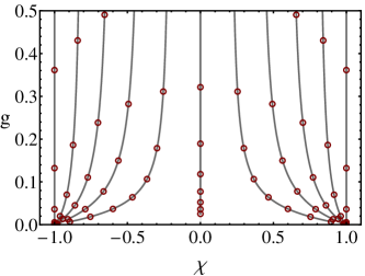
Figure 6: Flow of the conductance $g$ and the kink’s fugacity $\chi$ as a function of system size for class D system. Dots are for values, $L/\tilde{\xi}=1,2,4\dots,32$.

V.6 Boundary density of states

In the $L\to\infty$ critical points $\chi=-1/1$ the system does/does not support a Majorana state at its ends. In this limit, the bulk theory (by which we mean the bulk theory off criticality) becomes purely topological: the gradient term in (57) has scaled to zero, $\xi\to 0$. In the trivial phase of the $\chi=1$ – Anderson insulator, the story ends here. In the tAI phase $\chi=-1$ we are left with a term counting kink fugacities in terms of a phase action (58), at the fixed point, $\tilde{\chi}=-1$, the coefficient simplifies as $i\ln(\tilde{\chi})/\pi=-1$ and the topological action may be written as $S_{\mathrm{top}}[Q]=\mathrm{str}\left(\ln T(0)-\ln T(L)\right)$, i.e. as the sum of two boundary actions. These actions describe the boundary Green function at zero energy. Generalization to finite energies, $E$, is straightforward and leads to the left boundary action (analogously for the right)

$$S_{\mathrm{L}}[Q]=-\frac{\epsilon}{2}\,\mathrm{str}(Q\tau_{3})+\left(\frac{1-\chi}{2}\right)\mathrm{str}\ln(T),$$ (71)

where $\epsilon=\pi|E|/\Delta_{\xi}$ as in the AIII system and $\chi=\pm 1$ so that the form of the action is correct on both (AI and tAI) localized phases. The density of state deriving from this description has been computedIvanov (2002); Bagrets and Altland (2012) and reads as

$$\chi=1: \qquad\rho(\epsilon)=\frac{1}{\Delta_{\xi}}\left(1+\frac{\sin\epsilon}{\epsilon}\right),$$ (72)

$$\chi=-1: \qquad\rho(\epsilon)=\frac{1}{\Delta_{\xi}}\left(1-\frac{\sin\epsilon}{\epsilon}+\delta(\epsilon)\right).$$ (73)

The $\delta$-function in the second line is the topological Majorana state. Notice, however (see Ref. [Bagrets and Altland, 2012] for further discussion), that in either case, $\int_{-\epsilon_{0}}^{\epsilon_{0}}d\epsilon\,\rho(\epsilon)\stackrel{{\scriptstyle\epsilon_{0}\gg 1}}{{=}}2\epsilon_{0}+\frac{1}{2}$, i.e. the boundary accumulates an excess spectral weight of $1/2$, which in the non-topological case is the consequence of disorder generated quantum interference, and in the topological case due to the Majorana partially ‘screened’ by a negative interference contribution.

V.7 Class DIII

Model Hamiltonian — Similarly to class D, class DIII describes particle-hole symmetric, spin rotation non-invariant superconductors. The difference with class D is in the presence of time-reversal symmetry in class DIII. The Hamiltonian obeys a particle-hole symmetry, $H^{T}=-\sigma_{1}^{\mathrm{ph}}H\sigma_{1}^{\mathrm{ph}}$. Time reversal invariance requires $H^{T}=\sigma_{2}^{\mathrm{sp}}H\sigma_{2}^{\mathrm{sp}}$. These symmetries can be combined to obtain the chiral symmetry $P^{\dagger}HP=-H$ with $P=\sigma_{1}^{\rm ph}\otimes\sigma_{2}^{\rm sp}$. In the basis defined by this chiral structure, the Hamiltonian assumes the off-diagonal form

$$H^{\prime}=\left(\begin{array}[]{cc}&D\\ D^{\dagger}&\end{array}\right),\quad D^{T}=-D.$$ (74)

A generalization of the granular Hamiltonian (75) to the DIII symmetric situation reads

$$H=\sum_{ss^{\prime}}C_{-,s}^{\dagger}\left({\cal H}_{s}\delta_{ss^{\prime}}+iW\delta_{ss^{\prime}+1}\right)C_{+,s^{\prime}}+{\rm h.c.},$$ (75)

where $C_{\pm,s}^{\dagger}$ is a vector of creation operators on grain $s$ and the indices $(+/-)$ refer to the chiral structure. The $2N\times 2N$ matrix ${\cal H}=-{\cal H}^{T}$ is assumed to be random Gaussian distributed, while the $2N\times 2N$ hopping symmetric matrix, $W=W^{T}$, is translationally invariant and defines the non-random part of the Hamiltonian describing the inter-grain couplings.

Topological number — The definition of a topological number follows the lines of the construction in class D. We imagine the system closed to a ring and select one particular bond where $W^{\prime}=iW|+,1\rangle\langle-,0|$ is the hopping matrix associated to this bond. Representing the off-diagonal block of the Hamiltonian $H$ in the chiral basis (74) as $D=D^{\prime}+W^{\prime}$, the matrix $D_{\pi}=D^{\prime}-W^{\prime}$ represents a system with sign inverted hopping across the bond. The topological number can be now defined as ${\rm sgn}\left[{\rm Pf}(D_{\pi})/{\rm Pf}(D)\right]$. We show in Appendix D.3 that in the limit $L\to\infty$ this ratio of Pfaffians is a real number equal to $\pm 1$.

Field theory —The construction of a field theoretical partition sum parallels that of Section V.3 for the class D wire. Our starting point is a quadratic action $S[\bar{\Psi},\Psi]=\frac{1}{2}\bar{\Psi}(i0\tau_{3}-H)\Psi$, where $\Psi$ is an eight component field obeying the symmetry $\Psi=\sigma_{1}\otimes\tau\,\bar{\Psi}^{T}$, the matrix $\tau$ is defined as $\tau=i\tau_{2}\otimes{\cal P}^{\mathrm{b}}+\tau_{1}\otimes{\cal P}^{\mathrm{f}}$, and Pauli matrices $\sigma_{i}$ act in the ‘chiral’ space defined by Eq. (74). Resolving the chiral structure through $\Psi=(\Psi_{+},\Psi_{-})$, we have a continuous symmetry under transformations

$$\bar{\Psi}_{+}\to\bar{\Psi}_{+}T_{\mathrm{L}}, \quad\Psi_{+}\to T_{\mathrm{R}}^{-1}\Psi_{+}$$ (76)

$$\bar{\Psi}_{-}\to\bar{\Psi}_{-}T_{\mathrm{R}}, \quad\Psi_{-}\to T_{\mathrm{L}}^{-1}\Psi_{-}.$$ (77)

Here $T_{\mathrm{L},R}$ are $4\times 4$ matrices which act in the direct product of ${\rm bf}$ and ${\rm cc}$ spaces and belong to the group ${\rm SpO}(2|2)$ formed by all super-matrices of the type $T^{-1}=\tau T^{T}\tau^{-1}$. The full continuous symmetry group of the class $\mathrm{DIII}$ action thus is $G={\rm SpO}(2|2)\times{\rm SpO}(2|2)$, which as in the chiral class AIII will be broken to a single copy ${\rm SpO}(2|2)$ upon disorder averaging. A key feature of that manifold is that, as in class D, it is disconnected: the compact (fermionic) sector $\mathrm{O}(2)$ comprises fluctuations with determinant $\pm 1$, which cannot be continuously connected. Accordingly, the gauge symmetry group $G$ acting on the Goldstone mode manifold again contains a $\mathbb{Z}_{2}$ degree of freedom, generating kinks between the two disconnected components.

As before, we probe the system by insertion of topological gauge sources defined on one link $0\leftrightarrow 1$ only. To this end, let us generalize the operator connecting the corresponding sites as

$$\left(\begin{array}[]{cc}&W\\ W^{\dagger}&\end{array}\right)\to\left(\begin{array}[]{cc}&T_{L}(a)W\\ W^{\dagger}T_{R}^{-1}(a)&\end{array}\right).$$ (82)

Here, $T_{L}(a)$, where $a=(\phi,\sigma)$, $\phi=(-i\phi_{0},\phi_{1})^{T}$, and $\sigma=\pm$. While the general form of the transforming matrices is defined as

$$T_{L}(a) =e^{-\phi_{0}}\mathcal{P}^{\mathrm{b}}+e^{-i\phi_{1}}\tau_{1}^{(1-\sigma)/2}\mathcal{P}^{\mathrm{f}},$$ (83)

$$T_{R}(a) =e^{\phi_{0}}\mathcal{P}^{\mathrm{b}}+e^{i\phi_{1}}\mathcal{P}^{\mathrm{f}},$$ (84)

we will later apply the specific configurations $T_{L}(0,-)=\tilde{T}\equiv\mathcal{P}^{\mathrm{b}}+\mathcal{P}^{\mathrm{f}}\otimes\tau_{1}$, $T_{R}(0,-)=\mathds{1}$, and $T_{R}(\phi,+)=T_{L}^{-1}(\phi,+)=\mathrm{diag}(e^{\phi_{0}},e^{i\phi_{1}})^{\mathrm{bf}}$. Notice that the transformed operator lacks hermiticity, which indicates that the gauge transformations behind the insertion of the source are non-unitary chiral transformations. Indeed, a link modified as above can be generated by a transformation

$$T_{\mathrm{L/R,s}} =T_{\mathrm{L/R}}(a)\Theta(s)+\mathds{1}\Theta(-s).$$ (85)

The lattice-discontinuity across the $0\leftrightarrow 1$ link then generates the modified hopping operator. For a finite ring with periodic boundary conditions, the transformation above does not exist, implying that a single source link can be shifted through the system (by a boundary-consistent two-kink transformation), but not removed. The gauge transformation is described by two continuous variables $\phi$, and one $\mathbb{Z}_{2}$ variable $\sigma=\pm$, and we denote the corresponding partition function by $Z(a)\equiv Z^{(\sigma)}(\phi)$.

The sources above are constructed in such a way, that for $a=(0,-)$, $T_{\mathrm{L}}(0,-)=\mathcal{P}^{\mathrm{b}}+\mathcal{P}^{\mathrm{f}}\tau_{1}$, while $T_{R}=\mathds{1}$, i.e. in the fermionic sector the sourced link is replaced by $\tau_{1}$. Arguing as in the class D case, the corresponding partition function $Z^{(-)}(0)$ generates a product of Pfaffians with off-diagonal sector, $D$ and $D_{\pi}$, respectively (see previous section). In other words,

$$\chi=Z^{(-)}(0)=\left\langle\frac{\mathrm{Pf}(D_{\pi})}{\mathrm{Pf}(D)}\right\rangle.$$ (86)

By contrast, for $a=(\phi,+)$, $T_{L}=e^{i\phi}$. The link modified by the continuous parameters $\phi$ is to yield the conductance as in Eq. (13), i.e. with ${\cal F}(\phi_{0})=\partial_{\phi_{1}}Z^{(+)}(\phi)\bigl{|}_{\phi_{1}=-i\phi_{0}}$, we have $g=-i\partial_{\phi_{0}}{\cal F}(\phi_{0})\bigl{|}_{\phi_{0}=0}$.

Low-energy action — The field manifold $G/H={\rm SpO}(2|2)$ comprises a non-compact bosonic sector $\mathrm{Sp}(2)$, and the two-component $\mathrm{O}(2)$ in the fermionic sector. We parameterize the full manifold as

$$T^{(\pm)}=e^{\cal W}{\tilde{T}}^{(\pm)}e^{-{\cal W}},\qquad{\tilde{T}}^{(\pm)}=\left(\begin{array}[]{cc}{\tilde{T}}^{\mathrm{b}}&\\ &{\tilde{T}}^{\mathrm{f}(\pm)}\end{array}\right)^{\rm bf}.$$ (87)

The bosonic part is parametrized by one hyperbolic radial variable $y_{0}$ and two angles $\rho$ and $\alpha$

$${\tilde{T}}^{\mathrm{b}}=e^{i(b\tau_{+}+b^{*}\tau_{-})}e^{y_{0}\tau_{3}}e^{-i(b\tau_{+}+b^{*}\tau_{-})}$$ (88)

$$=\left(\begin{array}[]{cc}\cosh y_{0}+\cos 2\rho\sinh y_{0}&-ie^{i\alpha}\sin 2\rho\sinh y_{0}\\ ie^{-i\alpha}\sin 2\rho\sinh y_{0}&\cosh y_{0}-\cos 2\rho\sinh y_{0}\end{array}\right),$$ (91)

where $\rho=\sqrt{b^{*}b}$ and $e^{i\alpha}=\sqrt{b/b^{*}}$, and matrices $\tau_{i}$ act in charge conjugation space. The fermionic part is parameterized by a single compact radial variable $y_{1}$ and may be specified on the two parts of the group manifold

$${\tilde{T}}^{\mathrm{f}(+)}=e^{iy_{1}\tau_{3}}\,,\quad\quad{\tilde{T}}^{\mathrm{f}(-)}=\tau_{1}e^{iy_{1}\tau_{3}}\,.$$ (92)

Notice that only the $(+)$ manifold contains unit element and thus constitutes a subgroup. The boson-fermion rotations are parameterized by four Grassmann angular variables $\xi,\eta,\nu,\mu$ and restricted by the particle-hole symmetry ${\cal W}=-\tau{\cal W}^{T}\tau^{T}$,

$${\cal W}=\left(\begin{array}[]{cc}&{\cal B}\\ \tilde{\cal B}&\end{array}\right)^{\rm bf},\quad{\cal B}=\left(\begin{array}[]{cc}\xi&\nu\\ \mu&\eta\end{array}\right)^{\rm cc},\quad\tilde{\cal B}=\left(\begin{array}[]{cc}\eta&-\nu\\ \mu&-\xi\end{array}\right)^{\rm cc},$$ (93)

where $\tilde{\cal B}=-\tau_{1}{\cal B}^{T}i\tau_{2}$. A straightforward if somewhat lengthy calculation yields the Jacobians of the transformation to the above system of polar integration variables as

$$J^{(+)}={\sin 2\rho\over 2}\,\frac{\sinh^{2}y_{0}}{(\cosh y_{0}-\cos y_{1})^{2}}\,,\quad J^{(-)}={\sin 2\rho\over 2}\,.$$ (94)

Finally, the supersymmetric action of the array, written in terms of on-site group elements $T_{s}$ acquires the form (cf. Appendix D.3)

$$S[T]={1\over 4}\sum\limits_{s,k=1}^{L,4N}\mathrm{str}\ln\left[\openone+\frac{t_{k}^{2}}{4}\left(T_{s}^{-1}T_{s+1}+T_{s+1}^{-1}T_{s}-2\right)\right],$$ (95)

where $t_{k}$ are transmission matrix eigenvalues. This action is a counterpart of Eq. (55) for class $\mathrm{D}$. When subjected to a symbolic gradient expansion it takes the form $S[T]=-(\tilde{\xi}/8)\int\!dx\,\partial_{x}T^{-1}\partial_{x}T+\ln\tilde{\chi}\times n_{\mathrm{k}}$, where $\tilde{\xi}=g/2$, $g=\sum_{k=1}^{4N}t_{k}^{2}$ is the inter-dot conductance, and the second term represents the kink-action to be discussed momentarily. However, as with the class D system, a consistent treatment of kinks forces us to work with the granular action (95). Following the same recipe as in the class D case, we start by considering a configuration with one kink, where $T_{s}=\openone$, while $T_{s+1}={\tilde{T}}\equiv\mathcal{P}^{\mathrm{b}}+\mathcal{P}^{\mathrm{f}}\otimes\tau_{1}$. The corresponding contribution to the partition function acquires the form

$$e^{S(\mathds{1},\tilde{T})}=\prod\limits_{k=1}^{2N}r_{k}\!\!=\mathrm{Pf}\,(\hat{r}P)\equiv\tilde{\chi}\,,$$ (96)

where we took into account that all $4N$ eigenvalues $r_{k}=\pm(1-t_{k}^{2})^{1/2}$ of the transmission matrix $\hat{r}$ are Kramers degenerate and thus its Pfaffian may be defined as the product of $2N$ non-degenerate eigenvalues.

As in class D, we define a spinor partition function $Z_{s}=(Z^{(+)},Z^{(-)})_{s}^{T}$, where $Z^{(\pm)}$ describes the evolution of configurations starting at $T_{0}=\tau_{3}$ and ending at $T^{(\pm)}_{s}$ belonging to the same/opposite connectivity component. The evolution of the two-component $Z_{s}$ is described by the equation

$$Z^{(\sigma)}_{s+1}(T^{(\sigma)})=\sum_{\tilde{\sigma}=\pm}\int{\cal D}\tilde{T}^{(\tilde{\sigma})}\,\,e^{-S(T^{(\sigma)},\tilde{T}^{(\tilde{\sigma})})}\,Z^{(\tilde{\sigma})}_{s}(\tilde{T}^{(\tilde{\sigma})})\,,$$ (97)

We now again pass to the continuum limit, $Z_{s}\to Z(x)$ in which the diagonal blocks of the $2\times 2$ transfer operator become the standard Laplace-Beltrami operators $\sum_{\nu=\rho,y_{0},y_{1}}(J^{\pm})^{-1}\partial_{\nu}J^{\pm}\partial_{\nu}$ on the corresponding sector of the field manifold with Jacobians given by Eq. (94). The off-diagonal parts are somewhat more intricate. It turns out that the action $S(T^{(+)},\tilde{T}^{(-)})$ is independent of the compact radial variables $y_{1},\tilde{y}_{1}$ (while it still exhibits conventional Gaussian confinement $\sim g(y_{0}-\tilde{y}_{0})^{2}$ in the non-compact direction). As a result, the transfer matrix operator becomes a non-local integral operator in the compact $y_{1}$-direction. After Sutherland substitution $\Psi^{(\pm)}(y,x)=\Phi^{(\pm)}(y,x)/\sqrt{{\cal J}^{(\pm)}(y)}$ with ${\cal J}^{(\pm)}(y)=\partial_{\rho}J^{(\pm)}\bigl{|}_{\rho=0}$, it takes the form:

$$-\tilde{\xi}\,\partial_{x}\Phi=\left(\!\!\begin{array}[]{cc}\partial_{y_{0}}^{2}+\partial_{y_{1}}^{2}&-\displaystyle\tilde{\chi}\sqrt{g\over 2\pi}\,\partial_{y_{0}}\int\!d\tilde{y}_{1}\\ -\displaystyle\tilde{\chi}\sqrt{g\over 2\pi}\,\partial_{y_{0}}\int\!d\tilde{y}_{1}&\partial_{y_{0}}^{2}+\partial_{y_{1}}^{2}\end{array}\!\!\right)\Phi,$$ (98)

where we have denoted $\Phi=(\Phi^{(+)},\Phi^{(-)})^{T}$ and the length scale $\tilde{\xi}=g/2$ (in units of inter-dot spacing). This operator acts in the space of $2\pi$ periodic functions of $y_{1}$ (it is important that $\sqrt{{\cal J}^{(\pm)}(y)}$ are periodic), which may be written as $\Phi^{(\pm)}(y)=\sum_{l_{1}}\Phi^{(\pm)}_{l_{1}}(y_{0})e^{il_{1}y_{1}}$, with integer $l_{1}$. The $l_{1}\neq 0$ components are not affected by the kinks at all. The corresponding eigenvalues are $\epsilon(l_{0},l_{1}\neq 0)=l_{0}^{2}+l_{1}^{2}$, where $l_{0}\in\mathds{R}$ is a real quantum number from the non-compact direction $y_{0}$. On the other hand, the $\Phi^{(\pm)}_{0}(y_{0})$ spinor obeys the supersymmetric quantum mechanics (62) with $B^{(\dagger)}=-i\partial_{y_{0}}$, i.e. with zero super-potential $A=0$, and renormalized fugacity $\tilde{\chi}\to\tilde{\chi}\sqrt{2\pi g}$. The corresponding $l_{1}=0$ eigenvalue is $\epsilon(l_{0},0)=l_{0}^{2}+il_{0}\,\tilde{\chi}\sqrt{2\pi g}$. The eigenfunctions are the plane waves $\Phi_{l_{0},0}^{(\sigma)}(y_{0})=\frac{1}{\sqrt{2}}\,e^{il_{0}y_{0}}(1,\sigma)^{T}$, where $\sigma=\pm$, and again do not depend on the topological number $\tilde{\chi}$.

We now use the solution of the transfer matrix problem to extract observables. The measure is given by the overlap of the conjugated wave function with the initial conditions, $\mu(l)=-\langle\hat{\Psi}_{l}|(1,0)^{T}\rangle$. It leads to $\mu(l)=-2il_{0}/(l_{0}^{2}+l_{1}^{2})$, $l_{1}\neq 0$, and $\mu(l_{0},0)=\sqrt{2}i/l_{0}$ in case of $l_{1}=0$. It is clear that all components but $l_{1}=0$ decay exponentially on the scale given by the bare localization length $\tilde{\xi}\sim g$. Hereafter we thus focus exclusively on $l_{1}=0$ component, relevant for longer wires $L\gg\tilde{\xi}$. The corresponding partition sum spinor is given by

$$Z(\phi,L)=(1,0)^{T}+\int\frac{dl_{0}}{2\pi}\mu(l_{0},0)\Psi_{l_{0},0}(2\phi)e^{-\epsilon(l_{0},0)L/\tilde{\xi}},$$ (99)

where we put the radial coordinates to be $y=2\phi$, i.e. given by the boundary condition at $x=L$. Its $(-)$ component yields the renormalized fugacity as $\chi(L)=Z^{(-)}(0,L)$, Eq. (86). Referring for the details to Appendix C.3, we give below only the final result

$$\chi(L)=\mathrm{erf}\left(\tilde{\chi}\sqrt{\pi L}\right).$$ (100)

For $L\to\infty$ the renormalized fugacity exponentially approaches $\chi\to\mathrm{sign}(\tilde{\chi})=\pm 1$, indicating topologically trivial and non-trivial phases correspondingly. In turn, the conductance evaluated with the help of relation (13) takes the form

$$g(L)=4\,\sqrt{\frac{g}{\pi L}}\,e^{-\pi g\,\tilde{\chi}^{2}L/2\tilde{\xi}}.$$ (101)

We see that the average localization length, defined as

$$\xi=\frac{2\tilde{\xi}}{\pi g\,\tilde{\chi}^{2}}=\frac{1}{\pi\tilde{\chi}^{2}},$$ (102)

diverges towards the critical point $\tilde{\chi}=0$, resulting in the critical delocalized state with $g(L)\sim 1/\sqrt{L}$. At the same length scale $\xi$ the mean topological number $\chi(L)$, Eq. (100), approaches its quantized values $\pm 1$. The corresponding flow diagram on $(g(L),\chi(L))$ plane is qualitatively identical to the one in the class $\mathrm{D}$ shown in Fig. 6.

VI Scattering theory approach

In this section we discuss a relation of the SUSY partition function to the scattering matrix approach for mesoscopic wires. More precisely, we establish a formal equivalence of $Z(\phi,L)$ to the generating function of transmission eigenvalues for the wire of finite length $L$ connected to external leads. In classes $\mathrm{AIII}$ and $\mathrm{DIII}$, this enables us to get additional insights on localization/delocalization phenomena in topological 1d wires which go beyond the studies of conductance and average topological number. This section contains only the detailed statement of our results while its derivation is relegated to Appendix D.

We start with a summary of the relevant definitions made in previous sections. Our main object of study, the partition sum $Z(\phi)$, was defined as the disorder averaged ratio of the fermionic vs. bosonic determinants,

$$Z^{(+)}(\phi)=\left\langle\frac{Z_{F}(\phi_{1})}{Z_{B}(\phi_{0})}\right\rangle=\left\langle\frac{{\rm det}^{1/\nu}\left(i0^{+}\hat{\tau}-H(\phi_{1})\right)}{{\rm det}^{1/\nu}\left(i0^{+}\hat{\tau}-H(-i\phi_{0})\right)}\right\rangle.$$ (103)

The phase dependent Hamiltonian here is the result of non-local gauge transformation,

$$H_{ss^{\prime}}(\phi)=e^{-i\phi_{s}\hat{j}_{S}}H_{ss^{\prime}}e^{i\kappa\phi_{s^{\prime}}\hat{j}_{S}},\quad\kappa=\pm 1,$$ (104)

where the sign $\kappa=+1$ for class $\mathrm{D}$ and $\kappa=-1$ (i.e. the chiral gauge transform) is to be chosen for other classes ($\mathrm{AIII}$, $\,\,\mathrm{BDI}$ and $\mathrm{DIII}$). For $\mathds{Z}_{2}$-insulators $\hat{\tau}=\tau_{3}$ and $\nu=2$. In the case of $\mathds{Z}$-insulators, $\hat{\tau}=1$ and $\nu=1$. The appearance of $1/\nu$ power stems from the doubling procedure which was required for the proper construction of the path integral in the case of BdG classes $\mathrm{D}$ and $\mathrm{DIII}$. The generator $\hat{j}_{S}$ is related to the conserved current which choice depends on the symmetry class. The phase $\phi_{s}=0$ for sites with $s\leq 0$ and $\phi_{s}=\phi$ if $s\geq 1$. For the lattice model with the nearest neighbor hopping the phase dependent part of $H(\phi)$ is localized on a single link $0\leftrightarrow 1$. The generator $j_{S}$ of the symmetry current reads

$$\hat{j}_{S} = P,\qquad\quad\,\,\mbox{classes AIII, BDI};$$

$$\hat{j}_{S} = \tau_{1}^{\rm cc},\qquad\quad\!\!\mbox{class D};$$ (105)

$$\hat{j}_{S} = P\tau_{3}^{\rm cc},\qquad\mbox{class DIII}.$$

Here $P$ always denotes the parity operator, $\{P,H\}_{+}=0$, and $\tau$ matrices operate in charge-conjugation space. The ’minus’ component of the partition sum relevant for $\mathds{Z}_{2}$-insulators will be discussed later.

The partition sum (103) cast into the language of supersymmetric functional field integral was studied above. Our goal here is to relate $Z(\phi)$ to the scattering matrix of the disordered wire. More precisely, we assume that the system is now open to the external world rather than closed into the ring, meaning that the wire is connected to left/right leads. Then for any given realization of disorder potential the scattering ($\hat{S}$) and transfer ($\hat{M}$) matrices of dimension $2N^{\prime}\times 2N^{\prime}$ can be defined with $N^{\prime}$ being the number of scattering channels. For classes $\mathrm{AIII}$, $\mathrm{BDI}$ and $\mathrm{D}$ we have $N^{\prime}=2N$ where the factor $2$ is due to sub-lattice ($\mathrm{AIII}$) or particle-hole index (if classes $\mathrm{BDI}$ and $\mathrm{D}$ refer to spinless fermions). In the spinfull case and for class ${\mathrm{DIII}}$ one has $N^{\prime}=4N$ due to spin and p/h quantum numbers. With the use of DMPK theory both $\hat{S}$ and $\hat{M}$ can be reduced to the canonical formBrouwer et al. (1998, 2000b); Gruzberg et al. (2005). For the transfer matrix this representation takes the form

$$\hat{M}=\left(\begin{array}[]{cc}V&\\ &V^{\prime\dagger}\end{array}\right)\left(\begin{array}[]{cc}\cosh\lambda&\sinh\lambda\\ \sinh\lambda&\cosh\lambda\end{array}\right)\left(\begin{array}[]{cc}U^{\prime}&\\ &U^{\dagger}\end{array}\right),$$ (106)

where $\lambda={\rm diag}(\lambda_{1},\dots,\lambda_{N^{\prime}})$ is the set of so-called Lyapunov exponents and $U,V,U^{\prime},V^{\prime}\in\mathrm{U}(N^{\prime})$ are unitary matrices. Each exponent $\lambda_{k}$ defines the transmission coefficient $t_{k}^{2}=1/\cosh^{2}\lambda_{k}$ of the $k$-th transport channel.

Note that the flux conservation condition, $M^{\dagger}\sigma_{3}^{RL}M=\sigma_{3}^{RL}$, which stems from the hermicity of the underlying Hamitonian $\hat{H}$, is met by such form of $\hat{M}$. The presence of other non-unitary symmetries (time-reversal, particle-hole or parity) in the system puts additional constrains on the transfer matrix $\hat{M}$. They are specified by the basis dependent matrices $U_{T}$, $U_{C}$ and $P$. To proceed one should augment original spinors by the left/right grading, $\Psi=(\psi_{R},\psi_{L},\bar{\psi}_{L}^{T},\bar{\psi}_{R}^{T})$, to define the scattering states. This in turn requires the corresponding extension of the two symmetry matrices. Namely, ${\cal U}_{T}=\sigma^{RL}_{1}\otimes U_{T}$ becomes the proper matrix for time-reversal symmetry and ${\cal P}=\sigma^{RL}_{1}\otimes P$ should stand for the parity operator. Then time-reversal and particle-hole symmetries require ${\cal U}_{T}\hat{M}\,{\cal U}_{T}^{-1}=\hat{M}^{*}$ and $U_{C}\hat{M}\,U_{C}^{-1}=\hat{M}^{*}$, respectively, while the parity symmetry implies ${\cal P}\hat{M}\,{\cal P}=\hat{M}$, see e.g. Ref. [Brouwer et al., 2000b].

In application to the DMPK decomposition the chiral symmetry in $\mathds{Z}$-classes leads to relations $U^{\prime}=U^{\dagger}P$ and $V^{\prime}=V^{\dagger}P$. Besides that in chiral class $\mathrm{BDI}$ as well in class $\mathrm{D}$ it is advantageous to work in Majorana basis where the particle hole symmetry is the transposition ($H^{T}=-H$) with $U_{C}=\mathds{1}$. This reduces all rotation matrices to orthogonal ones, $\{U,V,U^{\prime},V^{\prime}\}\in\mathrm{SO}(N^{\prime})$. In class $\mathrm{DIII}$ the ancestor BdG Hamiltonian has the symmetry matrices $U_{C}=\sigma_{1}^{\rm ph}\otimes\mathds{1}^{\rm sp}$, $U_{T}=\mathds{1}^{\rm ph}\otimes\sigma_{2}^{\rm sp}$ and $P=U_{C}U_{T}^{-1}$. The choice of Majorana representation transforms them to $U_{C}=\mathds{1}$ and $P=U_{T}=\sigma_{3}^{\rm ph}\otimes\sigma_{2}^{\rm sp}$. In such basis channels’ transformations $V,U^{\prime}$ become orthogonal matrices, $\{V,U^{\prime}\}\in\mathrm{SO}(N^{\prime})$, defining the other two rotations according to $V^{\prime T}=P\,VP$ and $U^{T}=P\,U^{\prime}P$. It is worth mentioning here that the eigenvalues of any transfer matrix, $e^{\pm\lambda_{k}}$, always occur in inverse pairs. Moreover, in class $\mathrm{DIII}$ they are 2-fold degenerate pairs (Kramers’ degeneracy).

The symmetries of $\hat{M}$ listed above are strictly valid only at zero energy. Hence, when evaluating the determinant of the inverse Green’s function $G^{-1}_{\phi}=i\delta\hat{\tau}-H(\phi)$, we have to assume that a symmetry breaking term $i\delta\hat{\tau}$ is present only in the leads. This means that $\delta_{s}\equiv 0$ for cites with $0\leq s\leq L$ (inside the wire) and $\delta_{s}\to 0^{+}$ otherwise. With such regularization at hand ${\rm det}(G^{-1}_{\phi})$ is expressible via the set of Lyapunov exponents $\{\lambda_{k}\}$. Following Nazarov Nazarov (1994) we have accomplished this program using the method of quasiclassical Green’s functions with the ’twisted’ boundary conditions in the leads. The details of the calculations are presented in Appendix D, here we proceed further with the discussion of results.

For two $\mathds{Z}$-classes we have found

$$Z(\phi)=\left\langle\prod_{k=1}^{N^{\prime}}\frac{\cosh(\lambda_{k}+i\phi_{1})}{\cosh(\lambda_{k}+\phi_{0})}\right\rangle,$$ (107)

while for $\mathds{Z}_{2}$ topological wires the analogous ’plus’ partition sum reads

$$Z^{(+)}(\phi)=\left\langle\prod_{k=1}^{N^{\prime}}\left(\frac{\cosh(\lambda_{k}+i\phi_{1})\cosh(\lambda_{k}-i\phi_{1})}{\cosh(\lambda_{k}+\phi_{0})\cosh(\lambda_{k}-\phi_{0})}\right)^{1/2}\right\rangle.$$ (108)

In order to extract the physical observable we introduce the generating function (GF)

$${\cal F}(\phi_{0}) = \partial_{\phi_{1}}Z^{(+)}(\phi)\bigl{|}_{\phi_{1}=-i\phi_{0}}$$

$$= \nu^{-1}\langle{\rm tr}((-\partial_{\phi_{1}}H)G_{\phi_{1}})\rangle\bigl{|}_{\phi_{1}=-i\phi_{0}},$$

where the very last equality follows directly from Eq. (103). We see that GF is the zero energy expectation value of the symmetry current defined on a link $(0,1)$ with the help of the operator $\hat{\cal I}_{S}=-\partial_{\phi_{1}}H(\phi_{1})$. It is worth mentioning here that due to gauge invariance the position of the source $\phi_{0}$ can be shifted to any link. In this way one can define the current $\hat{\cal I}_{S}$ at each point of the wire. Thus obtained $\hat{\cal I}_{S}$ is the conserved Noether’s symmetry current and its average value is some analytical function of $\phi_{0}$ which is independent of the actual choice of the link.

Using now Eqs. (107, 108) we find

$${\cal F}(\phi_{0}) = i\sum_{k=1}^{N^{\prime}}\Bigl{\langle}\tanh(\phi_{0}+\lambda_{k})\Bigr{\rangle},\quad\mathds{Z}\,\mbox{-classes}.$$ (110)

$${\cal F}(\phi_{0}) = i\sum_{k=1}^{N^{\prime}}\left\langle\frac{\sinh 2\phi_{0}}{\cosh 2\lambda_{k}+\cosh 2\phi_{0}}\right\rangle,\quad\mathds{Z}_{2}\,\mbox{-classes}.$$

Following further the recipe (13) we first of all check that

$$g(L)=-i{\cal F}^{\prime}(0)=\sum_{k=1}^{N^{\prime}}\left\langle\frac{1}{\cosh^{2}\lambda_{k}}\right\rangle$$ (111)

is the (thermal) conductance at scale $L$, as expected. In application to the SUSY $\sigma$-model calculations such procedure works for three classes with the $P$-symmetry: $\mathrm{AIII}$, $\,\mathrm{BDI}$ and $\mathrm{DIII}$. In class $\mathrm{D}$ the low-energy field theory does not have the continuum phase $\phi_{1}$ in the fermionic sector and the evaluation of the generating function ${\cal F}$ introduced in Eq. (VI) becomes problematic. However, by setting $\phi_{1}=0$ one finds from Eq. (107) the series expansion

$$Z^{(+)}(\phi_{0},\phi_{1}=0)=1+\frac{1}{2}g(L)\phi_{0}^{2}+{\cal O}(\phi_{0}^{4}),$$ (112)

which proves that Eq. (51) is the conductance in this symmetry class.

As for the topological number $\chi$, we start from $\mathds{Z}$-insulators. According to the definition (13) we find

$$\chi(L)=\frac{1}{2}{\rm Im}\,{\cal F}(0)=\frac{1}{2}\sum_{k=1}^{N^{\prime}}\Bigl{\langle}\tanh\lambda_{k}\Bigr{\rangle}$$ (113)

In the trivial AI phase the number of positive and negative $\lambda$’s is equal and hence $\chi=0$. In the tAI phase all Lyapunov exponents satisfy $|\lambda_{n}|\gg 1$ and the topological number approaches an integer. In this phase the number of positive $\lambda$’s does not coincide with the number of negative ones. An integer $\chi$ changes by $\pm 1$ if any of $\lambda$’s changes sign when crossing the line of quantum phase transition. Exactly at the transition point the minimal Lyapunov exponent is zero, $\lambda_{\rm min}=0$, and hence $\chi$ takes a half-integer value.

The situation is more intricate for $\mathds{Z}_{2}$-wires where we have to know $Z^{-}$ partition sum to find the topological number $\chi$. In class $\mathrm{D}$ one can identify

$$Z^{(-)}=Z^{(+)}(\phi_{0}=0,\phi_{1}=\pi/2),$$ (114)

as the partition function of a kink’s configuration. The proof can be found in Appendix D.2. With the use of Eq. (107) this argument leads to:

$$\chi(L)=\Bigl{\langle}\prod_{k=1}^{N^{\prime}}\tanh\lambda_{k}\Bigr{\rangle}.$$ (115)

In the class $\mathrm{DIII}$ we have obtained the same result with the only difference that the product now is taken over $N^{\prime}/2=2N$ Lyapunov exponents, where each Kramers’ degenerate eigenvalue $\lambda_{k}$ is taken into account only once (cf. Appendix D.3).

We note that Eqs. (113) and (115) can be written in the basis independent form,

$$\chi(L) ={1\over 2}\langle{\rm tr}(\hat{r}P)\rangle,\quad\mbox{classes AIII, BDI};$$ (116)

$$\chi(L) =\langle{\rm det}(\hat{r})\rangle,\quad\quad\mbox{class D};$$ (117)

$$\chi(L) =\langle{\rm Pf}(\hat{r}P)\rangle,\quad\quad\!\!\mbox{class DIII},$$ (118)

where $\hat{r}$ is the reflection matrix of the wire. Deep in the localized phase, $L\gg\xi$ , the average topological number $\chi$ saturates to integer value. In this limit it coincides with the topological number ${\cal Q}$ introduced by Beenakker and co-workers Fulga et al. (2011). Relations (116-118) follow from the DMPK decomposition of the scattering matrix

$$\hat{S}=\left(\begin{array}[]{cc}U&\\ &V\end{array}\right)\left(\begin{array}[]{cc}\tanh{\lambda}&(\cosh{\lambda})^{-1}\\ (\cosh{\lambda})^{-1}&-\tanh{\lambda}\end{array}\right)\left(\begin{array}[]{cc}U^{\prime}&\\ &V^{\prime}\end{array}\right),\\$$

which gives for the reflection matrix $\hat{r}=U\tanh{\lambda}\,U^{\prime}$. Indeed, employing the symmetry constrains discussed previously we can state that $\hat{r}P=U\tanh{\lambda}\,U^{\dagger}$ in classes $\mathrm{AIII}$ and $\mathrm{BDI}$ and thereby Eq. (116) reduces to (113). In class $\mathrm{D}$ one has ${\rm detU}={\rm detU^{\prime}}=1$, by construction, so that Eq. (117) is in agreement with Eq. (115). Finally, in class $\mathrm{DIII}$ there is a basis where the parity operator should factorize into the product $P=\bigotimes_{k=1}^{2N}\Sigma_{y}$ where in the $k$-th block the corresponding Lyapunov exponent $\lambda_{k}$ is double degenerate. Hence $\hat{r}P=U\left(\bigotimes_{k=1}^{2N}\lambda_{k}\Sigma_{y}\right)U^{T}$ and the Pfaffian of this antisymmetric matrix simplifies to Eq. (115) where one substitutes $N^{\prime}\to N^{\prime}/2=2N$.

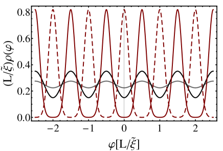
Figure 7: Average density of Lyapunov exponents $\rho(\phi)$ in the class $\mathrm{AIII}$ disordered wire in the case of $\tilde{\chi}=0$ shown for $L/\tilde{\xi}=1$ (weak localization — grey line), $L/\tilde{\xi}=4$ (black line) and $L/\tilde{\xi}=32$ (strong localization — solid read line) and in the case of $\tilde{\chi}=1/2$ for $L/\tilde{\xi}=32$ (dashed read line).

The generating function ${\cal F}(\phi_{0})$ can be used to recover the average density of Lyapunov exponentsLamacraft et al. (2004),

$$\rho(-\phi) = \sum_{k=1}^{N^{\prime}}\biggl{\langle}\delta(\phi+\lambda_{k})\biggr{\rangle}$$ (119)

$$= \frac{1}{2\pi}\Bigl{(}{\cal F}(\phi-i\pi/2)-{\cal F}(\phi+i\pi/2)\Bigr{)}.$$

From our SUSY calculations $\rho(\phi)$ is available analytically in two symmetry classes, $\mathrm{AIII}$ and $\mathrm{DIII}$. In the class $\mathrm{AIII}$ disordered wire, using the Poisson resummation formula, we have obtain from Eq. (25) the following result,

$$\rho(\phi;L) = \frac{\tilde{\xi}}{4L}+\sum_{n>0}(-)^{n}\frac{e^{-\pi^{2}n^{2}\tilde{\xi}/L}}{2\pi^{2}n}$$ (120)

$$\times \cos\bigl{(}2\pi n(\phi\tilde{\xi}/L-\tilde{\chi})\bigr{)}\sinh\frac{\pi^{2}n\tilde{\xi}}{L}.$$

The plot of this density, which shows the typical crystallization of Lyapunov exponents, is shown in Fig. 7. We note the periodic dependence on $\tilde{\chi}$. At $\tilde{\chi}=n+1/2$ the central peak is located at $\phi=0$ signaling the delocalized critical state. In the above result one should assume that the phase variable is limited to $\phi\in(-NL/\xi,NL/\xi)$, where $N$ is the number of channels.

In the class $\mathrm{DIII}$, using Eq. (99), one finds for the two minimal Lyapunov exponents the following average distribution

$$\rho(\phi;L) = 2\int\frac{dl_{0}}{\pi^{2}}\frac{\sinh\pi l_{0}}{l_{0}}\,\cos(2l_{0}\phi_{0})$$ (121)

$$\times \cos\!\left(\!\displaystyle\sqrt{2\pi g}\,\tilde{\chi}\,l_{0}\times\frac{L}{\tilde{\xi}}\right)\epsilon^{-l_{0}^{2}L/\tilde{\xi}},$$

which is normalized to $\int\rho(\phi;L)d\phi=2$. To quantify the crossover from the weak to strong localization in this distribution it is useful to introduce the renormalized bare fugacity $v=\tilde{\chi}\,\sqrt{2\pi g}$. The average localization length (102) then reads as $\xi=4\tilde{\xi}/v^{2}$, which is parametrically longer than $\tilde{\xi}$ in the limit $v\ll 1$. Figure 8 shows that at $L\gg\xi$ the ’crystallization’ of two minimal Lyapunov exponents occurs, with the most probable $\phi$’s being $\pm L/\xi_{*}$. Interestingly, the new length scale, $\xi_{*}=\tilde{\xi}/v$ (typical localization length), is parametrically different from $\xi$ (the average localization length) if $v\ll 1$. In the localized regime the length scale $\xi_{*}$ is defined by $\langle\ln g(L)\rangle\simeq-L/\xi_{*}$. The main contribution to the average of conductance, $\langle g(L)\rangle=\int d\phi\,\rho(\phi;L)$, however, come from the tails of the distribution $\rho(\phi;L)$ around $\phi=0$ resulting in the different length scale $\xi$ for the exponential decay $\langle g\rangle\sim e^{-L/\xi}$, such that in the close proximity to criticality one has $\xi\gg\xi_{*}$. The same conclusion has been reached in Ref. Gruzberg et al., 2005 on the basis of DMPK approach. Equation (121) also shows that for $v=0$ the maximum of the distribution is always located at $\phi=0$, corresponding to a perfectly transmitting channel, $t=1$. This is the origin of the delocalization in the absence of kinks. On the contrary, at $\tilde{\chi}\neq 0$ and large $L$ the perfect transmission is exponentially suppressed, signifying the localization.

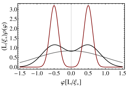
Figure 8: Average density of two minimal Lyapunov exponents $\rho(\phi)$ in the class $\mathrm{DIII}$ wire shown for the bare value of the renormalized fugacity $v=0.2$ (see the text) and $L/\tilde{\xi}=v,1,8$ (grey, black and read lines, resp.). In the limit $L\gg\xi\gg\tilde{\xi}$ (strong localization — red line) the minimal exponents ’crystallize’ around values $\pm L/2\xi_{*}$.

VII Comparison to $2d$

VII.1 The $\mathbb{Z}$-insulator classes: A,C, D

Historically, the first tI under consideration was the $2d$ integer quantum Hall effect. The importance of the static disorder in IQHE class A tI was emphasized right from the beginning (the reason being that the singular spectral of the clean bulk Landau level would not sit comfortably with observed data). The interplay of topological quantization and Anderson localization in the system found a powerful description in terms of Pruisken’s low energy field theoryPruisken (1984) already in 80th. In its subsequent supersymmetric formulationZirnbauer (1994) the Pruisken theory is described by the effective action,

$$S[Q]=\frac{1}{8}\int d^{2}x\,\left[-\tilde{g}\,\mathrm{str}(\partial_{\mu}Q\partial_{\mu}Q)+\tilde{\chi}\epsilon_{\mu\nu}\mathrm{str}(Q\partial_{\mu}Q\partial_{\nu}Q)\right],$$ (122)

where $\tilde{g}=\sigma^{0}_{xx}$ and $\tilde{\chi}=\sigma_{xy}^{0}$ are the bare ( Drude) values of longitudinal and Hall conductivities, respectively and $Q=T\tau_{3}T^{-1}$ takes values in the super-Riemannian space $\mathrm{U}(2|2)/\mathrm{U}(1|1)\times\mathrm{U}(1|1)$.

The Pruisken theory shows striking parallels to that of the $1d$ class $\mathbb{Z}$ – tI’s discussed above: (i) the theory assumes the form of a nonlinear $\sigma$-model containing a topological $\theta$-term (the second term in the action). (ii) Upon increasing length scales, the two parameters in the action renormalize according to Eq. (4). (iii) The renormalization of the topological parameter $\chi$ is driven by a proliferation of topological excitations in the system, which in $2d$ are instantons on the fermionic target space, $Q^{\mathrm{ff}}\in\mathrm{U}(2)/\mathrm{U}(1)\times\mathrm{U}(1)\simeq S^{2}$, the two-sphere. These excitations assume the role of the ‘phase’ windings’ in the $1d$ context. (iv) For generic values $\tilde{\chi}\notin\mathbb{Z}+\frac{1}{2}$, the flow towards an insulating configuration $g=\sigma_{xx}=0$ implies a restoration of the full symmetry under $G=\mathrm{U}(2|2)$ in the bulk. At the same time, the $\theta$-term at its fixed point coupling $\chi\in\mathbb{Z}$ becomes a boundary action of Wess- Zumino typeZirnbauer (1994), which describes the gapless propagation of boundary modes. (v) The observables $(g,\chi)$ can be extracted from the theory by coupling to topological sources, Pruisken’s background field methodPruisken (1984).

However, unlike the $1d$ $\mathbb{Z}$-systems, the critical physics of the IQHE system has not been quantitatively described beyond the weak coupling (large $g$) perturbative regime. The theory describing the QH fixed point, must be conformally invariant, a feature the Pruisken model lacks. One therefore expects a metamorphosis towards a conformally invariant fixed point theory along the flow on the $(g,\mathbb{Z}+1/2)$ critical surfaces. However, both the fixed point theory and the conversion mechanism were not identified so far.

The situation is different in the case of the class C topological insulator. This system, too, is described by a theory with Pruisken type action (122), the difference lying in the target space which now is $\mathrm{OSp}(2|2)/\mathrm{U}(1|1)$. All points (i)-(v) above remain valid as they stand, with the added feature that the critical point is under control: it has been shownGruzberg et al. (1999) that the class C quantum Hall transition belongs to the percolation universality class, which implies that its CFT is under control. By contrast, the class D system, another $2d$ class $\mathbb{Z}$ topological insulator, is not fully understood: as discussed above the class D field manifold contains two disjoint sectors. In $2d$, the ensuing $\mathbb{Z}_{2}$ leads to the emergence of Ising type criticality. It is believedBocquet et al. (2000), that this leads to the formation of a tri-critical point separating a topological and a non-topological insulator phase, and a (thermal) metal phase. For further discussion of this system, we refer to the literatureBocquet et al. (2000); Mildenberger et al. (2007)

VII.2 The $\mathbb{Z}_{2}$-insulator classes: AII, and DIII

Above we found that the $1d$ insulators of type $\mathbb{Z}$ and $\mathbb{Z}_{2}$, respectively were different in the nature of their topological structures: smooth instanton excitations vs. topological point defects. A similar dichotomy appears to be present in $2d$. While the class $\mathbb{Z}$ quantum Hall insulators of class A, C, D admit instantons as discussed in the previous subsection, a pioneering studyFu and Kane (2012) of Fu and Kane (KF) on the $\mathbb{Z}_{2}$ spin quantum Hall effect suggests that vortices with the point-like singularity in the middle are the relevant topological excitations of the system. The role of the $\theta$-term is taken by a contribution to the action $\ln\tilde{\chi}\times n_{\mathrm{v}}$, where $n_{\mathrm{v}}$ is the number of vortices. At criticality, the vortex fugacity vanishes $\tilde{\chi}\to 0$, and the resulting zero-vortex theory, $2d$ nonlinear $\sigma$-model belonging to the symplectic (AII) symmetry class exhibits delocalized behavior, expected of the critical system. The situation is a little more complicated due to the fact that a $2d$ system with vortices admits a Kosterlitz-Thouless transition. The analysis of KF indeed suggests that the KT transition points are positioned relative to the $\tilde{\chi}\to 0$ axis in such a way as to extend the metallic critical surface to a metallic phase (for further discussion of this point, we refer to the original reference [Fu and Kane, 2012]). Further, the KF analysis is based on a replica framework, in which the vortices are phase windings between select replicas. In view of the non-perturbative nature of these excitations, an adaption of the approach to the mathematically more rigorous framework of supersymmetry seems worthwhile. However, the topological structure of the corresponding supersymmetric field manifold, does not seem to support vortices, at lest not in the most obvious sense. Further work is required to better understand this point. In this context, it is worth mentioning the pivotal role of vortices played in metal-insulator transition governed by the topological Anderson localization in the two-dimensional disordered fermionic systems of chiral symmetry classes, as it was recently suggested by König et al. König et al. (2012) We finally note that the $2d$ DIII system — the time reversal invariant but spin rotation non- invariant $\mathbb{Z}_{2}$ topological superconductor – has not been addressed so far. However, the structure of its field manifold suggests that as in class AII topological point defects will be present.

We conclude that the list (i)-(iv) of $1d$–$2d$ analogies formulated above essentially generalizes to the $4$ $\mathbb{Z}_{2}$ systems. The main difference between the $\mathbb{Z}$ and the $\mathbb{Z}_{2}$ insulators is that the role of smooth instantons is taken by point defects, and that of field theoretical $\theta$-terms by fugacity terms. Without further discussion, we also note that the smooth/point-like dichotomy pertains to the realization of the topological sources, required to read out observables.

VIII Acknowledgments

Discussions with P. Brouwer and N. Read are gratefully acknowledged. AA and DB were supported by SFB/TR 12 of the Deutsche Forschungsgemeinschaft. AK was supported by NSF grant DMR1306734. AK also kindly acknowledges the hospitality of the International Faculty program at the University of Köln.

Appendix A Field theory of $\mathds{Z}$-insulators

We outline here the derivation of the field theory actions for classes $\mathrm{AIII}$ and $\mathrm{BDI}$ and discuss the self-consistent Born approximation (SCBA).

A.1 Class $\mathrm{AIII}$

The supersymmetric action of the $N$-channel disordered quantum wire corresponding to the microscopic model with the Hamiltonian (5) written in terms of the spinor $\psi=(\psi_{+},\psi_{-})$,

$$S = -\sum_{s}\left(\mu\,\bar{\psi}_{-,s}\psi_{+,s}+t\,\bar{\psi}_{-,s-1}\psi_{+,s}+{\rm h.c.}\right)+S_{\rm dis},$$

$$S_{\rm dis} = -\sum_{s,kk^{\prime}}\left(\bar{\psi}_{s+1,k}R^{kk^{\prime}}_{s+1,s}\psi_{s,k^{\prime}}+{\rm h.c.}\right),$$ (123)

where $\psi_{s}=\psi_{+,s/2}$ for $s$ even and $\psi_{s}=\psi_{-,(s-1)/2}$ for $s$ odd. Averaging $e^{-S_{\rm dis}}$ over the Gaussian fluctuations of disorder (6) one obtains the effective action containing the spatially local quartic term,

$$\tilde{S}_{\rm dis}=\frac{2w^{2}}{N}\sum_{s}{\rm str}\left(g^{++}_{s}g^{--}_{s}\right),$$ (124)

where we have introduced bilinears $g^{\alpha\beta}_{s}=\sum_{k}\psi_{\alpha,s,k}\otimes\bar{\psi}_{\beta,s,k}$. This term can be decoupled with the use of Hubbard-Stratonovich transformation by introducing two auxiliary $2\times 2$ matrix fields $Q^{\pm}_{s}=Q_{1,s}\pm iQ_{2,s}$ operating in the ${\rm bf}$-space. Integrating further over the $\psi$-fields, the partition sum assumes the form $Z=\int{\cal D}Q^{\pm}\,\exp(-S[Q])$, where

$$S[Q]=\frac{N}{2w^{2}}\sum_{s}{\rm str}(Q_{s}^{+}Q_{s}^{-})\,+\,{\rm str}\ln\!\left(\!\begin{array}[]{cc}i0-Q^{+}&-\hat{h}_{+}\\ -\hat{h}_{-}&i0-Q^{-}\end{array}\!\!\!\right)\!.$$ (125)

Here $\hat{h}_{\pm}$ are block matrices of the disorder independent Hamiltonian which in momentum space become $h_{\pm}(q)=\mu+te^{\pm iq}$.

Derivation of the sigma-model proceeds by subjecting the effective action $S[Q]$ to the saddle point analysis and identifying the soft Goldstone modes around the saddle point. Saddle point equations are known to be equivalent to the self-consistent Born approximation (SCBA) with the saddle point playing the role of the self-energy. In the present case they can be easily resolved by the ansatz $Q^{\pm}=-i\Sigma_{0}\sigma_{0}$, where $\Sigma_{0}\in\mathds{R}$. The solution of the SCBA equation,

$$-i\Sigma_{0} = w^{2}\,{\rm tr}\,\langle s|(i\Sigma_{0}-\hat{H}_{0})^{-1}|s\rangle,$$ (126)

is analyzed in the next subsection. Here $\hat{H}_{0}=\hat{h}_{+}\sigma_{+}+\hat{h}_{-}\sigma_{-}$, and the trace is taken with respect to the chiral space. Solving this equation, results in $\Sigma_{0}(\mu/t,w/t)$, which is a function of microscopic parameters in $H_{0}$ and the disorder strength $w$.

To identify the soft modes we substitute $iQ_{s}^{+}=\Sigma_{0}T_{s}$ and $iQ_{s}^{-}=T_{s}^{-1}\Sigma_{0}$ to find that

$$\!\!\!\!{\cal S}[T] = {\rm str}\ln\left(\begin{array}[]{cc}i\Sigma_{0}T&-\hat{h}_{+}\\ -\hat{h}_{-}&iT^{-1}\Sigma_{0}\end{array}\right)$$ (129)

$$= {\rm str}\ln\left(\begin{array}[]{cc}-i\Sigma_{0}&\hat{h}_{+}+T^{-1}[\hat{h}_{+},T]\\ \hat{h}_{-}&-i\Sigma_{0}\end{array}\right),$$ (132)

where the last equality results from the gauge transform of the ${\rm Sdet}$. Notice that for a uniform in space $T$-field the action ${\cal S}[T]$ is extremal and thus $\mathrm{GL}(1|1)$ is the Goldstone manifold of our problem and the field $T_{s}$, when slowly varying in space, is the soft-mode fluctuation. One also observes that ${\cal S}[T_{L}TT_{R}^{-1}]={\cal S}[T]$ which shows that the full symmetry group of the initial problem is $G=\mathrm{GL}(1|1)\otimes\mathrm{GL}(1|1)$, which is then broken to $G/\mathrm{GL}(1|1)$ after disorder averaging.

At the next step we expand the action ${\cal S}[T]$ in a gradient $\partial_{x}T(x)$ assuming this field is changing slowly on the lattice scale and thus passing to the continuum limit $s\to x$. To deal simultaneously with momentum and coordinate dependence of operators under the ${\rm str}$ we use the Moyal formula (’star’ product) $(A\star B)(x,q)=A\exp\{i(\overleftarrow{\partial_{x}}\overrightarrow{\partial_{q}}-\overleftarrow{\partial_{q}}\overrightarrow{\partial_{x}})/2\}B$ to evaluate the convolution of any two operators. Expanding the ’star’ product in gradients we get

$$T^{-1}[h_{+},T]\simeq-iv_{+}(q)\,T^{-1}\partial_{x}T+{\cal O}(\partial_{x}^{3}T)$$ (133)

with the complex ’velocities’ $v_{\pm}(q)=\partial_{q}h_{\pm}(q)\bigl{|}_{\Delta=t}=\pm it\,e^{\pm iq}$. The further expansion of ${\cal S}[T]$ up to second order in the field $\Phi_{x}=T^{-1}\partial_{x}T$ gives the low-energy field theoryAltland and Merkt (2001) with the action (18).

The microscopic value of the bare localization length $\tilde{\xi}$ is expressed in terms of velocity correlation function. Its exact value is of no importance for our consideration. In the limit of the weak disorder, $w\ll t\sim\mu$, one can estimate $\tilde{\xi}\sim Na(t/w)^{2}$ where $a$ is a lattice constant.

For the bare topological coupling constant one finds $\tilde{\chi}=i\langle G_{-+}^{R}(q)v_{+}(q)\rangle_{q}$ (with $G^{R}=(i\Sigma_{0}-\hat{H}_{0})^{-1}$ being the retarded SCBA Green’s function), which can be also written in the symmetrized form

$$\tilde{\chi}=\frac{i}{2}\langle{\rm tr}(G^{R}(q)P\partial_{q}H)\rangle_{q}.$$ (134)

It shows the relation of the bare topological topological number to the fictitious ’chiral’ persistent current, defined by the operator $\hat{j}_{c}(q)=P\hat{v}(q)$.

With the use of the $q$-representation the SCBA, Eq. (126), takes the form

$$1=2w^{2}\int_{-\pi}^{\pi}\frac{dq}{2\pi}\,\frac{1}{\Sigma_{0}^{2}+t^{2}+\mu^{2}+2\mu t\cos q}.$$ (135)

Performing the integration with the help of the residue theorem in a complex plane of a variable $z=e^{iq}$, the SCBA is reduced to $1=2w^{2}/{\cal D}$, where

$${\cal D}=\left(\Sigma_{0}^{2}+(t-\mu)^{2}\right)^{1/2}\left(\Sigma_{0}^{2}+(t+\mu)^{2}\right)^{1/2}.$$ (136)

From here $\Sigma_{0}$ can be explicitly found by resolving the quadratic equation. In the limit of small staggering and relatively weak disorder, i.e. at $|t-\mu|\ll w\ll t$, it reads $\Sigma_{0}=1/{2\tau}\simeq w^{2}/t$. Introducing the velocity $v=at$ one finds for the bare localization length $\tilde{\xi}\sim Nv\tau\sim Na(t/w)^{2}$ as stated in the main text.

Finally, substituting the SCBA Green’s function into Eq. (134), one obtains the bare topological number

$$\tilde{\chi}=\frac{N}{2}\left(1+(t/w)^{2}-\sqrt{1+t^{2}\mu^{2}/w^{4}}\right).$$ (137)

In the limit of small staggering it is simplified to

$$\tilde{\chi}=\frac{N}{2}\left(1+\frac{(t-\mu)t}{w^{2}}\right),\quad\quad|t-\mu|\ll w\ll t.$$ (138)

This bare topological number $\tilde{\chi}$ can be used to find the critical lines/surfaces of phase transition from the equation $\tilde{\chi}(\mu,t,w)=n+1/2$ with $n\in\mathds{Z}$. The corresponding lines are plotted in Fig. 4 for $N=3$.

A.2 Class BDI

Derivation of the sigma-model action in the class $\mathrm{BDI}$ system proceeds along the same lines as for the class $\mathrm{AIII}$. We start from the Hamiltonian (30) and transform it to the ’chiral’ basis where it has the block off-diagonal form, $\hat{H}=\hat{H}_{0}+\hat{V}\sigma_{1}$. Here $\hat{H}_{0}=\hat{h}_{+}\sigma_{+}+\hat{h}_{-}\sigma_{-}$ and the operators $\hat{h}_{\pm}$ in the $q$-space read $\hat{h}_{\pm}(q)=-(t+\cos q)\pm i\Delta\sin q$.

To construct the path-integral representation of $Z$ we consider the Gaussian action $S[\psi,\bar{\psi}]=\bar{\psi}(i0-\hat{H})\psi$ and following the doubling procedure detailed in sec. V.3 represent the former in the form, $S[\Psi]=\frac{1}{2}\bar{\Psi}(i0-\hat{H})\Psi$, where in class $\mathrm{BDI}$ the spinor $\bar{\Psi}=(\bar{\psi},\sigma^{\rm bf}_{3}\psi^{T})$, $\Psi=\tau\bar{\Psi}^{T}$ and the charge-conjugation matrix $\tau={\cal P}^{0}\otimes\tau_{1}+{\cal P}^{1}\otimes i\tau_{2}$. Subsequent disorder averaging over the Gaussian random matrices $\hat{V}_{s}$ at each site $s$ produces the quartic term

$$\tilde{S}_{\rm dis}=\frac{w^{2}}{2N}\sum_{s}{\rm str}\left(\sigma_{1}g_{s}\right)^{2},\quad g_{s}=\sum_{k}\Psi^{k}_{s}\otimes\bar{\Psi}^{k}_{s}.$$ (139)

This quadratic in $g_{s}$ form can be now decoupled by four $2\times 2$ super-matrix fields $P_{1,2}$ and $Q_{\pm}$ acting in the $\mathrm{cc}$-space, which is useful to combine into the single matrix $R$ with the structure in the chiral space,

$$R=\left(\begin{array}[]{cc}Q_{+}&P_{1}\\ P_{2}&Q_{-}\end{array}\right).$$ (140)

By doing so we obtain the following representation for the disorder averaged partition sum, $Z=\int{\cal D}(\Psi;R)\exp\left(-{\cal S}[\Psi,R]\right)$ with the action

$${\cal S}[\Psi,R]=\frac{N}{16w^{2}}{\rm str}(\sigma_{1}R)^{2}-\frac{i}{2}\bar{\Psi}(i0-\hat{H}_{0}-R)\Psi.$$ (141)

This action is gauge invariant under the $T$-rotations from the super-group $G=\mathrm{GL}(2|2)$ operating in the $\mathrm{cc}$ space. Namely, the transformation of the spinors

$$\Psi\rightarrow\left(\begin{array}[]{cc}\bar{T}^{-1}&\\ &T\end{array}\right)\Psi,\qquad\bar{\Psi}\rightarrow\bar{\Psi}\left(\begin{array}[]{cc}T^{-1}&\\ &\bar{T}\end{array}\right),$$ (142)

with the simultaneous transformation of matrix fields, $Q_{+}\to TQ_{+}\bar{T}$ and $Q_{-}\to\bar{T}^{-1}Q_{-}T^{-1}$ (we remind that the involution is defined as $\bar{T}=\tau T^{T}\tau^{T}$) leaves the action ${\cal S}$ invariant.

Next we perform the Gaussian integral over the $\Psi$-fields and reduce the partition function to the form $Z=\int{\cal D}R\,\exp(-S[R])$, where

$$S[R]=\frac{N}{16w^{2}}{\rm str}(\sigma_{1}R)^{2}+\frac{1}{2}{\rm str}\ln(i0-\hat{H}_{0}-R).$$ (143)

Extremizing this action, one obtains the saddle point $R=\hat{\Sigma}\equiv i\Sigma_{0}+\Sigma_{1}\sigma_{1}$, where two components of the self-energy $\Sigma_{0,1}\in\mathds{R}$ are to be found from the SCBA equation,

$$i\Sigma_{0} = w^{2}{\rm tr}\langle s|(i0-\hat{H}_{0}-\hat{\Sigma})^{-1}|s\rangle,$$ (144)

$$\Sigma_{1} = w^{2}{\rm tr}\langle s|(i0-\hat{H}_{0}-\hat{\Sigma})^{-1}\sigma_{1}|s\rangle.$$ (145)

We give its solution in the following subsection. The self-energy $\hat{\Sigma}$ is just one particular saddle of the action $S[R]$. Other possible extrema follow from the gauge invariance of the action under $T$-rotations. They generate the manifold of saddle points parametrized as

$$R=\left(\begin{array}[]{cc}i\Sigma_{0}\,T\bar{T}&\Sigma_{1}\,\mathds{1}^{cc}\otimes\mathds{1}^{\rm bf}\\ \Sigma_{1}\,\mathds{1}^{cc}\otimes\mathds{1}^{\rm bf}&i\Sigma_{0}\,(T\bar{T})^{-1}\end{array}\right),$$ (146)

The super-matrix $T$ is an element of the linear supergroup $G={\rm GL}(2|2)$. We see, however, that the subgroup of matrices $T^{\prime}$ satisfying the constraint $\bar{T}^{\prime}T^{\prime}=1$ does not affect the trivial saddle point. All matrices $T^{\prime}$ form the complex supergroup $H={\rm OSp}(2|2)$. Factoring out this subgroup we conclude that essential rotations are $T\in G/H={\rm GL}(2|2)/{\rm OSp}(2|2)$, which is the manifold of the soft (Goldstone) modes of the supersymmetric $\sigma$-model in the $\mathrm{BDI}$ symmetry class.

Similar to class $\mathrm{AIII}$ the final form of the $\sigma$-model (35) follows from the gradient expansion of the action ${\cal S}[T]$ with a smoothly varying matrix field $T(x)$ where

$${\cal S}[T]=$$ (147)

$$\frac{1}{2}{\rm str}\ln\left(\begin{array}[]{cc}-i\Sigma_{0}&\!\!\!\hat{h}_{+}+\Sigma_{1}+\Delta h_{+}\\ \hat{h}_{-}+\Sigma_{1}+\Delta h_{-}&\!\!\!-i\Sigma_{0}\end{array}\!\!\right).$$ (150)

Here we have defined $\Delta h_{+}=T^{-1}[\hat{h}_{+},T]$ and $\Delta h_{-}=\bar{T}[\hat{h}_{-},\bar{T}^{-1}]$, cf. Eq. (129). As a result of the gradient expansion one obtains the action (35) which is the functional of the field $Q=T\bar{T}$ with the same estimate for $\tilde{\xi}$ and the same formal result (134) for the bare topological number as in the case of class $\mathrm{AIII}$ system.

We now discuss the SCBA and derive the bare topological coupling constant $\tilde{\chi}$ for the model of disordered multi-channel p-wave superconducting wire. Transforming the self-consistent Green’s function to the momentum representation, using the explicit model form of $\hat{H}_{0}$ and introducing the notation $\tilde{\mu}=\mu-\Sigma_{1}$ one obtains two coupled SCBA equations (we limit ourselves to the special point $t=\Delta$ only)

$$\Sigma_{0} = 2w^{2}\int_{-\pi}^{\pi}\frac{dq}{2\pi}\frac{\Sigma_{0}}{\Sigma_{0}^{2}+\tilde{\mu}^{2}+t^{2}+2\tilde{\mu}t\cos q},$$

$$\Sigma_{1} = 2w^{2}\int_{-\pi}^{\pi}\frac{dq}{2\pi}\frac{\tilde{\mu}+t\cos q}{\Sigma_{0}^{2}+\tilde{\mu}^{2}+t^{2}+2\tilde{\mu}t\cos q}.$$ (151)

After $q$-integration, with the use of the function ${\cal D}$ defined above in Eq. (136) (where the substitution $\mu\to\tilde{\mu}$ is assumed), these equations are reduced to the coupled system of algebraic ones,

$$\Sigma_{0} = \frac{2w^{2}\Sigma_{0}}{{\cal D}},$$ (152)

$$\Sigma_{1} = \frac{w^{2}}{\mu-\Sigma_{1}}\left(1+\frac{(\mu-\Sigma_{1})^{2}-\Sigma_{0}^{2}-t^{2}}{{\cal D}}\right).$$

It follows from the 1-st equation that ${\cal D}=2w^{2}$, which then can be used to express $\Sigma_{0}$ via $\Sigma_{1}$ using the 2-nd equation. After these steps, employing the relation ${\cal D}=2w^{2}$ once again, one arrives to the quartic polynomial equation for $\Sigma_{1}$ which can be solved numerically. The self-energy $\hat{\Sigma}$ can be further used to find the SCBA topological number $\tilde{\chi}$. For the given model of p-wave disordered wire we have found from Eq. (134)

$$\tilde{\chi}(w,\mu)=\frac{N}{2}\left(1+\frac{t^{2}-\Sigma_{0}^{2}-(\mu-\Sigma_{1})^{2}}{2w^{2}}\right).$$ (153)

The above results can be simplified for the chemical potential in a close vicinity of the band edge, $|\mu-t|\ll t$, and at weak disorder, $w\ll t$. In this limit one can set ${\cal\tilde{D}}\simeq 1$. By defining the scattering rate as $1/\tau=Nw^{2}/t$ and the detuning from criticality $\bar{\mu}=\mu-t$, we have found

$$\Sigma_{0} = \frac{\sqrt{3}}{2}\left(\frac{1}{\tau}-\frac{\bar{\mu}}{3}\right)^{1/2}\left(\frac{1}{\tau}+\bar{\mu}\right)^{1/2},$$

$$\Sigma_{1} = -\frac{\bar{\mu}}{2}-\frac{1}{2\tau}$$ (154)

in the range $\bar{\mu}\in(-1/\tau,3/\tau)$ which is the interval of a non-vanishing mean DoS on the level of SCBA. Under the same assumptions the result (153) for the bare topological number is simplified to its approximate value (42) stated in the main text.

Appendix B Field theory of class $\mathrm{D}$

B.1 The Gaussian representation (47)

For the sake of completeness, we here briefly describe how the symmetries characterizing the Gaussian integral representation (47) are derived. The starting point is a ‘plain’ Gaussian super integral representation

$$Z=\left\langle\int d(\bar{\psi},\psi)\,e^{i\bar{\psi}(G^{+})^{-1}\psi}\right\rangle,$$ (155)

where $\psi=(\psi^{\mathrm{b}},\psi^{\mathrm{f}})$ is a vector comprising bosonic and Grassmann variables with components $\psi^{\alpha}=\{\psi^{\alpha}_{s,k}\}$. Notice that the symmetry $H^{T}=-H$ implies $(G^{+})^{T}=-G^{-}$. To see, how these symmetries entail an effective symmetry of the integration variables, we write

$$\bar{\psi}(G^{+})^{-1}\psi=\frac{1}{2}(\bar{\psi}(G^{+})^{-1}\psi+\bar{\psi}(G^{+})^{-1}\psi)=$$ (156)

$$=\frac{1}{2}\left(\bar{\psi}(G^{+})^{-1}\psi+(\bar{\psi}(G^{+})^{-1}\psi)^{T}\right)=$$ (157)

$$=\frac{1}{2}\left(\bar{\psi}(G^{+})^{-1}\psi-\psi^{T}\sigma_{3}^{\mathrm{bf}}(G^{-})^{-1}\bar{\psi}^{T}\right)\equiv$$ (158)

$$\equiv\bar{\Psi}\left(\begin{matrix}(G^{+})^{-1}&\crcr&(G^{-})^{-1}\end{matrix}\right)\Psi\equiv\bar{\Psi}G^{-1}\Psi,$$ (159)

where

$$\bar{\Psi}\equiv\frac{1}{\sqrt{2}}(\bar{\psi},-\psi^{T}\sigma_{3}^{\mathrm{bf}}),\qquad\frac{1}{\sqrt{2}}\Psi=\left(\begin{matrix}\psi\crcr\bar{\psi}^{T}\end{matrix}\right).$$ (160)

In the second line, we used that the number $\bar{\psi}(G^{+})^{-1}\psi$ is equal to its transposed, and in the third that the transposition of a Grassmann bilinear form $\bar{\psi}^{1}(G^{+})^{-1}\psi^{1}=-\psi^{1T}(G^{+})^{-1T}\bar{\psi}^{1T}$ introduces an extra minus sign. The two component structure introduced in Eq. (160) defines the space of $\tau$-matrices. From the structure of $\Psi$ and $\bar{\Psi}$, one reads out the symmetry (48), and that $G^{-1}=i0\tau_{3}-H$.

B.2 Jacobians

Here we calculate Jacobians on the two parts of the manifold. To this end we write $Q^{(\pm)}=e^{\cal W}{\tilde{Q}}^{(\pm)}e^{-{\cal W}}$, Eq. (52), and differentiate over parameters. In doing it we choose to stay near zero Grassmanns for simplicity, since Jacobians are expected to be Grassmann-independent $dQ^{(\pm)}=[d{\cal W},{\tilde{Q}}^{(\pm)}]+d{\tilde{Q}}^{(\pm)}$ and $dQ^{(\pm)-1}=[d{\cal W},{\tilde{Q}}^{(\pm)-1}]+d{\tilde{Q}}^{(\pm)-1}$. The metric is given by

$$dg = -{1\over 8}{\rm str}\left(dQdQ^{-1}\right)$$

$$= -{1\over 8}{\rm str}\left([d{\cal W},{\tilde{Q}}][d{\cal W},{\tilde{Q}}^{-1}]\right)-{1\over 8}{\rm str}\left(d{\tilde{Q}}d{\tilde{Q}}^{-1}\right)$$

Substituting the parametrization (52-54), one finds for the “plus” manifold

$$dg^{(+)} = dy^{2}+\sinh^{2}2y\,\,d\alpha^{2}+2\eta\xi\sinh^{2}y$$ (162)

and therefore

$$J^{(+)}=\sqrt{\mathrm{Sdet}g^{(+)}}=\,\frac{\sinh 2y}{\sinh^{2}y}=2\coth y$$ (163)

In a similar way, for “minus” part of the manifold one finds

$$dg^{(-)}=dy^{2}+\sinh^{2}2y\,\,d\alpha^{2}-2\eta\xi\cosh^{2}y.$$ (164)

The minus sign in the last term implies the opposite sign of the Grassmann measure.

$$J^{(-)}=\sqrt{\mathrm{Sdet}g^{(-)}}=\,\frac{\sinh 2y}{\cosh^{2}y}=2\tanh y$$ (165)

B.3 Transfer Matrix

Our goal is to calculate transfer matrix element between two neighboring grains $e^{-S(Q^{(\alpha)},\tilde{Q}^{(\beta)})}$, where $\alpha,\beta=\pm$ denote two parts of the manifold, and

$$S(Q,\tilde{Q})=\frac{1}{4}\sum_{k=1}^{2N}{\rm str}\ln\left[1+\frac{t_{k}^{2}}{4}(\{Q,\tilde{Q}\}_{+}-2)\right].$$ (166)

This operator acts on the two-component spinor wave function $\Psi(\tilde{Q})=\Psi^{(\beta)}(\tilde{y})$, which is assumed to depend only on the radial variable $\tilde{y}$, but not on the bosonic angle $\tilde{\alpha}$ or Grassmann variables $\tilde{\eta},\tilde{\xi}$. The entire angle/Grassmann dependence is thus restricted to the transfer matrix element and may be integrated out explicitly. We thus define the radial part of the transfer operator as

$${\cal R}^{(\alpha\beta)}(y;\tilde{y})=\int\frac{d\tilde{\alpha}}{2\pi}\,d\tilde{\eta}\,d\tilde{\xi}\,(\beta)J^{(\beta)}(\tilde{y})\,e^{-S(Q^{(\alpha)},\tilde{Q}^{(\beta)})},$$ (167)

where factor $(\beta)$ reflects opposite sign of the Grassmann measure on the $(-)$ manifold. As a result of the angular-rotational invariance the element $Q^{(\alpha)}=Q^{(\alpha)}(y)$ may be assumed to be pure radial as well (i.e. taken e.g. at zero angles). We now substitute such $Q^{(\alpha)}(y)$ and $\tilde{Q}^{(\beta)}(\tilde{y},\tilde{\alpha},\tilde{\eta},\tilde{\xi})$ into the action (166) and find:

$$S=g\big{[}S_{0}^{(\alpha\beta)}(y;\tilde{y},\tilde{\alpha})+\tilde{\eta}\,\tilde{\xi}\,F^{(\alpha\beta)}(y;\tilde{y},\tilde{\alpha})\big{]},$$ (168)

where $S_{0}^{(\alpha\beta)}$ is the part of the action which does not contain Grassmanians and $g=\sum_{k}t_{k}^{2}\gg 1$. We then expand $e^{g\tilde{\eta}\,\tilde{\xi}F^{(\alpha\beta)}}$ to the first order, integrate over Grassmann variables and obtain

$${\cal R}^{(\alpha\beta)}(y;\tilde{y})=g\int\frac{d\tilde{\alpha}}{2\pi}\,(\beta)J^{(\beta)}(\tilde{y})\,F^{(\alpha\beta)}\,e^{-gS_{0}^{(\alpha\beta)}}.$$ (169)

The straightforward, though lengthy, calculation yields:

$$S_{0}^{(\pm\pm)} = \frac{1}{4}\cosh 2y\cosh 2\tilde{y}$$

$$- \frac{1}{4}\cos 2\tilde{\alpha}\sinh 2y\sinh 2\tilde{y}-\frac{1}{4}$$

$$\simeq \frac{1}{2}(\tilde{y}-y)^{2}+\frac{\tilde{\alpha}^{2}}{2}\sinh 2y\sinh 2\tilde{y},$$

and

$$S_{0}^{(\pm\mp)}=-\ln\tilde{\chi}+S_{0}^{(\pm\pm)},$$ (171)

where we have defined the kink fugacity,

$$\tilde{\chi}=\pm\prod_{k=1}^{2N}(1-t_{k}^{2})^{1/2}$$ (172)

In the limit $g\gg 1$ the angular integration is dominated by the saddle point at $\tilde{\alpha}=0$, while the radial one by $\tilde{y}=y$. We thus restrict ourselves to the vicinity of these saddle points, where

$$F^{(++)}(y;\tilde{y},0) = \sinh y\sinh\tilde{y}\cosh(\tilde{y}-y),$$

$$F^{(--)}(y;\tilde{y},0) = -\cosh y\cosh\tilde{y}\cosh(\tilde{y}-y),$$

$$F^{(+-)}(y;\tilde{y},\tilde{\alpha}) = \cosh\tilde{y}\sinh y\sinh(\tilde{y}-y)$$

$$- {\tilde{\alpha}^{2}\over 2}\sinh 2y\sinh 2\tilde{y}+{\cal O}(\tilde{\alpha}^{3}),$$

$$F^{(-+)}(y;\tilde{y},\tilde{\alpha}) = -\cosh y\sinh\tilde{y}\sinh(\tilde{y}-y)$$

$$- {\tilde{\alpha}^{2}\over 2}\sinh 2y\sinh 2\tilde{y}+{\cal O}(\tilde{\alpha}^{3}),$$

and in the off-diagonal terms we kept a term $\propto\tilde{\alpha}^{2}$.

We first evaluate $\tilde{\alpha}$ integral in the Gaussian approximation near $\tilde{\alpha}=0$:

$${\cal R}^{(++)}=\sqrt{\frac{g}{2\pi}}\,\,\sqrt{\frac{\coth\tilde{y}}{\coth y}}\cosh(\tilde{y}-y)e^{-g(\tilde{y}-y)^{2}/2}.$$

Integrating over $\tilde{y}$ in the saddle point approximation yields unity in agreement with SUSY normalization. Similar calculation works for ${\cal R}^{(--)}$. Going beyond this approximation, requires expanding pre-exponential factors, including wave factions, to second order in $\delta y=\tilde{y}-y$. This leads to standard Laplace-Beltrami operators $\frac{1}{2}(J^{(\pm)})^{-1}\partial_{y}(J^{(\pm)}\partial_{y})$.

We turn now to the off-diagonal parts. The off-diagonal fermionic $F$-factors, being calculated at the saddle point $\tilde{\alpha}=0$ and $\tilde{y}=y$ yield zero $F^{(\pm\mp)}(y;y,0)=0$. This is again a manifestation of the SUSY normalization. One has to go thus beyond the saddle point approximation, keeping the deviations from the saddle point. This way one finds for the off-diagonal components of the transfer operator

$${\cal R}^{(+-)}(y;\tilde{y}) \simeq -\tilde{\chi}\sqrt{\frac{g}{2\pi}}\,e^{-g(\delta y)^{2}/2}\Bigl{[}-{1\over 2g}\frac{1}{\cosh^{2}y}$$ (173)

$$+ \tanh y\,\delta y+\frac{(\delta y)^{2}}{2\cosh^{2}y}\Bigr{]},$$

$${\cal R}^{(-+)}(y;\tilde{y}) \simeq -\tilde{\chi}{\sqrt{\frac{g}{2\pi}}}\,e^{-g(\delta y)^{2}/2}\Bigl{[}{1\over 2g}\frac{1}{\sinh^{2}y}$$ (174)

$$+ \coth y\,\delta y-\frac{(\delta y)^{2}}{2\sinh^{2}y}\Bigr{]},$$

where we kept the expansion up to the second order in $\delta y=\tilde{y}-y$. We now consider how these operators act on the radial wave function

$$\Psi^{(\pm)}(\tilde{y})=\Psi^{(\pm)}(y)+\partial_{y}\Psi^{(\pm)}(y)\,\delta y+{\cal O}(\delta y^{2}).$$ (175)

In view of the relation

$$\int d\tilde{y}e^{-g(\delta y)^{2}/2}(\delta y)^{2}/\int d\tilde{y}e^{-g(\delta y)^{2}/2}=g^{-1},$$

the zeroth order term $\Psi^{(\pm)}(y)$ does not contribute. This is again a manifestation of SUSY normalization, which manifests itself as a cancellation of subleading terms originating from $\tilde{\alpha}^{2}$ and $(\delta y)^{2}$. The remaining terms come solely from $\partial_{y}\Psi^{(\pm)}(y)\,\delta y$ and term linear in $\delta y$ in Eqs. (173) and (174). Upon Gaussian integration over $\delta y$, this yields

$${\cal R}^{(+-)}\Psi^{(-)}=-\frac{\tilde{\chi}}{g}\,\tanh y\,\,\partial_{y}\Psi^{(-)}=-\frac{\tilde{\chi}}{g}\,\sqrt{\frac{J^{(-)}}{J^{(+)}}}\,\partial_{y}\Psi^{(-)},$$

$${\cal R}^{(-+)}\Psi^{(+)}=-\frac{\tilde{\chi}}{g}\,\coth y\,\,\partial_{y}\Psi^{(+)}=-\frac{\tilde{\chi}}{g}\,\sqrt{\frac{J^{(+)}}{J^{(-)}}}\,\partial_{y}\Psi^{(+)}.$$

Introducing continious space derivative as $\partial_{x}\Psi=\Psi_{s+1}-\Psi_{s}=[\hat{\cal R}-1]\Psi$, one may write in the matrix form:

$$-\tilde{\xi}\partial_{x}\hat{\Psi}=\left(\begin{array}[]{cc}{1\over 2J^{(+)}}\partial_{y}J^{(+)}\partial_{y}&-\tilde{\chi}\sqrt{\frac{J^{(-)}}{J^{(+)}}}\,\partial_{y}\\ -\tilde{\chi}\sqrt{\frac{J^{(+)}}{J^{(-)}}}\,\partial_{y}&{1\over 2J^{(-)}}\partial_{y}J^{(-)}\partial_{y}\end{array}\right)\!\left(\begin{array}[]{c}\Psi^{(+)}\\ \Psi^{(-)}\end{array}\right).$$ (176)

Notice that $\hat{\Psi}={\rm const}$ manifestly nullifies the right hand side in accord with the SUSY normalization.

After the Sutherland substitution: $\Phi^{(\pm)}=\sqrt{J^{(\pm)}}\Psi^{(\pm)}$ one finds:

$$\tilde{\xi}\partial_{x}\hat{\Phi}=\left(\begin{array}[]{cc}-\frac{1}{2}\partial_{y}^{2}+V^{(+)}(y)&\tilde{\chi}\left[\partial_{y}-A^{(-)}(y)\right]\\ \tilde{\chi}\left[\partial_{y}-A^{(+)}(y)\right]&-\frac{1}{2}\partial_{y}^{2}+V^{(-)}(y)\end{array}\right)\hat{\Phi},$$ (177)

where $A^{(\pm)}(y)=\partial_{y}\sqrt{J^{(\pm)}}/\sqrt{J^{(\pm)}}=\mp 2\lambda/\sinh 2y$ and

$$V^{(\pm)}(y)=\frac{\partial^{2}_{y}\sqrt{J^{(\pm)}}}{2\sqrt{J^{(\pm)}}}=-\frac{\lambda(\lambda\mp 1)}{2\cosh^{2}y}+\frac{\lambda(\lambda\pm 1)}{2\sinh^{2}y}$$ (178)

are modified Pöschel-Teller potentialsBarut et al. (1987) with $\lambda=1/2$. Equation (177) may be rewritten in the manifestly supersymmetric form (62), (63).

Looking for the “stationary” solutions in the form $\hat{\Phi}(y,x)=\hat{\Phi}_{l}(y)e^{-\epsilon(l)x/\tilde{\xi}}$, one finds for the spectrum of the transfer matrix operator $\epsilon(l)=l^{2}/2+i\,\tilde{\chi}\,l$, where $l$ labels the eigenfunctions according to their asymptotic behavior $\hat{\Phi}_{l}\sim e^{ily}$. The supersymmetric form (62), (63) of the transfer matrix operator insures that the eigenfunctions do not depend on the fugacity $\tilde{\chi}$ and are those of the modified Pöschel-Teller potentials (178). Their explicit form is given byBarut et al. (1987)

$$\Phi^{(+)}_{l} = \frac{1}{\sqrt{N^{+}_{l}}}\,_{2}F_{1}\Bigl{(}1\!-\!\frac{il}{2},1\!-\!\frac{il}{2},2;1\!-\!z\Bigr{)}(1-z)^{3/4}z^{-il/2}$$

$$\Phi^{(-)}_{l} = \frac{-i}{\sqrt{N^{-}_{l}}}\,_{2}F_{1}\Bigl{(}1-\frac{il}{2},-\frac{il}{2},1;1\!-\!z\Bigr{)}(1-z)^{1/4}z^{-il/2},$$

where $z=1/\cosh^{2}y$ and $N^{\pm}_{l}$ are $l$-dependent normalization constants. To find $N^{+}_{l}$ one should explore the asymptotic of $\Phi^{(+)}$ at $y\to+\infty$, which corresponds to $z\to+0$, where

$${}_{2}F_{1}\Bigl{(}1-\frac{il}{2},1-\frac{il}{2},2;1-z\Bigr{)}\sim\frac{\Gamma(il)}{\Gamma^{2}(1+il/2)}+\frac{\Gamma(-il)z^{il}}{\Gamma^{2}(1-il/2)},$$

and since $z\sim 4e^{-2y}$ at $y\to+\infty$ one finds

$$\Phi^{(+)}_{l}(y)\sim\frac{1}{\sqrt{N^{+}_{l}}}\left\{\frac{\Gamma(il)e^{il(y-\ln 2)}}{\Gamma^{2}(1+il/2)}+{\rm c.c.}\right\}.$$ (179)

Requiring the asymptotic condition

$$\Phi^{(\pm)}_{l}(y)\sim\cos(ly+\delta^{\pm}_{l}),$$ (180)

at infinity with $\delta^{\pm}_{l}$ being some phase shifts, one finds

$$N^{+}_{l} = \left|\frac{2\,\Gamma(il)}{\Gamma^{2}(1+il/2)}\right|^{2}=\frac{8\tanh\left(\frac{\pi l}{2}\right)}{\pi l^{3}},$$

$$N^{-}_{l} = \left|\frac{2\,\Gamma(il)}{\Gamma\left(\frac{il}{2}+1\right)\Gamma\left(\frac{il}{2}\right)}\right|^{2}=\frac{2\tanh\left(\frac{\pi l}{2}\right)}{\pi l}.$$

where $N^{-}_{l}$ is found in the similar way. We note that the phase shifts satisfy $\delta^{-}_{l}=\delta^{+}_{l}+\pi/2$ and hence

$$\Phi^{(-)}_{l}(y)\sim-i\cos(ly+\delta^{-}_{l})\sim i\sin(ly+\delta^{+}_{l}),\quad y\to+\infty.$$

The latter asymptote is consistent with the mutual relation between two solutions $\Phi_{l}^{+}$ and $\Phi_{l}^{-}$ of Pöschel-Teller potential, namely:

$$(B\Phi^{(+)}_{l})/(-il)\sim\partial_{y}\Phi^{(+)}_{l}/(il)\sim i\sin(ly+\delta_{l}^{+})\sim\Phi^{(-)}_{l},$$

as it should be.

B.4 Observables

We start by evaluating the measure,

$$\mu(l)=-\langle(1,0)|\Psi_{l}\rangle=\int_{0}^{+\infty}\!\!dy\,\,\sqrt{J^{(+)}(y)}\,\Phi_{l}^{(+)}(y)$$ (181)

Using the explicit form of $\Phi^{(+)}(y)$ and changing the variable of integration to $u=\tanh^{2}y$, one obtains

$$\mu(l)\! = \!\frac{-1}{\sqrt{2N^{+}_{l}}}\int_{0}^{1}\!\!du\,(1-u)^{-1-il/2}{{}_{2}F_{1}}\!\Bigl{(}\!1\!-\!\frac{il}{2},1\!-\!\frac{il}{2},2;u\!\Bigr{)}$$

$$= \frac{-1}{\sqrt{2N^{+}_{l}}}\times\frac{4}{l^{2}}=-\sqrt{\frac{\pi}{l\tanh\frac{\pi l}{2}}}.$$

The wave function with the proper initial, i.e. $x=0$, conditions is given by

$$\Psi(y,x)=\left(\!\begin{array}[]{c}1\\ 0\end{array}\!\right)+\int\!\!\frac{dl}{2\pi}\mu(l)\left(\!\begin{array}[]{c}\Phi^{(+)}_{l}(y)/\sqrt{J^{(+)}}\\ \Phi^{(-)}_{l}(y)/\sqrt{J^{(-)}}\end{array}\!\right)\,e^{-\epsilon(l)x/\tilde{\xi}}$$

Let us first focus on the $(-)$ component and evaluate the renormalized topological number $\chi(L)=\Psi^{(-)}(0,L)$. Evaluating the limiting value

$$\lim_{y\to 0}\Phi_{l}^{(-)}(y)/\sqrt{J^{(-)}(y)}=-{i}/{\sqrt{2N_{l}^{-}}},$$

we obtain

$$\chi(L)=\int\limits_{0}^{+\infty}\!\!dl\,\coth\left(\frac{\pi l}{2}\right)\sin\left(\frac{\tilde{\chi}lL}{\tilde{\xi}}\right)e^{-l^{2}L/(2\tilde{\xi})}.$$ (183)

In the limit of long system, $L\gg\xi=2\tilde{\xi}\,\tilde{\chi}^{-2}$, one finds

$$\chi(L)\simeq\mathrm{sign}\,\tilde{\chi}\left(1-\sqrt{\frac{\xi}{\pi L}}\,e^{-{L/\xi}}\right).$$ (184)

Therefore the topological number approaches exponentially the quantized limiting value $\pm 1$, which indicates topologically trivial/non-trivial phase.

To evaluate the renormalized conductance we use $g(L)=\partial_{y}^{2}\Psi^{(+)}(y,L)\bigl{|}_{y=0}$ to obtain

$$g(L) = \frac{1}{4}\int\limits_{0}^{+\infty}dl\,l\coth\left(\frac{\pi l}{2}\right)\cos\left(\frac{\tilde{\chi}lL}{\tilde{\xi}}\right)e^{-l^{2}L/(2\tilde{\xi})}$$ (185)

$$\propto \frac{1}{\sqrt{L}}\,e^{-L/\xi},$$

in the limit $L\gg\xi$. Therefore, unless $\tilde{\chi}=0$, the conductance is exponentially small, indicating the Anderson insulator nature of the class $\mathrm{D}$ quasi-1d system.

Appendix C Field theory of class $\mathrm{DIII}$

C.1 Jacobians

We start by evaluating Jacobians on two disconnected parts of the group manifold. Following Eq. (87) we parametrize the group element as $T^{(\pm)}=e^{{\cal W}}{\tilde{T}}^{(\pm)}e^{-{\cal W}}$ and further find the metric on the group in the chosen coordinates. As in class $\mathrm{D}$ we choose to stay near zero Grassmans, since in what follows we will need only the Grassmann independent part of Jacobians. Using $dT^{(\pm)}=[d{\cal W},{\tilde{T}}^{(\pm)}]+d{\tilde{T}}^{(\pm)}$ and $dT^{(\pm)-1}=[d{\cal W},{\tilde{T}}^{(\pm)-1}]+d{\tilde{T}}^{(\pm)-1}$, the metric is given by

$$dg = -{1\over 2}{\rm str}\left(dTdT^{-1}\right)$$

$$= -{1\over 2}{\rm str}\left([d{\cal W},{\tilde{T}}][d{\cal W},{\tilde{T}}^{-1}]\right)-{1\over 2}{\rm str}\left(d{\tilde{T}}d{\tilde{T}}^{-1}\right)$$

For “plus” manifold one finds

$$dg^{(+)} = dy_{0}^{2}+dy_{1}^{2}+\sinh^{2}y_{0}\left(d\alpha^{2}\sin^{2}2\rho+4d\rho^{2}\right)$$ (187)

$$- 4(1-\cos y_{1}\cosh y_{0})(\eta\xi+\mu\nu)$$

$$- 4\sin y_{1}\sinh y_{0}\Bigl{(}\sin 2\rho(e^{i\alpha}\eta\mu+e^{-i\alpha}\nu\xi)$$

$$+ i\cos 2\rho(\eta\xi-\mu\nu)\Bigr{)}$$

which results in

$$J^{(+)}=\sqrt{\mathrm{Sdet}g^{(+)}}={1\over 2}\,\frac{\sin 2\rho\sinh^{2}y_{0}}{(\cosh y_{0}-\cos y_{1})^{2}}$$ (188)

Here one should regard $\rho$ as an angular variable, while $y_{0}$ and $y_{1}$ are radii. The reason the Jacobian depends on the angle $\rho$ is the chosen parameterization, where the commuting angles $b,b^{*}$ are treated separately from the Grassmann ones. Here $\sin 2\rho d\rho\approx 2\rho d\rho\sim db^{*}db$ can be understood as a part of the plane angular measure.

In a similar way in the case of “minus” part of the manifold one finds

$$dg^{(-)} = dy_{0}^{2}+dy_{1}^{2}+\sinh^{2}y_{0}\left(d\alpha^{2}\sin^{2}2\rho+4d\rho^{2}\right)$$ (189)

$$- 4\left(\eta\xi+\mu\nu-\cosh y_{0}\left(e^{-iy_{1}}\mu\xi+e^{iy_{1}}\eta\nu\right)\right)$$

and the Jacobian reads

$$J^{(-)}=\sqrt{\mathrm{Sdet}g^{(-)}}={1\over 2}\,\sin 2\rho$$ (190)

C.2 Transfer matrix

Our goal here is to evaluate a transfer matrix element between two neighboring dots $e^{-S(T^{(\alpha)},\tilde{T}^{(\beta)})}$, where $\alpha,\beta=\pm$ refer to the two disconnected parts of the manifold, and

$$S(T,\tilde{T})=\frac{1}{4}\sum_{k=1}^{2N}{\rm str}\ln\Bigl{[}1+\frac{t_{k}^{2}}{4}(T^{-1}\tilde{T}+\tilde{T}^{-1}T-2)\Bigr{]},$$ (191)

which is a discrete version of the continuous action ${\rm str}\left(\partial_{x}T^{-1}\partial_{x}T\right)$. Similar to class $\mathrm{D}$, this operator acts on the wave function $\Psi^{(\beta)}(\tilde{T})$, which in turn is assumed to be angle-independent. We thus define the radial transfer operator

$${\cal R}^{(\alpha\beta)}(y;\tilde{y})=\int d\tilde{\Omega}^{(\beta)}J^{(\beta)}(\tilde{y},\tilde{\rho})\,e^{-S(T^{(\alpha)},\tilde{T}^{(\beta)})},$$ (192)

where $d\tilde{\Omega}^{(\beta)}={\beta}(2\pi)^{-2}d\tilde{\alpha}d\tilde{\rho}d\tilde{\nu}d\tilde{\xi}d\tilde{\mu}d\tilde{\nu}$ is the angular measure. Because of the invariance of the action under $T$-rotations the group element $T^{(\alpha)}=T^{(\alpha)}(y)$ may be chosen to be pure radial and independent on angles $\alpha,\rho$ and Grassmanns. We now evaluate the action (191) on such $T^{(\alpha)}$ and $\tilde{T}^{(\beta)}$. The result has the structure

$$S=g\Bigl{[}S_{0}^{(\alpha\beta)}(y;\tilde{y},\tilde{\Omega})+F_{2}^{(\alpha\beta)}(y;\tilde{y},\tilde{\Omega})+F_{4}^{(\alpha\beta)}(y;\tilde{y},\tilde{\Omega})\Bigr{]}$$

where $S_{0}$ contains only commuting variables, while $F_{2}$ is bilinear and $F_{4}$ is quartic in Grassmanns and $g=\sum_{k}t_{k}^{2}$ is the dot-to-dot conductance. We then expand

$$e^{-g(F_{2}+F_{4})}=1-g(F_{2}+F_{4})+\frac{g^{2}}{2}F_{2}^{2}$$ (193)

up to the non-vanishing second order. Because of our assumption $g\gg 1$, only the last term of this expansion should be retained. We denote $\frac{1}{2}F_{2}^{2}=F\times\tilde{\nu}\tilde{\xi}\tilde{\mu}\tilde{\nu}$, which happens to be independent of angle $\tilde{\alpha}$. Integrating further over Grassmanns one arrives at

$${\cal R}^{(\alpha\beta)}(y;\tilde{y})=\frac{g^{2}}{2\pi}\int d\tilde{\rho}(\beta)J^{(\beta)}(\tilde{y},\tilde{\rho})$$ (194)

$$\times\,F^{(\alpha\beta)}(y;\tilde{y},\tilde{\rho})\,e^{-gS_{0}^{(\alpha\beta)}(y;\tilde{y},\tilde{\rho})}.$$

Direct evaluation leads to the following result for the diagonal actions,

$$S_{0}^{(\pm,\pm)} = \frac{1}{4}\cosh y_{0}\cosh\tilde{y}_{0}$$

$$- \frac{1}{4}\cos 2\tilde{\rho}\sinh y_{0}\sinh\tilde{y}_{0}-\frac{1}{4}\cos(y_{1}-\tilde{y}_{1})$$

$$\simeq \frac{(y_{0}-\tilde{y}_{0})^{2}+(y_{1}-\tilde{y}_{1})^{2}}{8}+\frac{\tilde{\rho}^{2}}{2}\,\sinh y_{0}\sinh\tilde{y}_{0},$$

and the kink’s actions

$$S_{0}^{(\pm,\mp)} = -\ln\tilde{\chi}$$

$$+ \frac{1}{4}\cosh y_{0}\cosh\tilde{y}_{0}-\frac{1}{4}\cos 2\tilde{\rho}\sinh y_{0}\sinh\tilde{y}_{0}$$

$$\simeq -\ln\tilde{\chi}+\frac{(y_{0}-\tilde{y}_{0})^{2}}{8}+\frac{\tilde{\rho}^{2}}{2}\,\sinh y_{0}\sinh\tilde{y}_{0}.$$

Notice that, there is always a strong Gaussian confinement for angle $\tilde{\rho}\approx 0$ and non-compact radius $\tilde{y}_{0}\approx y_{0}$. On the other hand the compact radius is confined for diagonal elements $\tilde{y}_{1}\approx y_{1}$, but is not confined at all for the off-diagonals. In fact the action in this case is altogether independent of compact radii. Due to such confinement one may evaluate the diagonal fermionic parts $F^{(\pm\pm)}(y;\tilde{y},\tilde{\rho})$ at $\tilde{y}_{0}=y_{0}$, $\tilde{y}_{1}=y_{1}$ and $\tilde{\rho}=0$. This yields:

$$F^{(++)}(y;y,0) = \frac{1}{4}(\cosh y_{0}-\cos y_{1})^{2}$$

$$F^{(--)}(y;y,0) = -\frac{1}{4}\sinh^{2}y_{0}.$$ (197)

Notice that $J^{(+)}F^{(++)}=-J^{(-)}F^{(--)}$. The relative minus sign suggests that the Grassmann measure on the ’minus’ manifold comes with the relative minus sign with respect to ’plus’ part. Calculating then $\tilde{\rho}$, and $\tilde{y}$ integrals in the saddle point approximation, one finds that both diagonal operators are identities, ${\cal R}^{(++)}(y;\tilde{y})={\cal R}^{(--)}(y;\tilde{y})=1$. This is a manifestation of SUSY normalization. Going beyond this approximation, requires expanding pre-exponential factors, including wave functions, to second order in deviations. This leads to standard Laplace-Beltrami operators $(J^{(\pm)})^{-1}\partial_{\nu}(J^{(\pm)}\partial_{\nu})$, where $\nu=(y_{0},y_{1})$, on the two sub-manifolds.

We turn now to the off-diagonal parts. The off-diagonal fermionic factors, being calculated at the saddle point $\tilde{y}_{0}=y_{0}$ and $\tilde{\rho}=0$ (and arbitrary $y_{1}$, $\tilde{y}_{1}$) yield zero $F^{(\pm\mp)}(y;\tilde{y},0)=0$. This is again a manifestation of the SUSY normalization. One has to go thus beyond the saddle point approximation, expanding both $F^{(\pm\mp)}$-factor and the wave function to the first order in deviations from the saddle point (expanding $F^{(\pm\mp)}$-factor to the second order does not help, in view of SUSY normalization, while expanding the wave-function to the second order does not help in view of $F^{(\pm,\mp)}(y;\tilde{y},0)=0$). The only non-zero first order deviation in $F^{(\pm,\mp)}$ is in $\tilde{y}_{0}-y_{0}$ direction, which is found from

$$F^{(-+)}(y;\tilde{y},0) = -\frac{1}{4}(\cosh\tilde{y}_{0}-\cos\tilde{y}_{1})$$

$$\times \sinh y_{0}\sinh(\tilde{y}_{0}-y_{0}),$$

$$F^{(+-)}(y;\tilde{y},0) = \frac{1}{4}(\cosh y_{0}-\cos y_{1})$$ (198)

$$\times \sinh\tilde{y}_{0}\sinh(\tilde{y}_{0}-y_{0}).\qquad\,$$

Keeping only the linear variation $\delta y_{0}=\tilde{y}_{0}-y_{0}$ one finds from here the off-diagonal components of the transfer operator,

$${\cal R}^{(+-)}(y;\tilde{y}) = -\frac{\tilde{\chi}g}{4\sqrt{{\cal J}(y)}}\,e^{-g(\delta y_{0})^{2}/8}\,\delta y_{0},$$ (199)

$${\cal R}^{(-+)}(y;\tilde{y}) = -\frac{\tilde{\chi}g}{4}\sqrt{{\cal J}(\tilde{y})}\,e^{-g(\delta y_{0})^{2}/8}\,\delta y_{0},$$

where we have introduced

$${\cal J}(y)=\frac{\sinh^{2}y_{0}}{(\cosh y_{0}-\cos y_{1})^{2}}.$$ (200)

We now consider how these operators act on the radial wave function $\Psi^{(\beta)}(\tilde{y})$. Expanding to the first order in $\delta y_{0}$ and integrating over $\tilde{y}_{0}$ (Gaussian integration) and over $\tilde{y}_{1}$, one finds

$${\cal R}^{(+-)}\Psi^{(-)} = -\frac{\tilde{\chi}(2/\pi g)^{1/2}}{\sqrt{{\cal J}(y)}}\,\partial_{y_{0}}\!\!\int\!\!d\tilde{y}_{1}\Psi^{(-)}(\tilde{y}),$$ (201)

$${\cal R}^{(-+)}\Psi^{(+)} = -\tilde{\chi}(2/\pi g)^{1/2}\,\partial_{y_{0}}\!\!\int\!\!d\tilde{y}_{1}\sqrt{{\cal J}(\tilde{y})}\Psi^{(+)}(\tilde{y}).$$

Notice that if $\Psi^{(+)}={\rm const}$ then $\int d\tilde{y}_{1}\sqrt{{\cal J}(\tilde{y})}=\pi$ is $\tilde{y}_{0}$-independent and thus ${\cal R}^{(-+)}{\rm const}={\cal R}^{(+-)}{\rm const}=0$, in agreement with SUSY normalization. Introducing finally the space derivative, $\partial_{x}\Psi=\Psi_{s+1}-\Psi_{s}=[{\cal R}-1]\hat{\Psi}$, one deduces the transfer equation in the matrix form,

$$\tilde{\xi}\partial_{x}\hat{\Psi}\!=\!\left(\!\begin{array}[]{cc}-{\cal J}^{-1}\partial_{\nu}({\cal J}\partial_{\nu})&\frac{v}{\sqrt{\cal J}(y)}\,\partial_{y_{0}}\int\frac{d\tilde{y}_{1}}{2\pi}\\ v\partial_{y_{0}}\int\frac{d\tilde{y}_{1}}{2\pi}\sqrt{{\cal J}(\tilde{y})}&-\partial_{\nu}\partial_{\nu}\end{array}\!\right)\!\left(\!\begin{array}[]{c}\Psi^{(+)}\\ \Psi^{(-)}\end{array}\!\right),$$ (206)

where $\tilde{\xi}=g/2$, $\nu=y_{0},y_{1}$, and $v=\tilde{\chi}\sqrt{2\pi g}$. The off-diagonal operator is differential in non-compact radius $y_{0}$ and integral (minus first derivative) in compact radius $y_{1}$. After performing the Sutherland transformation, $\Phi^{(+)}=\sqrt{\cal J}\Psi^{(+)}$ and $\Phi^{(-)}=\Psi^{(-)}$, this transfer equation is reduced to Eq. (98) discussed in Sec. V.7.

C.3 Observables

The measure is given by as

$$\mu(l)=-\langle\Psi_{l}|(1,0)\rangle.$$ (207)

Here $\Psi_{l}$ is the eigenfunction of the transposed transfer matrix operator, the former playing a role of the ’bra’ vector orthogonal to the ’ket’ state $\hat{\Psi}_{l}$, as it is not difficult to verify. One finds

$$\mu(l)=\frac{2il_{0}}{l_{0}^{2}+l_{1}^{2}};\quad\mu(l_{0},0)=-{\sqrt{2}i}/{l_{0}}.$$ (208)

The $l_{1}\neq 0$ components are not affected by kinks and leads to exponentially decaying with $x$ terms. We thus focus exclusively on $l_{1}=0$ term. With the help of spectral decomposition (99) one finds

$$\Psi_{0}(y,L)=(1,0)^{T}$$ (209)

$$+\,i\int\frac{dl_{0}}{\pi l_{0}}\,\,e^{il_{0}y_{0}}\left[\left(\begin{array}[]{c}{\cal J}^{-1/2}(y)\cos(vl_{0}L/\tilde{\xi})\\ -i\sin(vl_{0}L/\tilde{\xi})\end{array}\right)\right]\,e^{-l_{0}^{2}L/\tilde{\xi}}.$$ (212)

The fugacity at scale $L$ is given by $\chi(L)=\Psi^{(-)}(0,L)$,

$$\chi(L)=\int\frac{dl_{0}}{\pi l_{0}}\sin\left(\frac{\displaystyle\sqrt{2\pi g}\,\tilde{\chi}l_{0}L}{\tilde{\xi}}\right)\,e^{-l_{0}^{2}L/\tilde{\xi}}=\mathrm{erf}\left(\tilde{\chi}\sqrt{\pi L}\right).$$ (213)

We keep now the (+) part of the wave function and proceed with evaluation of the generating function,

$${\cal F}(\phi_{0},L) = \left.\partial_{\phi_{1}}\Psi^{(+)}(2\phi,L)\right|_{\phi_{1}=-i\phi_{0}}$$

$$= 2\int\frac{dl_{0}}{\pi}\frac{1}{l_{0}}\,\,e^{2il_{0}\phi_{0}}\cos(vl_{0}L/\tilde{\xi})\,e^{-l_{0}^{2}L/\tilde{\xi}}.$$

Based on the relation (119), it gives the average density of the Lyaponov exponents, $\rho(\phi_{0},L)$, in accordance with Eq. (121). To evaluate the conductance one can use two complementary relations,

$$g(L)=\int d\phi_{0}\,\frac{\rho(\phi_{0},L)}{\cosh^{2}\phi_{0}}=-i\partial_{\phi_{0}}{\cal F}(\phi_{0},L)\Bigl{|}_{\phi_{0}=0}.$$ (215)

Both representations lead to the result (101),

$$g(L)=4\int\frac{dl_{0}}{\pi}\cos(vl_{0}L/\tilde{\xi})\,e^{-l_{0}^{2}L/\tilde{\xi}}=4\,\sqrt{\frac{g}{\pi L}}\,e^{-\pi\,\tilde{\chi}^{2}L}.$$ (216)

Appendix D Scattering theory

In this appendix, using the analog of quasiclassical Eilenberger method of superconductivity, we show how the partition function $Z(\phi)$ is related to the set $\{\lambda_{n}\}$ of Lyapunov exponents.

D.1 Chiral classes AIII and BDI

To define the scattering matrix of the chain we choose to connect it to two leads, which are described by the gapless Hamiltonian of the same symmetry class as the random Hamiltonian of the disordered chain. For the class $\mathrm{BDI}$ chain described by the random Kitaev’s model it can be achieved by setting $\Delta=0$ in the leads. Essentially the same model of the leads can be also used in case of class $\mathrm{AIII}$ if one identifies the p/h grading of the spinors with the $+/-$ grading due to the bipartite unit cell of the $\mathrm{AIII}$ chain. In the lattice representation such model reads

$${\cal H}_{\rm lead} = {\mu}\sum_{l}(\bar{\psi}_{+,l}\psi_{-,l}+\bar{\psi}_{-,l}\psi_{l,+})$$

$$- \frac{t}{2}\sum_{l}(\bar{\psi}_{+,l+1}\psi_{-,l}+\bar{\psi}_{+,l-1}\psi_{-,l}+{\rm h.c.}).$$

Assuming $\mu<t$ we accept the long wave approximations in the leads and approximate

$${\cal H}_{\rm lead}^{L,R}\simeq\int_{\mp\infty}^{0,L}\,dx\,\bar{\psi}_{+}\left(\mu-t-\partial_{x}^{2}/{2m}\right)\psi_{-}+{\rm h.c.},$$ (218)

here $b$ is a lattice constant and a mass $m={1}/{(tb^{2})}$. Introducing the spinor structure $\psi=(\psi_{+},\psi_{-})^{T}$ in the sublattice space ($+/-$), the parity operator becomes $\hat{P}=\sigma_{3}^{\pm}$. The leads’ Hamiltonian is exactly the same as in class BDI with the only difference that Pauli matrices operate in Majorana basis. The subsequent discussion will be more transparent if we rotate the basis in AB subspace so that Pauli matrices are permuted according to cyclic rule, $\sigma_{1}^{\pm}\to\sigma_{3}^{\pm}$ and etc. In this new basis $\hat{P}=\sigma_{1}^{\pm}$. One further linearizes the leads’ Hamiltonian around Fermi-momentum $k_{F}=\bigl{(}2m(\mu-t)\bigr{)}^{1/2}$ by representing $\psi_{\pm}(x)~{}\sim\psi_{\pm}^{R}e^{\pm ik_{F}x}+\psi^{L}_{\pm}e^{\mp ik_{F}x}$ and doubles the number of spinor’s components, $\psi=(\psi_{+}^{R},\psi_{+}^{L},\psi_{-}^{R},\psi_{-}^{L})^{T}$, in order to accommodate right and left modes. In this way we obtain

$${\cal H}_{\rm lead}^{L,R}\simeq-iv\int_{\mp\infty}^{0,L}\,dx\,\bar{\psi}\,\sigma_{3}^{RL}\otimes\mathds{1}^{\pm}\,\partial_{x}\psi,$$ (219)

(with velocity $v=k_{F}/m$) and at the same time the parity operator transforms into ${\cal P}=\hat{P}\otimes\sigma_{1}^{RL}$. Let us now subject ${\cal H}$ to the gauge transform, ${\cal H}\to e^{i\xi{\cal P}}{\cal H}e^{i\xi{\cal P}}$. Introducing the gauge field $A_{x}=\partial_{x}\xi$ associated with the the parity current, the transformed Hamiltonian of the leads takes the form

$${\cal H}_{\rm lead}^{L,R}[\xi]=v\int_{\mp\infty}^{0,L}\,dx\,\bar{\psi}\,\sigma_{3}^{RL}\,\bigl{(}-i\partial_{x}\otimes\mathds{1}^{\pm}+{\cal P}A_{x}\bigr{)}\,\psi.$$ (220)

From here the (second quantized) parity current operator $\hat{\cal I}_{P}$ can be found in accordance with the standard definition, $\hat{\cal I}_{P}=\delta{\cal H}/\delta A_{x}$, which yields to

$$\hat{\cal I}_{P}=v\bar{\psi}\sigma_{3}^{RL}{\cal P}\psi.$$ (221)

We now aim to find the general form of the expectation value of the parity current $\hat{\cal I}_{P}$ in terms of the transfer matrix $M$. Our method is adapted from the Nazarov’s ’circuit theory’ Nazarov and Blanter (2009) (see also Ref. [Neven et al., 2013]). Introducing the Green’s function in the leads, $G_{nm}(x,x^{\prime})=-i\langle\psi_{n}(x)\bar{\psi}_{m}(x^{\prime})\rangle$, where $m,n$ are channel indices, the current becomes

$${\cal I}_{P}(\theta)=-iv\lim_{x\to x^{\prime}}{\rm tr}\left(\sigma_{3}^{RL}{\cal P}G(x,x^{\prime})\right)$$ (222)

In what follows we use the quasiclassical approach and introduce the Green’s function $Q(x)$ at the coinciding spatial points,

$$Q_{nm}(x) = \lim_{x\to x^{\prime}}\Bigl{\{}2i(v_{n}v_{m})^{1/2}G_{nm}(x,x^{\prime})\sigma_{3}^{RL}$$ (223)

$$- {\rm sign}(x-x^{\prime})\delta_{nm}\Bigr{\}},$$

where we have taken into account that each channel can be characterized by its own velocity. The $Q$-function is normalized, $Q(x)^{2}=\mathds{1}$, and satisfies the Eilenberger equation,

$$i\partial_{x}Q(x)+\left[i0^{+}\,\sigma_{3}^{RL}+{\cal P}A_{x},Q(x)\right]=0,$$ (224)

with the boundary conditions $Q(x)\Bigl{|}_{x\to\pm\infty}=\sigma_{3}^{RL}\otimes\mathds{1}^{\pm}$.

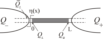
Figure 9: Disordered wire of symmetry class AIII connected to two normal terminals which are described by the Eilenberger functions $Q_{\pm}$. The $Q$-matrix at the boundaries between the wire and terminals is denoted by $Q_{L}$ and $Q_{R}$. The counter $\eta(x)$ which ’measures’ the parity current $j^{P}$ is located close to the left end of the wire.

The role of infinitesimal term which breaks the chiral symmetry is to provide the boundary conditions at infinities. The parity gauge field $A_{x}$ can be now eliminated at the expense of twisted boundary conditions in the left lead. Using the freedom in the choice of $A_{x}$ we set $A_{x}=\theta\times\eta^{\prime}(x)$, where $\eta(x)$ denotes any smooth step function on atomic scale at the crossection where the parity current is ’measured’ as shown in Fig. 9. Abbreviating by $\tilde{Q}_{L}=Q(-0)$ the Green’s function before the ’counter’ and by $Q_{L}=Q(+0)$ the one at the left end of the wire after the ’counter’, we see that the Eilenberger equation (224) yields

$$Q_{L}=e^{i\theta{\cal P}}\,\tilde{Q}_{L}\,e^{-i\theta{\cal P}}.$$ (225)

Let us also denote by $Q_{R}=Q(L)$ the Green’s function at the right end of the wire. It is related with the left configuration $Q_{L}$ by the transfer matrix,

$$Q_{R}=MQ_{L}M^{-1}.$$ (226)

This relation is central to the whole discussion. It obviates the need of solving the complicated Shrödinger equation with a disorder potential in the wire substituting the latter by the ‘black box’ characterized by the transfer matrix. As shown in Refs. [Nazarov and Blanter, 2009; Neven et al., 2013], the configurations $Q_{R,L}$ satisfy the following boundary conditions

$$(\mathds{1}+Q_{-})(\mathds{1}-\tilde{Q}_{L}) = 0,$$ (227)

$$(\mathds{1}-Q_{R})(\mathds{1}+Q_{+}) = 0,\qquad Q_{\pm}=\sigma_{3}^{RL}\otimes\mathds{1}^{\pm},$$

where $Q_{\pm}$ are asymptotic configurations. If one further expresses $\tilde{Q}_{L}$ in terms of $Q_{L}$, see Eq. (225), one arrives at the ’twisted’ boundary conditions,

$$\left(\mathds{1}+Q_{-}(\theta)\right)(\mathds{1}-Q_{L}) = 0,$$ (228)

$$(\mathds{1}-Q_{R})\left(\mathds{1}+Q_{+}\right) = 0.$$

We have introduced here the rotated asymptotic configuration at the left

$$\qquad Q_{-}(\theta) = e^{i\theta{\cal P}}\,\left(\sigma_{3}^{RL}\otimes\mathds{1}^{\pm}\right)\,e^{-i\theta{\cal P}}$$ (231)

$$= \left(\begin{array}[]{cc}\cos 2\theta&-i\hat{P}\sin 2\theta\\ i\hat{P}\sin 2\theta&-\cos 2\theta\end{array}\right)_{RL}$$

and used that ${\cal P}=\hat{P}\otimes\sigma_{1}^{RL}$. To proceed one can use the relation (226) and the new boundary conditions (228) in order to find the general expression for $Q_{R,L}$ in terms of the transfer matrix $M$ and asymptotic configurations $Q_{\pm}(\theta)$,

$$Q_{R} = \mathds{1}+\frac{2}{Q_{+}+MQ_{-}(\theta)M^{-1}}(\mathds{1}-Q_{+}),$$

$$Q_{L} = \mathds{1}+\left(\mathds{1}-Q_{-}(\theta)\right)\frac{2}{Q_{-}(\theta)+M^{-1}Q_{+}M}.\quad$$ (232)

The derivation of this result can be found in Ref. [Neven et al., 2013] and we do not repeat it here. The parity current when expressed in terms of $Q$-matrix becomes

$${\cal I}_{P}(\theta)=-\frac{1}{2}{\rm tr}\bigl{(}\hat{P}\sigma_{1}^{RL}Q_{L}\bigr{)}=-\frac{1}{2}{\rm tr}\bigl{(}\hat{P}\sigma_{1}^{RL}Q_{R}\bigr{)}$$ (233)

Since this current is conserved the result should not depend in which of the two terminals it is evaluated.

Our next goal is to relate ${\cal I}_{P}(\theta)$ with the Lyapunov exponents $\lambda_{n}$. We observe that $Q_{-}(\theta)$ can be factorized as $Q_{-}(\theta)={\cal R}\tilde{Q}_{-}(\theta){\cal R}$ where $\tilde{Q}_{-}(\theta)=e^{2i\theta\sigma_{1}^{\rm RL}}\,\sigma_{3}^{\rm RL}$ and ${\cal R}={\rm diag}(1,\hat{P})_{\rm RL}$. A similar decomposition holds for the transfer matrix if one takes into account Eq. (106), $M={\cal R}\tilde{M}{\cal R}$ with $\tilde{M}=Ve^{\lambda\sigma_{1}^{RL}}U^{\prime}$. We finally note that the parity operator in Eq. (233) can be represented as ${\cal P}=P\otimes\sigma_{1}^{\rm RL}={\cal R}\sigma_{1}^{\rm RL}{\cal R}$. Hence such factorization enables us to write ${\cal I}_{P}(\theta)=-\frac{1}{2}{\rm tr}\bigl{(}\sigma_{1}^{RL}\tilde{Q}_{L}\bigr{)},$ and the parity operator $\hat{P}$ acting in the sublattice space ($\pm$) can be dropped out from the subsequent manipulations. Noting that $\tilde{Q}_{-}(\theta)$ can be found via $\tilde{M}$ by means of the relation (232), with $M$ being substituted for $\tilde{M}$, and using the unitarity of matrices $V,U^{\prime}$, we find

$${\cal I}_{P}(\theta)=\sum_{k=1}^{N^{\prime}}\tanh\left(\lambda_{k}+i\theta\right).$$ (234)

Comparing now two definitions (VI) and (222), we can read off from here the generating function ${\cal F}(\phi_{0})=i{\cal I}_{P}(-i\phi_{0})$ and arrive to the result (110).

D.2 Class D

We outline here the proof of relations (108) and (115) for the class $\mathrm{D}$ disordered wire.

The way to derive the ’plus’ partition sum $Z^{(+)}(\phi)$, Eq. (108), is completely analogous to the one for chiral classes $\mathrm{AIII}$ and $\mathrm{BDI}$ considered above and we only sketch the main steps. The generator of the conserved symmetry current is given by $\tau_{1}^{\rm cc}$. Hence the Eilenberger equation corresponding to the gauge transformed Hamiltonian reads

$$i\partial_{x}Q(x)+\left[i0^{+}\,\sigma_{3}^{RL}\otimes\tau_{3}^{cc}+\tau_{1}^{\rm cc}A_{x},Q(x)\right]=0,$$ (235)

where we set $A_{x}=\theta\times\delta(x)$. At variance with $\mathds{Z}$-classes the $Q$-matrix here is defined in the direct product of the chiral- and the cc-spaces. The twisted asymptotic left configuration here assumes the form

$$Q_{-}(\theta)=\sigma_{3}^{RL}\otimes\left(e^{i\tau_{1}^{\rm cc}\theta}\tau_{3}^{cc}e^{-i\tau_{1}^{\rm cc}\theta}\right),$$ (236)

cf. with Eq. (231), while the right one reads $Q_{+}=\sigma_{3}^{RL}\otimes\tau_{3}^{cc}$ (the appearance of the matrix $\tau_{3}^{cc}$ here is rooted in the construction of the field integral for class $\mathrm{D}$ system, see sec. V.3). The generating function (VI) at the specific disorder realization can be further found from the relation ${\cal F}(\phi_{0})=(i/4){\rm tr}(\tau_{1}^{cc}Q_{L})\bigl{|}_{\theta=-i\phi_{0}}$ with the matrix $Q_{L}$ at the left end of the wire given by Eq. (232). When evaluating this expression one can use the fact that configurations $Q_{-}(\theta)$ and $Q_{+}$ have the trivial diagonal structure in the channel space. This means that the transfer matrix in Eq. (232) can be taken in the block-diagonal form by omitting $U$ and $V$ orthogonal rotations which mix the eigen-channels. In this way one arrives at the final result for the generating function depending only on the set of $\lambda$’s,

$${\cal F}(\phi_{0})=i\sum_{k=1}^{N^{\prime}}\frac{\sinh 2\phi_{0}}{\cosh 2\lambda_{k}+\cosh 2\phi_{0}},$$ (237)

in agreement with Ref. [Lamacraft et al., 2004]. It enables one to construct the bosonic partition sum using the relation $i\partial_{\phi_{0}}\ln Z_{B}^{(+)}(\phi_{0})={\cal F}(\phi_{0})$. Choosing the normalization ${\cal Z}_{B}^{(+)}(0)=1$, it can be cast into the form

$${\cal Z}^{(+)}_{B}(\phi_{0})=\prod_{k=1}^{N^{\prime}}\left(1+t^{2}_{k}\sinh^{2}\phi_{0}\right)^{1/2},\quad t_{k}=1/\cosh\lambda_{k},$$ (238)

from where the fermion partition sum follows as ${\cal Z}^{(+)}_{F}(\phi_{1})={\cal Z}^{(+)}_{B}(i\phi_{1})$. With the help of basic trigonometric identities one then finds for their ratio, ${\cal Z}^{(+)}(\phi)={\cal Z}^{(+)}_{F}(\phi_{1})/{\cal Z}^{(+)}_{B}(\phi_{0})$, the result (108).

Let us now evaluate the ‘minus’ partition function ${\cal Z}^{(-)}$. It was defined in sec. V.3 as a response of the system to the insertion of the $\mathds{Z}_{2}$ gauge ‘flux’ $\tau_{1}^{cc}$ on a single bond $(0,1)$. We have also stressed that the gauge transformation $\psi^{1}\to\tau_{1}\psi^{1},\bar{\psi}^{1}\to\bar{\psi}^{1}\tau_{1}$ can be used to shift such source to any other link. In particular, applying it to all cites $s$ with $s\leq 0$ the $\tau_{1}$-flux can be shifted to the left infinity. This transformation also changes the sign of the infinitesimal convergence factor in the fermionic sector of the path integral, $i0\,\tau_{1}^{cc}\to(-i0)\tau_{1}^{cc}$, which is important to keep in mind as long as one considers an open system (a wire connected to the left/right lead). On the level of Eilenberger equation this swaps the left asymptotic $Q$-matrix in the ff-sector, i.e. $Q_{-}=-\,Q_{+}=-\sigma_{3}^{RL}\otimes\tau_{3}^{cc}$. As one can now see from Eq. (236) such boundary conditions are equivalent to setting $\phi_{1}=\pi/2$ and thereby the identity (114) is proved.

D.3 Class DIII

Let us now extend the quasiclassical treatment introduced in the previous two sections to the class $\mathrm{DIII}$ system. In doing so we consider a more general model where impurity scattering is present not only in the wire but also in the leads. It will serve us twofold purpose. First, we will justify the general form of the grained action $S[T]$, see Eq. (95) or (191). Second, we will obtain the partition functions $Z^{(\pm)}(\phi)$ in terms of Lyapunov exponents using the action $S$ calculated for a specific choice of matrix $T$.

To this end we consider two dots or two leads (we refer them later as ‘terminals’), connected by a scattering region (‘junction’) which is assumed to be completely defined by its transfer matrix $\hat{M}$ obeying all required symmetries specific for the class $\mathrm{DIII}$, see Sec. VI for details. Depending on the situation, by the ’junction’ we understand the wire of a length $L$ itself or just a contact between two dots. For a given $\hat{M}$ we then perform a disorder averaging in the terminals in the framework of SCBA. Introducing further two matrices $T_{1,2}\in\mathrm{SpO}(2|2)$, which parametrize the Goldstone fluctuations in the terminals, and following the standard root outlined in Appendix A.2, one arrives at the following action

$$S[T_{1},T_{2}]=\frac{1}{2}{\rm str}\ln\left(\begin{array}[]{cc}i\Sigma_{0}\,\tau_{3}^{cc}\,T(x)&-D\\ -{D}^{\dagger}&i\Sigma_{0}T^{-1}(x)\,\tau_{3}^{cc}\end{array}\right),$$ (239)

Here $T(x)=T_{1,2}$ depending on whether $x$ lies in the L/R terminal, $\Sigma_{0}$ is the imaginary part of a SCBA self-energy ($\Sigma_{0}=0$ inside the junction), and the operator $D$ defined in Eq. (74) should be renormalized by the real part of a self-energy. The precise form of SCBA equations will not be important for the subsequent discussion. We only comment here that we imagine the SCBA scheme being performed separately for each terminal along the route of random matrix theory (RMT) approach Ivanov (2002), and adding afterwards an inter-grain non-random hopping matrix $W$ to the operator ${\cal D}$, see Eq. (75). By construction, the matrix $T$ enters the low-energy action as the element of the coset space $T=T^{-1}_{R}T_{L}$, see Eq. (76). In other words $T\in\mathrm{SpO}(2|2)\otimes\mathrm{SpO}(2|2)/\mathrm{SpO}(2|2)\simeq\mathrm{SpO}(2|2)$, thus the Goldstone manifold becomes isomorphic to the single copy of the group $\mathrm{SpO}(2|2)$.

Subjecting the Hamitonian $H$ to the gauge transform one obtains the phase dependent action $S_{\phi}[T_{1},T_{2}]$. It is given by Eq. (239) with the phase dependent Hamiltonian $H_{\phi}=H^{\prime}+W_{\phi}^{\prime}$ (we refer the reader to our previous discussion in Sec. V.7). By virtue of the gauge invariance the flux dependence can be removed from the junction to the left terminal, which yields

$$S_{\phi}[T_{1},T_{2}]=\frac{1}{2}{\rm str}\ln\left(\begin{array}[]{cc}i\Sigma_{0}\tau_{3}^{cc}\,T_{\phi}(x)&-D^{\prime}\\ -{D^{\prime}}^{\dagger}&i\Sigma_{0}T^{-1}_{\phi}(x)\,\tau_{3}^{cc}\end{array}\right),$$ (240)

where the rotated field $T_{\phi}(x)$ is defined as

$$T_{\phi}(x)=e^{-i\tau_{3}^{cc}\phi(x)}T(x)e^{-i\tau_{3}^{cc}\phi(x)},$$ (241)

with $\phi(x)={\rm diag}(-i\phi_{0},\phi_{1})_{\rm bf}$ if $x$ belongs to the left terminal and $\phi(x)=0$ otherwise. Let us also denote by

$$T_{1}(\phi)=e^{-i\tau_{3}^{cc}\phi}\,T_{1}e^{-i\tau_{3}^{cc}\phi}=T_{\phi}(x)\bigl{|}_{x\in L}$$ (242)

the rotated configuration in the left terminal.

In fact, the action $S_{\phi}[T_{1},T_{2}]$ depends only on the group element $T_{12}=T_{1}(\phi)T_{2}^{-1}$ but not on each of the two fields separately. To see that we introduce the Green’s function ${\cal G}_{\phi}[T_{1},T_{2}]$ such that $S_{\phi}=\frac{1}{2}{\rm str}\ln{\cal G}^{-1}_{\phi}$ and subject the former to a global similarity transformation,

$$G^{-1}_{\phi}=\left(\begin{array}[]{cc}\tau_{3}^{cc}&\\ &T_{2}\end{array}\right){\cal G}^{-1}_{\phi}\left(\begin{array}[]{cc}T^{-1}_{2}&\\ &\tau_{3}^{cc}\end{array}\right),$$ (243)

which preserves the structure of the action since the rotations involved have unit super-determinant. Explicitly, the transformed Green’s function takes the form

$$G_{\phi}[T_{12}]=\left(\begin{array}[]{cc}i\Sigma_{0}\,T_{12}(x)&-D^{\prime}\\ -D^{\prime\dagger}&i\Sigma_{0}\,T_{12}^{-1}(x)\end{array}\right)^{-1},$$ (244)

with $T_{12}(x)$ being the step-like in space field defined by relations $T_{12}(x)|_{x\in R}=\mathds{1}$ and $T_{12}(x)|_{x\in L}=T_{12}$. The above form (244) of the Green’s function is valid in the chiral basis where the parity operator $P=\sigma_{3}$. It is advantageous to rewrite $G_{\phi}$ in the basis independent form. Introducing the (step-like) element $\hat{\Omega}(x)=-i\ln T_{12}(x)$ from the Lie superalgebra $\mathfrak{g}=\mathfrak{gl}(2|2)$ one obtains

$$G_{\phi}[T_{12}]=\left(\hat{\Sigma}(x)-H\right)^{-1},$$

$$\hat{\Sigma}(x)=i\Sigma_{0}\exp\{2iP\otimes\hat{\Omega}(x)\}.$$ (245)

We have used here that $P^{2}=\mathds{1}$ and matrices $P$ and $\Omega$ act in different subspaces.

To evaluate the action $S_{\phi}[T_{12}]=\frac{1}{2}\ln{\rm Sdet}\,G_{\phi}[T_{12}]$ we introduce the auxiliary parameter $t\in[0,1]$ and define the field $T_{12}^{t}(x)=e^{it\hat{\Omega}(x)}$. By rescaling the algebra element $\Omega$ in Eq. (D.3) in the same way one obtains the $t$-dependent Green’s function $G_{\phi}[T_{12}^{t}]$ and the action $S_{\phi}[T_{12}^{t}]$, where $T_{12}^{t}=T_{12}^{t}(x)|_{x\in L}$ is the $T$-field in the left terminal. Our subsequent strategy to find this new action will be the same as for other symmetry classes. First of all, using the quasiclassical approach, we find the average $t$-dependent symmetry current ${\cal I}_{\Omega}(t)$, and later on with the help of this current reconstruct the action. To this end we put the gauge source on the link $0\leftrightarrow 1$ (it can be thought of as the boundary between the left terminal and the junction) by changing the corresponding hopping matrix,

$$W^{\prime}\to W^{\prime}_{t}=\left(\begin{array}[]{cc}&e^{it\hat{\Omega}}w^{\prime}\\ w^{\prime\dagger}e^{it\hat{\Omega}}&\end{array}\right),$$ (246)

where $\hat{\Omega}=\hat{\Omega}(x)|_{x\in L}=-i\ln T_{21}$ is the ‘angle’ in the left terminal. We use it to define the average symmetry current according to the relation

$${\cal I}_{\Omega}(t):=i\partial_{t}S_{\phi}[T_{12}^{t}]=-\frac{i}{2}{\rm str}\Bigl{(}(\partial_{t}H_{t})\bigl{|}_{t=0}\,G_{\phi}[T_{12}^{t}]\Bigr{)},$$ (247)

with $H_{t}=H^{\prime}+W^{\prime}_{t}$. The first equality here is a definition and the second one follows from the gauge invariance.

Following the logic of the quasiclassical approach let us now linearize the Hamitonian in the terminals around zero energy, $H\to{\cal H}_{L,R}$, and reduce the equation of motion for the Green’s function $G_{\phi}[T_{12}^{t}]$ to the Eilenberger equation. In the Majorana basis one has ${\cal H}_{L,R}=-iv\sigma_{3}^{RL}\otimes\mathds{1}^{cc}\,\partial_{x}$, and the definition of Eilenberger $Q$-function is given by Eq. (223). The Eilenberger equation (235) itself is get modified because of the presence of the self-energy in the terminals and takes the form

$$i\partial_{x}Q(x)+i(\Sigma_{0}/v)\,\left[\hat{\Xi}(x),Q(x)\right]=0,$$ (248)

where ${\cal P}=P\otimes\sigma_{1}^{RL}$ is the parity operator and

$$\hat{\Xi}(x)=\sigma_{3}^{RL}\,e^{2it{\cal P}\otimes\hat{\Omega}(x)}=e^{-it{\cal P}\otimes\hat{\Omega}(x)}\sigma_{3}^{RL}e^{it{\cal P}\otimes\hat{\Omega}(x)}.$$ (249)

The last representation here is valid since $\{{\cal P},\sigma_{3}^{RL}\}_{+}=0$. The presence of $\sigma_{3}^{RL}$ Pauli matrix in the self-energy $\hat{\Xi}$ stems from the original definition of the $Q$-matrix (223) and leads to the normalization $\hat{\Xi}^{2}(x)=\mathds{1}$. It is clear that the matrix $\hat{\Xi}$ will fix the $t$-dependent boundary conditions in the terminals for such Eilenberger equation,

$$Q_{-}(t)=e^{-it{\cal P}\otimes\hat{\Omega}}\sigma_{3}^{RL}e^{it{\cal P}\otimes\hat{\Omega}},\qquad Q_{+}=\sigma_{3}^{RL}.$$ (250)

With this understanding we proceed further with the evaluation of a symmetry current ${\cal I}_{\Omega}(t)$ in terms of the field $T_{12}^{t}$ and the Lyapunov exponents $\lambda_{k}$. The quasiclassical approximation of the lattice representation (247) for this current has the form

$${\cal I}_{\Omega}(t)=-\frac{1}{2}{\rm str}\bigl{(}({\cal P}\otimes\hat{\Omega})\,Q_{L}\bigr{)},$$ (251)

with $Q_{L}$ being the Green’s function (232) right at the boundary of the left terminal and the junction. We note that the SCBA self-energy $\Sigma_{0}$ does not enter into $Q_{L}$ and $Q_{R}$. In analogy with $\mathds{Z}$-class calculations we observe that the configuration $Q_{-}(t)$ admits the factorization $Q_{-}(t)={\cal R}\,\tilde{Q}_{-}(t){\cal R}$ where $\tilde{Q}_{-}(t)=\sigma_{3}^{\rm RL}e^{2i(\sigma_{1}^{RL}\otimes\hat{\Omega})t}$ and ${\cal R}={\rm diag}(1,\hat{P})_{\rm RL}$. The transfer matrix $M$ can be put in the same form if one takes into account its DMPK decomposition (106) and the class $\mathrm{DIII}$ symmetries of the rotation matrices, cf. Sec. VI for these details. We thus write $M={\cal R}\tilde{M}{\cal R}$ where $\tilde{M}=Ve^{\lambda P\sigma_{1}^{RL}}U^{\prime}$. We finally note that the symmetry current generator in Eq. (251) can be represented as ${\cal P}\otimes\hat{\Omega}=P\otimes\sigma_{1}^{\rm RL}\otimes\hat{\Omega}={\cal R}(\sigma_{1}^{\rm RL}\otimes\hat{\Omega}){\cal R}$. Thereby we are able to write ${\cal I}_{\Omega}(t)=\frac{1}{2}{\rm str}\bigl{(}(\sigma_{1}^{RL}\otimes\hat{\Omega})\,\tilde{Q}_{L}\bigr{)}$, where $\tilde{Q}_{L}$ has to be found using Eq. (232), with $M$ being changed to $\tilde{M}$ and $Q_{-}(\theta)$ being changed to $\tilde{Q}_{-}(t)$. Obviously, the orthogonal rotations $V$ and $U^{\prime}$ do not enter the final result for the current. Proceeding in basis where $P$ is diagonal we obtain

$${\cal I}_{\Omega}(t)=\frac{1}{2}\sum_{\sigma=\pm}\sum_{k=1}^{N^{\prime}/2}{\rm str}\Bigl{(}\hat{\Omega}\tanh\left(\sigma\lambda_{k}-i\hat{\Omega}t\right)\Bigr{)}.$$ (252)

The sum over index $\sigma$ is due to $\pm 1$ eigenvalues of the parity operator $P$ and the sum over $k$ extends over the set of Lyapunov exponents without taking into account their Kramers degeneracy. Using trigonometry this result can be cast into the form

$${\cal I}_{\Omega}(t)=-\frac{1}{2}\sum_{k=1}^{N^{\prime}}{\rm str}\left(\frac{i\hat{\Omega}\sin(2\hat{\Omega}t)}{\cosh 2\lambda_{k}+\cos(2\hat{\Omega}t)}\right),$$ (253)

which is of the same type as our preceding class $\mathrm{D}$ result (237). From here the action is found via relation $S_{\phi}[T_{12}]=-i\int_{0}^{1}dt\,{\cal I}_{\Omega}(t)$ that yields

$$S_{\phi}[T_{12}]=\frac{1}{4}\sum_{k=1}^{N^{\prime}}{\rm str}\ln\left(\openone-t_{k}^{2}\sin^{2}\hat{\Omega}\right).$$ (254)

With the help of ansatz

$$4\sin^{2}\hat{\Omega}=2(1-\cos 2\hat{\Omega})=2-T_{1}(\phi)T_{2}^{-1}-T_{2}T_{1}^{-1}(\phi)$$

the final form of the action reads

$$S_{\phi}[T_{12}]=$$ (255)

$$\quad{1\over 4}\sum\limits_{k=1}^{N^{\prime}}\mathrm{str}\ln\left[\openone+\frac{t_{k}^{2}}{4}\left(T_{1}(\phi)T_{2}^{-1}+T_{2}T_{1}^{-1}(\phi)-2\right)\right],$$

cf. Eq. (95).

With this result the evaluation of the partition functions $Z^{\pm}=e^{-S^{\pm}}$ becomes particularly simple. Setting $T_{1}=T_{2}=\openone$ and keeping a non-vanishing angle $\phi$ one obtains the relation (108). On other hand, the choice $T_{1}={\cal P}^{\mathrm{b}}+{\cal P}^{\mathrm{f}}\tau_{1}^{cc}$ and $T_{2}=\openone$ gives the desired result (115) for the kink’s action.

References

- Note (1) We here consider a topological superconductor as a thermal insulator, i.e. our usage of the term ‘insulator’ encompasses both conventional insulators, and superconductors.
- Hasan and Kane (2010) M. Z. Hasan and C. L. Kane, Rev. Mod. Phys. 82, 3045 (2010).
- Bernevig and Hughes (2013) B. A. Bernevig and T. L. Hughes, Topological Insulators and Topological Superconductors (Princeton Press, 2013).
- Note (2) As a matter of principle, the momentum space description can be maintained at the expense of extending the unit cell from atomistic scales, , to the system size, (a disordered system is periodic in its own size.) However, the price to be payed is that the topological information is now encoded in the configuration dependent structure of bands. While the multi-band framework may still be accessible by numerical means, it is less suited for analytical theory building.
- Prange (1981) R. Prange, Physical Review B 23, 4802 (1981).
- Khmelnitskii (1983) D. E. Khmelnitskii, JETP Lett. 38, 552 (1983).
- Abrahams et al. (1979) E. Abrahams, P. W. Anderson, D. C. Licciardello, and T. V. Ramakrishnan, Phys. Rev. Lett. 42, 673 (1979).
- Pruisken (1984) A. Pruisken, Nucl. Phys. B 235, 277 (1984).
- Levine et al. (1984) H. Levine, S. B. Libby, and A. M. M. Pruisken, Nucl. Phys. B 240, 30 (1984).
- Gruzberg et al. (1999) I. Gruzberg, A. Ludwig, and N. Read, Phys. Rev. Lett. 82, 4524 (1999).
- Senthil et al. (1999) T. Senthil, J. B. Marston, and M. P. A. Fisher, Phys. Rev. B 60, 4245 (1999).
- Brouwer et al. (2000a) P. Brouwer, C. Mudry, and A. Furusaki, Nucl. Phys. B 565, 653 (2000a).
- Brouwer et al. (2000b) P. W. Brouwer, A. Furusaki, I. A. Gruzberg, and C. Mudry, Phys. Rev. Lett. 85, 1064 (2000b).
- Gruzberg et al. (2005) I. Gruzberg, N. Read, and S. Vishveshwara, Phys. Rev. B 71, 245124 (2005).
- Brouwer et al. (1998) P. W. Brouwer, C. Mudry, B. D. Simons, and A. Altland, Phys. Rev. Lett. 81, 862 (1998).
- Motrunich et al. (2001) O. Motrunich, K. Damle, and D. Huse, Phys. Rev. B 63, 224204 (2001).
- Groth et al. (2009) C. Groth, M. Wimmer, A. Akhmerov, J. Tworzydło, and C. Beenakker, Phys. Rev. Lett. 103, 196805 (2009).
- Rieder et al. (2013) M.-T. Rieder, P. W. Brouwer, and I. Adagideli, Phys. Rev. B 88, 060509 (2013).
- Fu and Kane (2012) L. Fu and C. L. Kane, Phys. Rev. Lett. 109, 246605 (2012).
- König et al. (2012) E. J. König, P. M. Ostrovsky, I. V. Protopopov, and A. D. Mirlin, Phys. Rev. B 85, 195130 (2012).
- Mathur (1997) H. Mathur, Phys. Rev. B 56, 15794 (1997).
- Bocquet et al. (2000) M. Bocquet, D. Serban, and M. Zirnbauer, Nucl. Phys. B 578, 628 (2000).
- Howe (1989) R. Howe, Trans. Amer. Math. Soc. 313, 539 (1989).
- Cheng and Wang (2012) S.-j. Cheng and W. Wang, Dualities and Representations of Lie Superalgebras (American Mathematical Society, 2012).
- Haldane (1983) F. Haldane, Phys. Lett. A 93, 464 (1983).
- Su et al. (1979) W. P. Su, J. R. Schrieffer, and A. J. Heeger, Phys. Rev. Lett. 42, 1698 (1979).
- Nazarov (1994) Y. Nazarov, Phys. Rev. Lett. 73, 134 (1994).
- Lamacraft et al. (2004) A. Lamacraft, B. Simons, and M. Zirnbauer, Phys. Rev. B 70, 075412 (2004).
- Altland and Merkt (2001) A. Altland and R. Merkt, Nucl. Phys. B 607, 511 (2001).
- Note (3) There exists one more term, , which, however, does not play an essential role in the present contextAltland and Merkt (2001).
- Efetov (1997) K. B. Efetov, Supersymmetry in Disorder and Chaos (Cambridge University Press, 1997).
- Note (4) There is a subtlety here. The boundary condition implies describes the functional integral upon approaching zero length. This is a ‘zero-dimensional’ -function, in the sense that it does not contain a divergent pre-factor . In particular, it does not contribute to the spectral decomposition of the function .
- Altland et al. (2014) A. Altland, D. Bagrets, L. Fritz, A. Kamenev, and H. Schmiedt, Phys. Rev. Lett. 112, 206602 (2014).
- Mondragon-Shem et al. (2014) I. Mondragon-Shem, J. Song, T. L. Hughes, and E. Prodan, Phys. Rev. Lett. 113, 046802 (2014).
- Ivanov (2002) D. A. Ivanov, J. Math. Phys. 43, 126 (2002).
- Verbaarschot and Zahed (1993) J. J. M. Verbaarschot and I. Zahed, Phys. Rev. Lett. 70, 3852 (1993).
- Note (5) In the cases, we will be led to non-trivial connections, i.e. the placement of a single Ising like kink into a circular structure, a configuration that clearly would not work on a trivial product space (on which only even numbers of kinks are permissible.) In these cases, the gauge flux simply is the number of kinks mod 2.
- Kitaev (2001) A. Y. Kitaev, Physics-Uspekhi 44, 131 (2001).
- Zirnbauer (1996) M. R. Zirnbauer, J. Math. Phys. 37, 4986 (1996).
- Mirlin et al. (1994) A. D. Mirlin, A. Müller-Groeling, and M. R. Zirnbauer, Annals of Physics 236, 325 (1994).
- Helgason (1984) S. Helgason, Groups and Geometric Analysis (Academic Press, 1984).
- Fulga et al. (2011) I. C. Fulga, F. Hassler, A. R. Akhmerov, and C. W. J. Beenakker, Phys. Rev. B 83, 155429 (2011).
- Fulga et al. (2012) I. C. Fulga, F. Hassler, and A. R. Akhmerov, Phys. Rev. B 85, 165409 (2012).
- Note (6) To see it explicitly let us represent , with being the Hamiltonian of the auxiliary system with the deleted single bond and is the hopping matrix on this bond. Then the fermionic action with the inserted source reads , where we have used . We can now apply the orthogonal rotation in the ’charge-conjugation’ space to the spinor in order to transform the action into the form with being the Hamiltonian of the system with a sign inversion on the bond . All Grassmann fields in the rotated spinor are independent. Hence, performing the Gaussian integration we find that the modified fermion partition sum reads .
- Nazarov and Blanter (2009) Y. V. Nazarov and Y. M. Blanter, Quantum Transport (Cambridge University Press, 2009).
- Kamenev (2011) A. Kamenev, Field Theory of Non-Equilibrium systems (Cambridge University Press, 2011).
- Grover et al. (2014) T. Grover, D. N. Sheng, and A. Vishwanath, Science 344, 280 (2014).
- Barut et al. (1987) A. O. Barut, A. Inomata, and R. Wilson, J. Phys. A 20, 4083 (1987).
- Bagrets and Altland (2012) D. Bagrets and A. Altland, Phys. Rev. Lett. 109, 227005 (2012).
- Zirnbauer (1994) M. R. Zirnbauer, Annalen der Physik 506, 513 (1994).
- Mildenberger et al. (2007) A. Mildenberger, F. Evers, A. D. Mirlin, and J. T. Chalker, Phys. Rev. B 75, 245321 (2007).
- Neven et al. (2013) P. Neven, D. Bagrets, and A. Altland, New Journal of Physics 15, 055019 (2013).