Flat histogram quantum Monte Carlo for analytic continuation to real time

Abstract

The Quantum Monte Carlo (QMC) method can yield the imaginary-time dependence of a correlation function $C(\tau)$ of an operator $\hat{O}$. The analytic continuation to real-time proceeds by means of a “numerical inversion” of these data to find the response function or spectral density $A(\omega)$ corresponding to $\hat{O}$. Such a technique is very sensitive to the statistical errors in $C(\tau)$ especially for large values of $\tau$, when we are interested in the low-energy excitations. In this paper, we find that if we use the flat histogram technique in the QMC method, in such a way to make the histogram of $C(\tau)$ flat, the results of the analytic continuation for low-energy excitations improve using the same amount of computational time. To demonstrate the idea we select an exactly soluble version of the single-hole motion in the $t-J$ model and the diagrammatic Monte Carlo technique.

I Introduction

Quantum Monte Carlo simulation, an undeniably useful tool in addressing a number of issues in quantum many-body physics, cannot be used to simulate real-time dynamics. By means of analytic continuation to Euclidean time $\tau$ ($t\to-i\tau$), however, the Schrödinger equation turns into a diffusion equation, which can be simulated using random walks which explore the potential landscape by spending proportionately more “time” near the valleys of the potential and less “time” near the potential heights. The same transformation into imaginary time turns the path integral representation of the evolution operator from an integral over paths of computationally “nasty” phase factors, a problem almost impossible to treat stochastically, into an integral over paths in imaginary time weighted by a real and positive “Boltzmann-like” weight; this weight is interpreted as a well-behaved probability for a particular path to contribute to the sum and this interpretation allows a straightforward stochastic treatmentCeperley (1995).

This transformation, by itself, is useful because it yields the interacting ground state and physical quantities related to the equilibrium statistical mechanical description of a quantum many-body system. However, if we are interested in obtaining information about the real-time dynamics and information about the excitations of the system, an “inversion” of this ill-defined transformation for the results of correlation functions $C(\tau)$ of an operator $\hat{O}$ representing a physical observable, namely,

$$C(\tau)=\langle\hat{T}_{\tau}\hat{O}(\tau)\hat{O}^{\dagger}(0)\rangle,$$ (1)

(where $\hat{T}_{\tau}$ is the imaginary-time ordering operator) from the imaginary time $\tau$ back to real time $t$ is required.

The analytic continuation to real-time proceeds by means of a “numerical inversion” of the QMC data on $C(\tau)$ to find the spectral function $A(\omega)$. These inversion techniques, such as the so-called maximum entropy methodJarrell and Gubernatis (1996) or its generalization, the so-called stochastic analytical inference (SAI) methodFuchs et al. (2010); Beach (2004), require very accurate QMC data on $C(\tau)$. Since collective phenomena emerge at energy scales significantly smaller than the typical short-range interaction energy scale, we are mainly interested in sampling the long imaginary part of such response or correlation functions. Such response functions obtained by QMC are noisy data and in a limited $\tau$ range. If we are interested in extracting the low energy excitations, this information hides more clearly in the long-imaginary-time evolution of the correlation functions which is typically obscured by statistical errors.

Flat histogram methods have been very useful in classical systemsBerg and Newhaus (1991); Wang and Landau (2001a, b); de Oliviera et al. (1996) to overcome problems in simulations of first order phase transitions, systems with rough energy landscapes, etc. The flat histogram idea has been extended in quantum many-body systems and, in particular, in stochastic series expansionTroyer et al. (2003) to overcome the tunneling problem in first order phase transitions, in the continuous-time quantum Monte Carlo approach to the impurity solver problem used in dynamical mean-field-theory DMFTGull et al. (2011) and the diagrammatic Monte Carlo methodDiamantis and Manousakis (2013).

The main idea presented in this paper, in simple terms, is the following. We show that the flat-histogram method can be applied to the QMC method itself to make the histogram of $C(\tau)$ flat for all $\tau$ by sampling the variable $\tau$, and keeping track of the factors in each imaginary-time interval needed to achieve this result. In this way, we are able to compute $C(\tau)$ in a greater $\tau$ range with significantly smaller stochastic error. This approach allows us to achieve greater degree of accuracy when inverting the information contained in $C(\tau)$ to find its corresponding spectral function $A(\omega)$ in the entire range of values of $\omega$ of our interest.

In order to demonstrate the idea in the present paper, we need to make specific choices of i) a non-trivial quantum many-body problem, ii) a specific QMC method, iii) a specific correlation function $C(\tau)$, and iv) a method to carry out the analytic continuation. Using the same methods and techniques we will calculate the spectral function $A(\omega)$ using QMC with and without the application of the flat histogram method during the QMC runs which produce the data on $C(\tau)$. We will show that the flat histogram QMC method is superior to a simple QMC approach in which no flat histogram ideas have been implemented for such important observables. Using our past specific experience with models and QMC techniques, we choose the problem of the Green’s function $G_{\vec{k}}(\tau)$ of a single hole in the $t-J$ modelLiu and Manousakis (1991, 1992) with the diagrammatic Monte Carlo (DMC) methodProkof’ev and Svistunov (1998); Mishchenko et al. (2000); Diamantis and Manousakis (2013) using the method of the stochastic analytical inferenceFuchs et al. (2010) for the analytic continuation to obtain the spectral function $A_{\vec{k}}(\omega)$ from the QMC data obtained for $G_{\vec{k}}(\tau)$.

We apply the flat histogram idea with the combination of the DMC method and the Wang-Landau method, which we will refer to as the flat histogram diagrammatic Monte Carlo (FHDMC) methodDiamantis and Manousakis (2013). We will also use the standard implementation of the DMCProkof’ev and Svistunov (1998); Mishchenko et al. (2000) where a guidance function is used when sampling $G_{\vec{k}}(\tau)$. In the latter case, as we will see, the use of a parameter $\mu$ effectively makes the histogram of $G_{\vec{k}}(\tau)$ flat. On the other hand, we will also carry out DMC simulations using $\mu=0$ without the application of the flat histogram idea, which we will refer to as DMC0 which yields a histogram of $G_{\vec{k}}(\tau)$ very far from being flat, and we compare these results with those obtained with above two QMC methods, i.e., with standard-DMC and FHDMC. This comparison is made in order to show the main point of our paper that if the flat histogram idea is incorporated in any QMC method, it will provide a more accurate analytic continuation to real time.

The paper is organized as follows. In Sec. II we describe the problem, the model, and the general approach which we will follow. Sec. III describes the computational details and our implementation of the analytic continuation technique which we adopted. In Sec. IV we present the results of the spectral function obtained with the DMC0, the standard DMC, and FHDMC method, which are compared to what we believe to be the “exact” results of a soluble but restricted version of the $t-J$ model. Lastly, in Sec. V we present the main conclusions of the paper.

II The method

In order to be precise we take the example where the operator $\hat{O}^{\dagger}$ is the single particle creation operator $a^{\dagger}_{\vec{k}}$, in which case $C(\tau)$ becomes the single particle Green’s function $G_{\vec{k}}(\tau)$ in imaginary time. In this case the spectral function $A_{\vec{k}}(\omega)$ is related to $G$ as follows

$$G_{\vec{k}}(\tau)=\int d\omega K(\tau,\omega)A_{\vec{k}}(\omega),$$ (2)

where the so-called kernel $K(\tau,\omega)$ is simply $e^{-\omega\tau}$. The spectral function is a non-negative quantity normalized to unity.

We consider a finite imaginary time range, $0<\tau<\tau_{max}$ and we divide it into $L$ equal intervals. By integrating Eq. 2 in each time interval $i$ we obtain

$${\cal G}_{\vec{k}}(i) = \int d\omega{\bar{K}}(i,\omega)A_{\vec{k}}(\omega),$$ (3)

$${\cal G}_{\vec{k}}(i) \equiv {1\over{\Delta\tau_{i}}}\int_{\tau_{i-1}}^{\tau_{i}}G_{\vec{k}}(\tau)d\tau,$$ (4)

and ${\bar{K}}(i,\omega)$ is the average value of the kernel $K(\tau,\omega)=e^{-\omega\tau}$ in the $i$ interval, i.e., ${\bar{K}}(i,\omega)={{e^{-\omega\tau_{i}}}\over{\omega\Delta\tau_{i}}}[e^{\omega\Delta\tau_{i}}-1]$.

In Ref. Diamantis and Manousakis, 2013, we have shown that we can apply the flat histogram technique on the so-called diagrammatic Monte Carlo methodProkof’ev and Svistunov (1998); Mishchenko et al. (2000, 2001); Mishchenko and Nagaosa (2004, 2006); Cataudella et al. (2007) to make the histogram ${\cal G}_{\vec{k}}(i)$ of $G_{\vec{k}}(\tau)$ flat. The idea was demonstrated on the Fröhlich polaron problem. The results of the flat histogram DMC (FHDMC) on the estimate for the polaron ground state were significantly better than the result of the DMC0. However, as argued in the paperDiamantis and Manousakis (2013) the polaron problem spectrum was characterized by a gap, and the full advantage of the flat histogram method over DMC0 could not fully demonstrated.

In the present paper we use a simplified version of the $t-J$ model, in which the Heisenberg and the hole-hopping terms are linearized within the spin-wave approximation to obtain a polaron-like HamiltonianKane et al. (1989); Liu and Manousakis (1992), i.e.,

$$\hat{H} = -\sum_{\vec{k},\vec{q}}g(\vec{k},\vec{q})a^{\dagger}_{\vec{k}+\vec{q}}a_{\vec{k}}b_{\vec{q}}+H.c.$$ (5)

$$+ \sum_{\vec{k}}\hbar\omega(k)b^{\dagger}_{\vec{k}}b_{\vec{k}},$$

$$g(\vec{k},\vec{q}) = {{4t}\over{\sqrt{N}}}(u_{\vec{q}}\gamma_{\vec{k}-\vec{q}}+v_{\vec{q}}\gamma_{\vec{k}}),$$ (6)

$$\gamma_{\vec{k}} = -2t(\cos(k_{x}a)+\cos(k_{y}a)),$$ (7)

where the operator $b^{\dagger}_{\vec{q}}$ is the Bogoliubov spin-wave creation operator, $\omega(k)$ is the spin-wave dispersion of the square lattice quantum antiferromagnetManousakis (1991) and $a^{\dagger}_{\vec{k}}$ is the hole creation operator. Here $g(\vec{k},\vec{q})$ is the coupling of the hole to spin waves and $u_{\vec{k}}$ and $v_{\vec{k}}$ are the coefficients of the the Bogoliubov transformation as given in Ref. Manousakis, 1991

The single-hole spectral function of the above Hamiltonian can be approximated by the non-crossing approximation(NCA)Kane et al. (1989); Liu and Manousakis (1991, 1992). The diagrammatic Monte Carlo (DMC) method with or withoutMishchenko et al. (2001); Mishchenko and Nagaosa (2004, 2006); Cataudella et al. (2007) the incorporation of the flat histogram technique can be applied to the problem of a single-hole. In this paper in order to demonstrate the method, we wish to restrict our DMC to the sampling of only the diagrams contributing to the NCA. This restriction is actually a more difficult approach to numerically implement than the one in which the Markov process samples all the connected diagrams contributing to $G_{\vec{k}}(\tau)$. The reason for restricting ourselves within the NCA diagrammatic space, is because in this case there is an “exact” solution to the problem which we can use to measure the success of the approach discussed here. In order to obtain the “exact” solution, we have recalculated the single-hole Green’s function within the NCA approach described in Ref. Liu and Manousakis, 1992 for $\vec{k}=(\pi/2,\pi/2)$ for a $32\times 32$ size square lattice and a finite imaginary part was used in the free-hole propagator with $\epsilon=0.002$ (in units of the hopping parameter $t$) which smears the lowest energy quasiparticle peak. Note that as discussed in Ref. Liu and Manousakis, 1992 on this size lattice the finite-size effects were found to be small. The results of these calculations will be used as default models and we will refer to them as “exact” solutions.

We have applied the DMC0, the standard DMC, and FHDMC methods to obtain $G_{\vec{k}}(\tau)$ for $\vec{k}=(\pi/2,\pi/2)$ and $J/t=0.2$ in the NCA restricted diagrammatic space. We have carried out QMC simulations for a range of $J/t$ to compare with the exact results in order to make sure that our computer programs are correct.

Now imagine that we obtain a set of data $G^{(d)}_{\vec{k}}(i,j)$ $i=1,...,L$, $j=1,...,N_{d}$ on ${\cal G}_{\vec{k}}(i)$ obtained by any of the previously discussed three different QMC methods, where the $j$ denotes the data bin. For the analytic continuation we will use a generalization of the maximum entropy method, the so-called stochastic analytical inference (SAI) technique. In the later approach, $A_{\vec{k}}(\omega)$ is obtained as the average over all its possible forms in a Monte Carlo integration where the particular form of $A_{\vec{k}}(\omega)$ is selected from a distribution determined by the so-called default model $D_{\vec{k}}(\omega)$ and the probability of any proposed form of $A_{\vec{k}}(\omega)$ to be the true form given the input data $G^{(d)}_{\vec{k}}(i,j)$ is given by

$$P[A/G^{(d)}_{\vec{k}}] \sim e^{-{{\chi^{2}[A]}\over{2\alpha}}},$$ (8)

where $\chi^{2}[A]$ is the $\chi^{2}$ determined from the data $G^{(d)}_{\vec{k}}(i,j)$ on ${\cal G}_{\vec{k}}(i)$ and the result which is obtained from Eq. 2 using the proposed form of $A_{\vec{k}}(\omega)$. In the evaluation of $\chi^{2}[A]$ the covariance matrix of the data is used. The technical details of how one selects the particular proposed $A_{\vec{k}}(\omega)$ according to a given default model $D(\omega)$ and other important details of this calculation are discussed in Sec. III.

In the process of the analytic continuation we will analyze the QMC data obtained with the three different QMC methods which we discussed above. Namely, first we will use DMC0 approach in which no guidance function has been implemented (i.e., $\mu=0$). Second, we will use data obtained by means of standard-DMC (SDMC) where the histogram of $G(\tau)$ is made approximately flat by multiplying $G(\tau)$ with an exponential “guidance” function (we use the same terminology used in Ref. Prokof’ev and Svistunov (1998)) of the form $\exp(\mu\tau)$. In Fig. 1(a) we compare the histograms of $G(\tau)$ obtained with both DMC0 and standard-DMC. It is clear that the standard DMC makes the histogram of $G(\tau)$ approximately flat. Therefore, we will consider this method as an approximately flat histogram approach. Last, we will also use data obtained by the FHDMC. Notice that the histogram of $G(\tau)$ which we obtain using the Wang-Landau algorithm is flat to better than $95\%$.

Furthermore, we will use three different default models in each of the above cases, i.e., the total number of results presented will correspond to nine combinations of QMC data and default models. In one series of results presented in this paper, we will use as default model the “exact” solution to the problem. As a second choice for default model we will use a flat distribution, and as a third choice we will use a default model which shares some aspects of the “exact” solution but it differs significantly from the “exact” solution and we call it the “incorrect” default model. These three choices are discussed in Sec. III.2 in detail.

III Computational Details

As discussed in the previous Section, we will restrict our DMC approach to sample the diagrammatic subspace spanned only by the diagrams included in the non-crossing approximationKane et al. (1989); Liu and Manousakis (1991, 1992). The only reason for this restriction is that the problem of the single-hole spectral function can be solved “exactly” (“exact” with the limitations discussed in the previous Section) and, this, can be used to test the accuracy of the results of QMC method.

Furthermore, we will work with three sets of QMC data obtained for the histogram of $G_{\vec{k}}(\tau)$ for $\vec{k}=(\pi/2,\pi/2)$ and $J/t=0.2$. One set is obtained with DMC0, the second set is obtained with standard DMC, and the third set is obtained with FHDMC; all three sets of data are obtained with approximately the same amount of CPU time in order to compare. The first set of data for the histogram of $G_{\vec{k}}(\tau)$ is obtained for $0<\tau<3.8$ (in units of the inverse hopping matrix element $t$) while the other two sets of data are obtained for $0<\tau<12$ and in all three sets of data we have used 600 $\tau$-intervals ($L=600$) and the number of data bins $N_{d}=1200$ for each time-interval. In Fig. 1(a) we show that the histogram of $G(\tau)$ obtained by the standard DMC is fairly flat over a very wide range of $\tau$ while that of the DMC0 is approximately an exponentially increasing function of $\tau$. Therefore, we will consider that the standard DMC method is a method which produces an approximately flat histogram.

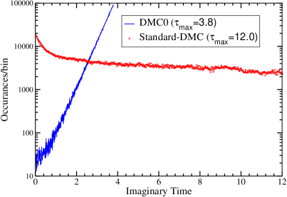
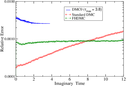
Figure 1: (Color on-line) (a) Our results for the histogram of $G_{\vec{k}}(\tau)$ (with $\vec{k}=(\pi/2,\pi/2)$) as a function of the imaginary time as obtained with the standard-DMC and the DMC0. In the case of FHDMC the histogram is made through the Wang-Landau algorithm flat to a high degree of precision. (b) Our results for the relative error as a function of the imaginary time $\tau$ as obtained with DMC0, standard-DMC, and FHDMC for the approximately the same amounts of CPU time.

The relative statistical error of the FHDMC results is more-or-less independent of $\tau$ (see also Fig. 1(b)) and it was approximately $\sigma_{r}=8\times 10^{-4}$ while for the results obtained using standard-DMC, $\sigma_{r}$ ranges from $2\times 10^{-4}$ for small $\tau$ up to $2\times 10^{-3}$ for large $\tau$. The relative error for the DMC0 results is significantly larger and of the order of $3\times 10^{-3}$ (see Fig. 1(b)). These relative errors were obtained by using approximately the same amount of CPU time such that the comparison between the three DMC methods to be meaningful.

III.1 Application of the Stochastic Analytical Inference method

Since our data on $G_{\vec{k}}(\tau)$ obtained by either DMC0, standard DMC or FHDMC are for a specific fixed value of $\vec{k}$, they will be simply denoted as $G^{(d)}(i,j)$ and the histogram of $G_{\vec{k}}(\tau)$ will be denoted as ${\cal G}(i)$, and $A(\omega)$ is an abbreviation for $A_{\vec{k}}(\omega)$ for fixed $\vec{k}$. There are $N_{d}$ data bins $G^{(d)}(i,j)$, $j=1,2,...,N_{d}$ obtained for $G(i)$ in each imaginary time slice $i$ and $i=1,2,...,L$.

Because as we produce the data table $G^{(d)}(i,j)$ the imaginary time $\tau$ is sampled during any of the three DMC simulations, there is correlation between the data for the different imaginary time intervals. Therefore, in order to compute $\chi^{2}$ we need the data covariance matrix ${\bf C}$ defined from its matrix elements as follows:

$$C(k,l) = {1\over{N_{d}(N_{d}-1)}}\sum_{j=1}^{N_{d}}[\bar{G}^{(d)}(k)-G^{(d)}(k,j)]$$ (9)

$$\times [\bar{G}^{(d)}(l)-G^{(d)}(l,j)],\hskip 7.22743ptk,l=1,2,...,L,$$

where $\bar{G}^{(d)}(k)$ is the average of the data for the $k$ time-slice, i.e,

$$\bar{G}^{(d)}(k)={1\over{N_{d}}}\sum_{j=1}^{N_{d}}G^{(d)}(k,j).$$ (10)

In terms of ${\bf C}$, $\bar{G}^{(d)}$ and the proposed $A(\omega)$ which gives a ${\cal G}(i)$ via Eq. 2, the $\chi^{2}$ is given as

$$\chi^{2}=(\bar{{\bf G}}^{(d)}-{\bf G})^{T}{\bf C}^{-1}(\bar{{\bf G}}^{(d)}-{\bf G}),$$ (11)

where $(\bar{{\bf G}}^{(d)})^{T}\equiv(\bar{G}^{(d)}(1),\bar{G}^{(d)}(2),...,\bar{G}^{(d)}(L))$ and ${\bf G}^{T}\equiv({\cal G}(1),{\cal G}(2),...,{\cal G}(L))$.

We determine the orthogonal matrix ${\bf O}$ and the diagonal matrix ${\bf d}$ such that:

$${\bf C}={\bf O}{\bf d}{\bf O}^{T}.$$ (12)

Then, we can simply write $\chi^{2}$ as follows:

$$\chi^{2} = ({\bar{\bf G}}^{(d)}_{f}-{\bf G}_{f})^{T}({\bar{\bf G}}^{(d)}_{f}-{\bf G}_{f}),$$ (13)

$${\bar{\bf G}}^{(d)}_{f} = {\bf d}^{-1/2}{\bf O}^{T}{\bar{\bf G}}^{(d)},$$ (14)

$${\bf G}_{f} = {\bf d}^{-1/2}{\bf O}^{T}{\bf G}.$$ (15)

In the SAI method $A(\omega)$ is obtained as the average over all its possible forms by a Metropolis Monte Carlo sampling, where the particular form of $A(\omega)$ is selected from a distribution determined by the so-called default model $D(\omega)$ and the probability of any proposed form of $A(\omega)$ to be the true one, given the input data $G^{(d)}(i,j)$, is given by Eq. 8. The $\chi^{2}[A]$ is obtained using Eq. 13 determined from the data $G^{(d)}(i,j)$ on ${\cal G}(i)$ and ${\cal G}(i)$ which are determined from the assumed values of $A(\omega)$. The optimum choice of the “temperature” $\alpha$ is made according to the discussion in Refs. Sandvik, 1998; Beach, 2004; Syljuasen, 2008.

We apply the Metropolis algorithm using the expression given by Eq. 8 as the acceptance probability and we calculate the average spectral function $A(\omega)$. In the application of the Metropolis algorithm we use as selection probability of a particular $A(\omega)$, a distribution which is related to the so-called default model $D(\omega)$, which contains our prior knowledge about the actual $A(\omega)$. We consider the frequency interval $[\omega_{min},\omega_{max}]$ and we assume that $A(\omega)$ is zero outside this interval. First, we slice this frequency interval into $N_{w}$ intervals $\Delta\omega(i)$ around a middle-frequency $\omega(i)$, $i=1,2,...,N_{w}$. We define a normalized histogram based on the default model $D(\omega)$ as

$${\cal D}(i) = {{D(\omega(i))}\over{\sum_{j=1}^{N_{w}}D(\omega(j))\Delta\omega(j)}},$$ (16)

and based on it we define a new variable $x(i)$ which takes values in the interval $[0,1]$, which is sliced in intervals $[x(i-1),x(i)]$ of width

$$\Delta x(i)={\cal D}(i)\Delta\omega(i),\hskip 21.68121pti=1,2,...,N_{w},$$ (17)

such that we can define the following

$$x(0)=0,\hskip 14.45377ptx(i)=\sum_{j=1}^{i}\Delta x(j),\hskip 14.45377ptx(N_{w})=1.$$ (18)

We select normalized “configurations” of $n(x)$ ($n(x)\geq 0$, $\int_{0}^{1}n(x)dx=1$) from the uniform distributionBeach (2004); Fuchs et al. (2010). The height ${\cal A}(i)$ of the histogram of $A(\omega)$ in the interval $\Delta\omega(i)$ of $\omega$ is obtained as

$${\cal A}(i)={1\over{\Delta\omega(i)}}\int_{x(i-1)}^{x(i)}n(x)dx.$$ (19)

III.2 Choice of the default models

In order to invert these data using the SAI method discussed in the previous subsection, we need a default model. We are going to use the following three default models.

(a) First, we will use the “exact” default model, i.e., the solution obtained within NCA by solving the Dyson’s equation self-consistently as was done in Ref. Liu and Manousakis (1991, 1992). For this purpose we have re-calculated the spectral function for $\vec{k}=(\pi/2,\pi/2)$ for $J/t=0.2$ on a $32\times 32$ size lattice and $\epsilon/t=0.002$. This result is close to the “exact” NCA solution, but still has some small finite-size effects and finite-$\epsilon$ effects.

(b) A a second choice, we will use as a default model a flat distribution, i.e.,

$$A(\omega)=\left\{\begin{array}[]{ccc}C,&\omega_{a}<\omega<\omega_{b},\\ 0,&\mathrm{otherwise},\end{array}\right\}$$ (22)

where $C=1/(\omega_{b}-\omega_{a})$ and $\omega_{a}=-3$ and $\omega_{b}=5$.

(c) A third default model, which we will use is the following: Using the approach described in Ref. Liu and Manousakis, 1992 we also recalculated the spectral function solution for $A_{\vec{k}}(\omega)$ for the same value of $J/t=0.2$ within NCA but for $k=(0,0)$. This spectral function will be used as an option for a default model in the SAI method. The reason we would like to use this default model is to investigate the extent to which this method is capable of finding the correct solution starting from a default model which shares some features with the correct solution, such the location of the peaks but not others, such as the “strength” of the peaks. This could be somewhat similar with a practical case scenario, where, for example, let us assume that we have performed a GW density-functional-theory based calculation for the quasiparticle spectral function of a real material, and, we have obtained more-or-less correct energy eigenvalues, but the quasiparticle wavefunctions are not close to the correct ones. In this case the peaks will be close to the correct positions but the spectral weights should be different from the actual ones. In principle, we can imagine that one starts a QMC simulation of a real material using as a default model the spectral function obtained in such a GW calculation.

IV Results

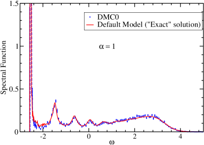
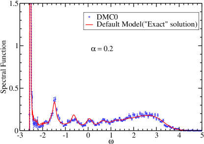
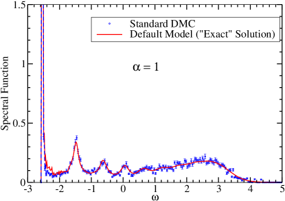
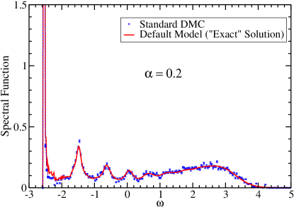
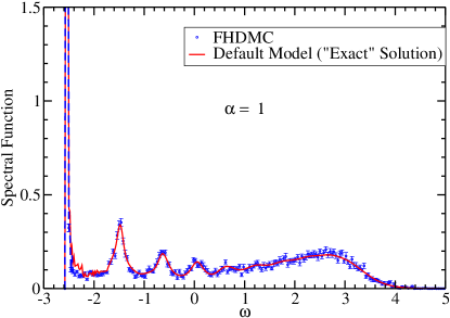
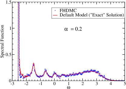
Figure 2: (Color on-line) Analytic continuation of FHDMC and standard DMC data of the $t-J$ model for $J/t=0.2$ for $\vec{k}=(\pi/2,\pi/2)$ obtained from the SAI technique using as default model the “exact” solution. Subfigures (a) and (b) are obtained using the DMC0 data for $\alpha=1$ and $\alpha=0.2$ respectively. Subfigures (c) and (d) are obtained using the standard DMC data for $\alpha=1$ and $\alpha=0.2$ respectively. Subfigures (e) and (f) are obtained using the FHDMC data for $\alpha=1$ and $\alpha=0.2$ respectively.

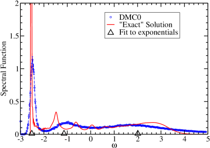
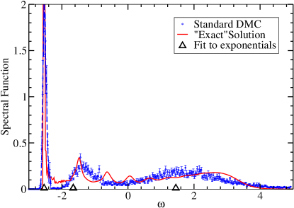
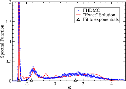
Figure 3: (Color on-line) Analytic continuation of QMC data obtained from the SAI technique using as default model a flat histogram and $\alpha=1$. Subfigure (a) is obtained using the DMC0 data. Subfigure (b) is obtained using the standard DMC data. Subfigure (c) is obtained using the FHDMC data. The black triangles pointing up show the values of the frequencies obtained by a fit to the data using three exponentials.

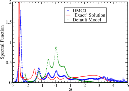
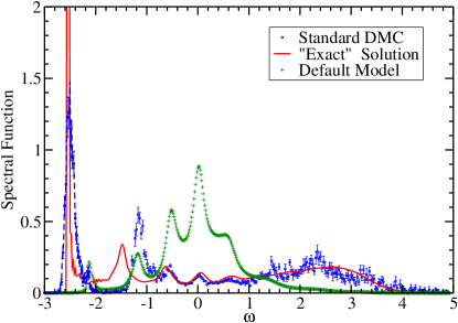
Figure 4: (Color on-line) Analytic continuation of QMC data obtained from the SAI technique using as default model the “exact” $A(k=0,\omega)$ and $\alpha=1$. Subfigure (a) is obtained using the DMC0 data. Subfigure (b) is obtained using the standard DMC data. Subfigure (c) is obtained using the FHDMC data.

IV.1 Using the “exact” as default model

In Fig. 2 we present the results of the analytic continuation of the data obtained with DMC0, the standard-DMC, and the FHDMC methods and the SAI technique, and as default model the “exact” solution (discussed in the previous section). Notice that the results using any sets of data are very close to the “exact” solution and independent of the “temperature” parameter $\alpha$ which we used. In general at higher value of $\alpha$ the role of the default model is influencing more the result of the analytic continuation.

IV.2 Using the flat distribution as default model

Since in practice an exact solution is not available to use as the default model, we wish to examine the extent to which this method can be used for the analytic continuation. Therefore, we would like to test the method when we use a default model that is different from the exact answer. Towards this goal, we have used the two different default models discussed in the previous Section. First we use the flat distribution given by Eq. 22.

Fig. 3 presents the results of the application of the SAI method using $\alpha=1$. The results for lower values of $\alpha$ are very similar. The DMC0 method yields the results illustrated in Fig. 3(a)). The standard DMC method yields the results presented in Fig. 3(b)), while the FHDMC approach yields the results illustrated in Fig. 3(c)). We least-squared fitted the DMC0, the standard-DMC, and the FHDMC data on $G(\tau)$ to the form

$$G(\tau)=Z_{1}e^{-\omega_{1}\tau}+Z_{2}e^{-\omega_{2}\tau}+Z_{3}e^{-\omega_{3}\tau},$$ (23)

and the values of the parameters $Z_{1,2,3}$ and $\omega_{1,2,3}$ found by the fit are listed in Table 1. The up-triangles in each of the subfigures show the values of the three frequencies found by the fits. Notice that the lowest two agree with the lowest two peaks found by the SAI method. In addition, the third frequency $\omega_{3}$ approximately accounts for the broad feature of the $A(\omega)$ at high frequencies with approximately the correct spectral weight which is taken into account by the value of $Z_{3}$. The value of $Z_{1}$, which corresponds to the residue of the lowest frequency quasiparticle peak, agrees rather well with the integral of $A(\omega)$ around the quasiparticle peak; thus, this agrees with the residue of the quasiparticle peak found in Ref. Liu and Manousakis (1992), which is approximately 0.2.

Method	$Z_{1}$	$Z_{2}$	$Z_{3}$	$\omega_{1}$	$\omega_{2}$	$\omega_{3}$
DMC0	0.27	0.26	0.47	-2.516	-1.14	2.01
SDMC	0.24	0.19	0.56	-2.538	-1.64	1.43
FHDMC	0.23	0.19	0.56	-2.538	-1.656	1.45

Table 1: The results of fitting the DMC0, the standard-DMC (SDMC), and the FHDMC data on $G(\tau)$ to the formula given by Eq. 23.

We notice that the results of the analytic continuation cannot reproduce the details of the exact solution even by changing the value of $\alpha$ to a significantly lower value. The overall performance of the standard DMC and the FHDMC methods are approximately the same and significantly better than the results obtained with the DMC0 method. Notice, however, that the width of the lowest energy peak is a little closer to the exact when we used the FHDMC data.

IV.3 Using $A_{(0,0)}(\omega)$ as default model

The default model used in the previous subsection assumes no a priori knowledge about the features of $A_{\vec{k}}(\omega)$. Therefore, it heavily relies on minimizing $\chi^{2}$. In many cases in practice, however, we have some partial information from either approximate analytic or semi-analytic (for example, perturbation expansion) or numerical techniques, such as from the density functional theory in electronic structure calculations. It is typical to know the approximate location of the peaks, however, it is much harder to know the spectral weight of these peaks. Next we will use the “exact” spectral function $A_{(0,0)}(\omega)$ obtained for $\vec{k}=(0,0)$ as the default model in the SAI approach to invert the DMC0, the standard-DMC, and the FHDMC data on $G_{({{\pi}\over 2},{{\pi}\over 2})}(\tau)$. As can be seen from Fig. 4, most of the peaks of the default model are close to those of the “exact” solution. The lowest energy peak is in the wrong place and the relative spectral weights (i.e., the heights of the peaks) are very different than those in the “exact” solution.

In Fig.4 we present the results of applying the SAI method to data obtained with DMC0, the standard DMC, and the FHDMC method using $\alpha=1$ and as default model the above discussed “incorrect” solution which corresponds to $\vec{k}=(0,0)$ instead of the correct value of $\vec{k}=(\pi/2,\pi/2)$. Fig.4(a) presents the results obtained using the DMC0 data. In Fig.4(b) and Fig. 4(c) we present the results of applying the SAI method to data obtained with the standard DMC and the FHDMC method respectively. The default model is shown by the green open circles. Notice that the overall performance of the standard DMC and the FHDMC methods is approximately the same and significantly better than that of the DMC0 data. Notice, however, that the width of the lowest energy quasiparticle peak when using the FHDMC data is somewhat smaller and closer to the “exact”, as compared to that obtained with the standard DMC data. Also note that the location of the second peak is closer to the “exact” location when using the FHDMC data.

These differences in the degree of approximating the low-energy features of the spectral function can be explained when we compare the relative error in $G(\tau)$ as obtained from the two methods as was done in Fig. 1(b). Fig. 1(b) compares our results for the relative error for the $G_{\vec{k}}(\tau)$ as a function of $\tau$ as obtained with the DMC0, FHDMC and standard-DMC for the approximately the same amounts of CPU time. For the case of DMC0 we have chosen $\tau_{max}=3.8$ in order to obtain a comparable error in $G(\tau)$ with the other two methods. First notice that for a fixed value of $\tau_{max}$ and for a fixed number of Monte Carlo steps in the DMC0 method, the relative error is weakly dependent of $\tau$ yielding an average value $\sigma_{r}(\tau_{max})$ for the relative error. However, for fixed number of Monte Carlo steps, this average relative error $\sigma_{r}(\tau_{max})$ in the DMC0 method grows exponentially with $\tau_{max}$. By choosing $\tau_{\max}=3.8$ we have optimized the quality of the analytic continuation. While the greater range of $\tau$ allows us to obtain better resolution for small values of $\omega$, if we increase the value of $\tau_{\max}$ beyond the above chosen value, the errors grow to the point that the quality of the analytic continuation becomes much worse. This is the reason for the superiority of the standard DMC and FHDMC methods.

We further note that the error in the standard-DMC method at short time $\tau$ is much better than the error in the FHDMC data. However, the situation reverses at long imaginary time. This helps the extraction of the low-energy physics of the problem. In the case of the present example, the crossing point of the relative error between the two methods occurs at $\tau\sim 8$, which implies that the features of the spectral function obtained with the two methods will differ for $\delta\omega/t<1/8$, (where $\delta\omega$ is measured from the lowest energy state). For the present problem this seems like a narrow range, however, in general, for other problems where we are interested in the low energy excitations it can be more important.

V Conclusions

We have shown that by combining flat histogram techniquesBerg and Newhaus (1991); Wang and Landau (2001a, b); de Oliviera et al. (1996) and the QMC method in such a way to make the histogram of an imaginary-time correlation function $G(\tau)$ flat, we are able to carry out accurate analytic continuation to real time with better degree of accuracy as compared to any quantum Monte Carlo method which does not use the flat histogram idea.

This has been demonstrated using the DMC method which can be modified to simulate an exactly soluble problem. This is within the flexibility of the DMC method, because we can select the set of Feynman diagrams to sample. Thus, by selecting the diagrammatic series to be the one which takes into account all the diagrams which contribute to the single-hole spectral function of the 2D $t-J$ model within the NCA approximation, we can compare the results of the analytic continuation directly to the “exact” solutionLiu and Manousakis (1991, 1992). To carry out the analytic continuation to real time, we have used the SAIFuchs et al. (2010) approach, a generalization of the maximum entropy method.

From this paper we draw the following main conclusions:

I) The main point of the present paper is the following. We find that if the QMC data are obtained by a technique in which the histogram of $G(\tau)$ is more or less flat, such as the FHDMC or the standard DMC, the results of the analytic continuation improve significantly as compared to the results obtained by using a QMC method (such as the DMC0 method) in which the flat histogram idea has not been applied. That is because we can approach large imaginary time with significantly small statistical error.

II) This paper provides benchmarking on the power of the FHDMC and standard DMC methods to provide data for analytic continuation to real time using an exactly soluble model. In particular comparing these two methods, we find that:

• The standard DMC method requires a value of $\mu$ in order to approximate the long-time behavior of $G(\tau)$ and this can be used to effectively make the histogram of $G(\tau)$ approximately flat. Thus, the standard DMC method requires some amount of prior work in order to determine the optimum value of $\mu$. The FHDMC method makes the histogram of $G(\tau)$ flat automatically without requiring any such a priori knowledge or prior work.

• The error on the short-time behavior of $G(\tau)$ is significantly smaller in the case of standard DMC.

• The error on the long-time behavior of $G(\tau)$ is smaller in the case of FHDMC. This allows us to obtain somewhat better quality data on the spectrum and spectral weight of the very low-energy excitations. This aspect of the FHDMC method seems to give some advantage over the standard DMC, when we are interested in the very low-energy excitations of a given system.

III) Lastly, we exploit the fact that we know the “exact” solution to this problem to draw the following additional conclusions from the present calculations:

• When we use as default model, a distribution which is close to the exact, the result of the analytic continuation is very close to the exact result.

• If the correct answer is completely unknown and we use as default model the flat distribution, the result for the location for and the residue of the lowest energy quasiparticle peak is very close to the exact value, and the location and width of the second lowest peak is also in agreement with the “exact” answer. The details of the spectral function cannot be correctly captured by the analytic continuation using a flat default model.

• If we approximately know some aspects of the solution, i.e., we use a default model which shares some features of the correct solution (such as the location of some of the peaks, but not their relative strength in the spectral function) the analytic continuation tends to correct the strength of the peaks and tends to move the incorrectly located peaks of the default model towards the correct positions.

The main point of the present paper is that, in general, if we incorporate the flat histogram idea with any QMC technique, in such a way to make the histogram of $G(\tau)$ flat, the results of the analytic continuation to real time should be of better statistical quality.

VI Acknowledgments

This work was supported in part by the U.S. National High Magnetic Field Laboratory, which is partially funded by the NSF DMR-1157490 and the State of Florida.

References

- Ceperley (1995) D. M. Ceperley, Rev. Mod. Phys. 67, 279 (1995).
- Jarrell and Gubernatis (1996) M. Jarrell and J. Gubernatis, Phys. Rep. 269, 133 (1996).
- Fuchs et al. (2010) S. Fuchs, T. Pruschke, and M. Jarrell, Phys. Rev. E 81, 056701 (2010).
- Beach (2004) K. Beach, e-print arxiv: cond-mat/ 0403055 (2004).
- Berg and Newhaus (1991) B. A. Berg and T. Newhaus, Phys. Lett. B 267, 249 (1991).
- Wang and Landau (2001a) F. Wang and D. P. Landau, Phys. Rev. Lett. 86, 2050 (2001a).
- Wang and Landau (2001b) F. Wang and D. P. Landau, Phys. Rev. E 64, 056101 (2001b).
- de Oliviera et al. (1996) P. M. C. de Oliviera et al., J. Phys. 26, 677 (1996).
- Troyer et al. (2003) M. Troyer, S. Wessel, and F. Alet, Phys. Rev. Lett. 90, 120201 (2003).
- Gull et al. (2011) E. Gull, A. J. Millis, A. I. Lichtenstein, A. N. Rubstov, M. Troyer, and P. Werner, Rev. Mod. Phys. 83, 349 (2011).
- Diamantis and Manousakis (2013) N. G. Diamantis and E. Manousakis, Phys. Rev. E 88, 043302 (2013).
- Liu and Manousakis (1991) Z. Liu and E. Manousakis, Phys. Rev. B 44, 2414 (1991).
- Liu and Manousakis (1992) Z. Liu and E. Manousakis, Phys. Rev. B 45, 2425 (1992).
- Prokof’ev and Svistunov (1998) N. V. Prokof’ev and B. V. Svistunov, Phys. Rev. Lett 81, 2514 (1998).
- Mishchenko et al. (2000) A. S. Mishchenko, N. V. Prokof’ev, A. Sakamoto, and B. V. Svistunov, Phys. Rev. B 62, 6317 (2000).
- Mishchenko et al. (2001) A. S. Mishchenko, N. V. Prokof’ev, and B. V. Svistunov, Phys. Rev. B 64, 033101 (2001).
- Mishchenko and Nagaosa (2004) A. S. Mishchenko and N. Nagaosa, Phys. Rev. Lett. 93, 036402 (2004).
- Mishchenko and Nagaosa (2006) A. S. Mishchenko and N. Nagaosa, Phys. Rev. B 73, 092502 (2006).
- Cataudella et al. (2007) V. Cataudella, G. De Filippis, A. S. Mishchenko, and N. Nagaosa, Phys. Rev. Lett. 99, 226402 (2007).
- Kane et al. (1989) C. L. Kane, P. A. Lee, and N. Read, Phys. Rev. B 39, 6880 (1989).
- Manousakis (1991) E. Manousakis, Rev. Mod. Phys. 61, 1 (1991).
- Sandvik (1998) A. W. Sandvik, Phys. Rev. B 57, 10287 (1998).
- Syljuasen (2008) O. F. Syljuasen, Phys. Rev. B 78, 174429 (2008).