Holographic renormalization and
anisotropic black branes in higher curvature gravity

Abstract

We consider five-dimensional AdS-axion-dilaton gravity with a Gauss-Bonnet term and find a solution of the equations of motion which corresponds to a black brane exhibiting a spatial anisotropy, with the source of the anisotropy being an axion field linear in one of the horizon coordinates. Our solution is static, regular everywhere on and outside the horizon, and asymptotically AdS. It is analytic and valid in a small anisotropy expansion, but fully non-perturbative in the Gauss-Bonnet coupling. We discuss various features of this solution and use it as a gravity dual to a strongly coupled anisotropic plasma with two independent central charges, $a\neq c$. In the limit of small Gauss-Bonnet coupling, we carry out holographic renormalization of the system using (a recursive variant of) the Hamilton-Jacobi method and derive a generic expression for the boundary stress tensor, which we later specialize to our solution. Finally, we compute the shear viscosity to entropy ratios and conductivities of this anisotropic plasma.

1 Introduction

The AdS/CFT correspondence Maldacena:1997re ; duality2 ; duality3 represents a remarkable tool in the study of the strongly coupled gauge theories which can be mapped to a dual, weakly coupled gravitational description. The correspondence is best understood, and mostly used, in the limit in which both $N$ and $\lambda$, the rank of the gauge group and the ’t Hooft coupling of the gauge theory, respectively, are infinite. This maps to the classical supergravity limit of the string side. Investigating departures from this limit implies introducing $\alpha^{\prime}$ and loop corrections for the string and it is clearly of the utmost importance for a series of reasons, from achieving a deeper understanding of how the correspondence works in larger regions of the parameter space, to modeling more realistic gauge theory systems, where $N$ and $\lambda$ are obviously not infinite. A systematic treatment of $\alpha^{\prime}$ and loop corrections is however a tall order, given their complexity. For example, the leading finite coupling corrections to type IIB supergravity arise as stringy corrections with schematic form $\alpha^{\prime 3}R^{4}$.

One more modest approach is to consider simple generalizations of Einstein gravity, where higher curvature corrections are under control and calculable, in the hope to gain some qualitative understanding of the effects they might have and, perhaps, uncover some universal properties. A well-studied family of corrections is represented by Lovelock theories of gravity lovelock1 ; lovelock2 ; lovelock3 ; lovelock4 . These theories are defined as natural extensions of the Einstein-Hilbert action to dimensions higher than four. The main characteristic of Lovelock gravities is the fact that, albeit being defined in terms of higher curvature/derivative terms, they yield second order equations of motion and are free of pathologies. The first Lovelock correction, which is present already in five dimensions, is given by the Gauss-Bonnet (GB) term, which is quadratic in the curvature. Another point of interest in this correction is that, besides being calculable, it possesses a wealth of exact black hole solutions with AdS asymptotics; see e.g. branches ; camanhoetal and bestiary for a comprehensive review.

It is clearly worthwhile to try to find as many new solutions as possible and increase the arena of models where explicit computations can be performed. With this motivation in mind, in this paper we consider a GB correction to Einstein-Hilbert gravity in five dimensions with a negative cosmological constant and a coupling to an axion-dilaton field. It is not clear whether this system might be obtained by some string theory compactification, so that our philosophy in this work is ‘bottom-up’.

The first result of our analysis is a new solution of the equations of motion representing a black brane with a translationally invariant but anisotropic horizon. The force responsible for keeping the horizon in an anisotropic state is furnished by the axion field, which we take to have a fixed profile in the radial coordinate but to depend linearly in one of the horizon coordinates. This is similar to what has been done in ALT and later in MT ; MT2 . This new solution is interesting from a purely General Relativity point of view, for it opens up the possibility to study the thermodynamics of a black brane which depends on several parameters (the temperature, the GB coupling and an anisotropy parameter), presumably giving rise to a rich phase space. In this paper we move a first step toward the study of such thermodynamics by computing the boundary stress tensor, which represent our second and perhaps most important result. This computation requires the machinery of holographic renormalization. More specifically, we use a Hamiltonian approach to the problem, rather than the more commonly used Lagrangian one, in the incarnation of the recursive Hamilton-Jacobi method developed in Yiannis for the AdS-Einstein system with axion-dilaton (without higher derivative corrections). Holographic renormalization of Einstein gravity with the GB term, but without any other field turned on, has been performed in LiuSabra .

A more applied motivation for our work is given by the study of the quark-gluon plasma (QGP) produced in the ultra-relativistic collision of heavy ions at RHIC rhic ; rhic2 and LHC lhc . Contrary to naïve expectations, this plasma turns out to be a strongly coupled fluid fluid ; fluid2 , rather than a quasi-ideal free gas of quarks and gluons. This fact renders a perturbative approach of limited applicability and motivates the use of the AdS/CFT correspondence; see reviewmateosetal for a review of applications of AdS/CFT to the study of the QGP. One of the diagnostics of the strongly coupled nature of this fluid is represented by ‘elliptic flow’, i.e. the anisotropic evolution of the fluid in the initial stages before isotropization. Recently, there has been some interest in modeling this anisotropy at strong coupling MT ; MT2 and in studying how various observables may be affected by it. Some of the studies that have been performed include the computation of the shear viscosity to entropy density ratio Rebhan ; mamo , the drag force experienced by a heavy quark Chernicoff:2012iq ; giataganas ; new_drag , the energy lost by a quark rotating in the transverse plane fadafan , the stopping distance of a light probe stopping , the jet quenching parameter of the medium giataganas ; Rebhan:2012bw ; jet , the potential between a quark and antiquark pair, both static giataganas ; Rebhan:2012bw ; Chernicoff:2012bu ; indians and in a plasma wind Chernicoff:2012bu , including its imaginary part Fadafan:2013bva , Langevin diffusion and Brownian motion langevin ; langevin2 ; langevin3 , chiral symmetry breaking Ali-Akbari:2013txa , the production of thermal photons photon ; Wu:2013qja ; Arciniega:2013dqa and dileptons dileptons , and the introduction of a chemical potential chempot ; chempot1 ; see Giataganas:2013lga for a review of some of these computations and seealso for similar computations in a fluid with dilaton-driven anisotropy.

In order to achieve a more realistic model of the anisotropic plasma it is obviously important to relax some of the assumptions (like the infinite coupling and infinite number of colors) that go into the simplification of having a classical gravity dual. The GB coupling that we introduce here corresponds to allowing for different central charges, $a\neq c$, in the gauge theory aneqc ; aneqc1 ; aneqc2 . We compute these two central charges for our particular solution, verifying that they are indeed different. On general grounds, looking at how higher derivative terms affect physical observables on the gauge theory might also be useful to constrain the string landscape, e.g. by excluding regions of parameters that would result in pathologies, as advocated for example in camanhoetal ; maldaedel . As a final, concrete application of our geometry we compute the shear viscosity over entropy density ratio (in a few, equivalent ways) and the plasma conductivities.

This paper is organized as follows. In Sec. 2 we present our solution and compute its temperature and entropy density. In Sec. 3 we carry out the holographic renormalization, obtaining general formulas for the expectation values of the stress tensor and of the axion and dilaton operators. In Sec. 4 we specialize those formulas to the case at hand and discuss the various features of energy density and pressures. In Sec. 5 we use the solution as a model for a strongly coupled anisotropic plasma and compute various transport coefficients of interest, such as the shear viscosity over entropy ratios, both along the anisotropic direction and in the transverse plane, using the membrane paradigm. We finally discuss our results and outline possible future extensions of our work in Sec. 6. A series of appendices contains some of the more technical details of our computations, like the explicit derivation of the solution and the derivation of the shear viscosity tensor using alternative methods.

2 Action and solution

We are interested in five-dimensional gravity with a negative cosmological constant and the inclusion of a Gauss-Bonnet term, which we also couple to an axion-dilaton system in the following way

$$S=\frac{1}{16\pi G}\int d^{5}x\,\sqrt{-g}\left[R+\frac{12}{\ell^{2}}-\frac{1}{2}(\partial\phi)^{2}-\frac{e^{2\phi}}{2}(\partial\chi)^{2}+\frac{\ell^{2}}{2}\lambda_{\textrm{\tiny GB}}{\cal L}_{\textrm{\tiny GB}}\right]+S_{\textrm{\tiny GH}}\,.$$ (1)

The scalar fields $\phi$ and $\chi$ are the dilaton and axion, respectively, $\lambda_{\textrm{\tiny GB}}$ is the (dimensionless) Gauss-Bonnet coupling and

$${\cal L}_{\textrm{\tiny GB}}=R^{2}-4R_{mn}R^{mn}+R_{mnrs}R^{mnrs}$$ (2)

is the Gauss-Bonnet term. $\ell$ is a parameter with dimensions of length that we set to one in what follows, without loss of generality. We use the Latin indices $m,n,\ldots$ for the five-dimensional coordinates $(t,x,y,z,u)$, with $u$ being the radial coordinate. The term $S_{\textrm{\tiny GH}}$ is the usual Gibbons-Hawking term, necessary to render the variational problem well posed. When $\lambda_{\textrm{\tiny GB}}=0$ the action above can be obtained from type IIB superstrings MT ; MT2 , but this is no longer true when the Gauss-Bonnet coupling is turned on. In fact, it is not clear whether (1) can be obtained from any string theory compactification, so that our point of view in the present paper is ‘bottom-up’, as already discussed in the Introduction.

The field equations for the metric resulting from the action above are given by

$$R_{mn}-\frac{1}{2}g_{mn}R+\frac{\lambda_{\textrm{\tiny GB}}}{2}\delta{{\cal L}_{\textrm{\tiny GB}}}_{mn}=\frac{1}{2}\partial_{m}\phi\,\partial_{n}\phi+\frac{1}{2}e^{2\phi}\partial_{m}\chi\,\partial_{n}\chi-\frac{g_{mn}}{4}\left[(\partial\phi)^{2}+e^{2\phi}(\partial\chi)^{2}-12\right]\,,$$ (3)

where

$$\delta{{\cal L}_{\textrm{\tiny GB}}}_{mn}=-\frac{g_{mn}}{2}{\cal L}_{\textrm{\tiny GB}}-4R_{m}^{\,\,\,\,\,r}R_{rn}+2R_{mn}R-4R^{rs}R_{mrns}+2R_{m}^{\,\,\,\,\,rst}R_{nrst}$$ (4)

is the variation of the Gauss-Bonnet term. The equations for the dilaton and axion read instead

$$\partial_{m}(\sqrt{-g}g^{mn}\partial_{n}\phi)=\sqrt{-g}e^{2\phi}(\partial\chi)^{2}\,,\qquad\partial_{m}(\sqrt{-g}e^{2\phi}g^{mn}\partial_{n}\chi)=0\,.$$ (5)

We want to obtain a solution which displays a spatial anisotropy. This is achieved by singling out one direction, say the $z$-direction, which will be later identified with the ‘beam direction’ in a heavy ion collision experiment occurring in the boundary theory. To get an anisotropy between the $z$-direction and the $xy$-directions (the transverse plane to the beam), we consider the following Ansatz

$$ds^{2}=\frac{1}{u^{2}}\left(-FB\,dt^{2}+dx^{2}+dy^{2}+H\,dz^{2}+\frac{du^{2}}{F}\right).$$ (6)

All the metric components $F$, $B$, and $H$, as well as the dilaton $\phi$, depend solely on the radial coordinate $u$. This guarantees that the solution be static. In this parametrization the boundary is located at $u=0$. $F$ is a ‘blackening factor’ that introduces an horizon in the geometry at $u=u_{\textrm{\tiny H}}$, where $F(u_{\textrm{\tiny H}})=0$. There is a scaling symmetry in the coordinates $t$ and $z$ that allows us to set $B_{\textrm{\tiny bdry}}F_{\textrm{\tiny bdry}}=H_{\textrm{\tiny bdry}}=1$, thus recovering a canonically normalized AdS metric in the UV region (with radius $1/\sqrt{F_{\textrm{\tiny bdry}}}$). Here and in what follows we use the subscript ‘bdry’ to denote the value of the fields at $u=0$.

Following ALT ; MT we consider an axion field which has a constant profile in the radial direction and depends linearly on $z$

$$\chi=a\,z\,.$$ (7)

The parameter $a$ has dimensions of energy and controls the amount of anisotropy. It is clear that this is a solution of the axion equation, since the metric is diagonal and the metric and dilaton do not depend on $z$.

In this paper we limit ourselves to considering the case of small anisotropy, which will allow for an analytic solution of the equations of motion. To do this we expand all the fields around the (isotropic) Gauss-Bonnet black brane solution

$$\phi(u) = a^{2}\phi_{2}(u)+O(a^{4})\,,$$ (8)

$$F(u) = F_{0}(u)+a^{2}F_{2}(u)+O(a^{4})\,,$$ (9)

$$B(u) = B_{0}\left(1+a^{2}B_{2}(u)+O(a^{4})\right)\,,$$ (10)

$$H(u) = 1+a^{2}H_{2}(u)+O(a^{4})\,,$$ (11)

where

$$F_{0}(u)=\dfrac{1}{2\lambda_{\textrm{\tiny GB}}}\left(1-\sqrt{1-4\lambda_{\textrm{\tiny GB}}\left(1-\frac{u^{4}}{u_{\textrm{\tiny H}}^{4}}\right)}\right)\,,\qquad\lambda_{\textrm{\tiny GB}}<\frac{1}{4}\,.$$ (12)

This is a solution of the equations of motion when $a=0$. In order to have a unit speed of light at the boundary we set

$$B_{0}=\frac{1}{2}\left(1+\sqrt{1-4\lambda_{\textrm{\tiny GB}}}\right)\,.$$ (13)

This is possible due to the scaling symmetry in $t$, which we have mentioned above. Note that only even powers of $a$ can appear in the expansion because of the symmetry $z\to-z$.

Luckily it is possible to solve the equations analytically at order $O(a^{2})$. The equations at this order and the explicit solutions are detailed in App. A. A plot of representative solutions is contained in Fig. 1, where the regularity of the geometry is explicitly exhibited.

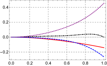
Figure 1: The metric functions at order $O(a^{2})$. Here we have set $\lambda_{\textrm{\tiny GB}}=0.2$.

Here we just mention that we have fixed the integration constants in such a way that all the metric functions are regular at the horizon and moreover

$$\phi_{2,\textrm{\tiny bdry}}=F_{2,\textrm{\tiny bdry}}=B_{2,\textrm{\tiny bdry}}=H_{2,\textrm{\tiny bdry}}=0\,,$$ (14)

thus recovering AdS in the UV. A direct computation of the Kretschmann invariant $R_{mnpq}R^{mnpq}$ shows no singularity in the geometry except for $\lambda_{\textrm{\tiny GB}}=1/4$, which is however excluded, as can be seen from (12).

Unfortunately, we have not been able to find analytic solutions beyond order $O(a^{2})$ and most likely a numerical analysis will turn out to be necessary to go to higher anisotropies. This is however beyond the scope of the present paper. It should be possible, in principle, to consider arbitrarily large values of $a$, as in the pure Einstein-Hilbert case of MT ; MT2 .

The temperature of the solution can be computed as usual from the standard requirement that the (Euclideanized) metric be regular at $u=u_{\textrm{\tiny H}}$. One finds that

$$T=-\frac{F^{\prime}(u)\sqrt{B(u)}}{4\pi}\Big{|}_{u=u_{\textrm{\tiny H}}}\,.$$ (15)

Specializing to our solution this becomes

$$T = \sqrt{B_{0}}\left(\frac{1}{\pi u_{\textrm{\tiny H}}}-\frac{2B_{0}-6\lambda_{\textrm{\tiny GB}}+\sqrt{\lambda_{\textrm{\tiny GB}}}\log\left(\frac{1+2\sqrt{\lambda_{\textrm{\tiny GB}}}}{1-2\sqrt{\lambda_{\textrm{\tiny GB}}}}\right)-\log\left(\frac{4B_{0}}{\sqrt{1-4\lambda_{\textrm{\tiny GB}}}}\right)}{48\pi(1-4\lambda_{\textrm{\tiny GB}})}u_{\textrm{\tiny H}}a^{2}+O(a^{4})\right)\,.$$ (16)

This equation can be easily inverted to find $u_{\textrm{\tiny H}}$ as a function of $T$.

For planar black holes in GB gravity the entropy density is still given by the usual formula in terms of the area of the horizon. We find (here $V_{3}$ is the infinite volume $\int dx\,dy\,dz$)

$$s=\frac{A_{\textrm{\tiny hor}}}{4GV_{3}}=\frac{\pi}{4GB_{0}^{3/2}}\left(\pi^{2}T^{3}+\frac{1}{8}TB_{0}a^{2}+O(a^{4})\right)\,.$$ (18)

We notice that for $\lambda_{\textrm{\tiny GB}}=0$ this matches the result obtained in MT ; MT2 .

A final comment on the IR behavior of the geometry is in order. The solution of MT ; MT2 was interpolating between AdS boundary conditions in the UV and a Lifshitz-like scaling solution ALT in the IR. We believe that the finite $\lambda_{\textrm{\tiny GB}}$ generalization discussed here does not share this feature with MT ; MT2 , although we have not been able to prove this rigorously. More specifically, we have not been able to find a scaling solution in the IR (even for $T=0$), as done in ALT for the case $\lambda_{\textrm{\tiny GB}}=0$. One obstruction might be that Lifshitz solutions in GB gravity seem to require to tune the cosmological constant in ways that are not compatible with our equations. For example, in the case of GB gravity coupled to a massive vector field the condition for a Lifshitz scaling is that the cosmological constant be half of the usual value Mann . It would certainly be interesting to settle this point, but this goes beyond the scope of the paper.

3 Holographic renormalization

In this section we use holographic renormalization techniques to compute the 1-point function of the boundary stress tensor associated to our gravitational system; see reviewHR for a review. In fact, we consider a generalization of (1), where the coefficient of the axion kinetic term is allowed to be a generic function $Z(\phi)$ of the dilaton. We also maintain the metric and axion-dilaton generic. We use the recursive Hamilton-Jacobi method that was introduced in Yiannis for axion-dilaton gravity without Gauss-Bonnet term. Our main result are the expressions (78)-(LABEL:chi-final) for $\langle T_{ij}\rangle$, $\langle{\cal O}_{\phi}\rangle$ and $\langle{\cal O}_{\chi}\rangle$, which are general and which we specialize to our solution (11) in the next section.

3.1 Metric and action in ADM form

The recursive Hamilton-Jacobi method of Yiannis , which we follow closely in this section, makes use of the ADM formalism, in which a manifold $\mathcal{M}$ is foliated with hypersurfaces $\Sigma_{r}$ of constant radial coordinate, which we call $r$ in this section. In this coordinate, which plays the role of Hamiltonian time, the boundary is located at $r=\infty$. The metric on $\mathcal{M}$ takes the form

$$ds^{2}=(N^{2}+N_{i}N^{i})dr^{2}+2N_{i}drdx^{i}+\gamma_{ij}dx^{i}dx^{j}\,,$$ (19)

where $N$ and $N_{i}$ are the lapse and shift function, respectively, and $\gamma_{ij}$ is the induced metric on $\Sigma_{r}$. We use the Latin indices $i,j,\ldots$ to label the coordinates $(t,x,y,z)$ on $\Sigma_{r}$. In terms of these fields, the extrinsic curvature is given by

$$K_{ij}=\frac{1}{2N}(\dot{\gamma}_{ij}-D_{i}N_{j}-D_{j}N_{i})\,,$$ (20)

with the dot denoting differentiation with respect to $r$ and $D_{i}$ being the covariant derivative associated to $\gamma_{ij}$.

The axion-dilaton part of (1), without Gauss-Bonnet contribution, turns out to be given by

$$S_{\textrm{\tiny axion-dilaton}} = \int_{\mathcal{M}}d^{d}x\sqrt{-g}\Big{[}\mathcal{R}+K^{2}-K_{ij}^{2}+(d-1)(d-2)$$ (22)

$$\hskip 71.13188pt-\frac{1}{2}\left(\dot{\phi}^{2}+Z(\phi)\dot{\chi}^{2}+\gamma^{ij}(\partial_{i}\phi\partial_{j}\phi+Z(\phi)\partial_{i}\chi\partial_{j}\chi)\right)\Big{]}\,.$$

Here and in the following we leave the function in the axion kinetic term as a generic function of the dilaton, $Z(\phi)$. Later we will specialize to $Z(\phi)=e^{2\phi}$ and to $d=5$, which is the case considered in the previous section. We denote with the calligraphic fonts $\mathcal{R}$, $\mathcal{R}_{ij}$, etc. the curvature on $\cal{M}$ computed in terms of $N,N_{i}$ and $\gamma_{ij}$. All the contractions of the $i,j,\ldots$ indices are performed with $\gamma^{ij}$. The Gauss-Bonnet contribution is (see for example eq. (2.8) of LiuSabra )

$$S_{\textrm{\tiny GB}} = \frac{1}{2}\int_{\mathcal{M}}d^{d}x\sqrt{-g}\left[(\mathcal{R}^{2}+K^{2}-K_{ij}^{2})^{2}-4(\mathcal{R}_{ij}+KK_{ij}-K_{ik}K_{j}^{k})^{2}\right.$$ (23)

$$\hskip 85.35826pt+(\mathcal{R}_{ijkl}+K_{ik}K_{jl}-K_{il}K_{jk})^{2}-\frac{4}{3}K^{4}+8K^{2}K_{ij}^{2}$$

$$\hskip 113.81102pt\left.-\frac{32}{3}KK_{i}^{j}K_{j}^{k}K_{k}^{i}-4(K_{ij}^{2})^{2}+8K_{i}^{j}K_{j}^{k}K_{k}^{l}K_{l}^{i}\right]\,,$$

with $K=\gamma^{ij}K_{ij}$. The Gibbons-Hawking terms have already been included in the actions above, but they get canceled by boundary terms coming from the bulk actions. The total action is then

$$S=S_{\textrm{\tiny axion-dilaton}}+\lambda_{\textrm{\tiny GB}}S_{\textrm{\tiny GB}}\,.$$ (24)

3.2 Radial evolution Hamiltonian

The next ingredient in the algorithm is to compute the Hamiltonian for radial evolution, which is associated to the Lagrangian $L$ defined by $S=\int drL$. To this scope, we need the canonical conjugate momenta

$$\pi^{ij} \equiv \frac{1}{\sqrt{-\gamma}}\frac{\delta L}{\delta\dot{\gamma}_{ij}}$$

$$= \gamma^{ij}K-K^{ij}\ +\lambda_{\textrm{\tiny GB}}\left[\gamma^{ij}(\mathcal{R}K-2\mathcal{R}_{kl}K^{kl})-\mathcal{R}K^{ij}-2\mathcal{R}^{ij}K+4\mathcal{R}^{k(i}K^{j)}_{\;k}\right.$$

$$\hskip 113.81102pt+2\mathcal{R}^{ikjl}K_{kl}+\frac{1}{3}\gamma^{ij}(-K^{3}+3KK_{kl}^{2}-2K_{k}^{l}K_{l}^{m}K_{m}^{k})$$

$$\hskip 142.26378pt\left.+K^{2}K^{ij}-2KK_{k}^{i}K^{jk}-K^{ij}K_{kl}^{2}+2K_{k}^{i}K_{l}^{k}K^{jl}\right],$$

$$\pi_{\phi} \equiv \frac{1}{\sqrt{-\gamma}}\frac{\delta L}{\delta\dot{\phi}}=-\dot{\phi},\qquad\pi_{\chi}\equiv\frac{1}{\sqrt{-\gamma}}\frac{\delta L}{\delta\dot{\chi}}=-Z(\phi)\dot{\chi}\,.$$ (26)

In our solution it is clear that $\pi_{\chi}=0$, but we keep this term in this section for full generality. The Hamiltonian for radial evolution is then given by

$$H=\int_{\Sigma_{r}}d^{d-1}x\sqrt{-\gamma}(2\pi^{ij}K_{ij}+\pi_{\phi}\dot{\phi}+\pi_{\chi}\dot{\chi})-L\,,$$ (27)

where we used that $K_{ij}=\dot{\gamma}_{ij}/2$ in the chosen gauge. To write the Hamiltonian in terms of the canonical momenta and induced metric one needs to invert (3.2), which is a complicated system of nonlinear equations. This has been done in LiuSabra , but only to first order in $\lambda_{\textrm{\tiny GB}}$. In this section we also limit ourselves to this regime, for simplicity (although, we repeat, our solution (11) is fully non-perturbative in $\lambda_{\textrm{\tiny GB}}$). Using the results from that paper and adding the axion-dilaton contribution, we find that

$$H = -\int_{\Sigma_{r}}d^{d-1}x\sqrt{-\gamma}\Bigl{[}\mathcal{R}+(d-1)(d-2)-\frac{1}{d-2}(\pi_{i}^{i})^{2}+\pi_{ij}^{2}+\pi_{\phi}^{2}+\frac{\pi_{\chi}^{2}}{Z(\phi)}$$ (28)

$$\hskip 42.67912pt-\frac{1}{2}\bigl{(}(\partial_{i}\phi)^{2}+Z(\phi)(\partial_{i}\chi)^{2}\bigr{)}+\frac{\lambda_{\textrm{\tiny GB}}}{2}\Bigl{(}\mathcal{R}^{2}-4\mathcal{R}_{ij}^{2}+\mathcal{R}_{ijkl}^{2}-\frac{16}{d-2}\pi_{k}^{k}\mathcal{R}_{ij}\pi^{ij}$$

$$\hskip 42.67912pt+\frac{2d}{(d-2)^{2}}(\pi_{i}^{i})^{2}\mathcal{R}-2\mathcal{R}\pi_{ij}^{2}+8\mathcal{R}_{ij}\pi^{jk}\pi^{i}_{k}+4\mathcal{R}_{ijkl}\pi^{ik}\pi^{jl}+2\pi^{j}_{i}\pi^{k}_{j}\pi^{l}_{k}\pi^{i}_{l}-(\pi_{ij}^{2})^{2}$$

$$\hskip 42.67912pt-\frac{16}{3(d-2)}\pi^{l}_{l}\pi_{i}^{j}\pi_{j}^{k}\pi_{k}^{i}+\frac{2d}{(d-2)^{2}}(\pi_{k}^{k})^{2}\pi_{ij}^{2}-\frac{3d-4}{3(d-2)^{3}}(\pi_{i}^{i})^{4}\Bigr{)}\Bigr{]}+O(\lambda_{\textrm{\tiny GB}}^{2})\,.$$

More details about the derivation of this result are reported in App. B.

3.3 Recursive method

Consider now a regularized space $\mathcal{M}_{r}$, whose boundary is $\Sigma_{r}$, with a fixed $r$ which in the end is meant to be taken to infinity. We add a generic boundary term $S_{b}$ to the action defined on this regularized space. In Yiannis it was shown that the variational problem is well defined if

$$S_{b}\big{|}_{r}=-\mathcal{S}_{r},$$ (29)

where $\mathcal{S}_{r}$ is Hamilton’s principal functional, given by the on-shell action with arbitrary boundary values for $\gamma_{ij},\phi$, and $\chi$ on $\Sigma_{r}$.

It is well known that the canonical momenta can be obtained by taking functional derivatives of ${\cal S}_{r}$

$$\pi^{ij}=\frac{\delta\mathcal{S}_{r}}{\delta\gamma_{ij}},\qquad\pi_{\phi}=\frac{\delta\mathcal{S}_{r}}{\delta\phi},\qquad\pi_{\chi}=\frac{\delta\mathcal{S}_{r}}{\delta\chi}.$$ (30)

The Hamiltonian is constrained to vanish as a result of the equations of motion for $N$ and $N_{i}$

$$H=0\,.$$ (31)

We can determine $\mathcal{S}_{r}$ by solving this constraint. The trick is to consider an expansion in eigenfunctions of the operator

$$\delta_{\gamma}=\int_{\Sigma_{r}}d^{d-1}x\,2\gamma_{ij}\frac{\delta}{\delta\gamma_{ij}}.$$ (32)

One can verify that such an expansion is a derivative expansion

$$\mathcal{S}_{r}=\mathcal{S}_{(0)}+\mathcal{S}_{(2)}+\mathcal{S}_{(4)}+\ldots\,,$$ (33)

with

$$\delta_{\gamma}\mathcal{S}_{(2n)}=(d-1-2n)\mathcal{S}_{(2n)}\,.$$ (34)

Once we know the solution for $\mathcal{S}_{(0)}$, we can compute corrections to the action in a systematic way by solving algebraic equations. In fact, having to deal with algebraic equations instead of partial differential equations is the main advantage of the method of Yiannis .

Now we write Hamilton’s principal functional as

$$\mathcal{S}_{r}=\int_{\Sigma_{r}}d^{d-1}x\,\left(\mathcal{L}_{(0)}+\mathcal{L}_{(2)}+\mathcal{L}_{(4)}+\ldots\right)\,.$$ (35)

From (30) we see that the canonical momenta also admit derivative expansions

$$\pi^{ij} ={{\pi_{(0)}}}^{ij}+{{\pi_{(2)}}}^{ij}+{\pi_{(4)}}^{ij}+\ldots\,,$$ (36)

$$\pi_{\phi} ={\pi_{\phi}}_{(0)}+{\pi_{\phi}}_{(2)}+{\pi_{\phi}}_{(4)}+\ldots\,,$$ (37)

$$\pi_{\chi} ={\pi_{\chi}}_{(0)}+{\pi_{\chi}}_{(2)}+{\pi_{\chi}}_{(4)}+\ldots\,.$$ (38)

Translating (34) in terms of the momenta and the Lagrangian density we obtain

$$2\pi_{(2n)}=\frac{1}{\sqrt{-\gamma}}(d-1-2n)\mathcal{L}_{(2n)}\,,$$ (39)

where $\pi_{(2n)}={\pi_{(2n)}}^{i}_{\;i}$ is the trace taken with respect to $\gamma^{ij}$. This relation is crucial for the algorithm to work. Note that we can obtain all canonical momenta at some given order by just knowing the trace of the momentum conjugate to the induced metric.

We can now solve the Hamiltonian constraint $H=0$. Substituting the above expansions in the Hamiltonian and grouping terms with the same number of derivatives leads to an equation of the form

$$H=H_{(0)}+H_{(2)}+H_{(4)}+\ldots=0\,,$$ (40)

which must be satisfied order by order, imposing separately $H_{(2n)}=0$ for all $n$.

3.3.1 Solution at zeroth order

We start by collecting terms with zero derivatives, which results in

$$H_{(0)} = -(d-2)(d-1)-{\pi^{2}_{(0)}}_{ij}+\frac{\pi_{(0)}^{2}}{d-2}-{\pi^{2}_{\phi}}_{(0)}-\frac{{\pi^{2}_{\chi}}_{(0)}}{Z(\phi)}$$ (43)

$$+\lambda_{\textrm{\tiny GB}}\left(\frac{1}{2}({\pi^{2}_{(0)}}_{ij})^{2}-\frac{d\,{\pi^{2}_{(0)}}_{ij}\pi_{(0)}^{2}}{(d-2)^{2}}+\frac{(3d-4)\pi_{(0)}^{4}}{6(d-2)^{3}}-{\pi_{(0)}}_{i}^{k}\pi_{(0)}^{ij}\left({\pi_{(0)}}_{j}^{l}{\pi_{(0)}}_{kl}+\frac{8{\pi_{(0)}}_{jk}\pi_{(0)}}{6-3d}\right)\right)$$

$$+O(\lambda_{\textrm{\tiny GB}}^{2})\,.$$

Following Yiannis , we try with the Ansatz for $\mathcal{L}_{(0)}$

$$\mathcal{S}_{(0)}=2\int_{\Sigma_{r}}d^{d-1}x\sqrt{-\gamma}\,{\cal W}(\phi,\chi)\,,$$ (44)

and compute the corresponding canonical momenta

$$\pi_{(0)}^{ij}=\frac{\delta{\cal S}_{(0)}}{\delta\gamma_{ij}}=\gamma^{ij}{\cal W}\,,\qquad{\pi_{\phi}}_{(0)}=\frac{\delta{\cal S}_{(0)}}{\delta\phi}=2\partial_{\phi}{\cal W}\,,\qquad{\pi_{\chi}}_{(0)}=\frac{\delta{\cal S}_{(0)}}{\delta\chi}=2\partial_{\chi}{\cal W}\,.$$ (45)

Substituting into $H_{(0)}$ this gives

$$H_{(0)} = -(d-2)(d-1)+\frac{(d-1){\cal W}^{2}}{d-2}-\frac{4(\partial_{\chi}{\cal W})^{2}}{Z(\phi)}-4(\partial_{\phi}{\cal W})^{2}$$ (47)

$$\hskip 85.35826pt+\lambda_{\textrm{\tiny GB}}\left(\frac{(d-4)(d-3)(d-1){\cal W}^{4}}{6(d-2)^{3}}\right)+O(\lambda_{\textrm{\tiny GB}}^{2})\,.$$

We know from Yiannis that in the limit $\lambda_{\textrm{\tiny GB}}\to 0$ the solution for ${\cal W}$ is the constant $d-2$. We can then write

$${\cal W}(\phi,\chi)=(d-2)+\lambda_{\textrm{\tiny GB}}{\cal V}(\phi,\chi)+O(\lambda_{\textrm{\tiny GB}}^{2}).$$ (48)

Plugging (48) into (47) gives an equation for ${\cal V}(\phi,\chi)$, whose solution turns out to be also a constant

$${\cal V}=-\frac{1}{12}(d-4)(d-3)(d-2).$$ (49)

3.3.2 Solution at second order

Terms with two derivatives can be collected into the following expression

$$H_{(2)} = -{\cal R}-2\pi_{(0)}^{ij}{\pi_{(2)}}_{ij}+\frac{2\pi_{(0)}\pi_{(2)}}{d-2}-2{\pi_{\phi}}_{(0)}{\pi_{\phi}}_{(2)}-\frac{2{\pi_{\chi}}_{(0)}{\pi_{\chi}}_{(2)}}{Z(\phi)}+\frac{1}{2}(\partial_{i}\phi)^{2}+\frac{1}{2}Z(\phi)(\partial_{i}\chi)^{2}$$ (50)

$$-\lambda_{\textrm{\tiny GB}}\left[4{\cal R}^{ij}{\pi_{(0)}}_{i}^{k}{\pi_{(0)}}_{jk}+2{\cal R}_{ikjl}\pi_{(0)}^{ij}\pi_{(0)}^{kl}+\frac{d\,{\cal R}\pi_{(0)}^{2}}{(d-2)^{2}}+\frac{2d\,\pi_{(0)}^{ij}\pi_{(0)}^{2}{\pi_{(2)}}_{ij}}{\bigl{(}d-2\bigr{)}^{2}}\right.$$

$$-\frac{8{\pi_{(0)}}_{i}^{k}\pi_{(0)}^{ij}\pi_{(0)}{\pi_{(2)}}_{jk}}{d-2}+4{\pi_{(0)}}_{i}^{k}\pi_{(0)}^{ij}{\pi_{(0)}}_{j}^{l}{\pi_{(2)}}_{kl}+\frac{8{\pi_{(0)}}_{i}^{k}\pi_{(0)}^{ij}{\pi_{(0)}}_{jk}\pi_{(2)}}{6-3d}+\frac{8\pi_{(0)}^{3}\pi_{(2)}}{3\bigl{(}d-2\bigr{)}^{3}}$$

$$\left.-\frac{2d\,\pi_{(0)}^{3}\pi_{(2)}}{\bigl{(}d-2\bigr{)}^{3}}-{\pi_{(0)}}_{ij}\left(\frac{8{\cal R}^{ij}\pi_{(0)}}{d-2}+\pi_{(0)}^{ij}\left({\cal R}+2\pi_{(0)}^{kl}{\pi_{(2)}}_{kl}-\frac{2d\,\pi_{(0)}\pi_{(2)}}{(d-2)^{2}}\right)\right)\right]+O(\lambda_{\textrm{\tiny GB}}^{2})\,.$$

Substitution of the zeroth order solution in $H_{(2)}$ leads to the following simple algebraic equation for $\pi_{(2)}$

$$\left(-2+(1+(d-4)(d-3)\lambda_{\textrm{\tiny GB}}){\cal R}-\frac{1}{2}(d-4)(d-3)\lambda_{\textrm{\tiny GB}}\right)\pi_{(2)}-\frac{1}{2}(\partial_{i}\phi)^{2}-\frac{1}{2}Z(\phi)(\partial_{i}\chi)^{2}=0\,.$$ (52)

Solving the above equation and using (39), we obtain $\mathcal{L}_{(2)}$

$$\mathcal{L}_{(2)} = \frac{\sqrt{-\gamma}}{2(d-3)}\left(2{\cal R}-(\partial_{i}\phi)^{2}-Z(\phi)(\partial_{i}\chi)^{2}+\lambda_{\textrm{\tiny GB}}\frac{12-7d+d^{2}}{4}\left(6{\cal R}+(\partial_{i}\phi)^{2}+Z(\phi)(\partial_{i}\chi)^{2}\right)\right)$$ (54)

$$+O(\lambda_{\textrm{\tiny GB}}^{2})\,.$$

From this we can compute the momenta at second order

$$\pi_{(2)}^{ij} = -\frac{1}{8(d-3)}\Bigl{[}4(2{\cal R}^{ij}-\partial^{i}\phi\partial^{j}\phi-Z(\phi)\partial^{i}\chi\partial^{j}\chi)-2\gamma^{ij}(2{\cal R}-(\partial_{k}\phi)^{2}-Z(\phi)(\partial_{k}\chi)^{2})$$

$$+\lambda_{\textrm{\tiny GB}}(12-7d+d^{2})\left(6{\cal R}^{ij}+\partial^{i}\phi\partial^{j}\phi+Z(\phi)\partial^{i}\chi\partial^{j}\chi-\tfrac{1}{2}\gamma^{ij}(6{\cal R}+(\partial_{k}\phi)^{2}+Z(\phi)(\partial_{k}\chi)^{2})\right)\Bigr{]}$$

$$+O(\lambda_{\textrm{\tiny GB}}^{2})\,,$$

$${\pi_{\phi}}_{(2)} = \frac{2-\tfrac{1}{2}(12-7d+d^{2})\lambda_{\textrm{\tiny GB}}}{4(d-3)}\left(2D_{i}D^{i}\phi-Z^{\prime}(\phi)(\partial_{i}\chi)^{2}\right)+O(\lambda_{\textrm{\tiny GB}}^{2})\,,$$

$${\pi_{\chi}}_{(2)} = \frac{2-\tfrac{1}{2}(12-7d+d^{2})\lambda_{\textrm{\tiny GB}}}{2(d-3)}\left(Z(\phi)D_{i}D^{i}\chi+Z^{\prime}(\phi)\partial_{i}\chi\partial^{i}\phi\right)+O(\lambda_{\textrm{\tiny GB}}^{2})\,.$$ (56)

3.3.3 Solution at fourth order

Finally, at fourth order we have

$$H_{(4)} =-{\pi_{(2)}}_{ij}\pi_{(2)}^{ij}+\frac{\pi_{(2)}^{2}}{d-2}-{\pi^{2}_{\phi}}_{(2)}-\frac{{\pi^{2}_{\chi}}_{(2)}}{Z(\phi)}-2\pi_{(0)}^{ij}{\pi_{(4)}}_{ij}+\frac{2\pi_{(0)}\pi_{(4)}}{d-2}-2{\pi_{\phi}}_{(0)}{\pi_{\phi}}_{(4)}-\frac{2{\pi_{\chi}}_{(0)}{\pi_{\chi}}_{(4)}}{Z(\phi)}$$ (57)

$$-\lambda_{\textrm{\tiny GB}}\left[-2{\cal R}_{ij}{\cal R}^{ij}+\tfrac{1}{2}{\cal R}^{2}+\tfrac{1}{2}({\cal R}_{ijkl})^{2}-2{\cal R}\pi_{(0)}^{ij}{\pi_{(2)}}_{ij}-\frac{8{\cal R}^{ij}\pi_{(0)}{\pi_{(2)}}_{ij}}{d-2}+8{\cal R}^{ij}{\pi_{(0)}}_{i}{}^{k}{\pi_{(2)}}_{jk}\right.$$

$$+\frac{d\pi_{(0)}^{2}{\pi_{(2)}}_{ij}\pi_{(2)}^{ij}}{(d-2)^{2}}-\frac{8\pi_{(0)}^{ij}\pi_{(0)}{\pi_{(2)}}_{i}{}^{k}{\pi_{(2)}}_{jk}}{d-2}+2\pi_{(0)}^{ij}\pi_{(0)}^{kl}{\pi_{(2)}}_{ik}{\pi_{(2)}}_{jl}-2\pi_{(0)}^{ij}\pi_{(0)}^{kl}{\pi_{(2)}}_{ij}{\pi_{(2)}}_{kl}$$

$$+4{\pi_{(0)}}_{i}{}^{k}\pi_{(0)}^{ij}{\pi_{(2)}}_{j}{}^{l}{\pi_{(2)}}_{kl}+4{\cal R}_{ikjl}\pi_{(0)}^{ij}\pi_{(2)}^{kl}-{\pi_{(0)}}_{ij}\pi_{(0)}^{ij}{\pi_{(2)}}_{kl}\pi_{(2)}^{kl}-\frac{8{\cal R}^{ij}{\pi_{(0)}}_{ij}\pi_{(2)}}{d-2}+\frac{2d{\cal R}\pi_{(0)}\pi_{(2)}}{(d-2)^{2}}$$

$$+\frac{4d\pi_{(0)}^{ij}\pi_{(0)}{\pi_{(2)}}_{ij}\pi_{(2)}}{(d-2)^{2}}-\frac{8{\pi_{(0)}}_{i}{}^{k}\pi_{(0)}^{ij}{\pi_{(2)}}_{jk}\pi_{(2)}}{d-2}+\frac{d{\pi_{(0)}}_{ij}\pi_{(0)}^{ij}\pi_{(2)}^{2}}{(d-2)^{2}}+\frac{4\pi_{(0)}^{2}\pi_{(2)}^{2}}{(d-2)^{3}}-\frac{3d\pi_{(0)}^{2}\pi_{(2)}^{2}}{(d-2)^{3}}$$

$$+\frac{2d\pi_{(0)}^{ij}\pi_{(0)}^{2}{\pi_{(4)}}_{ij}}{(d-2)^{2}}-\frac{8{\pi_{(0)}}_{i}^{k}\pi_{(0)}^{ij}\pi_{(0)}{\pi_{(4)}}_{jk}}{d-2}+4{\pi_{(0)}}_{i}^{k}\pi_{(0)}^{ij}{\pi_{(0)}}_{j}^{l}{\pi_{(4)}}_{kl}-2{\pi_{(0)}}_{ij}\pi_{(0)}^{ij}\pi_{(0)}^{kl}{\pi_{(4)}}_{kl}$$

$$\left.+\frac{8{\pi_{(0)}}_{i}^{k}\pi_{(0)}^{ij}{\pi_{(0)}}_{jk}\pi_{(4)}}{6-3d}+\frac{2d{\pi_{(0)}}_{ij}\pi_{(0)}^{ij}\pi_{(0)}\pi_{(4)}}{(d-2)^{2}}+\frac{8\pi_{(0)}^{3}\pi_{(4)}}{3(d-2)^{3}}-\frac{2d\pi_{(0)}^{3}\pi_{(4)}}{(d-2)^{3}}\right]+O(\lambda_{\textrm{\tiny GB}}^{2})\,.$$ (58)

Now we repeat the previous steps. We substitute the zeroth and second order solutions in $H_{(4)}$, which leads to an algebraic equation for $\pi_{(4)}$ that can be readily solved. There is a subtlety due to the fact that the relation (39) is ill defined for $d=5$, which is our case of interest. In fact

$$\mathcal{L}_{(4)}=\sqrt{-\gamma}\frac{2}{d-5}\pi_{(4)}.$$ (59)

However, the Hamilton-Jacobi method can still be applied (see the discussion in Yiannis ) if we set the radial cut-off to be

$$r=\frac{1}{d-5}\,,$$ (60)

and define $\tilde{\mathcal{L}}_{(4)}$ such that $\mathcal{L}_{(4)}|_{r}=-2r\tilde{\mathcal{L}}_{(4)}|_{r}$, namely $\tilde{\mathcal{L}}_{(4)}=-\sqrt{-\gamma}\pi_{(4)}$. Proceeding in this way we finally arrive at

$$\frac{96}{r\sqrt{-\gamma}}\mathcal{L}_{(4)} =-8{\cal R}\left({\cal R}-(\partial_{i}\phi)^{2}-Z(\phi)\partial_{i}\chi\partial^{i}\chi\right)+4(\partial_{i}\phi)^{4}+12Z(\phi)(\partial_{i}\chi\partial^{i}\phi)^{2}$$

$$-4Z(\phi)(\partial_{i}\phi)^{2}(\partial_{j}\chi)^{2}+4Z(\phi)^{2}(\partial_{i}\chi)^{4}+24{\cal R}_{ij}\left({\cal R}^{ij}-\partial^{i}\phi\partial^{j}\phi-Z(\phi)\partial^{i}\chi\partial^{j}\chi\right)$$

$$+24\left(D_{i}D^{i}\phi-\tfrac{Z^{\prime}(\phi)}{2}(\partial_{i}\chi)^{2}\right)^{2}+24Z(\phi)\left(D_{i}D^{i}\chi+\tfrac{Z^{\prime}(\phi)}{Z(\phi)}(\partial_{i}\chi\partial^{i}\phi)\right)^{2}$$

$$+\lambda_{\textrm{\tiny GB}}\Big{[}76{\cal R}^{2}+48{\cal R}_{ijkl}{\cal R}^{ijkl}-12{\cal R}\left((\partial_{i}\phi)^{2}+Z(\phi)(\partial_{i}\chi)^{2}\right)+2(\partial_{i}\phi)^{4}+6Z(\phi)(\partial_{i}\chi\partial^{i}\phi)^{2}$$

$$-2Z(\phi)(\partial_{i}\phi)^{2}(\partial_{j}\chi)^{2}+2Z(\phi)^{2}(\partial_{i}\chi)^{4}-12{\cal R}_{ij}\left(23{\cal R}^{ij}-3\partial^{i}\phi\partial^{j}\phi-3Z(\phi)\partial^{i}\chi\partial^{j}\chi\right)$$

$$\left.-36\left(D_{i}D^{i}\phi-\tfrac{Z^{\prime}(\phi)}{2}(\partial_{i}\chi)^{2}\right)^{2}-36Z(\phi)\left(D_{i}D^{i}\chi+\tfrac{Z^{\prime}(\phi)}{Z(\phi)}\partial_{i}\chi\partial^{i}\phi\right)^{2}\right]+O(\lambda_{\textrm{\tiny GB}}^{2})\,.$$ (61)

Up to some overall factor, this expression coincides with the conformal anomaly, as we shall see in a moment.

3.4 Fefferman-Graham expansions

From the counterterms obtained using the Hamilton-Jacobi method we see that the canonical momenta take the form

$$\pi^{ij} =\pi_{(0)}^{ij}+\pi_{(2)}^{ij}-2r{}\tilde{\pi}_{(4)}^{ij}+\pi_{(4)}^{ij}+\ldots\,,$$ (62)

$$\pi_{\phi} ={\pi_{\phi}}_{(0)}+{\pi_{\phi}}_{(2)}-2r{{}\tilde{\pi}_{\phi}}_{(4)}+{\pi_{\phi}}_{(4)}+\ldots\,,$$ (63)

$$\pi_{\chi} ={\pi_{\chi}}_{(0)}+{\pi_{\chi}}_{(2)}-2r{{}\tilde{\pi}_{\chi}}_{(4)}+{\pi_{\chi}}_{(4)}+\ldots\,.$$ (64)

The fourth order terms $\pi_{(4)}^{ij},{\pi_{\phi}}_{(4)},{\pi_{\chi}}_{(4)}$ contain the information about the renormalized one-point functions. In order to determine these terms, we proceed with the asymptotic analysis. In Fefferman-Graham (FG) coordinates, the metric reads

$$ds^{2}=\ell_{AdS}^{2}\left(\frac{dv^{2}}{v^{2}}+\gamma_{ij}(x,v)\,dx^{i}dx^{j}\right)\,.$$ (65)

As already mentioned in Sec. 2, the AdS radius $\ell_{AdS}$ is given by

$$\ell_{AdS}=\frac{1}{\sqrt{F_{\textrm{\tiny bdry}}}}\,,$$ (66)

and $v=e^{-r/\ell_{AdS}}$. Generically, the fields will have the following near-boundary expansions in these coordinates

$$\gamma_{ij} =\frac{1}{v^{2}}\Big{(}g_{(0)ij}+v^{2}g_{(2)ij}+v^{4}\left(g_{(4)ij}+2h_{(4)ij}\log v\right)+O(v^{6})\Big{)}\,,$$ (67)

$$\phi =\phi_{(0)}+v^{2}\phi_{(2)}+v^{4}\left(\phi_{(4)}+2\,\tilde{\phi}_{(4)}\log v\right)+O(v^{6})\,,$$ (68)

$$\chi =\chi_{(0)}+v^{2}\chi_{(2)}+v^{4}\left(\chi_{(4)}+2\,\tilde{\chi}_{(4)}\log v\right)+O(v^{6})\,.$$ (69)

The coefficients ${g_{(0)}}_{ij},\phi_{(0)}$ and $\chi_{(0)}$ remain undetermined from this analysis, but the other coefficients can be obtained as functions of ${g_{(0)}}_{ij},\phi_{(0)}$ and $\chi_{(0)}$ by substituting the above expansions in (3.2) and comparing order by order in $v$. For example, comparing terms at order $O(v^{2})$ we obtain

$${g_{(2)}}_{ij} = -\frac{1-\lambda_{\textrm{\tiny GB}}}{2}R_{ij}+\frac{1}{4}(1+\lambda_{\textrm{\tiny GB}})\left(\partial_{i}\phi_{(0)}\partial_{j}\phi_{(0)}+Z(\phi_{(0)})\partial_{i}\chi_{(0)}\partial_{j}\chi_{(0)}\right)$$ (72)

$$+\frac{1}{24}{g_{(0)}}_{ij}\left(2(1-\lambda_{\textrm{\tiny GB}})R-(1+\lambda_{\textrm{\tiny GB}})(\partial_{k}\phi_{(0)}\partial^{k}\phi_{(0)}+Z(\phi_{(0)})\partial_{k}\chi_{(0)}\partial^{k}\chi_{(0)})\right)$$

$$+O(\lambda_{\textrm{\tiny GB}}^{2})\,,$$

$$\phi_{(2)} = \frac{1-\lambda_{\textrm{\tiny GB}}}{8}\left(2D_{(0)i}\partial^{i}\phi_{(0)}-Z^{\prime}(\phi_{(0)})\partial_{i}\chi_{(0)}\partial^{i}\chi_{(0)}\right)+O(\lambda_{\textrm{\tiny GB}}^{2})\,,$$ (73)

$$\chi_{(2)} = \frac{1-\lambda_{\textrm{\tiny GB}}}{4Z(\phi_{(0)})}\left(Z(\phi_{(0)})D_{(0)i}\partial^{i}\chi_{(0)}+Z^{\prime}(\phi_{(0)})\partial_{i}\chi_{(0)}\partial^{i}\phi_{(0)}\right)+O(\lambda_{\textrm{\tiny GB}}^{2})\,.$$ (74)

Here and in the following the curvatures $R$ and $R_{ij}$ are the ones for $g_{(0)ij}$. Comparing the logarithmic term, we obtain instead

$$\tilde{\pi}_{(4)ij} = 2\left(1-\lambda_{\textrm{\tiny GB}}\right)\left({h_{(4)}}_{ij}-{h_{(4)}}^{k}{}_{k}{g_{(0)}}_{ij}\right)+O(\lambda_{\textrm{\tiny GB}}^{2})\,,$$ (75)

$$\tilde{\phi}_{(4)} = \frac{1}{4}(1-\lambda_{\textrm{\tiny GB}}){\tilde{\pi}}_{\phi(4)}+O(\lambda_{\textrm{\tiny GB}}^{2})\,,\qquad\tilde{\chi}_{(4)}=\frac{1-\lambda_{\textrm{\tiny GB}}}{4Z(\phi_{(0)})}{\tilde{\pi}}_{\chi(4)}+O(\lambda_{\textrm{\tiny GB}}^{2})\,.$$ (76)

3.5 The 1-point functions

The order $O(v^{4})$ leads to the following renormalized one-point functions, which represent the main result of our analysis in this section. For the stress tensor we get

$$\langle T_{ij}\rangle = 2{\pi_{(4)}}_{ij}$$ (78)

$$= -2{g_{(2)}}_{ij}{g_{(2)}}^{k}{}_{k}+4{g_{(4)}}_{ij}+2{h_{(4)}}_{ij}+2{g_{(2)}}_{kl}{g_{(2)}}^{kl}{g_{(0)}}_{ij}-4{g_{(4)}}^{k}{}_{k}{g_{(0)}}_{ij}-2{h_{(4)}}^{k}{}_{k}{g_{(0)}}_{ij}$$

$$+\tfrac{1}{2}{g_{(2)}}^{kl}{g_{(0)}}_{ij}R_{kl}-\tfrac{1}{2}{g_{(2)}}_{ij}R-\tfrac{1}{2}{D_{(0)}}_{i}\phi_{(2)}{D_{(0)}}_{j}\phi_{(0)}-\tfrac{1}{2}{D_{(0)}}_{i}\phi_{(0)}{D_{(0)}}_{j}\phi_{(2)}$$

$$-\tfrac{Z(\phi_{(0)})}{2}{D_{(0)}}_{i}\chi_{(2)}{D_{(0)}}_{j}\chi_{(0)}+\tfrac{Z(\phi_{(0)})}{2}{g_{(0)}}_{ij}{D_{(0)}}_{k}\chi_{(2)}{D_{(0)}}^{k}\chi_{(0)}$$

$$-\tfrac{Z(\phi_{(0)})}{2}{D_{(0)}}_{i}\chi_{(0)}{D_{(0)}}_{j}\chi_{(2)}-\tfrac{1}{2}{D_{(0)}}_{j}{D_{(0)}}_{i}{g_{(2)}}^{k}{}_{k}+\tfrac{1}{2}{D_{(0)}}_{k}{D_{(0)}}_{i}{g_{(2)}}_{j}{}^{k}$$

$$+\tfrac{1}{2}{D_{(0)}}_{k}{D_{(0)}}_{j}{g_{(2)}}_{i}{}^{k}-\tfrac{1}{2}D_{(0)k}D^{k}_{(0)}{g_{(2)}}_{ij}+\tfrac{1}{4}{g_{(2)}}_{ij}{D_{(0)}}_{k}\phi_{(0)}{D_{(0)}}^{k}\phi_{(0)}$$

$$+\tfrac{1}{2}{g_{(0)}}_{ij}{D_{(0)}}_{k}\phi_{(2)}{D_{(0)}}^{k}\phi_{(0)}+\tfrac{Z(\phi_{(0)})}{4}{g_{(2)}}_{ij}{D_{(0)}}_{k}\chi_{(0)}{D_{(0)}}^{k}\chi_{(0)}$$

$$-\tfrac{1}{2}{g_{(0)}}_{ij}{D_{(0)}}_{l}{D_{(0)}}_{k}{g_{(2)}}^{kl}+\tfrac{1}{2}{g_{(0)}}_{ij}D_{(0)\ell}D^{\ell}_{(0)}{g_{(2)}}^{k}{}_{k}-\tfrac{1}{4}{g_{(2)}}_{kl}{g_{(0)}}_{ij}{D_{(0)}}^{k}\phi_{(0)}{D_{(0)}}^{l}\phi_{(0)}$$

$$-\tfrac{Z(\phi_{(0)})}{4}{g_{(2)}}_{kl}{g_{(0)}}_{ij}{D_{(0)}}^{k}\chi_{(0)}{D_{(0)}}^{l}\chi_{(0)}-\tfrac{Z^{\prime}(\phi_{(0)})}{2}\phi_{(2)}{D_{(0)}}_{i}\chi_{(0)}{D_{(0)}}_{j}\chi_{(0)}$$

$$+\tfrac{Z^{\prime}(\phi_{(0)})}{4}{g_{(0)}}_{ij}\phi_{(2)}{D_{(0)}}_{k}\chi_{(0)}{D_{(0)}}^{k}\chi_{(0)}+\lambda_{\textrm{\tiny GB}}{T_{\textrm{\tiny GB}}}_{ij}+O(\lambda_{\textrm{\tiny GB}}^{2})\,,$$

where

$${T_{\textrm{\tiny GB}}}_{ij} = -4{g_{(2)}}_{i}{}^{k}{g_{(2)}}_{jk}+7{g_{(2)}}_{ij}{g_{(2)}}^{k}{}_{k}-6{g_{(4)}}_{ij}-3{h_{(4)}}_{ij}-{g_{(2)}}_{kl}{g_{(2)}}^{kl}{g_{(0)}}_{ij}$$ (81)

$$-2({g_{(2)}}^{k}{}_{k})^{2}{g_{(0)}}_{ij}+6{g_{(4)}}^{k}{}_{k}{g_{(0)}}_{ij}+3{h_{(4)}}^{k}{}_{k}{g_{(0)}}_{ij}+\tfrac{13}{4}{g_{(2)}}_{ij}R-2{g_{(2)}}^{k}{}_{k}{g_{(0)}}_{ij}R$$

$$+\tfrac{29}{2}{g_{(2)}}^{kl}R_{ikjl}+4{g_{(2)}}^{k}{}_{k}R_{ij}-\tfrac{53}{4}{g_{(2)}}_{j}{}^{k}R_{ik}-\tfrac{53}{4}{g_{(2)}}_{i}{}^{k}R_{jk}+\tfrac{11}{4}{g_{(2)}}^{kl}{g_{(0)}}_{ij}R_{kl}$$

$$+\tfrac{1}{4}{D_{(0)}}_{i}\phi_{(2)}{D_{(0)}}_{j}\phi_{(0)}+\tfrac{1}{4}{D_{(0)}}_{i}\phi_{(0)}{D_{(0)}}_{j}\phi_{(2)}+\tfrac{Z(\phi_{(0)})}{4}{D_{(0)}}_{i}\chi_{(2)}{D_{(0)}}_{j}\chi_{(0)}$$

$$+\tfrac{Z(\phi_{(0)})}{4}{D_{(0)}}_{i}\chi_{(0)}{D_{(0)}}_{j}\chi_{(2)}+\tfrac{37}{4}{D_{(0)}}_{j}{D_{(0)}}_{i}{g_{(2)}}^{k}{}_{k}-\tfrac{37}{4}{D_{(0)}}_{i}{D_{(0)}}_{k}{g_{(2)}}_{j}^{k}$$

$$-\tfrac{37}{4}{D_{(0)}}_{j}{D_{(0)}}_{k}{g_{(2)}}_{i}^{k}+\tfrac{37}{4}D_{(0)k}D^{k}_{(0)}{g_{(2)}}_{ij}-\tfrac{1}{8}{g_{(2)}}_{ij}{D_{(0)}}_{k}\phi_{(0)}{D_{(0)}}^{k}\phi_{(0)}$$

$$-\tfrac{1}{4}{g_{(0)}}_{ij}{D_{(0)}}_{k}\phi_{(2)}{D_{(0)}}^{k}\phi_{(0)}-\tfrac{Z(\phi_{(0)})}{8}{g_{(2)}}_{ij}{D_{(0)}}_{k}\chi_{(0)}{D_{(0)}}^{k}\chi_{(0)}$$

$$-\tfrac{Z(\phi_{(0)})}{4}{g_{(0)}}_{ij}{D_{(0)}}_{k}\chi_{(2)}{D_{(0)}}^{k}\chi_{(0)}-\tfrac{Z^{\prime}(\phi_{(0)})}{8}{g_{(0)}}_{ij}\phi_{(2)}{D_{(0)}}_{k}\chi_{(0)}{D_{(0)}}^{k}\chi_{(0)}$$

$$+\tfrac{5}{4}{g_{(0)}}_{ij}{D_{(0)}}_{l}{D_{(0)}}_{k}{g_{(2)}}^{kl}-\tfrac{5}{4}{g_{(0)}}_{ij}D_{(0)\ell}D^{\ell}_{(0)}{g_{(2)}}^{k}{}_{k}+\tfrac{1}{8}{g_{(2)}}_{kl}{g_{(0)}}_{ij}{D_{(0)}}^{k}\phi_{(0)}{D_{(0)}}^{l}\phi_{(0)}$$

$$+\tfrac{Z(\phi_{(0)})}{8}{g_{(2)}}_{kl}{g_{(0)}}_{ij}{D_{(0)}}^{k}\chi_{(0)}{D_{(0)}}^{l}\chi_{(0)}+\tfrac{Z^{\prime}(\phi_{(0)})}{4}\phi_{(2)}{D_{(0)}}_{i}\chi_{(0)}{D_{(0)}}_{j}\chi_{(0)}\,.$$

For the dilaton and axion we get instead

$$\langle\mathcal{O}_{\phi}\rangle = -{\pi_{\phi}}_{(4)}$$ (85)

$$= -(2+\lambda_{\textrm{\tiny GB}})(2\phi_{(4)}+\tilde{\phi}_{(4)})$$

$$+\tfrac{1}{4}(2-\lambda_{\textrm{\tiny GB}})\left[D_{(0)i}D^{i}_{(0)}\phi_{(2)}+\tfrac{1}{2}{D_{(0)}}_{i}{g_{(2)}}^{j}{}_{j}{D_{(0)}}^{i}\phi_{(0)}-{D_{(0)}}^{i}\phi_{(0)}{D_{(0)}}_{j}{g_{(2)}}_{i}{}^{j}\right.$$

$$\hskip 71.13188pt-{g_{(2)}}_{ij}{D_{(0)}}^{j}{D_{(0)}}^{i}\phi_{(0)}+\tfrac{Z^{\prime}(\phi_{(0)})}{2}{g_{(2)}}_{ij}{D_{(0)}}^{i}\chi_{(0)}{D_{(0)}}^{j}\chi_{(0)}$$

$$\hskip 71.13188pt\left.-Z^{\prime}(\phi_{(0)}){D_{(0)}}_{i}\chi_{(2)}{D_{(0)}}^{i}\chi_{(0)}-\tfrac{Z^{\prime\prime}(\phi_{(0)})}{2}\phi_{(2)}{D_{(0)}}_{i}\chi_{(0)}{D_{(0)}}^{i}\chi_{(0)}\right]$$

$$+O(\lambda_{\textrm{\tiny GB}}^{2})\,,$$

and

$$\langle\mathcal{O}_{\chi}\rangle = -{\pi_{\chi}}_{(4)}$$ (89)

$$= -(2+\lambda_{\textrm{\tiny GB}})\left(2Z(\phi_{(0)})\chi_{(4)}+Z(\phi_{(0)})\tilde{\chi}_{(4)}+Z^{\prime}(\phi_{(0)})\phi_{(2)}\chi_{(2)}\right)$$

$$+\tfrac{1}{4}(2-\lambda_{\textrm{\tiny GB}})\left[Z(\phi_{(0)})D_{(0)i}D^{i}_{(0)}\chi_{(2)}+\tfrac{Z(\phi_{(0)})}{2}{D_{(0)}}_{i}{g_{(2)}}^{j}{}_{j}{D_{(0)}}^{i}\chi_{(0)}\right.$$

$$\hskip 71.13188pt-Z(\phi_{(0)}){D_{(0)}}^{i}\chi_{(0)}{D_{(0)}}_{j}{g_{(2)}}_{i}{}^{j}-Z(\phi_{(0)}){g_{(2)}}_{ij}{D_{(0)}}^{j}{D_{(0)}}^{i}\chi_{(0)}$$

$$\hskip 71.13188pt+Z^{\prime}(\phi_{(0)})\phi_{(2)}D_{(0)i}D^{i}_{(0)}\chi_{(0)}+Z^{\prime}(\phi_{(0)}){D_{(0)}}_{i}\chi_{(2)}{D_{(0)}}^{i}\phi_{(0)}$$

$$\hskip 71.13188pt+Z^{\prime}(\phi_{(0)}){D_{(0)}}_{i}\chi_{(0)}{D_{(0)}}^{i}\phi_{(2)}-Z^{\prime}(\phi_{(0)}){g_{(2)}}_{ij}{D_{(0)}}^{i}\phi_{(0)}{D_{(0)}}^{j}\chi_{(0)}$$

$$\left.\hskip 71.13188pt+Z^{\prime\prime}(\phi_{(0)})\phi_{(2)}{D_{(0)}}_{i}\chi_{(0)}{D_{(0)}}^{i}\phi_{(0)}\right]$$

$$+O(\lambda_{\textrm{\tiny GB}}^{2})\,.$$

We stress that these formulas are generic for any axion-dilaton system with GB term (to first order in $\lambda_{\textrm{\tiny GB}}$) of the structure given in (24).

The zeroth order terms in $\lambda_{\textrm{\tiny GB}}$ in these expressions reproduce the results of Yiannis , while the first order terms in $\lambda_{\textrm{\tiny GB}}$ extend the results of LiuSabra to a system with an axion-dilaton field. As mentioned already, another difference with the analysis of LiuSabra is that we employ a recursive method which is more effective in cases where multiple fields, besides the metric, are turned on.

3.6 Central charges

The trace of the stress energy tensor is related to the central charges $a$ and $c$ by the following expression

$$\langle T^{i}_{i}\rangle=\frac{1}{16\pi^{2}}\left(c\,W-a\,E\right)+\ldots\,,$$ (91)

where $E$ is the four-dimensional Euler density

$$E={\cal R}^{2}-4{\cal R}_{ij}{\cal R}^{ij}+{\cal R}_{ijkl}{\cal R}^{ijkl}\,,$$ (92)

$W$ is the square of the Weyl tensor

$$W=C^{ijkl}C_{ijkl}=\frac{{\cal R}^{2}}{3}-2{\cal R}_{ij}{\cal R}^{ij}+{\cal R}_{ijkl}{\cal R}^{ijkl}\,,$$ (93)

and where the ellipsis indicates the contribution by other fields (the axion-dilaton in our specific setting). The trace of the stress energy tensor Yiannis is given by the ${\cal L}_{(4)}$ written above in (61)

$$\langle T_{i}^{i}\rangle=\frac{1}{r\sqrt{-\gamma}}\mathcal{L}_{(4)}\,.$$ (94)

To isolate the metric contribution we set $\phi=\chi=0$ in that expression and arrive at

$$\langle T^{i}_{i}\rangle =-\frac{1}{12}{\cal R}^{2}+\frac{1}{4}{\cal R}_{ij}{\cal R}^{ij}+\left(\frac{19}{24}{\cal R}^{2}+\frac{1}{2}{\cal R}_{ijkl}{\cal R}^{ijkl}-\frac{23}{8}{\cal R}_{ij}{\cal R}^{ij}\right)\lambda_{\textrm{\tiny GB}}+O(\lambda_{\textrm{\tiny GB}}^{2})\,.$$ (95)

Comparing (91) and (95), we find that

$$a=\pi^{2}(2-15\,\lambda_{\textrm{\tiny GB}})+O(\lambda_{\textrm{\tiny GB}}^{2})\,,\qquad c=\pi^{2}(2-7\,\lambda_{\textrm{\tiny GB}})+O(\lambda_{\textrm{\tiny GB}}^{2})\,,$$ (96)

thus confirming that indeed $a\neq c$ for theories with GB corrections. These results are in perfect agreement with previous literature, see e.g. Hung:2011xb .

4 Boundary stress tensor

Here we specialize the formulas above to our solution (11). As a first step, we need to rewrite the fields in FG coordinates, to be able to extract the asymptotic behaviors close to the boundary.

We define the FG radial coordinate $v$ such that

$$\frac{du^{2}}{u^{2}F(u)}=\frac{dv^{2}}{v^{2}F_{\textrm{\tiny bdry}}}+O(v^{3})\,,\qquad F_{\textrm{\tiny bdry}}=\frac{1-\sqrt{1-4\lambda_{\textrm{\tiny GB}}}}{2\lambda_{\textrm{\tiny GB}}}\,.$$ (97)

The relation between the two radial coordinates $u$ and $v$ turns out to be given explicitly by

$$u = v+\frac{1}{48}a^{2}(\lambda_{\textrm{\tiny GB}}+1)v^{3}$$ (99)

$$\hskip 42.67912pt-\frac{a^{2}u_{\textrm{\tiny H}}^{2}(2\lambda_{\textrm{\tiny GB}}(\log 32-1)+1+\log 4)+12(\lambda_{\textrm{\tiny GB}}+1)}{96u_{\textrm{\tiny H}}^{4}}v^{5}+O(a^{4},\lambda_{\textrm{\tiny GB}}^{2},v^{7})\,.$$

In terms of $v$ the fields have the following asymptotic expansions

$$\phi(v) = -\frac{a^{2}}{4}(1-\lambda_{\textrm{\tiny GB}})v^{2}+\frac{a^{2}}{8u_{\textrm{\tiny H}}^{2}}\left(1-\lambda_{\textrm{\tiny GB}}\right)v^{4}+O(v^{6})\,,$$ (101)

$$F(v) = 1+\lambda_{\textrm{\tiny GB}}+\frac{a^{2}}{12}\left(1+2\lambda_{\textrm{\tiny GB}}\right)v^{2}$$ (103)

$$\hskip 42.67912pt-\left(\frac{1+2\lambda_{\textrm{\tiny GB}}}{u_{\textrm{\tiny H}}^{4}}+\frac{a^{2}}{12u_{\textrm{\tiny H}}^{2}}\left(1+2\log 2-(1-12\log 2)\lambda_{\textrm{\tiny GB}}\right)\right)v^{4}+O(v^{6})\,,$$

$$B(v) = 1-\lambda_{\textrm{\tiny GB}}-\frac{a^{2}}{12}v^{2}+\frac{a^{2}}{8u_{\textrm{\tiny H}}^{2}}v^{4}+O(v^{6})\,,$$ (104)

$$H(v) = 1+\frac{a^{2}}{4}(1+\lambda_{\textrm{\tiny GB}})v^{2}-\frac{a^{2}}{8u_{\textrm{\tiny H}}^{2}}(1+\lambda_{\textrm{\tiny GB}})v^{4}+O(v^{6})\,.$$ (105)

From these expressions it is easy to find the expansions for the metric

$$g_{tt} = -1+\frac{a^{2}}{24}(1+\lambda_{\textrm{\tiny GB}})v^{2}$$ (107)

$$\hskip 14.22636pt+\frac{1}{16u_{\textrm{\tiny H}}^{4}}\left(12(1+\lambda_{\textrm{\tiny GB}})-a^{2}u_{\textrm{\tiny H}}^{2}(1-2\log 2+2\lambda_{\textrm{\tiny GB}}(2-5\log 2))\right)v^{4}+O(v^{6})\,,$$

$$g_{xx} = g_{yy}=1-\frac{a^{2}}{24}(1+\lambda_{\textrm{\tiny GB}})v^{2}$$ (109)

$$\hskip 14.22636pt+\frac{1}{48u_{\textrm{\tiny H}}^{4}}\left(12(1+\lambda_{\textrm{\tiny GB}})+a^{2}u_{\textrm{\tiny H}}^{2}(1+2\log 2-2\lambda_{\textrm{\tiny GB}}(1-5\log 2))\right)v^{4}+O(v^{6})\,,$$

$$g_{zz} = 1+\frac{5a^{2}}{24}(1+\lambda_{\textrm{\tiny GB}})v^{2}$$ (111)

$$\hskip 14.22636pt+\frac{1}{48u_{\textrm{\tiny H}}^{4}}\left(12(1+\lambda_{\textrm{\tiny GB}})-a^{2}u_{\textrm{\tiny H}}^{2}(5-2\log 2+2\lambda_{\textrm{\tiny GB}}(4-5\log 2))\right)v^{4}+O(v^{6})\,,$$

from which it is immediate to extract $g_{(2)ij}$ and $g_{(4)ij}$.

In our solution the terms up to $O(a^{2})$ are very simple:

$$\langle T_{ij}\rangle=4{g_{(4)}}_{ij}-6\lambda_{\textrm{\tiny GB}}{g_{(4)}}_{ij}\,,\qquad{\pi_{\phi}}_{(4)}=0\,,\qquad{\pi_{\chi}}_{(4)}=0\,.$$ (113)

Explicitly, the components of the stress tensor read

$$\langle T_{tt}\rangle = \frac{3}{u_{\textrm{\tiny H}}^{4}}-\frac{1-2\log 2}{4u_{\textrm{\tiny H}}^{2}}a^{2}-\frac{12+a^{2}u_{\textrm{\tiny H}}^{2}(5-14\log 2)}{8u_{\textrm{\tiny H}}^{4}}\lambda_{\textrm{\tiny GB}}+O(a^{4},\lambda_{\textrm{\tiny GB}}^{2})\,,$$ (114)

$$\langle T_{xx}\rangle = \langle T_{yy}\rangle=\frac{1}{u_{\textrm{\tiny H}}^{4}}+\frac{1+2\log 2}{12u_{\textrm{\tiny H}}^{2}}a^{2}-\frac{12+a^{2}u_{\textrm{\tiny H}}^{2}(7-14\log 2)}{24u_{\textrm{\tiny H}}^{4}}\lambda_{\textrm{\tiny GB}}+O(a^{4},\lambda_{\textrm{\tiny GB}}^{2})\,,$$ (115)

$$\langle T_{zz}\rangle = \frac{1}{u_{\textrm{\tiny H}}^{4}}-\frac{5-2\log 2}{12u_{\textrm{\tiny H}}^{2}}a^{2}-\frac{12+a^{2}u_{\textrm{\tiny H}}^{2}(1-14\log 2)}{24u_{\textrm{\tiny H}}^{4}}\lambda_{\textrm{\tiny GB}}+O(a^{4},\lambda_{\textrm{\tiny GB}}^{2})\,.$$ (116)

Using (LABEL:temppos) we see that

$$u_{\textrm{\tiny H}}=\frac{1}{\pi T}-\frac{1-\log 2}{24\pi^{3}T^{3}}a^{2}-\frac{1}{2\pi T}\left(1-\frac{5\log 2}{24\pi^{2}T^{2}}a^{2}\right)\lambda_{\textrm{\tiny GB}}+O(a^{4},\lambda_{\textrm{\tiny GB}}^{2})\,,$$ (117)

so that we can rewrite the expressions above in terms of the temperature, which is a physical observable, unlike the horizon location $u_{\textrm{\tiny H}}$. We arrive at our final results:

$$\langle T_{tt}\rangle = 3\pi^{4}T^{4}\left[1+\frac{1}{12\pi^{2}}\left(\frac{a}{T}\right)^{2}+\left(\frac{3}{2}+\frac{1}{24\pi^{2}}\left(\frac{a}{T}\right)^{2}\right)\lambda_{\textrm{\tiny GB}}\right]+O(a^{4},\lambda_{\textrm{\tiny GB}}^{2})\,,$$ (118)

$$\langle T_{xx}\rangle = \langle T_{yy}\rangle=\pi^{4}T^{4}\left[1+\frac{1}{4\pi^{2}}\left(\frac{a}{T}\right)^{2}+\left(\frac{3}{2}+\frac{1}{8\pi^{2}}\left(\frac{a}{T}\right)^{2}\right)\lambda_{\textrm{\tiny GB}}\right]+O(a^{4},\lambda_{\textrm{\tiny GB}}^{2})\,,$$ (119)

$$\langle T_{zz}\rangle = \pi^{4}T^{4}\left[1-\frac{1}{4\pi^{2}}\left(\frac{a}{T}\right)^{2}+\left(\frac{3}{2}-\frac{1}{8\pi^{2}}\left(\frac{a}{T}\right)^{2}\right)\lambda_{\textrm{\tiny GB}}\right]+O(a^{4},\lambda_{\textrm{\tiny GB}}^{2})\,.$$ (120)

These quantities correspond to the energy density and pressures of the dual gauge theory

$$E=\frac{N_{\textrm{\tiny c}}^{2}}{8\pi^{2}}\langle T_{tt}\rangle\,,\qquad P_{\perp}=\frac{N_{\textrm{\tiny c}}^{2}}{8\pi^{2}}\langle T_{xx}\rangle\,,\qquad P_{\|}=\frac{N_{\textrm{\tiny c}}^{2}}{8\pi^{2}}\langle T_{zz}\rangle\,,$$ (121)

with $N_{\textrm{\tiny c}}$ being the number of colors of the gauge theory and $P_{\perp}$ and $P_{\|}$ the pressures along the transverse plane and the longitudinal direction, respectively. The comparison with the energy density $E_{0}(T)=3\pi^{2}N_{\textrm{\tiny c}}^{2}T^{4}/8$ and the pressure $P_{0}(T)=\pi^{2}N_{\textrm{\tiny c}}^{2}T^{4}/8$ of an isotropic plasma at the same temperature and $\lambda_{\textrm{\tiny GB}}=0$ is obvious from the expressions above. We see in particular that the anisotropy has the effect of increasing the energy density and perpendicular pressure compared to the isotropic case, while decreasing the longitudinal pressure. This is consistent with the findings of MT ; MT2 in the small anisotropy limit (whose results we reproduce for $\lambda_{\textrm{\tiny GB}}=0$, see eq. (168) of MT2 ).

These results show that the system is really anisotropic in the $z$-direction, as $P_{\perp}\neq P_{\|}$. Notice that at this order in $a$, the trace of the stress tensor is vanishing

$$\langle T^{i}_{i}\rangle=O(a^{4},\lambda_{\textrm{\tiny GB}}^{2})\,.$$ (122)

This is in agreement with what found in MT ; MT2 , where the conformal anomaly was also vanishing at order $O(a^{2})$ and appearing only at order $O(a^{4})$ and beyond. We can also check some basic thermodynamic relations. In particular, the free energy ${\cal F}=E-Ts$, in the limit of $a=0$, matches perfectly the value found in Brigante from evaluating the Euclidean action on-shell. We can also check that ${\cal F}=-P_{\perp}$, as it should be emparan .

Finally, let us comment about the conservation of the (expectation value of the) stress tensor. Remember that to simplify our expressions we have gauge fixed the lapse and shift functions (see footnote 6). As a consequence we can no longer derive the diffeomorphism Ward identity that relates the divergence of $\langle T_{ij}\rangle$ to the expectation values of the other fields. Typically, in such an identity we expect a term of the form $\langle{\cal O}_{\chi}\rangle\partial_{j}\chi_{(0)}$, see e.g. eq. (B.20) of Yiannis . In the particular state we have considered, even though $\partial_{j}\chi_{(0)}\neq 0$, we do have that $\langle{\cal O}_{\chi}\rangle=0$, see (113). This contribution would then vanish, assuring that $D^{i}_{(0)}\langle T_{ij}\rangle=0$ and guaranteeing the translational invariance of the geometry. For a more detailed study of the thermodynamics of this system, which is beyond the scope of the present paper, one would need to derive this Ward identity.

5 The dual anisotropic plasma

As anticipated in the Introduction, one application of the solution we have found is modeling higher curvature effects on the dual gauge theory plasma. Generically, heavy ion collisions in experiments are non-central, resulting in a spatial anisotropy of the QGP formed in the collision. This represents one of the main motivations for our Ansatz. In the following we will identify with $z$ the anisotropic direction (or ‘beam’ direction), while $x$ and $y$ parametrize the plane transverse to the beam.

5.1 Shear viscosity to entropy ratios

An important quantity to compute in a plasma is the ratio of shear viscosity over entropy density. This is a rather universal quantity for theories with an Einstein dual, which has been conjectured to obey the Kovtun-Son-Starinets (KSS) bound $\eta/s\geq 1/4\pi$ KSS . This bound can however be violated by the inclusion of higher derivative corrections Brigante (see also beyond ; beyond0 ; beyond05 ; beyond1 ; beyond2 ; beyond23 ; beyond25 ; beyond3 ; beyond4 ; beyond5 ) and by the breaking of spatial isotropy Rebhan ; mamo ; see sera for a status report on the viscosity bound.

In this section, we employ the membrane paradigm, proposed in Iqbal and used in Rebhan for the anisotropic plasma of MT , to compute $\eta/s$ for our geometry (11). Appendix C contains two alternative derivations of the results in this section. As in Rebhan , we will be interested in two components of the shear viscosity tensor: $\eta_{xyxy}$, which is entirely in the transverse (isotropic) plane, and $\eta_{xzxz}=\eta_{yzyz}$, which mixes the anisotropic direction $z$ with one of the directions in the transverse plane. We denote these two components as

$$\eta_{\perp}=\eta_{xyxy}\,,\qquad\eta_{\|}=\eta_{xzxz}\,.$$ (123)

To calculate these viscosities we consider the fluctuations $h_{xy}$ and $h_{xz}$ around the background (11). Given the symmetry in the transverse plane, we can take these fluctuations to depend solely on $(t,y,z,u)$. The equations of motion for $\psi_{\perp}=h^{x}_{\,\,y}(t,y,z,u)$ and $\psi_{\|}=h^{x}_{\,\,z}(t,y,z,u)$ decouple from all other equations and from each other. In both cases, they have the following form

$$a(u)\psi^{\prime\prime}+b(u)\psi^{\prime}+c(u)\psi=0\,,$$ (124)

where $a(u),b(u)$ and $c(u)$ are functions of the background fields and $\psi$ stands for either $\psi_{\perp}$ or $\psi_{\|}$, depending on the case. Here the primes denote derivatives with respect to $u$. To use the membrane paradigm, we need to write an effective action for $\psi_{\perp}$ and $\psi_{\|}$. To this scope we write (124) in the form

$$(n(u)\psi^{\prime})^{\prime}-m(u)\psi=0\,,$$ (125)

with

$$n(u)=\mathrm{exp}\left(\int_{u}du^{\prime}\frac{a(u^{\prime})}{b(u^{\prime})}\right)\,,\qquad m(u)=\frac{c(u)}{a(u)}\mathrm{exp}\left(\int_{u}du^{\prime}\frac{a(u^{\prime})}{b(u)}\right)\,.$$ (126)

The effective action that gives rise to the equation of motion above is

$$S_{\textrm{\tiny eff}}=-\frac{1}{2}\frac{1}{16\pi G}\int d^{4}x\,du\left[n(u)(\psi^{\prime})^{2}-m(u)\psi^{2}\right]\,.$$ (127)

To compare this action with the one of Iqbal , we need to transform it to Fourier space. To do that, we write

$$\psi(t,y,z,u)=\int\frac{d\omega}{2\pi}\frac{d^{3}k}{(2\pi)^{3}}\psi(u)e^{-i\omega t+ik_{y}y+ik_{z}z}\,,$$ (128)

where we have used the axial symmetry to rotate ${\bf k}=(0,k_{y},k_{z})$. Plugging (128) into (127) and using Plancherel’s theorem, it can be shown that

$$S_{\textrm{\tiny eff}}=-\frac{1}{2}\frac{1}{16\pi G}\int\frac{d\omega}{2\pi}\frac{d^{3}k}{(2\pi)^{3}}du\left[n(u)(\psi^{\prime})^{2}-m(u)\psi^{2}\right]\,.$$ (129)

Using the notation of Iqbal , this can be recast in the following form

$$S_{\textrm{\tiny eff}}=-\frac{1}{2}\int\frac{d\omega}{2\pi}\frac{d^{3}k}{(2\pi)^{3}}du\sqrt{-g}\left[\frac{g^{uu}}{Q(u,k)}(\psi^{\prime})^{2}+P(u,k)\psi^{2}\right]\,,$$ (130)

with

$$\frac{1}{16\pi G}n(u)=\frac{\sqrt{-g}\,g^{uu}}{Q(u,k)}\,.$$ (131)

The shear viscosity is then obtained as Iqbal

$$\frac{\eta}{s}=\frac{1}{4\pi}\frac{16\pi G}{Q(u_{\textrm{\tiny H}},k\rightarrow 0)}\,.$$ (132)

Writing the equations of motion for $\psi_{\perp}$ and $\psi_{\|}$, we can obtain explicit expressions for the $n(u)$’s and $m(u)$’s. Putting these together with (131) and (132), it is readily found that

$$\frac{\eta_{\perp}}{s} = \frac{1}{4\pi}\left(\frac{g_{xx}}{g_{yy}}-\frac{\lambda_{\textrm{\tiny GB}}}{2}\frac{g_{xx}^{2}g_{tt}^{\prime}g_{zz}^{\prime}}{g}\right)\,,$$ (133)

$$\frac{\eta_{\|}}{s} = \frac{1}{4\pi}\left(\frac{g_{xx}}{g_{zz}}-\frac{\lambda_{\textrm{\tiny GB}}}{2}\frac{g_{xx}^{2}g_{tt}^{\prime}g_{yy}^{\prime}}{g}\right)\,.$$ (134)

These results are completely generic for the system we have considered. In particular, we can check them against the known results from pure Einstein-Hilbert gravity with a GB term Brigante and with the anisotropic background of Rebhan , finding perfect agreement in both cases. In the first case, we need to take the limit of $a\rightarrow 0$ of the equations above. We find

$$\frac{\eta_{\perp}}{s}=\frac{\eta_{\|}}{s}=\frac{1-4\lambda_{\textrm{\tiny GB}}}{4\pi}\,,$$ (135)

as in Brigante . To perform the second check we take the limit $\lambda_{\textrm{\tiny GB}}\rightarrow 0$ and obtain

$$\frac{\eta_{\perp}}{s}=\frac{1}{4\pi}\,,\qquad\frac{\eta_{\|}}{s}=\frac{1}{4\pi}\frac{1}{H(u_{\textrm{\tiny H}})}=\frac{1}{4\pi}-\frac{\log 2}{16\pi^{3}}\left(\frac{a}{T}\right)^{2}+O(a^{4})\,.$$ (136)

Note how the longitudinal shear viscosity violates the KSS bound.

Specializing (134) to our solution (11) we find

$$\frac{\eta_{\perp}}{s} = \frac{1-4\lambda_{\textrm{\tiny GB}}}{4\pi}+\frac{B_{0}}{24\pi^{3}}\frac{\lambda_{\textrm{\tiny GB}}(3-4\lambda_{\textrm{\tiny GB}})}{(1-4\lambda_{\textrm{\tiny GB}})}\left(\frac{a}{T}\right)^{2}+O\left(a^{4}\right)\,,$$ (137)

$$\frac{\eta_{\|}}{s} = \frac{1-4\lambda_{\textrm{\tiny GB}}}{4\pi}+\frac{B_{0}}{32\pi^{3}}G(\lambda_{\textrm{\tiny GB}})\left(\frac{a}{T}\right)^{2}+O(a^{4})\,,$$ (138)

where $G(\lambda_{\textrm{\tiny GB}})$ is given by

$$G(\lambda_{\textrm{\tiny GB}}) = -1+2\lambda_{\textrm{\tiny GB}}\left(\frac{8\lambda_{\textrm{\tiny GB}}}{12\lambda_{\textrm{\tiny GB}}-3}+1\right)+\sqrt{1-4\lambda_{\textrm{\tiny GB}}}$$ (139)

$$\hskip 28.45274pt+\sqrt{\lambda_{\textrm{\tiny GB}}}\log\left(\frac{1+2\sqrt{\lambda_{\textrm{\tiny GB}}}}{1-2\sqrt{\lambda_{\textrm{\tiny GB}}}}\right)+\log\left(\frac{\sqrt{1-4\lambda_{\textrm{\tiny GB}}}-1+4\lambda_{\textrm{\tiny GB}}}{8\lambda_{\textrm{\tiny GB}}}\right)\,.$$

We emphasize that these results, despite being of second order in $a$, are fully nonperturbative in $\lambda_{\textrm{\tiny GB}}$. The KSS bound might be violated in this setting both by the anisotropy and by the GB coupling.

5.2 Conductivities

To calculate the plasma conductivities, we need to introduce a $U(1)$ gauge field $A_{m}$ in the bulk, with a standard Maxwell action

$$S_{\textrm{\tiny Maxwell}}=-\int d^{5}x\sqrt{-g}\frac{1}{4g_{\textrm{\tiny eff}}^{2}(u)}F_{mn}F^{mn}\,,$$ (140)

where $g_{\mathrm{eff}}(u)$ is a generic $u$-dependent coupling constant. The conjugate momentum to the gauge field is given by

$$j^{i}=-\frac{\sqrt{-g}}{g_{\textrm{\tiny eff}}^{2}}F^{iu}\,.$$ (141)

The gauge field $A_{m}$ is dual to a conserved current $J^{i}$ in the boundary theory whose expectation value is equal to $j^{i}$ evaluated at the boundary

$$\langle J^{i}(k)\rangle=j^{i}(u\rightarrow 0\ ;k)\,.$$ (142)

The AC conductivity is given by the following relation between the spatial part of $j^{i}$ and the electric field $F_{jt}$

$$\langle J^{i=x,y,z}(k)\rangle=\sigma^{ij}(k)F_{jt}(u\rightarrow 0)\,,$$ (143)

while the DC conductivity is defined by the zero momentum limit of $\sigma^{ij}(k)$

$$\sigma^{ij}_{\textrm{\tiny DC}}=\lim_{k\rightarrow 0}\sigma^{ij}(k)\,.$$ (144)

It turns out that we can calculate these quantities doing a near horizon analysis Iqbal . Imposing infalling boundary conditions at the horizon implies that

$$F_{ui}=\sqrt{-\frac{g_{uu}}{g_{tt}}}F_{ti}\Big{|}_{u=u_{\textrm{\tiny H}}}\,.$$ (145)

Combining (141) and (145) it can be readily shown that

$$j^{i}(u_{\textrm{\tiny H}})=\frac{1}{g_{\textrm{\tiny eff}}^{2}}\sqrt{\frac{g}{g_{tt}g_{uu}}}g^{ij}F_{jt}(u_{\textrm{\tiny H}})\,,$$ (146)

and that, in the zero momentum limit, this relation holds for all $u$ Iqbal . Because of this, we can do the calculation at the horizon, instead of doing it at the boundary. Comparing (143) with (146) we see that the conductivity along the $i$-direction is

$$\sigma^{ii}_{\textrm{\tiny DC}}=\frac{1}{g_{\textrm{\tiny eff}}^{2}}\sqrt{\frac{g}{g_{tt}g_{uu}}}g^{ii}\Big{|}_{u_{\textrm{\tiny H}}}\,.$$ (147)

For an isotropic background we have $\sigma^{ij}_{\textrm{\tiny DC}}=\sigma\delta^{ij}$ (from now on we are going to use the symbol $\sigma$ to represent the DC conductivity and will drop the subscript). When the background is anisotropic, there will be two different conductivities: $\sigma_{\perp}$ and $\sigma_{\|}$. The former corresponds to an electric field aligned along the $x$- and $y$-directions, resulting in a corresponding conductivity along the transverse plane, whereas the latter corresponds to electric field and conductivity along the beam direction. These quantities are given by

$$\sigma_{\perp}=\frac{1}{g^{2}_{\textrm{\tiny eff}}}\sqrt{\frac{g}{g_{tt}g_{uu}}}g^{xx}\Big{|}_{u_{\textrm{\tiny H}}}\,,\qquad\sigma_{\|}=\frac{1}{g^{2}_{\textrm{\tiny eff}}}\sqrt{\frac{g}{g_{tt}g_{uu}}}g^{zz}\Big{|}_{u_{\textrm{\tiny H}}}=\frac{\sigma_{\perp}}{H(u_{\textrm{\tiny H}})}\,.$$ (148)

Normalizing with the isotropic result, we get

$$\frac{\sigma_{\perp}}{\sigma_{\textrm{\tiny iso}}}=H(u_{\textrm{\tiny H}})^{1/2}=1+\frac{a^{2}}{2}H_{2}(u_{\textrm{\tiny H}})+O(a^{4})\,,$$ (149)

$$\frac{\sigma_{\|}}{\sigma_{\textrm{\tiny iso}}}=H(u_{\textrm{\tiny H}})^{-1/2}=1-\frac{a^{2}}{2}H_{2}(u_{\textrm{\tiny H}})+O(a^{4})\,.$$ (150)

Since $H_{2}(u_{\textrm{\tiny H}})$ is a positive quantity, we see that the anisotropy has the effect of enhancing the conductivity along the perpendicular directions, as compared to the isotropic case, while suppressing the one along the longitudinal direction, consistently with the findings of photon ; dileptons .

6 Conclusion

In this paper we have explored the effects of higher curvature corrections (given by the inclusion of a GB term) in a system of AdS-gravity in five dimensions coupled to an axion-dilaton field. As we have explained above, these corrections correspond, on the gauge theory side, to considering cases that are more generic than the ones usually considered, e.g. conformal field theories with independent central charges, $a\neq c$. It is still unclear whether our setup might be obtained in the low energy limit of some string theory, and our philosophy has been ‘bottom-up’.

One of our main concerns has been to carry out holographic renormalization and compute the 1-point function of the boundary stress tensor associated to our gravitational theory. We have done this to first order in the GB coupling, which is however not a terribly restrictive constraint, since requirements of unitarity, causality and positivity of energy fluxes require reviewlovelock

$$-7/36\leq\lambda_{\textrm{\tiny GB}}\leq 9/100\,.$$ (151)

We have also considered a particular black brane Ansatz, in which the axion field is linearly dependent on one of the horizon coordinates, while being independent of the radial coordinate. This has resulted in finding an anisotropic black brane solution to the equations of motion, which is the GB-corrected equivalent of the geometry discovered in MT ; MT2 . We have computed the shear viscosity over entropy density ratio for the dual plasma and found that the KSS bound KSS is violated, as expected from previous works where either the case $(a=0,\lambda_{\textrm{\tiny GB}}\neq 0)$ Brigante or the case $(a\neq 0,\lambda_{\textrm{\tiny GB}}=0)$ Rebhan were considered. As discussed in Sec. 2, one point that remains to be settled in our analysis is whether our solution might be interpreted as an interpolating solution between a Lifshitz-like scaling solution in the IR and an asymptotically AdS space, as was the case for the $\lambda_{\textrm{\tiny GB}}=0$ limit of MT ; MT2 .

One of the most interesting applications of the present work would be a detailed study of the thermodynamics of this black brane and of its corresponding plasma. This analysis was carried out, in the canonical ensemble, for the case of vanishing $\lambda_{\textrm{\tiny GB}}$ in MT ; MT2 and a rich phase diagram was discovered, with, in particular, the presence of instabilities that might turn out to be useful in understanding the fast thermalization time of the QGP. To this regard it is relevant to observe that part of the richness of the solution in MT ; MT2 was due to a conformal anomaly, appearing in the renormalization process at order $O(a^{4})$ and beyond. In the present solution we also have an anomaly, which we expect to appear at the fourth order in the anisotropy parameter, but we are not able to capture with our analytic solution, which only goes up to second order. Extending our analytic solution to order $O(a^{4})$ seems unviable and presumably numerical methods would have to be employed to explore larger values of the anisotropy. Given the large number of parameters in the game, this might be cumbersome, but it surely is something worth pursuing.

Finally, one could study other physical observables besides the shear viscosity and conductivities, such as the energy loss via dragging and quenching, the quark-antiquark screening or the production of thermal photons, to name a few.

Appendix A Derivation of the solution

In this Appendix we give some details on how we have found our solution (11) and present its explicit expression.

The Einstein equations (3) are diagonal, as a consequence of the fact that the metric only depends on $u$. We have then four equations for the metric (since the $xx$- and $yy$-components are not independent) plus the equation for the dilaton in (5). There are four fields to solve for: $\phi$, $F$, $B$, and $H$. Plugging the Ansatz (6)-(11) into the equations and expanding to order $O(a^{2})$ one finds that the equation for $\phi_{2}(u)$ decouples. It reads

$$\phi_{2}^{\prime\prime}+\frac{u\,F_{0}^{\prime}-3F_{0}}{u\,F_{0}}\phi_{2}^{\prime}=\frac{1}{F_{0}}\,,$$ (152)

with $F_{0}$ given by (12). This can be readily solved changing coordinates as

$$u\to U(u)=\sqrt{1-4\lambda_{\textrm{\tiny GB}}\left(1-\frac{u^{4}}{u_{\textrm{\tiny H}}^{4}}\right)}$$ (153)

in intermediate steps. The two integration constants are fixed in such a way that $\phi_{2}$ is regular at the horizon and vanishes at the boundary, $\phi_{2,\textrm{\tiny bdry}}=0$. One finds

$$\phi_{2}(u) = -\frac{u_{\textrm{\tiny H}}^{2}}{8}\left[\alpha+U(u)+\log\left(1+\frac{u^{2}}{u_{\textrm{\tiny H}}^{2}}\right)^{2}\right.$$ (155)

$$\hskip 28.45274pt\left.-\sqrt{\lambda}_{\textrm{\tiny GB}}\log\left(U(u)+2\sqrt{\lambda}_{\textrm{\tiny GB}}\frac{u^{2}}{u_{\textrm{\tiny H}}^{2}}\right)^{2}-\log\left(U(u)+1-4\lambda_{\textrm{\tiny GB}}\left(1+\frac{u^{2}}{u_{\textrm{\tiny H}}^{2}}\right)\right)\right]\,,$$

where

$$\alpha\equiv-\sqrt{1-4\lambda_{\textrm{\tiny GB}}}+\sqrt{\lambda}_{\textrm{\tiny GB}}\log\left(1-4\lambda_{\textrm{\tiny GB}}\right)+\log\left(1-4\lambda_{\textrm{\tiny GB}}+\sqrt{1-4\lambda_{\textrm{\tiny GB}}}\right)\,,$$ (157)

and $U(u)$ is defined as above. We notice that $U$ is always positive (since $\lambda_{\textrm{\tiny GB}}<1/4$), and so is the argument of the last logarithm in (LABEL:phi2sol). When $\lambda_{\textrm{\tiny GB}}=0$ we recover the result of MT2 , see eq. (164) of that paper.

To find $H_{2}$, we take the difference of the $xx$- and $zz$-components of (3). One obtains a decoupled equation that reads

$$H_{2}^{\prime\prime}(u)+p(u)H_{2}^{\prime}(u)=q(u)\,,$$ (158)

with

$$p(u) = \frac{3(1-4\lambda_{\textrm{\tiny GB}})(U(u)-1)+4\lambda_{\textrm{\tiny GB}}(3U(u)-5)u^{4}/u_{\textrm{\tiny H}}^{4}}{u\,U(u)^{2}\,(1-U(u))}\,,$$ (159)

$$q(u) = \frac{2\lambda_{\textrm{\tiny GB}}U(u)}{(1-4\lambda_{\textrm{\tiny GB}})(1-U(u))}\,.$$ (160)

This equation can be integrated readily via (153), fixing the integration constants as above. In particular we request that $H_{2,\textrm{\tiny bdry}}=0$. The final result is

$$H_{2}(u) = \frac{u_{\textrm{\tiny H}}^{2}}{8(1-4\lambda_{\textrm{\tiny GB}})}\left[\beta+U(u)+\log\left(1+\frac{u^{2}}{u_{\textrm{\tiny H}}^{2}}\right)+2\lambda_{\textrm{\tiny GB}}\frac{u^{2}}{u_{\textrm{\tiny H}}^{2}}\left(\frac{u^{2}}{u_{\textrm{\tiny H}}^{2}}-2\right)\right.$$ (162)

$$\hskip 28.45274pt\left.-\sqrt{\lambda}_{\textrm{\tiny GB}}\log\left(U(u)+2\sqrt{\lambda}_{\textrm{\tiny GB}}\frac{u^{2}}{u_{\textrm{\tiny H}}^{2}}\right)^{2}-\log\left(\frac{U(u)+1-4\lambda_{\textrm{\tiny GB}}\left(1+\frac{u^{2}}{u_{\textrm{\tiny H}}^{2}}\right)}{U(u)-1+4\lambda_{\textrm{\tiny GB}}\left(1+\frac{u^{2}}{u_{\textrm{\tiny H}}^{2}}\right)}\right)^{1/2}\right]\,,$$

where, again, we have left $U(u)$ implicit in some places for compactness and where

$$\beta\equiv-\sqrt{1-4\lambda_{\textrm{\tiny GB}}}+\sqrt{\lambda}_{\textrm{\tiny GB}}\log(1-4\lambda_{\textrm{\tiny GB}})+\log\left(\frac{1+\sqrt{1-4\lambda_{\textrm{\tiny GB}}}}{2\sqrt{\lambda}_{\textrm{\tiny GB}}}\right)\,.$$ (164)

Similarly we can solve for the other fields. More specifically, now that we know $\phi_{2}$ and $H_{2}$, we can use the $tt$-component of (3) to obtain $F_{2}$ and the $uu$-component to obtain $B_{2}$. One can finally check that the $xx$- and $zz$-components are also solved separately, as expected because of the Bianchi identities. The explicit expressions for the equations are not particularly illuminating, so that we limit ourselves to reporting the final results for the remaining fields, which are given by

$$F_{2}(u) = \frac{u_{\textrm{\tiny H}}^{2}}{12(1-4\lambda_{\textrm{\tiny GB}})U(u)}\left(\frac{u}{u_{\textrm{\tiny H}}}\right)^{4}\left[\gamma+U(u)+(1-4\lambda_{\textrm{\tiny GB}})\left(\frac{u_{\textrm{\tiny H}}}{u}\right)^{2}\right.$$ (167)

$$\hskip 28.45274pt+4\lambda_{\textrm{\tiny GB}}\left(\frac{u}{u_{\textrm{\tiny H}}}\right)^{2}-6\lambda_{\textrm{\tiny GB}}\left(\frac{u}{u_{\textrm{\tiny H}}}\right)^{4}+\log\left(1+\frac{u^{2}}{u_{\textrm{\tiny H}}^{2}}\right)^{2}$$

$$\hskip 28.45274pt\left.-\sqrt{\lambda}_{\textrm{\tiny GB}}\log\left(U(u)+2\sqrt{\lambda}_{\textrm{\tiny GB}}\frac{u^{2}}{u_{\textrm{\tiny H}}^{2}}\right)^{2}-\log\left(U(u)+1-4\lambda_{\textrm{\tiny GB}}\left(1+\frac{u^{2}}{u_{\textrm{\tiny H}}^{2}}\right)\right)\right]\,,$$

with

$$\gamma\equiv-2+6\lambda_{\textrm{\tiny GB}}+\sqrt{\lambda}_{\textrm{\tiny GB}}\log\left(1+2\sqrt{\lambda}_{\textrm{\tiny GB}}\right)^{2}+\log\left(\frac{1-4\lambda_{\textrm{\tiny GB}}}{2}\right)\,,$$ (169)

and by

$$B_{2}(u) = \frac{u_{\textrm{\tiny H}}^{2}}{24(1-4\lambda_{\textrm{\tiny GB}})}\left[\alpha+U(u)\frac{u_{\textrm{\tiny H}}^{2}-u^{2}}{u_{\textrm{\tiny H}}^{2}+u^{2}}+\log\left(1+\frac{u^{2}}{u_{\textrm{\tiny H}}^{2}}\right)^{2}\right.$$ (172)

$$\hskip 28.45274pt-\frac{2u^{2}}{u_{\textrm{\tiny H}}^{2}+u^{2}}\left(1-2\lambda_{\textrm{\tiny GB}}+\lambda_{\textrm{\tiny GB}}\left(\frac{u}{u_{\textrm{\tiny H}}}\right)^{2}+3\lambda_{\textrm{\tiny GB}}\left(\frac{u}{u_{\textrm{\tiny H}}}\right)^{4}\right)$$

$$\hskip 28.45274pt\left.-\sqrt{\lambda}_{\textrm{\tiny GB}}\log\left(U(u)+2\sqrt{\lambda}_{\textrm{\tiny GB}}\frac{u^{2}}{u_{\textrm{\tiny H}}^{2}}\right)^{2}-\log\left(U(u)+1-4\lambda_{\textrm{\tiny GB}}\left(1+\frac{u^{2}}{u_{\textrm{\tiny H}}^{2}}\right)\right)\right]\,.$$

Again, we have fixed the integration constants in such a way that the fields be regular at the horizon and vanish at the boundary, $F_{2,\textrm{\tiny bdry}}=B_{2,\textrm{\tiny bdry}}=0$. Notice also that $F_{2}(u_{\textrm{\tiny H}})=0$, as it should be for a blackening factor. One can check that when $\lambda_{\textrm{\tiny GB}}=0$ the results from MT are recovered.

Appendix B Derivation of the Hamiltonian

Here we derive the expression for the Hamiltonian of radial evolution in (28). The starting point is

$$H=\int_{\Sigma_{r}}d^{d-1}x\sqrt{-\gamma}(2\pi^{ij}K_{ij}+\pi_{\phi}\dot{\phi}+\pi_{\chi}\dot{\chi})-L\,,$$ (174)

where we write $L=\tilde{L}+L_{\textrm{\tiny axion-dilaton}}$, with

$$L_{\textrm{\tiny axion-dilaton}}=-\frac{1}{2}\int_{\Sigma_{r}}d^{d-1}x\sqrt{-\gamma}\left[\dot{\phi}^{2}+Z(\phi)\dot{\chi}^{2}+(\partial_{i}\phi)^{2}+Z(\phi)(\partial_{i}\chi)^{2}\right]\,.$$ (175)

We can then separate

$$H=\underbrace{\left(\int_{\Sigma_{r}}d^{d-1}x\sqrt{-\gamma}\,2\pi^{ij}K_{ij}-\tilde{L}\right)}_{\equiv\tilde{H}}+\underbrace{\left(\int_{\Sigma_{r}}d^{d-1}x\sqrt{-\gamma}\left(\pi_{\phi}\dot{\phi}+\pi_{\chi}\dot{\chi}\right)-L_{\textrm{\tiny axion-dilaton}}\right)}_{\equiv H_{\textrm{\tiny axion-dilaton}}}.$$ (176)

We note that $\tilde{H}$ is exactly the Hamiltonian in eq. (2.12) of LiuSabra (up to an overall minus sign). For $H_{\textrm{\tiny axion-dilaton}}$ we have

$$H_{\textrm{\tiny axion-dilaton}}=-\int_{\Sigma_{r}}d^{d-1}x\sqrt{-\gamma}\left(\pi_{\phi}^{2}+\frac{\pi_{\chi}^{2}}{Z(\phi)}-\frac{1}{2}(\partial_{i}\phi)^{2}-\frac{1}{2}Z(\phi)(\partial_{i}\chi)^{2}\right)\,.$$ (177)

Writing this in terms of the canonical momenta and induced metric leads to (28).

Appendix C Shear viscosity tensor

In this Appendix we report two alternative derivations of the shear viscosity tensor (138).

C.1 Kubo formula

As is well known (see e.g. SS ; PSS ; PSS2 ; KS ), the shear viscosity can be also computed using a Kubo formula

$$\eta=\lim_{\omega\to 0}\frac{1}{\omega}\text{Im}\,G_{\textrm{\tiny R}}(\omega,\vec{k}=0),$$ (178)

where $G_{\textrm{\tiny R}}(k)$ is the retarded Green’s function for the stress tensor. First, we take metric fluctuations $h_{mn}$ around our solution and linearize the equations of motion. Here, we are interested in the modes $\psi_{\perp}=h^{x}_{\;y}$ and $\psi_{\|}=h^{x}_{\;z}$. In momentum space, we have

$$\psi(u,x)=\int\frac{d^{4}k}{(2\pi)^{4}}J(k)\psi(u;k)e^{-ik_{i}x^{i}},\qquad k_{i}=(-\omega,{\bf k}),$$ (179)

where $\psi$ denotes generically one of the modes $\psi_{\perp}$ or $\psi_{\|}$. The prescription tells us to solve the equation for $\psi(u;k)$ imposing infalling boundary conditions and regularity at the horizon and satisfying $\psi=1$ at the boundary.

To compute the shear viscosity, we can restrict ourselves to zero spatial momentum and small frequency $\omega$. For simplicity, we also consider small $\lambda_{\textrm{\tiny GB}}$. The linearized equations for $\psi(u;\omega)$ have the form

$$K_{0}(u)\psi^{\prime\prime}+K_{0}^{\prime}(u)\psi^{\prime}=0,$$ (180)

where for $\psi=\psi_{\perp}$ we have, up to orders $O(a^{4},\lambda_{\textrm{\tiny GB}}^{2},\omega^{2})$,

$$K_{0}^{\perp}(u) = \frac{u^{4}\left(a^{2}u_{\textrm{\tiny H}}^{2}\log 2+6\right)-a^{2}u_{\textrm{\tiny H}}^{6}\log\left(1+\frac{u^{2}}{u_{\textrm{\tiny H}}^{2}}\right)-6u_{\textrm{\tiny H}}^{4}}{12u^{3}u_{\textrm{\tiny H}}^{4}}$$ (183)

$$+\frac{\lambda_{\textrm{\tiny GB}}}{12u^{3}u_{\textrm{\tiny H}}^{8}}\Big{[}u^{8}\left(a^{2}u_{\textrm{\tiny H}}^{2}(5-6\log 2)-18\right)-u^{4}u_{\textrm{\tiny H}}^{4}\left(a^{2}u_{\textrm{\tiny H}}^{2}(2-5\log 2)-6\right)$$

$$\hskip 56.9055pt-4a^{2}u^{6}u_{\textrm{\tiny H}}^{4}+(12+a^{2}u^{2})u_{\textrm{\tiny H}}^{8}+a^{2}u_{\textrm{\tiny H}}^{2}\left(3u^{8}-2u_{\textrm{\tiny H}}^{8}\right)\log\left(1+\frac{u^{2}}{u_{\textrm{\tiny H}}^{2}}\right)\Big{]}\,,$$

and for $\psi=\psi_{\|}$ we have

$$K_{0}^{\|}(u) = K_{0}^{\perp}(u)+\frac{a^{2}\left(u_{\textrm{\tiny H}}^{4}-u^{4}\right)\log\left(1+\frac{u^{2}}{u_{\textrm{\tiny H}}^{2}}\right)}{8u^{3}u_{\textrm{\tiny H}}^{2}}$$ (186)

$$+\frac{a^{2}\lambda_{\textrm{\tiny GB}}\left(-7u^{8}+10u^{6}u_{\textrm{\tiny H}}^{2}-u^{4}u_{\textrm{\tiny H}}^{4}-2u^{2}u_{\textrm{\tiny H}}^{6}+2\left(3u^{8}-5u^{4}u_{\textrm{\tiny H}}^{4}+2u_{\textrm{\tiny H}}^{8}\right)\log\left(1+\frac{u^{2}}{u_{\textrm{\tiny H}}^{2}}\right)\right)}{16u^{3}u_{\textrm{\tiny H}}^{6}}\,.$$

The equations above can be solved by considering an Ansatz of the form

$$\psi(u;\omega)=\left(1-\frac{u^{4}}{u_{\textrm{\tiny H}}^{4}}\right)^{-\frac{i\omega}{4\pi T}}\Big{[}1+\omega\left(f_{0}(u)+\lambda_{\textrm{\tiny GB}}(f_{1}(u)+a^{2}f_{2}(u))\right)+O(a^{4},\lambda_{\textrm{\tiny GB}}^{2},\omega^{2})\Big{]}\,,$$ (188)

where $T$ is the temperature given by (LABEL:temppos). The functions $f_{0}(u),f_{1}(u)$ and $f_{2}(u)$ can be determined by substituting the Ansatz into the linearized equation and solving order by order. The resulting expressions are not particularly illuminating and we do not report them here. The next step is to compute the quadratic on-shell action, which turns out to be a surface term of the form

$$S^{(2)}_{\textrm{\tiny on-shell}}=-\frac{1}{2}\int\frac{d^{4}k}{(2\pi)^{4}}J(k)\mathcal{F}(u;k)J(-k)\Big{|}^{u=u_{\textrm{\tiny H}}}_{u\to 0},$$ (189)

with $\mathcal{F}(u,k)=\frac{1}{16\pi G}K_{0}(u)\,\psi^{\prime}(u;k)\psi(u;-k)$. The prescription of SS instructs us to take only the contribution of the boundary. The retarded Green’s function is then given by

$$G_{\textrm{\tiny R}}(k)=\lim_{u\to 0}\mathcal{F}(u;k).$$ (190)

Finally, using (178) and the result for the entropy (18) we can compute the ratio of the shear viscosity over entropy density

$$\frac{\eta_{\perp}}{s} =\frac{1-4\lambda_{\textrm{\tiny GB}}}{4\pi}+a^{2}\lambda_{\textrm{\tiny GB}}\frac{u_{\textrm{\tiny H}}^{2}}{8\pi}+O(a^{4},\lambda_{\textrm{\tiny GB}}^{2})\,,$$ (191)

$$\frac{\eta_{\|}}{s} =\frac{1-4\lambda_{\textrm{\tiny GB}}}{4\pi}+a^{2}\left(3\lambda_{\textrm{\tiny GB}}-2\log 2\right)\frac{u_{\textrm{\tiny H}}^{2}}{32\pi}+O(a^{4},\lambda_{\textrm{\tiny GB}}^{2})\,.$$ (192)

These results agree with the ones obtained via the membrane paradigm expanded to first order in $\lambda_{\textrm{\tiny GB}}$.

C.2 Near-horizon matching technique

In this section we calculate the viscosities $\eta_{\perp}$ and $\eta_{\|}$ using the near-horizon matching technique of Kiritsis . We first solve the fluctuation equation for $\omega=0$ and then expand the solution near the horizon. After that, we reverse the order of the operations, finding first a near-horizon solution and then expanding it for small $\omega$. Matching the two solutions we obtain the retarded correlator $G_{\textrm{\tiny R}}$ from which we can calculate $\eta_{\perp}$ and $\eta_{\|}$.

Consider a fluctuation $\psi$ (again, $\psi$ could be $\psi_{\perp}=h^{x}_{\,\,y}(t,y,z,u)$ or $\psi_{||}=h^{x}_{\,\,z}(t,y,z,u)$, as in the main body of this paper). The effective action and the equation of motion for $\psi$ have the following form

$$S_{\textrm{\tiny eff}}=-\frac{1}{2}\frac{1}{16\pi G}\int\frac{d\omega}{2\pi}\frac{d^{3}k}{(2\pi)^{3}}du\left[n(u)(\psi^{\prime})^{2}-m(u)\psi^{2}\right]\,,$$ (193)

$$(n(u)\psi^{\prime})^{\prime}-m(u)\psi=0\,,\qquad\psi=\psi(u,k)\,.$$ (194)

To be concrete, let us work out the case $\psi=\psi_{\|}$. For ${\bf k}=0$, we have

$$n_{\|}(u) = g^{uu}\sqrt{-g}\left(\frac{g_{xx}}{g_{zz}}-\frac{\lambda_{\textrm{\tiny GB}}}{2}\frac{g_{xx}^{2}g_{tt}^{\prime}g_{yy}^{\prime}}{g}\right)\,,$$ (195)

$$m_{\|}(u) = -\omega^{2}g^{tt}\sqrt{-g}\frac{g_{xx}}{g_{zz}}-\frac{\lambda_{\textrm{\tiny GB}}}{2}\omega^{2}\left[\frac{g_{yy}g_{uu}^{\prime}g_{yy}^{\prime}+g_{yy}^{\prime 2}-2g_{yy}g_{yy}^{\prime}}{\sqrt{g_{tt}g_{zz}}(g_{uu}g_{yy})^{3/2}}\right]g_{xx}^{3/2}\,.$$ (196)

When $\omega=0$ and ${\bf k}=0$, we get that $m_{\|}(u)=0$ and $(n(u)\psi^{\prime})^{\prime}=0$. Hence $n(u)\psi^{\prime}=C_{2}$, where $C_{2}$ is a constant. This implies that

$$\psi_{\|}=C_{1}+C_{2}\int_{0}^{u}\frac{du^{\prime}}{n_{\|}(u^{\prime})}\,.$$ (197)

As $n_{\|}\propto g^{uu}$ and $g^{uu}$ goes to zero at the horizon, we must have $C_{2}=0$ for $\omega=0$. For small $\omega$ we can have a normalizable solution with $C_{2}\propto\omega$. Using the prescription of SS we calculate $G_{\textrm{\tiny R}}$ as

$$G_{\textrm{\tiny R}}=-2\left[-\frac{1}{2}\frac{1}{16\pi G}n_{\|}(u)\psi_{\|}(u,-k)\partial_{u}\psi_{\|}(u,k)\right]_{u=0}\,,$$ (198)

where $\psi_{\|}$ should be equal to one at the boundary $u=0$. Using (197) and (198) we can see that

$$G_{\textrm{\tiny R}}=\frac{C_{2}}{16\pi G}\,,\qquad(\mathrm{small}\,\,\omega,\,{\bf k}=0)\,.$$ (199)

We set $C_{1}=1$ in the equation above in order to have $\psi_{\|}(0,k)=1$. Now we have to determine $C_{2}$. Near the horizon, (197) can be written as

$$\psi_{\|}=1+C_{2}\int_{0}^{u}\frac{du^{\prime}}{n_{\|}^{\prime}(u_{\textrm{\tiny H}})(u-u_{\textrm{\tiny H}})}=1+\frac{C_{2}}{n_{\|}^{\prime}(u_{\textrm{\tiny H}})}\mathrm{log}\left(1-\frac{u}{u_{\textrm{\tiny H}}}\right)\,.$$ (200)

We now find a near-horizon expression for $\psi_{\|}$ and expand it for small $\omega$. The first thing we need to do is to write the $\psi_{\|}$ equation of motion in the limit $u\rightarrow u_{\textrm{\tiny H}}$. In what follows, it will be convenient to work with the constants $c_{0}$ and $c_{1}$, defined by the near-horizon expansions for $g_{tt}$ and $g^{uu}$ as

$$g_{tt}=c_{0}(u-u_{\textrm{\tiny H}})\,,\qquad g^{uu}=c_{1}(u-u_{\textrm{\tiny H}})\,.$$ (201)

The near-horizon equation of motion is

$$(n_{\|}(u_{\textrm{\tiny H}})(u-u_{\textrm{\tiny H}})\psi_{\|}^{\prime})^{\prime}-m_{\|}(u_{\textrm{\tiny H}})\psi_{\|}=0\,,$$ (202)

where

$$n_{\|}(u_{\textrm{\tiny H}})=c_{1}\sqrt{-g}\left(\frac{g_{xx}}{g_{zz}}-\frac{\lambda_{\textrm{\tiny GB}}}{2}\frac{g_{xx}^{2}g_{tt}^{\prime}g_{yy}^{\prime}}{-g}\right)\Big{|}_{u_{\textrm{\tiny H}}}\,,$$ (203)

$$m_{\|}(u_{\textrm{\tiny H}})=-\frac{\omega^{2}}{c_{0}(u-u_{\textrm{\tiny H}})}\sqrt{-g}\,\frac{g_{xx}}{g_{zz}}\Big{|}_{u_{\textrm{\tiny H}}}\,.$$ (204)

Plugging (204) into (202) and using the anzats $\psi_{\|}=(1-u/u_{\textrm{\tiny H}})^{\beta}$ we can show that $\beta=\pm i\omega/\sqrt{c_{0}c_{1}}$. The general solution of (202) is then given by

$$\psi_{\|}=C_{+}\left(1-\frac{u}{u_{\textrm{\tiny H}}}\right)^{\frac{i\omega}{\sqrt{c_{0}c_{1}}}}+C_{-}\left(1-\frac{u}{u_{\textrm{\tiny H}}}\right)^{-\frac{i\omega}{\sqrt{c_{0}c_{1}}}}\,.$$ (205)

We choose $C_{+}=0$ to impose infalling boundary conditions at the horizon. For small $\beta$, i.e. for $\omega\ll T$, we have

$$\psi_{\|}=C_{-}\left[1+\frac{i\omega}{\sqrt{c_{0}c_{1}}}\mathrm{log}\left(1-\frac{u}{u_{\textrm{\tiny H}}}\right)\right]\,.$$ (206)

Comparing (206) with (200) we can see that

$$\frac{C_{2}}{n_{\|}(u_{\textrm{\tiny H}})}=\frac{-i\omega}{\sqrt{c_{0}c_{1}}}\,,$$ (207)

and using (204) it is easy to show that

$$C_{2}=-i\omega\sqrt{\frac{c_{1}}{c_{0}}}\sqrt{-g}\left(\frac{g_{xx}}{g_{zz}}-\frac{\lambda_{\textrm{\tiny GB}}}{2}\frac{g_{xx}^{2}g_{tt}^{\prime}g_{yy}^{\prime}}{-g}\right)\Big{|}_{u_{\textrm{\tiny H}}}\,.$$ (208)

Plugging this result into (199) we have

$$G_{\textrm{\tiny R}}=-\frac{i\omega}{16\pi G}\sqrt{\frac{c_{1}}{c_{0}}}\sqrt{-g}\left(\frac{g_{xx}}{g_{zz}}-\frac{\lambda_{\textrm{\tiny GB}}}{2}\frac{g_{xx}^{2}g_{tt}^{\prime}g_{yy}^{\prime}}{-g}\right)\Big{|}_{u_{\textrm{\tiny H}}}\,.$$ (209)

According to the Kubo formula

$$\eta_{\|}=\lim_{\omega\rightarrow 0}\frac{1}{\omega}\mathrm{Im}\,G_{\textrm{\tiny R}}=\frac{1}{16\pi G}\sqrt{\frac{c_{1}}{c_{0}}}\sqrt{-g}\left(\frac{g_{xx}}{g_{zz}}-\frac{\lambda_{\textrm{\tiny GB}}}{2}\frac{g_{xx}^{2}g_{tt}^{\prime}g_{yy}^{\prime}}{-g}\right)\Big{|}_{u_{\textrm{\tiny H}}}\,.$$ (210)

The density entropy $s$ is given by

$$s=\frac{1}{4G}\sqrt{\frac{g}{g_{tt}g_{uu}}}\Big{|}_{u_{\textrm{\tiny H}}}=4\pi\frac{\sqrt{-g}}{16\pi G}\sqrt{\frac{c_{1}}{c_{0}}}\,,$$ (211)

and we can finally calculate the ratio

$$\frac{\eta_{\|}}{s}=\frac{1}{4\pi}\left(\frac{g_{xx}}{g_{zz}}-\frac{\lambda_{\textrm{\tiny GB}}}{2}\frac{g_{xx}^{2}g_{tt}^{\prime}g_{yy}^{\prime}}{g}\right)\Big{|}_{u_{\textrm{\tiny H}}}\,.$$ (212)

Doing the same for $\psi_{\perp}$ it is possible to show that

$$\frac{\eta_{\perp}}{s}=\frac{1}{4\pi}\left(\frac{g_{xx}}{g_{yy}}-\frac{\lambda_{\textrm{\tiny GB}}}{2}\frac{g_{xx}^{2}g_{tt}^{\prime}g_{zz}^{\prime}}{g}\right)\Big{|}_{u_{\textrm{\tiny H}}}\,.$$ (213)

In both cases we find the same result (138) that we had obtained using the membrane paradigm.

References

• (1) J. M. Maldacena, “The large $N$ limit of superconformal field theories and supergravity,” Adv. Theor. Math. Phys. 2, 231 (1998) [Int. J. Theor. Phys. 38, 1113 (1999)] [hep-th/9711200].
• (2) S. S. Gubser, I. R. Klebanov, A. M. Polyakov, “Gauge theory correlators from noncritical string theory,” Phys. Lett.  B428, 105-114 (1998) [hep-th/9802109].
• (3) E. Witten, “Anti-de Sitter space and holography,” Adv. Theor. Math. Phys.  2, 253-291 (1998) [hep-th/9802150].
• (4) D. Lovelock, “The Einstein tensor and its generalizations,” J. Math. Phys.  12, 498 (1971).
• (5) B. Zwiebach, “Curvature Squared Terms and String Theories,” Phys. Lett. B 156, 315 (1985).
• (6) D. G. Boulware and S. Deser, “String Generated Gravity Models,” Phys. Rev. Lett.  55, 2656 (1985).
• (7) R. -G. Cai, “Gauss-Bonnet black holes in AdS spaces,” Phys. Rev. D 65, 084014 (2002) [hep-th/0109133].
• (8) T. Padmanabhan and D. Kothawala, “Lanczos-Lovelock models of gravity,” Phys. Rept.  531, 115 (2013) [arXiv:1302.2151 [gr-qc]].
• (9) J. D. Edelstein, “Lovelock theory, black holes and holography,” Springer Proc. Math. Stat.  60, 19 (2014) [arXiv:1303.6213 [gr-qc]].
• (10) X. O. Camanho, J. D. Edelstein and J. M. Sanchez De Santos, “Lovelock theory and the AdS/CFT correspondence,” Gen. Rel. Grav.  46, 1637 (2014) [arXiv:1309.6483 [hep-th]].
• (11) X. O. Camanho and J. D. Edelstein, “Causality in AdS/CFT and Lovelock theory,” JHEP 1006, 099 (2010) [arXiv:0912.1944 [hep-th]].
• (12) X. O. Camanho, J. D. Edelstein, G. Giribet and A. Gomberoff, “Generalized phase transitions in Lovelock gravity,” Phys. Rev. D 90, 064028 (2014) [arXiv:1311.6768 [hep-th]].
• (13) X. O. Camanho and J. D. Edelstein, “A Lovelock black hole bestiary,” Class.  Quant.  Grav.  30, 035009 (2013) [arXiv:1103.3669 [hep-th]].
• (14) T. Azeyanagi, W. Li and T. Takayanagi, “On String Theory Duals of Lifshitz-like Fixed Points,” JHEP 0906, 084 (2009) [arXiv:0905.0688 [hep-th]].
• (15) D. Mateos and D. Trancanelli, “The anisotropic N=4 super Yang-Mills plasma and its instabilities,” Phys. Rev. Lett.  107, 101601 (2011) [arXiv:1105.3472 [hep-th]].
• (16) D. Mateos and D. Trancanelli, “Thermodynamics and Instabilities of a Strongly Coupled Anisotropic Plasma,” JHEP 1107, 054 (2011) [arXiv:1106.1637 [hep-th]].
• (17) I. Papadimitriou, “Holographic Renormalization of general dilaton-axion gravity,” JHEP 1108, 119 (2011) [arXiv:1106.4826 [hep-th]].
• (18) J. T. Liu and W. A. Sabra, “Hamilton-Jacobi Counterterms for Einstein-Gauss-Bonnet Gravity,” Class. Quant. Grav.  27, 175014 (2010) [arXiv:0807.1256 [hep-th]].
• (19) J. Adams et al. [STAR Collaboration], “Experimental and theoretical challenges in the search for the quark gluon plasma: The STAR collaboration’s critical assessment of the evidence from RHIC collisions,” Nucl. Phys.  A 757, 102 (2005) [arXiv:nucl-ex/0501009].
• (20) K. Adcox et al. [PHENIX Collaboration], “Formation of dense partonic matter in relativistic nucleus nucleus collisions at RHIC: Experimental evaluation by the PHENIX collaboration,” Nucl. Phys.  A 757, 184 (2005) [arXiv:nucl-ex/0410003].
• (21) Proceedings of Quark Matter 2011: J. Phys. GG 38, number 12 (December 2011).
• (22) E. Shuryak, “Why does the quark gluon plasma at RHIC behave as a nearly ideal fluid?,” Prog. Part. Nucl. Phys.  53, 273 (2004) [arXiv:hep-ph/0312227].
• (23) E. V. Shuryak, “What RHIC experiments and theory tell us about properties of quark-gluon plasma?,” Nucl. Phys.  A 750, 64 (2005) [arXiv:hep-ph/0405066].
• (24) J. Casalderrey-Solana, H. Liu, D. Mateos, K. Rajagopal and U. A. Wiedemann, “Gauge/String Duality, Hot QCD and Heavy Ion Collisions,” arXiv:1101.0618 [hep-th].
• (25) A. Rebhan and D. Steineder, “Violation of the Holographic Viscosity Bound in a Strongly Coupled Anisotropic Plasma,” Phys. Rev. Lett.  108, 021601 (2012) [arXiv:1110.6825 [hep-th]].
• (26) K. A. Mamo, “Holographic Wilsonian RG Flow of the Shear Viscosity to Entropy Ratio in Strongly Coupled Anisotropic Plasma,” JHEP 1210, 070 (2012) [arXiv:1205.1797 [hep-th]].
• (27) M. Chernicoff, D. Fernandez, D. Mateos and D. Trancanelli, “Drag force in a strongly coupled anisotropic plasma,” JHEP 1208, 100 (2012) [arXiv:1202.3696 [hep-th]].
• (28) D. Giataganas, “Probing strongly coupled anisotropic plasma,” JHEP 1207, 031 (2012) [arXiv:1202.4436 [hep-th]].
• (29) S. Chakraborty and N. Haque, “Drag force in strongly coupled, anisotropic plasma at finite chemical potential,” arXiv:1410.7040 [hep-th].
• (30) K. B. Fadafan and H. Soltanpanahi, “Energy loss in a strongly coupled anisotropic plasma,” JHEP 1210, 085 (2012) [arXiv:1206.2271 [hep-th]].
• (31) B. Muller and D. -L. Yan, “Light Probes in a Strongly Coupled Anisotropic Plasma,” Phys. Rev. D 87, 046004 (2013) [arXiv:1210.2095 [hep-th]].
• (32) A. Rebhan and D. Steineder, “Probing Two Holographic Models of Strongly Coupled Anisotropic Plasma,” JHEP 1208, 020 (2012) [arXiv:1205.4684 [hep-th]].
• (33) M. Chernicoff, D. Fernandez, D. Mateos and D. Trancanelli, “Jet quenching in a strongly coupled anisotropic plasma,” JHEP 1208, 041 (2012) [arXiv:1203.0561 [hep-th]].
• (34) M. Chernicoff, D. Fernandez, D. Mateos and D. Trancanelli, “Quarkonium dissociation by anisotropy,” JHEP 1301, 170 (2013) [arXiv:1208.2672 [hep-th]].
• (35) S. Chakraborty and N. Haque, “Holographic quark-antiquark potential in hot, anisotropic Yang-Mills plasma,” Nucl. Phys. B 874, 821 (2013) [arXiv:1212.2769 [hep-th]].
• (36) K. B. Fadafan, D. Giataganas and H. Soltanpanahi, “The Imaginary Part of the Static Potential in Strongly Coupled Anisotropic Plasma,” JHEP 1311, 107 (2013) [arXiv:1306.2929 [hep-th]].
• (37) D. Giataganas and H. Soltanpanahi, “Universal properties of the Langevin diffusion coefficients,” Phys. Rev. D 89, 026011 (2014) [arXiv:1310.6725 [hep-th]].
• (38) S. Chakrabortty, S. Chakraborty and N. Haque, “Brownian motion in strongly coupled, anisotropic Yang-Mills plasma: A holographic approach,” Phys. Rev. D 89, 066013 (2014) [arXiv:1311.5023 [hep-th]].
• (39) D. Giataganas and H. Soltanpanahi, “Heavy Quark Diffusion in Strongly Coupled Anisotropic Plasmas,” JHEP 1406, 047 (2014) [arXiv:1312.7474 [hep-th]].
• (40) M. Ali-Akbari and H. Ebrahim, “Chiral Symmetry Breaking: To Probe Anisotropy and Magnetic Field in QGP,” Phys. Rev. D 89, no. 6, 065029 (2014) [arXiv:1309.4715 [hep-th]].
• (41) L. Patino and D. Trancanelli, “Thermal photon production in a strongly coupled anisotropic plasma,” JHEP 1302, 154 (2013) [arXiv:1211.2199 [hep-th]].
• (42) S. -Y. Wu and D. -L. Yang, “Holographic Photon Production with Magnetic Field in Anisotropic Plasmas,” JHEP 1308, 032 (2013) [arXiv:1305.5509 [hep-th]].
• (43) G. Arciniega, P. Ortega and L. Patino, “Brighter Branes, enhancement of photon production by strong magnetic fields in the gauge/gravity correspondence,” JHEP 1404, 192 (2014) [arXiv:1307.1153 [hep-th]].
• (44) V. Jahnke, A. Luna, L. Pati o and D. Trancanelli, “More on thermal probes of a strongly coupled anisotropic plasma,” JHEP 1401, 149 (2014) [arXiv:1311.5513 [hep-th]].
• (45) L. Cheng, X. H. Ge and S. J. Sin, “Anisotropic plasma with a chemical potential and scheme-independent instabilities,” Phys. Lett. B 734, 116 (2014) [arXiv:1404.1994 [hep-th]].
• (46) L. Cheng, X. H. Ge and S. J. Sin, “Anisotropic plasma at finite $U(1)$ chemical potential,” JHEP 1407, 083 (2014) [arXiv:1404.5027 [hep-th]].
• (47) D. Giataganas, “Observables in Strongly Coupled Anisotropic Theories,” PoS Corfu 2012, 122 (2013) [arXiv:1306.1404 [hep-th]].
• (48) S. Jain, N. Kundu, K. Sen, A. Sinha and S. P. Trivedi, “A Strongly Coupled Anisotropic Fluid From Dilaton Driven Holography,” arXiv:1406.4874 [hep-th].
• (49) M. J. Duff, “Observations on Conformal Anomalies,” Nucl. Phys. B 125, 334 (1977).
• (50) S. ’i. Nojiri and S. D. Odintsov, “On the conformal anomaly from higher derivative gravity in AdS / CFT correspondence,” Int. J. Mod. Phys. A 15, 413 (2000) [hep-th/9903033].
• (51) M. Blau, K. S. Narain and E. Gava, “On subleading contributions to the AdS / CFT trace anomaly,” JHEP 9909, 018 (1999) [hep-th/9904179].
• (52) X. O. Camanho, J. D. Edelstein, J. Maldacena and A. Zhiboedov, “Causality Constraints on Corrections to the Graviton Three-Point Coupling,” arXiv:1407.5597 [hep-th].
• (53) M. Brigante, H. Liu, R. C. Myers, S. Shenker and S. Yaida, “Viscosity Bound Violation in Higher Derivative Gravity,” Phys. Rev. D 77, 126006 (2008) [arXiv:0712.0805 [hep-th]].
• (54) M. H. Dehghani and R. B. Mann, “Lovelock-Lifshitz Black Holes,” JHEP 1007, 019 (2010) [arXiv:1004.4397 [hep-th]].
• (55) M. Park and R. B. Mann, “Deformations of Lifshitz holography with the Gauss-Bonnet term in ($n+1$) dimensions,” JHEP 1308, 003 (2013) [arXiv:1305.5578 [hep-th]].
• (56) K. Skenderis, “Lecture notes on holographic renormalization,” Class. Quant. Grav.  19, 5849 (2002) [hep-th/0209067].
• (57) L. Y. Hung, R. C. Myers and M. Smolkin, “On Holographic Entanglement Entropy and Higher Curvature Gravity,” JHEP 1104, 025 (2011) [arXiv:1101.5813 [hep-th]].
• (58) M. M. Caldarelli, R. Emparan and B. Van Pol, “Higher-dimensional Rotating Charged Black Holes,” JHEP 1104, 013 (2011) [arXiv:1012.4517 [hep-th]].
• (59) K. B. Fadafan, “Charge effect and finite ’t Hooft coupling correction on drag force and Jet Quenching Parameter,” Eur. Phys. J. C 68, 505 (2010) [arXiv:0809.1336 [hep-th]].
• (60) V. Jahnke, A. S. Misobuchi and D. Trancanelli, “The Chern-Simons diffusion rate from higher curvature gravity,” Phys. Rev. D 89, 107901 (2014) [arXiv:1403.2681 [hep-th]].
• (61) P. Kovtun, D. T. Son and A. O. Starinets, “Viscosity in strongly interacting quantum field theories from black hole physics,” Phys. Rev. Lett.  94, 111601 (2005) [hep-th/0405231].
• (62) Y. Kats and P. Petrov, “Effect of curvature squared corrections in AdS on the viscosity of the dual gauge theory,” JHEP 0901, 044 (2009) [arXiv:0712.0743 [hep-th]].
• (63) M. Brigante, H. Liu, R. C. Myers, S. Shenker and S. Yaida, “The Viscosity Bound and Causality Violation,” Phys. Rev. Lett.  100, 191601 (2008) [arXiv:0802.3318 [hep-th]].
• (64) X. H. Ge, Y. Matsuo, F. W. Shu, S. J. Sin and T. Tsukioka, “Viscosity Bound, Causality Violation and Instability with Stringy Correction and Charge,” JHEP 0810, 009 (2008) [arXiv:0808.2354 [hep-th]].
• (65) A. Buchel, R. C. Myers and A. Sinha, “Beyond eta/s = 1/4 pi,” JHEP 0903, 084 (2009) [arXiv:0812.2521 [hep-th]].
• (66) R. -G. Cai, Z. -Y. Nie, N. Ohta and Y. -W. Sun, “Shear Viscosity from Gauss-Bonnet Gravity with a Dilaton Coupling,” Phys. Rev. D 79 (2009) 066004 [arXiv:0901.1421 [hep-th]].
• (67) X. H. Ge and S. J. Sin, “Shear viscosity, instability and the upper bound of the Gauss-Bonnet coupling constant,” JHEP 0905, 051 (2009) [arXiv:0903.2527 [hep-th]].
• (68) X. H. Ge, S. J. Sin, S. F. Wu and G. H. Yang, “Shear viscosity and instability from third order Lovelock gravity,” Phys. Rev. D 80, 104019 (2009) [arXiv:0905.2675 [hep-th]].
• (69) J. de Boer, M. Kulaxizi and A. Parnachev, “AdS(7)/CFT(6), Gauss-Bonnet Gravity, and Viscosity Bound,” JHEP 1003, 087 (2010) [arXiv:0910.5347 [hep-th]].
• (70) X. O. Camanho, J. D. Edelstein and M. F. Paulos, “Lovelock theories, holography and the fate of the viscosity bound,” JHEP 1105, 127 (2011) [arXiv:1010.1682 [hep-th]].
• (71) T. Takahashi and J. Soda, “Pathologies in Lovelock AdS Black Branes and AdS/CFT,” Class. Quant. Grav. 29, 035008 (2012) [arXiv:1108.5041 [hep-th]].
• (72) S. Cremonini, “The Shear Viscosity to Entropy Ratio: A Status Report,” Mod. Phys. Lett. B 25, 1867 (2011) [arXiv:1108.0677 [hep-th]].
• (73) N. Iqbal and H. Liu, “Universality of the hydrodynamic limit in AdS/CFT and the membrane paradigm,” Phys. Rev. D 79, 025023 (2009) [arXiv:0809.3808 [hep-th]].
• (74) A. Bhattacharyya and D. Roychowdhury, “Viscosity bound for anisotropic superfluids in higher derivative gravity,” arXiv:1410.3222 [hep-th].
• (75) I. Papadimitriou and K. Skenderis, “Correlation functions in holographic RG flows,” JHEP 0410, 075 (2004) [hep-th/0407071].
• (76) I. Papadimitriou and A. Taliotis, “Riccati equations for holographic 2-point functions,” JHEP 1404, 194 (2014) [arXiv:1312.7876 [hep-th]].
• (77) L. Cheng, X.-H. Ge, Z.-Y. Sun, “Thermoelectric DC conductivities with momentum dissipation from higher derivative gravity,” arXiv:1411.5452 [hep-th].
• (78) D. T. Son and A. O. Starinets, “Minkowski space correlators in AdS / CFT correspondence: Recipe and applications,” JHEP 0209, 042 (2002) [hep-th/0205051].
• (79) G. Policastro, D. T. Son and A. O. Starinets, “From AdS/CFT correspondence to hydrodynamics,” JHEP 0209, 043 (2002) [arXiv:hep-th/0205052].
• (80) G. Policastro, D. T. Son and A. O. Starinets, “From AdS/CFT correspondence to hydrodynamics. 2. Sound waves,” JHEP 0212, 054 (2002) [hep-th/0210220].
• (81) P. K. Kovtun and A. O. Starinets, “Quasinormal modes and holography,” Phys. Rev. D 72, 086009 (2005) [hep-th/0506184].
• (82) U. Gürsoy, I. Iatrakis, E. Kiritsis, F. Nitti and A. O’Bannon, “The Chern-Simons Diffusion Rate in Improved Holographic QCD,” JHEP 1302, 119 (2013) [arXiv:1212.3894 [hep-th]].