Monte Carlo calculations for Fermi gases in the unitary limit with a zero-range interaction

Abstract

An ultracold Fermi gas with a zero-range attractive potential in the unitary limit is investigated using variational and diffusion Monte Carlo methods. Previous calculations have used a finite range interactions and extrapolate the results to zero-range. Here we extend the quantum Monte Carlo method to directly use a zero-range interaction without extrapolation. We employ a trial wave function with the correct boundary conditions, and modify the sampling procedures to handle the zero-range interaction. The results are reliable and have low variance.

I Introduction

One of the main characteristics of ultracold atomic Fermi gases is that the range of the interatomic potential is much smaller than the average distance between the particles. This eliminates the range of the interaction as one of the parameters of the system and makes the system have simple scaling and universality. Only the s-wave states are important for the two body scattering. Despite the very short range of the interatomic interaction, it can have a large effect when the scattering length is large. The unitary limit is characterized by a scattering length $a$ satisfying $ak_{F}\rightarrow-\infty$, where $k_{F}$ is the Fermi momentum, and corresponds to the BEC-BCS crossover region. This strongly correlated regime is governed by universal relations associated with the large value of the scattering length Braaten ; Ketterle et al. (2008); Gandolfi et al. (2011). When the potential range is negligible the details of the interactions the only length scales are given by the scattering length and $k_{F}^{-1}$ which is determined by the particle density. For infinite scattering length, the ground state energy per particle of the system is proportional to the energy of the free Fermi gas, $E/N=\xi E_{FG}$, where $\xi$ is the Bertsch parameter and $E_{FG}=\frac{3}{5}E_{F}$ is the energy per particle for a noninteracting Fermi gas and $E_{F}$ is the Fermi energy.

Quantum Monte Carlo (QMC) methods Giorgini et al. (2008) are a set of tools that can be used to study strongly correlated systems. The first successful study of ultracold Fermi gases using QMC was made by Carlson et al. Carlson et al. (2003) more than ten years ago. QMC has been used to calculate various properties of ultracold gases such as the pairing gaps and energies for different values of scattering length Chang et al. (2004); Gezerlis and Carlson (2008); Carlson and Reddy (2008), the momentum distribution Astrakharchik et al. (2005); Gandolfi et al. (2011), pair distribution functions Astrakharchik et al. (2004); Chang and Pandharipande (2005) and condensate fraction Astrakharchik et al. (2005). These previous quantum Monte Carlo calculations have used a parameterized short, but finite, effective range model potential. A series of calculations are done with different values of the effective range are then extrapolated to zero-range. Care needs to be used, since standard variational or diffusion Monte Carlo methods give a growing variance as the range of the potential is decreased.

In this paper we show how to perform QMC calculations using a zero-range interaction. Since with Monte Carlo sampling, the probability of sampling two particles exactly at contact is zero, we must construct trial wave functions that have the correct behavior at contact. This imposes a boundary condition on the trial wave function. By enforcing this boundary condition on our trial wave function, we can eliminate the extrapolation to zero-range in variational Monte Carlo caluclations. For diffusion Monte Carlo calculations, the usual Trotter breakup does not go through since the commutator terms diverge. Instead, we must solve for the two-body propagator exactly with the zero-range potential. This calculation is easily done analytically, and we have developed methods for sampling this propagator.

Calculations with a finite effective range potential, and standard Jastrow-BCS trial wave functions show a diverging variance when the effective range is small. This behavior requires that we also modify the sampling for both variational and diffusion Monte Carlo to reduce this variance, with our choices of the trial wave function. The correct wave function would not have these divergences, but we have not been able to write a trial wave function for the zero-range potential that is computationally efficient and removes these variances. The energy expectation value is well behaved, so by modifying our sampling procedure, we are able to cancel the divergent pieces and obtain reliable results even in the zero-range limit.

The paper is organized in the following way. In Section II the QMC calculations are discussed for the zero-range potential system in the unitary limit. In Section III we present the computational details used to perform the calculations. The results are presented and discussed in Section IV and, in Section V we give a summary and conclusions.

II Monte Carlo methods

The Hamiltonian for the unpolarized unitary Fermi gas with $N$ particles of mass $m$ is

$$H=\sum_{i}^{N/2}\frac{p_{i}^{2}}{2m}+\sum_{i^{\prime}}^{N/2}\frac{p_{i^{\prime}}^{2}}{2m}+\sum_{i,i^{\prime}}v(|\vec{r}_{i}-\vec{r}_{i^{\prime}}|)$$ (1)

where the primed index denotes the spin-down particles and the unprimed index the spin-up particles. The potential $v(r)$ is attractive and has range that goes to zero keeping the scattering length fixed.

The trial wave function $\Psi_{T}$ that we use is of the Jastrow-BCS form

$$\Psi_{T}(R) = F(R)\Phi_{JBCS}(R)$$

$$F(R) = \prod_{i,i^{\prime}}f_{\uparrow\downarrow}(r_{i,i^{\prime}})\prod_{i<j}f_{\uparrow\uparrow}(r_{i,j})\prod_{i^{\prime}<j^{\prime}}f_{\uparrow\uparrow}(r_{i^{\prime},j^{\prime}})$$

$$\Phi_{JBCS}(R) = \mathcal{A}\left[\phi(\vec{r}_{1}-\vec{r}_{1^{\prime}})\phi(\vec{r}_{2}-\vec{r}_{2^{\prime}})...\phi(\vec{r}_{N/2}-\vec{r}_{N/2^{\prime}})\right]$$ (2)

where $R\equiv\{\mathbf{r}_{1},\mathbf{r}_{2},\ldots,\mathbf{r}_{1}^{\prime},\mathbf{r}_{2}^{\prime},\ldots\}$ stands for the positions of all the particles. The symmetrical Jastrow factors $f_{\uparrow\uparrow}(r)$ correlate like spin pairs, and $f_{\uparrow\downarrow}(r)$ correlate unlike spin pairs. $\mathcal{A}$ is an antisymmetrizer operator which antisymmetrizes like spin particles, and $\phi(\vec{r})$ is the Cooper pair wave function that gives BCS pairing. Since the purpose of this paper is to demonstrate the algorithm, we take

$$\phi(\vec{r})=\sum_{\vec{k},k<k_{FB}}\cos(\vec{k}\cdot\vec{r})$$ (3)

where $k_{FB}$ is the Fermi wave vector for our finite periodic system. In this case, the BCS form reduces to a product of two Slater determinants representing the ground state of the noninteracting system. Fixed node calculations for this trial function have been done for finite range interactions with extrapolations to zero-range, which will allow comparisons to our method.

The BCS function defines the nodal surface structure of the system. The nodes are fixed and we deal with the sign problem using the fixed-node approximation i.e. forbidding the system to cross the nodal surface. While we use the Jastrow-Slater limit here, we plan to optimize our results in the future with the more general Jastrow-BCS wave function that has been widely used in the literature Carlson et al. (2003); Chang et al. (2004); Astrakharchik et al. (2005); Gandolfi et al. (2011).

The trial wave function typically has adjustable parameters to obtain the upper bound limit for the ground state energy of the system in accordance with the variational principle. The quality of the results, obtained through the variational Monte Carlo method (VMC), usually depends on the quality of the trial wave function employed in the calculations. These results can be improved by introducing parameters into the trial wave function based on physical insight.

To use the zero-range potential, we can look at the limit of the behavior of the system when two unlike spin particles when the potential is of a very small, but finite range. In that case, when the pair is within the range of the potential, the value of the potential must go to negative infinity as the range goes to zero. This potential then completely dominates the Schrödinger equation, and leads to the boundary condition when $r_{i,i^{\prime}}\rightarrow 0$

$$\Psi(R)=A\left(\frac{1}{r_{i,i^{\prime}}}-\frac{1}{a}\right),$$ (4)

as derived by Shina Tan Tan (2008). Here $A$ is a constant and $a$ is the s-wave scattering length. This is a wave function that has a divergent behavior when $r_{i,i^{\prime}}$ goes to zero, but is square integrable. In this work, we concentrate on the $a\rightarrow-\infty$ case, but the calculation for other values is a straightforward extension.

To satisfy the boundary condition, and approximately satisfy the two-body Schrödinger equation when unlike pairs are close together, we choose the unlike spin Jastrow factor to be

$$f_{\uparrow\downarrow}(r)=\left\{\begin{array}[]{cc}\frac{d}{r}\frac{\cosh(a_{k}r)}{\cosh(a_{k}d)}&r<D\\ 1&r>D\\ \end{array}\right.\,,$$ (5)

and $a_{k}$ is chosen to make the derivative continuous at $r=D$. Physically, we expect the healing distance to be of order the interparticle spacing as born out by the calculations. The best value of $D$ is obtained optimizing the variational energy of the system.

Because of the Pauli exclusion principle, the like spin particles are kept apart. Although a small improvement in variational values are possible by including a like spin Jastrow factor, we have chosen to take it to be unity here. It affects neither the nodal structure nor the boundary condition of the zero-range interaction, its optimization will be left for future work.

The variational energy of the system, which is the expectation value of the Hamiltonian is

$$E=\int p(R)E_{L}(R)dR\;\;,$$ (6)

where $E_{L}=\frac{H\Psi_{T}(R)}{\Psi_{T}(R)}$ is the local energy and $p(R)=\frac{|\Psi_{T}(R)|^{2}}{\int dR|\Psi_{T}(R)|^{2}}$ is interpreted as the probability density for a given configuration $R$. In a standard variational Monte Carlo, this probability density is sampled using the Metropolis et al. algorithm Metropolis et al. (1953); Ceperley et al. (1977). For $N$ samples, the variational energy of the system is calculated from

$$E=\frac{1}{M}\sum_{i=1}^{M}E_{L}(R_{i})\;\;.$$ (7)

Because of the divergent behavior of our trial function, the variance of the $E_{L}(R)$ diverges when this standard sampling is used. In the next section we will describe our modifications to control the variance.

In diffusion Monte Carlo Foulkes et al. (2001), the trial wave function is evolved in imaginary time. The imaginary time-dependent Schrödinger equation for the system is

$$-\frac{\partial\psi(R,t)}{\partial t}=(H-\tilde{E})\psi(R,t)\,,$$ (8)

and the solution is

$$\psi(R,t)=e^{-Ht}\psi(R)\rightarrow e^{\left(E_{0}-\tilde{E}\right)t}\psi_{0}(R)\,,$$ (9)

where $\tilde{E}$ controls the normalization of the wave function in the limit of a long imaginary time.

The energy expectation value as a function of imaginary time is Kalos et al. (1974); Foulkes et al. (2001); Chang et al. (2004).

$$E(t) = \frac{\langle\Psi(\frac{t}{2})|H|\Psi(\frac{t}{2})\rangle}{\langle\Psi(\frac{t}{2})|\Psi(\frac{t}{2})\rangle}=\frac{\langle\psi_{T}|e^{-H\frac{t}{2}}He^{-H\frac{t}{2}}|\psi_{T}\rangle}{\langle\psi_{T}|e^{-H\frac{t}{2}}e^{-H\frac{t}{2}}|\psi_{T}\rangle}=\frac{\langle\psi_{T}|He^{-Ht}|\psi_{T}\rangle}{\langle\psi_{T}|e^{-Ht}|\psi_{T}\rangle}$$ (10)

$$= \int dRE_{L}(R)P(R,t)$$

with the probability density

$$P(R,t)=\frac{\Psi_{T}(R)\Psi(R,t)}{\int dR\Psi_{T}(R)\Psi(R,t)}\;.$$ (11)

Including the $\Psi_{T}(R)$ importance function allows us to sample $P(R,t)$. The propagation equation in imaginary time is

$$\Psi_{T}(R)\psi(R,t+\Delta t)=\int dR^{\prime}\frac{\Psi_{T}(R)}{\Psi_{T}(R^{\prime})}G(R,R^{\prime},\Delta t)\Psi_{T}(R^{\prime})\psi(R^{\prime},t)$$ (12)

where the new walkers can be sampled from $\frac{\Psi_{T}(R)}{\Psi_{T}(R^{\prime})}G(R,R^{\prime},\Delta t)$.

Standard diffusion Monte Carlo uses a Trotter breakup to sample $G(R,R^{\prime},\Delta t)$. As we noted above, this will fail for the zero-range interaction because its strength goes to negative infinity. Instead we use the pair product approximation which is commonly used for path integral calculationsCeperley (1995). That is we solve for the two-body propagator $g_{2}(\vec{r}^{\prime}_{1},\vec{r}^{\prime}_{2},\vec{r}_{1},\vec{r}_{2},\Delta t)$ which is the solution of

$$h_{2} = \frac{p_{1}^{2}}{2m}+\frac{p_{2}^{2}}{2m}+v(|\vec{r}_{1}-\vec{r}_{2}|)$$

$$g_{2}(\vec{r}^{\prime}_{1},\vec{r}^{\prime}_{2},\vec{r}_{1},\vec{r}_{2},\Delta t) = \langle\vec{r}^{\prime}_{1},\vec{r}^{\prime}_{2}|e^{-h_{2}\Delta t}|\vec{r}_{1},\vec{r}_{2}\rangle\,,$$ (13)

and construct the many-body pair product propagator from

$$G(R^{\prime},R,\Delta t)=\frac{\prod_{ij^{\prime}}g_{2}(\vec{r}^{\prime}_{i},\vec{r}^{\prime}_{j^{\prime}},\vec{r}_{i},\vec{r}_{j^{\prime}})}{\prod_{ij^{\prime}}g^{0}_{2}(\vec{r}^{\prime}_{i},\vec{r}^{\prime}_{j^{\prime}},\vec{r}_{i},\vec{r}_{j^{\prime}})}G^{0}(R,R^{\prime},\Delta t)$$ (14)

where the zero superscript indicates the solution with zero potential.

The 2-body propagator separates into relative and center of mass coordinates in the usual way. The center of mass propagates like a free particle with solution

$$\vec{r}_{cm} = \frac{\vec{r}_{1}+\vec{r}_{2}}{2}$$

$$g_{2\ cm}(\vec{r}^{\prime}_{cm},\vec{r}_{cm},\Delta t) = \left(\frac{m}{\hbar^{2}\pi\Delta t}\right)^{3/2}e^{-\frac{m|\mathbf{r}_{cm}-\mathbf{r}_{cm}^{\prime}|^{2}}{\hbar^{2}\Delta t}}$$ (15)

The relative coordinates can be separated into the different angular momentum partial waves, and in the limit of zero-range, only the s-wave component is different from the zero potential, free particle result. For the unitary limit, the result is

$$\vec{r}_{12} = \vec{r}_{1}-\vec{r}_{2}$$

$$g_{2\ rel}(\vec{r}^{\prime}_{12},\vec{r}_{12},\Delta t) = \left(\frac{m}{4\hbar^{2}\pi\Delta t}\right)^{3/2}e^{-\frac{m|\vec{r}^{\prime}_{12}-\vec{r}_{12}|^{2}}{\hbar^{2}\Delta t}}+\frac{1}{4\pi^{2}r_{12}r_{12}^{\prime}}\sqrt{\frac{m\pi}{\hbar^{2}\Delta t}}e^{-\frac{m\left(r_{12}+r^{\prime}_{12}\right)^{2}}{4\hbar^{2}\Delta t}}\,.$$

The first term is the usual free-particle pair propagator, the second is the additional s-wave amplitude from the interaction. Besides the usual gaussian, it has a $\frac{1}{r_{12}r^{\prime}_{12}}$ prefactor. The importance sampling with a trial function with the correct boundary conditions, multiplies this by $\frac{r_{12}}{r^{\prime}_{12}}$, this becomes ${r^{\prime}_{12}}^{-2}$ and this cancels the volume element factor ${r^{\prime}_{12}}^{2}$ when sampled in spherical coordinates. Therefore sampling the two-body propagator, including importance sampling is straightforward.

The complete two body propagator is

$$g_{2}(\vec{r}^{\prime}_{1},\vec{r}^{\prime}_{2},\vec{r}_{1},\vec{r}_{2},\Delta t)=g_{2\ rel}(\vec{r}^{\prime}_{12},\vec{r}_{12},\Delta t)g_{2\ cm}(\vec{r}^{\prime}_{cm},\vec{r}_{cm},\Delta t)\,.$$ (17)

III Computational details

We use periodic boundary conditions in a cubic box of side $L$. The corresponding wave vectors are particle momentum states are written as plane waves with momentum $\vec{k}_{i}=\frac{2\pi}{L}\left[n_{x}\hat{x}+n_{y}\hat{y}+n_{z}\hat{z}\right]$. We have closed shells for the noninteracting system with numbers of particles $N=14,38$, $54$, $66$ and $114$, but shell effects are essentially nonexistent at the unitary limit.Carlson et al. (2003)

We use the standard Metropolis et al. algorithm that is used to sample the configurations with probability density described in Eq. (6). The maximum displacement of each particles is adjusted to minimize the autocorrelation.

With the correct boundary condition, the delta function in $\nabla^{2}f_{\uparrow\downarrow}(r)$ at the origin exactly cancels the potential contribution. However, since the $f_{\uparrow\downarrow}(r)\sim r^{-1}$ at the origin, its form looks like the potential of a point charge at the origin. Its gradient will look like the electric field of a point charge, and the terms in the kinetic energy like $\vec{\nabla}_{i}f_{\uparrow\downarrow}(r_{ij^{\prime}})\cdot\vec{\nabla}_{i}f_{\uparrow\downarrow}(r_{ik^{\prime}})$ will diverge when the distance between particles $i$ and $j^{\prime}$ goes to zero. However, when this distance goes to zero, all orientations of the $i-j^{\prime}$ pair are equally probable. Integrating over this orientation shows that the divergent terms give zero contribution as the separation goes to zero. However, the variance from a standard Metropolis et al. sampling will diverge (as also seen in previous work when the range of the finite range potential is reduced). We therefore do not calculate the energy with the standard Metropolis samples. Instead, before calculating the energy, we make an additional Metropolis trial move where we interchange the positions of the closest unlike spin pair. We use the heat-bath acceptance probability for this move

$$A(R\rightarrow R^{\prime})=\frac{\Psi_{T}^{2}(R^{\prime})}{\Psi_{T}^{2}(R^{\prime})+\Psi_{T}^{2}(R)}$$ (18)

and calculate the energy using the method of expected values

$$E_{L}(R)=A(R\rightarrow R^{\prime})E_{L}(R^{\prime})+[1-A(R\rightarrow R^{\prime})]E_{L}(R)\,.$$ (19)

The diverging part of the variance cancels in the limit of the pair distance becoming small. We have found it adequate to interchange only the closest pair for the system sizes we have used. The method can be made extensive while maintaining a polynomial complexity by calculating the single particle part of the energy and including more such exchanges if needed.

After the variational calculation, the trial wave function is evolved in imaginary time in accordance with Eq. (12). In previous diffusion Monte Carlo calculations using the pair propagatorPudliner et al. (1997) the two or more points of the free-particle propagator $G^{0}$ were sampled and the pair product used to sample among these. Here, because the physics is dominated by the pair interaction, we first sample what we call the independent pair propagator. That is we find the closest unlike spin pair and include it. We then find the next closest pair that does not contain either of the closest pair particles. We continue in this way until all the particles are paired. Taking only these terms in the products in Eq. 14 gives us the independent pair propagator which we call $G_{ip}$.

We sample the independent pair propagator with approximate importance sampling. We introduce a cut off distance which is a few times the width of the free particle gaussian, corresponding to the distance where the second interaction term in the two-body relative propagator is negligible. For pairs beyond this, their propagation is not affected by the interaction, and we can sample just the first term of Eq. II. For pairs within this distance, we sample the center of mass from its gaussian, and we sample the two-body relative propagator including the $r^{-1}$ term from the importance function as mentioned above. This results in our sampling $R_{1}$ from

$$P_{1}(\vec{R}_{1},R)=\frac{\Psi_{I}(R_{1})}{\Psi_{I}(R)}G_{ip}(R_{1},R)$$ (20)

where $\Psi_{I}(R_{1})=\prod_{ij^{\prime}}\frac{1}{r_{ij^{\prime}}}$ is the product of the relative distances for all the independent pairs within the cut off distance.

Just as in the variational calculation, we must cancel the local energy divergences. Our modification of the sampling is based on the method commonly used for quantum Monte Carlo calculations in nuclear physicsPudliner et al. (1997). There, the free many-body gaussian propagator is sampled. Since changing the sign of all the gaussian samples gives an equally good sample, the importance sampling is included by choosing between these according to the relative values of the importance sampled propagator. Adapting a combination of this nuclear physics method and the method we used for the variational calculation, we determine the closest pair and choose four samples given by $R_{1}$, the original sample, $R_{2}={\cal N}(R_{1})$, $R_{3}={\cal I}(R_{1})$, $R_{4}={\cal I}(R_{3})={\cal I}({\cal N}(R_{1}))$, where the operator ${\cal N}$ changes the sign of the Gaussian sample $\Delta R_{G}\rightarrow-\Delta R_{G}$, and the ${\cal I}$ operator interchanges the positions of the particles in the pair with the closest separation distance. The probability of choosing a particular configuration $R^{\prime}$ is given by the sum over the four probabilities associated with the samples

$$P(R^{\prime},R) = \frac{\frac{\Psi_{T}(R^{\prime})}{\Psi_{T}(R)}G(R^{\prime},R)}{\sum_{j}\frac{\Psi_{T}(R_{j})}{\Psi_{T}(R)}G(R_{j},R)}\left[\sum_{i=1}^{4}P_{1}(R_{i},R)\right]\,,$$ (21)

where $P_{1}(R_{3},R)=P_{1}(R_{4},R)=0$ if the relative coordinate of the closest pair is less than a input parameter $r_{int}$. Consequently, the weight for choosing the particular configuration is

$$W(R^{\prime}) = \frac{\sum_{j}\frac{\Psi_{T}(R_{j})}{\Psi_{T}(R)}G(R_{j},R)}{\sum_{j}\frac{\Psi_{I}(R_{j})}{\Psi_{I}(R)}G_{ip}(R_{j},R)}\;\;.$$ (22)

Just as in the variational calculations, the divergence in the local energy is canceled, and the variance is well controlled.

IV Results and Discussion

We performed a large number of computational simulations with different values of variational parameters to minimize the energy of the system. The Fig. 1 shows the variational energy for different number of particles as a function of the healing distance. The minimal variational energy for all the cases is obtained for the same value $k_{F}D=2.1$. This value is used for the different numbers of particles in this paper. The optimized variational energy per particle is $E/N=0.653(1)E_{FG}$ estimated for the system containing $14$ particles. The Fig. 2 shows the ground state of the system calculated through the mixed energy estimator of Eq. (10) as a function of the imaginary time. Each time step is $\Delta t=10^{-3}\hbar/E_{FG}$ and the results show that the asymptotic value $t\rightarrow\infty$ is obtained after about $t=20\hbar/E_{FG}$. The DMC energy for the system with 14 particles is $E/N=0.551(1)$, significantly below the variational energy result.

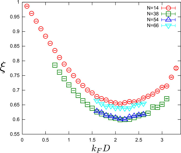
Figure 1: (Color online) Ratio between the variational energy per particle and the noninteracting Fermi gas energy as a function of the Jastrow term range. Results for $N=14$ ($\circ$), $N=38$ ($\square$), $N=54$ ($\triangle$), $N=66$ ($\triangledown$) particles.

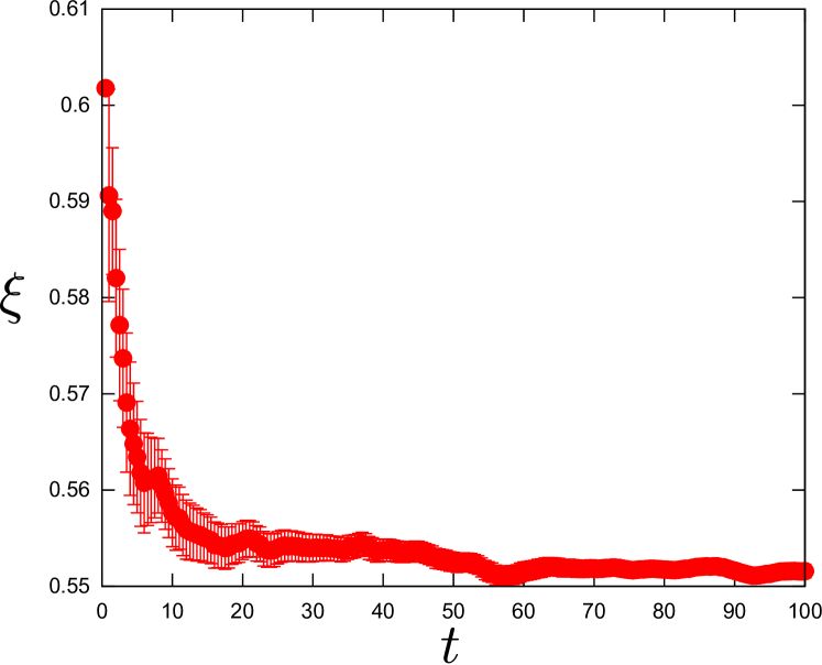
Figure 2: (Color online) Ratio between the energy per particle and the noninteracting Fermi gas energy as a function of the imaginary time in the DMC calculation. Results for $N=14$ particles. Each time step $\Delta t=10^{-3}\hbar/E_{FG}$.

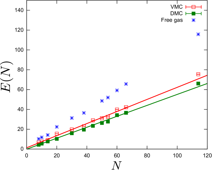
Figure 3: (Color online) The energy of the system as a function of the number of particles in the box. The red empty and green filled squares are the VMC and DMC energy results, respectively. Results for the non-interacting free gas are displayed for a comparison ( $\ast$). Energy in units of $E_{FG}$.

The Fig. 3 shows the ground state energies of the system as a function of the number of particles in the simulation. The red squares represent the variational results and the fitted straight red line results $E=0.61(2)E_{FG}$. The variational energy upper bound obtained by Chang and coworkers Chang et al. (2004) is $E=0.62(1)E_{FG}$ that is in good agreement with our result for the energy as expected for the similar forms for the trial wave functions. The main difference is our results do not need to be extrapolated to zero-range. The diffusion Monte Carlo energy is, of course, much lower. The green filled squares in the Fig. 3 show the energies for the diffusion Monte Carlo calculation evolving the Jastrow-Slater wave function in imaginary time. The fitted green straight line gives $E=0.55(1)E_{FG}$ in very good agreement with the available result from the literature Giorgini et al. (2008) $E=0.56(1)E_{FG}$ for the Slater-Jastrow wave function.

We have calculated the spin dependent pair correlation function. Fig. 4 shows the results for $g_{\uparrow\uparrow}(r)$ with a comparison with the non-interacting gas. For like spin pairs, the pair correlation function goes to zero at short distances because of the Pauli principle. The result for the non-interacting Fermi gas Astrakharchik et al. (2004) is described by

$$g_{\uparrow\uparrow}(r)=g_{\downarrow\downarrow}(r)=1-\frac{9}{(k_{F}r)^{4}}\left(\frac{\sin(k_{F}r)}{k_{F}r}-\cos(k_{F}r)\right)^{2}\;\;.$$ (23)

In the Fig. 4 one can see reasonable agreement between our results and the pair correlation function of the non-interacting Fermi gas, however the interaction modifies this and the result will be changed using diffusion Monte Carlo. As expected, $g_{\uparrow\downarrow}(r)$ has a $1/(k_{F}r)^{2}$ divergent behaviour when $r$ goes to zero Giorgini et al. (2008). Both $g_{\uparrow\downarrow}(r)$ and $g_{\uparrow\uparrow}(r)$ are normalized to go to $\frac{1}{2}$ at large distances.

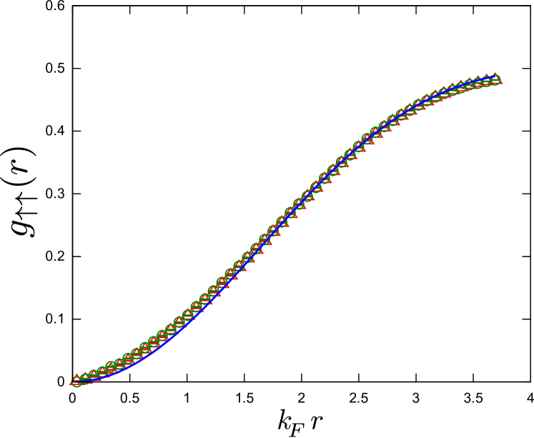
Figure 4: (Color online) Pair correlation function of like spin pairs calculated for $N=14$ particles. VMC and DMC results are represented by the green circles and the red triangles, respectively. The solid line shows the behaviour of the pair correlation function of the non-interacting Fermi gas Eq. (23).

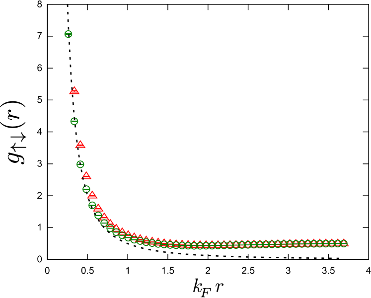
Figure 5: (Color online) Pair correlation function of unlike spin pairs for the system containing $N=14$ particles. VMC and DMC results are represented by the green circles and the red triangles, respectively. The dashed line is the function $1/(k_{F}r)^{2}$.

V Summary

In this work we have demonstrated that a system formed by ultracold fermions at the unitary regime can be studied using a zero-range interaction. In our Monte Carlo calculations we have devides variational trial wave functions with the correct boundary conditions, and we have developed improved sampling techniques to give a controlled variance in this zero-range limit.

The variational and diffusion Monte Carlo results are in good agreement with those reported in the literature for extrapolations of short but finite ranged potentials. We expect that our methods would could also be applied to improve the results with finite range potentials.

Further work optimizing the BCS wave functions can improve significantly the results reported in this paper. Automatic optimization of the BCS wave function for zero-range interactions as well as calculating other observables in ultracold Fermi gases is an ongoing.

References

- (1) E. Braaten, URL arXiv:1008.2922.
- Ketterle et al. (2008) W. Ketterle, W. Zwierlein, and S. italiana di fisica, Making, Probing and Understanding Ultracold Fermi Gases, Rivista del nuovo cimento (Societa italiana di fisica, 2008), URL http://arxiv.org/abs/0801.2500.
- Gandolfi et al. (2011) S. Gandolfi, K. E. Schmidt, and J. Carlson, Phys. Rev. A 83, 041601 (2011), URL http://link.aps.org/doi/10.1103/PhysRevA.83.041601.
- Giorgini et al. (2008) S. Giorgini, L. P. Pitaevskii, and S. Stringari, Rev. Mod. Phys. 80, 1215 (2008), URL http://link.aps.org/doi/10.1103/RevModPhys.80.1215.
- Carlson et al. (2003) J. Carlson, S.-Y. Chang, V. R. Pandharipande, and K. E. Schmidt, Phys. Rev. Lett. 91, 050401 (pages 4) (2003), URL http://link.aps.org/abstract/PRL/v91/e050401.
- Chang et al. (2004) S. Y. Chang, V. R. Pandharipande, J. Carlson, and K. E. Schmidt, Phys. Rev. A 70, 043602 (pages 11) (2004), URL http://link.aps.org/abstract/PRA/v70/e043602.
- Gezerlis and Carlson (2008) A. Gezerlis and J. Carlson, Phys. Rev. C 77, 032801 (2008), URL http://link.aps.org/doi/10.1103/PhysRevC.77.032801.
- Carlson and Reddy (2008) J. Carlson and S. Reddy, Phys. Rev. Lett. 100, 150403 (2008), URL http://link.aps.org/doi/10.1103/PhysRevLett.100.150403.
- Astrakharchik et al. (2005) G. Astrakharchik, J. Boronat, J. Casulleras, and S. Giorgini, Phys. Rev. Lett. 95, 230405 (2005), URL http://link.aps.org/doi/10.1103/PhysRevLett.95.230405.
- Astrakharchik et al. (2004) G. Astrakharchik, J. Boronat, J. Casulleras, and S. Giorgini, Phys. Rev. Lett. 93, 200404 (2004), URL http://link.aps.org/doi/10.1103/PhysRevLett.93.200404.
- Chang and Pandharipande (2005) S. Y. Chang and V. R. Pandharipande, Phys. Rev. Lett. 95, 080402 (2005), URL http://link.aps.org/doi/10.1103/PhysRevLett.95.080402.
- Tan (2008) S. Tan, Annals of Physics 323, 2952 (2008), ISSN 0003-4916, URL http://www.sciencedirect.com/science/article/pii/S00034916080%00456.
- Foulkes et al. (2001) W. M. C. Foulkes, L. Mitas, R. J. Needs, and G. Rajagopal, Rev. Mod. Phys. 73, 33 (2001).
- Kalos et al. (1974) M. H. Kalos, D. Levesque, and L. Verlet, Phys. Rev. A 9, 2178 (1974).
- Ceperley (1995) D. M. Ceperley, Rev. Mod. Phys. 67, 279 (1995).
- Metropolis et al. (1953) N. Metropolis, A. W. Rosenbluth, M. N. Rosenbluth, A. H. Teller, and E. Teller, The Journal of Chemical Physics 21, 1087 (1953), URL http://link.aip.org/link/?JCP/21/1087/1.
- Ceperley et al. (1977) D. M. Ceperley, G. V. Chester, and M. H. Kalos, Phys. Rev. B 16, 3081 (1977).
- Pudliner et al. (1997) B. S. Pudliner, V. R. Pandharipande, J. Carlson, S. C. Pieper, and R. B. Wiringa, Phys. Rev. C 56, 1720 (1997).