Measuring the Spin Polarization of a Ferromagnet: an Application of
Time-Reversal Invariant Topological Superconductor

Abstract

The spin polarization (SP) of the ferromagnet (FM) is a quantity of fundamental importance in spintronics. In this work, we propose a quasi-one-dimensional junction structure composed of a FM and a time-reversal invariant topological superconductor (TRITS) with un-spin-polarized pairing type to determine the SP of the FM. We find that due to the topological property of the TRITS, the zero-bias conductance (ZBC) of the FM/TRITS junction which is directly related to the SP is a non-quantized but topological quantity. The ZBC only depends on the parameters of the FM, it is independent of the interface scattering potential and the Fermi surface mismatch between the FM and the superconductor, and is robust against to the magnetic proximity effect, therefore, compared to the traditional FM/$s$-wave superconductor junction, the topological property of the ZBC makes this setup a much more direct and simplified way to determine the SP.

Introduction— Because of hosting exotic non-Abelian zero modes E. Majorana ; D. A. Ivanov which have great potential in topological quantum computation (TQC) Kitaev ; S. Das Sarma ; C. Nayak , topological superconductors (TSs) in every dimension have raised strong and lasting interests for more than a decade N. Read ; A. Kitaev ; G. E. Volovik ; Liang Fu ; C. W. Zhang ; M. Sato ; X.-L. Qi ; Y. Tanaka ; J. Linder ; Jay D. Sau ; Roman M. Lutchyn ; Y. Oreg ; J. Alicea1 ; A. C. Potter ; S. Sasaki ; S. Nakosai ; A. Keselman . Due to the nontrivial topology of the energy bands, TSs have many properties that are fundamentally different from the normal superconductors (NSs). One of the most remarkable difference is that the zero-bias conductance (ZBC) of a normal metal (NM)/TS junction is a quantized quantity of topological nature A. R. Akhmerov ; K. T. Law ; K. Flensberg , while for a NM/NS junction, the ZBC is parameter-dependent and can be greatly suppressed by the interface scattering potential G. E. Blonder .

As ferromagnet (FM) plays a crucial role in spintronics, the spin polarization (SP) of the FM is of fundamental importance S. A. Wolf ; I. Zutic . To determine the SP, a general approach is to detect the tunneling spectroscopy of the FM/$s$-wave superconductor junction R. J. Soulen ; S. K. Upadhyay ; Y. Ji ; G. J. Strijkers . The underlying mechanism is based on the fact that for a ballistic NM/$s$-wave superconductor junction, an electron with Fermi energy injected from the NM to the superconductor will be completely reflected as a hole with opposite spin, which is known as spin-opposite Andreev reflection A. F. Andreev , however, when the metal is a FM, due to the mismatch of the Fermi surface between the two spin degrees, some of the majority spin electrons can not undergo the spin-opposite Andreev reflection M. J. M. de Jong , instead, they are reflected as themselves, which is known as normal reflection, consequently, compared to the NM/$s$-wave superconductor junction, the conductance of the FM/$s$-wave superconductor junction is decreased, and the decrement monotonically increases with the mismatch increasing. As a result, the SP can be quantitatively determined by the tunneling spectroscopy.

Although the idea of the above mechanism is generally applied for every FM/$s$-wave superconductor junction, the concrete decrement can also be induced by other factors, such as the interface scattering potential and the Fermi surface mismatch between the FM and the superconductor Elina Tuuli . As a result, for general FM/$s$-wave superconductor junction, the tunneling spectroscopy may involve many parameters, and consequently, the SP is very hard to be precisely resolved from the tunneling spectroscopy I. I. Mazin1 ; T. Y. Chen . However, in this work, we find that if the normal $s$-wave superconductor is substituted by a time-reversal invariant (TRI) TS with un-spin-polarized pairing type, then as the ZBC turns out to be a topological quantity only related to the parameters of the FM, the process to determine the SP becomes much more direct and simplified.

Theoretical model— So far, the greatest experimental progress made on the transport study of TS is in one dimension V. Mourik ; A. Das ; M. T. Deng ; A. D. K. Finck ; L. P. Rokhinson ; S. Nadj-Perge . For generality, in this work we consider the FM is a quasi-one-dimensional wire, with length $L$ in $x$-direction and width $W$ in $y$-direction, and $L>>W$. Correspondingly, for the TS, the width is also given by $W$, and the length is assumed to be infinite for simplicity. Then the Hamiltonian describing the junction under the representation $\hat{\Psi}^{{\dagger}}(x,y)=(\hat{\psi}^{{\dagger}}_{\uparrow}(x,y),\hat{\psi}_{\downarrow}(x,y),\hat{\psi}^{{\dagger}}_{\downarrow}(x,y),\hat{\psi}_{\uparrow}(x,y))$ is given by

$$\mathcal{H}=\tau_{z}\left[-\frac{\hbar^{2}}{2m}(\partial^{2}_{x}+\partial^{2}_{y})-\mu(x,y)+V(x,y)\right]+\tau_{x}\Delta(x,y),$$ (1)

where $\vec{\tau}=(\tau_{x},\tau_{y},\tau_{z})$ are Pauli matrices in particle-hole space, $V(x,y)$ is potential induced by disorder, external field, $etc$, here we assume it takes the form $-M\tau_{z}\sigma_{z}\Theta(-x)+V\delta(x)$, the former term denotes the magnetization of the FM, $\sigma_{z}$ is a Pauli matrix acting on the spin space, $\Theta(-x)$ is the Heaviside function, the latter term denotes the scattering potential at the interface. $\mu(x,y)$ is the chemical potential, we set $\mu(x,y)=\mu_{f}$ (or $E_{F}$) for the ferromagnetic part ($x<0$) and $\mu(x,y)=\mu_{s}$ for the superconductor ($x>0$). $\Delta(x,y)=-i\Delta_{0}\Theta(x)\partial_{x}$ is the pairing potential, which is assumed to be $p$-wave type and homogeneous at $x>0$ and vanish at $x<0$ for the sake of theoretical simplicity. The mass $m$ of the particle is assumed to be positive and the same throughout the system.

As the system is strongly confined in $y$-direction, the system will form a series of subbands with band index $n$ a good quantum number. Then the field operator can be expressed as $\hat{\psi}_{\sigma}(x,y)=\sum_{n}\hat{\psi}_{n\sigma}(x)\chi_{n}(y)$, where $\chi_{n}(y)=\sqrt{\frac{2}{W}}\sin(k_{n}y)$, with $k_{n}=n\pi/W$. By a Fourier transformation $\hat{\psi}_{n\sigma}(x)=\int\frac{dk}{2\pi}e^{ikx}\hat{c}_{n\sigma,k}$, the Hamiltonians for the ferromagnetic part and the superconducting part under the representation $\hat{\Psi}^{{\dagger}}_{nk}=(\hat{c}_{n\uparrow,k}^{{\dagger}},\hat{c}_{n\downarrow,-k},\hat{c}_{n\downarrow,k}^{{\dagger}},\hat{c}_{n\uparrow,-k})$ are given as

$$\mathcal{H}_{F}(k)=[\frac{\hbar^{2}k^{2}}{2m}+\epsilon_{n}-\mu_{f}]\tau_{z}-M\tau_{0}\sigma_{z},$$

$$\mathcal{H}_{S}(k)=[\frac{\hbar^{2}k^{2}}{2m}+\epsilon_{n}-\mu_{s}]\tau_{z}+\Delta(k)\tau_{x},$$ (2)

respectively, where $\epsilon_{n}=n^{2}\hbar^{2}\pi^{2}/(2mW^{2})$, $\Delta(k)=\Delta_{0}k$. As $\tau_{z}\mathcal{H}_{S}(k)\tau_{z}=\mathcal{H}_{S}^{*}(-k)$, $\tau_{x}\mathcal{H}_{S}(k)\tau_{x}=-\mathcal{H}_{S}^{*}(-k)$, $\tau_{y}\mathcal{H}_{S}(k)\tau_{y}=-\mathcal{H}_{S}(k)$, and $(\tau_{z}K)^{2}=1$, $\mathcal{H}_{S}(k)$ belongs to the BDI class A. P. Schnyder ; A. Y. Kitaev . From Eq.(2), it is direct to obtain the excitation energy spectra of the FM, $E_{fn\uparrow(\downarrow)}=\hbar^{2}k^{2}/2m+\epsilon_{n}-\mu_{f}\mp M$, then the particle number partition $(N_{\uparrow},N_{\downarrow})$ can be directly obtained as $N_{\uparrow}=(L/\pi)\sum_{n}^{{}^{\prime}}\sqrt{2m(\mu_{f}+M-\epsilon_{n})}$, $N_{\downarrow}=(L/\pi)\sum_{n}^{{}^{\prime\prime}}\sqrt{2m(\mu_{f}-M-\epsilon_{n})}$, where the two superscripts mean that the two summations are limited by two upper limit $n^{{}^{\prime}}$ and $n^{{}^{\prime\prime}}$, respectively. $n^{{}^{\prime}}$ satisfies $(\mu_{f}+M-\epsilon_{n^{{}^{\prime}}})>0$ and $(\mu_{f}+M-\epsilon_{n^{{}^{\prime}}+1})<0$, similarly $n^{{}^{\prime\prime}}$ satisfies $(\mu_{f}-M-\epsilon_{n^{{}^{\prime\prime}}})>0$ and $(\mu_{f}-M-\epsilon_{n^{{}^{\prime\prime}}+1})<0$. If the particle number partition $(N_{\uparrow},N_{\downarrow})$ is known, the SP, which is defined as I. I. Mazin2

$$P \equiv \frac{\sum_{n}^{{}^{\prime}}N_{n\uparrow}(E_{F})v_{F,n\uparrow}^{2}-\sum_{n}^{{}^{\prime\prime}}N_{n\downarrow}(E_{F})v_{F,n\downarrow}^{2}}{\sum_{n}^{{}^{\prime}}N_{n\uparrow}(E_{F})v_{F,n\uparrow}^{2}+\sum_{n}^{{}^{\prime\prime}}N_{n\downarrow}(E_{F})v_{F,n\downarrow}^{2}}$$ (3)

$$= \frac{N_{\uparrow}-N_{\downarrow}}{N_{\uparrow}+N_{\downarrow}},$$

where $N_{n\sigma}(E_{F})$ is the density of states at the Fermi energy and $v_{F,n\sigma}$ is the Fermi velocity, can be directly obtained. Note that in the quasi-one-dimensional case, as $N_{n\uparrow}(E_{F})v_{F,n\uparrow}=N_{n\downarrow}(E_{F})v_{F,n\downarrow}=const$, the ballistic definition $P=(N_{\uparrow}(E_{F})v_{F\uparrow}-N_{\downarrow}(E_{F})v_{F\downarrow})/(N_{\uparrow}(E_{F})v_{F\uparrow}+N_{\downarrow}(E_{F})v_{F\downarrow})$ does not apply R. J. Soulen . For the superconducting part, the quasi-particle energy spectra is given as $E_{sn}=\sqrt{(\hbar^{2}k^{2}/2m+\epsilon_{n}-\mu_{s})^{2}+\Delta_{0}^{2}k^{2}}$. When $\mu_{s}-\epsilon_{n}>0$, the bands with index smaller than $n+1$ are all of nontrivial topology B. A. Bernevig . In this work, we first consider $\epsilon_{1}<\mu_{s}<\epsilon_{2}$, in other words, only bands with index $n=1$ are of nontrivial topology.

Relation between ZBC and SP— Due to the orthogonality of $\{\chi_{n}(y)\}$, if an electron with spin-up, excitation energy $E$ and band index $n$ is injected from the FM, the wave function in the FM is given as $\psi_{f,n}(x<0)=\vec{e}_{1}e^{iq_{n\uparrow,e}x}+b_{n\uparrow}\vec{e}_{1}e^{-iq_{n\uparrow,e}x}+a_{n\downarrow}\vec{e}_{2}e^{iq_{n\downarrow,h}x}+b_{n\downarrow}\vec{e}_{3}e^{-iq_{n\downarrow,e}x}+a_{n\uparrow}\vec{e}_{4}e^{iq_{n\uparrow,h}x}$, where $\vec{e}_{1}=(1,0,0,0)^{T}$, $\vec{e}_{2}=(0,1,0,0)^{T}$ $\vec{e}_{3}=(0,0,1,0)^{T}$, and $\vec{e}_{4}=(0,0,0,1)^{T}$. $q_{n\uparrow,e}(E)=\sqrt{2m(\mu_{f}+M+E-\epsilon_{n})}$, $q_{n\downarrow,h}(E)=\sqrt{2m(\mu_{f}-M-E-\epsilon_{n})}$, $q_{n\downarrow,e}(E)=\sqrt{2m(\mu_{f}-M+E-\epsilon_{n})}$, and $q_{n\uparrow,h}(E)=\sqrt{2m(\mu_{f}+M-E-\epsilon_{n})}$. $b_{n\uparrow}$ and $b_{n\downarrow}$ denote the amplitudes corresponding to spin-equal and spin-opposite normal reflection, respectively. $a_{n\uparrow}$ and $a_{n\downarrow}$ denote the amplitudes corresponding to spin-equal and spin-opposite Andreev reflection, respectively. In this work, we are only interested in the special case with $E=0$. When $E=0$, the wave function in the superconductor is very simple. If $n=1$, corresponding to the band of nontrivial topology, $\psi_{s,n}(x>0)=c_{n1}\vec{e}_{5}e^{-k_{n+}x}+d_{n1}\vec{e}_{5}e^{-k_{n-}x}+c_{n2}\vec{e}_{6}e^{-k_{n+}x}+d_{n2}\vec{e}_{6}e^{-k_{n-}x}$, where $\vec{e}_{5}=(i,1,0,0)^{T}$ and $\vec{e}_{6}=(0,0,i,1)^{T}$. While for $n\geq 2$, corresponding to the bands of trivial topology, $\psi_{s,n}(x>0)=c_{n1}\vec{e}_{5}e^{-k_{n+}x}+d_{n1}\vec{e}_{7}e^{-k_{n-}x}+c_{n2}\vec{e}_{6}e^{-k_{n+}x}+d_{n2}\vec{e}_{8}e^{-k_{n-}x}$, where $\vec{e}_{7}=(-i,1,0,0)^{T}$ and $\vec{e}_{8}=(0,0,-i,1)^{T}$. As $k_{n+}$ and $k_{n-}$ will not show up in the results, we do not write down their expressions explicitly here.

If the superconductor is only weak pairing which means that only when the band minimum is lower than $\mu_{s}$, the band is metallic and has states to pair to be superconducting B. A. Bernevig , we only need to consider the $n=1$ bands. However, for generality, here we consider all bands are paired to be superconducting.

Again due to the orthogonality of $\{\chi_{n}(y)\}$, the boundary conditions of the wave functions at the interface is given as Z. B. Yan

$$\psi_{f,n}(0)=\psi_{s,n}(0),$$

$$v_{s}\psi_{s,n}(0^{+})-v_{f}\psi_{f,n}(0^{-})=-iZ\tau_{z}\sigma_{0}\psi_{s,n}(0),$$ (4)

where $v_{s}=\partial_{k}\mathcal{H}_{S}/\hbar$, $v_{f}=\partial_{k}\mathcal{H}_{F}/\hbar$, $Z=2V/\hbar$. Based on Eq.(4), all coefficients can be directly obtained, and then according to the Blonder-Tinkham-Klapwijk formula G. E. Blonder , the ZBC is given as

$$G(0)=\frac{e^{2}}{h}\sum_{n_{\pm}}(1+A_{n_{\pm}\uparrow}+A_{n_{\pm}\downarrow}-B_{n_{\pm}\uparrow}-B_{n_{\pm}\downarrow}),$$ (5)

where $+$(-) denotes that the injected electron is spin-up (spin-down). The summation on majority spin band number $n_{+}$ (minority spin band number $n_{-}$) goes from $1$ to $n^{{}^{\prime}}$ ($n^{{}^{\prime\prime}}$). $A_{n_{+}\uparrow}=q_{n\uparrow,h}(0)|a_{n\uparrow}|^{2}/q_{n\uparrow,e}(0)$, $B_{n_{+}\uparrow}=|b_{n\uparrow}|^{2}$, $A_{n_{+}\downarrow}=q_{n\downarrow,h}(0)|a_{n\downarrow}|^{2}/q_{n\uparrow,e}(0)$, $B_{n_{+}\downarrow}=q_{n\downarrow,e}(0)|b_{n\downarrow}|^{2}/q_{n\uparrow,e}(0)$, $A_{n_{-}\uparrow}=q_{n\uparrow,h}(0)|a_{n\uparrow}|^{2}/q_{n\downarrow,e}(0)$, $B_{n_{-}\downarrow}=|b_{n\downarrow}|^{2}$, $A_{n_{-}\downarrow}=q_{n\downarrow,h}(0)|a_{n\downarrow}|^{2}/q_{n\downarrow,e}(0)$, $B_{n_{-}\uparrow}=q_{n\uparrow,e}(0)|b_{n\uparrow}|^{2}/q_{n\downarrow,e}(0)$. Due to the current conservation, these quantities satisfy the constraint: $A_{n_{\pm}\uparrow}+A_{n_{\pm}\downarrow}+B_{n_{\pm}\downarrow}+B_{n_{\pm}\downarrow}=1$. This constraint can simplify the conductance formula as

$$G(0)=\frac{2e^{2}}{h}\sum_{n_{\pm}}(A_{n_{\pm}\uparrow}+A_{n_{\pm}\downarrow}).$$ (6)

Based on Eq.(4), a direct calculation shows that $A_{n_{+}\uparrow}$ and $A_{n_{-}\downarrow}$ always vanish and SM

$$A_{n_{+}\downarrow}=A_{n_{-}\uparrow}=\left\{\begin{array}[]{cc}\frac{4q_{n\uparrow}q_{n\downarrow}}{(q_{n\uparrow}+q_{n\downarrow})^{2}},&n=1\\ 0,&n\geq 2.\end{array}\right.$$ (9)

where $q_{n\uparrow(\downarrow)}=q_{n\uparrow(\downarrow),e}(0)=q_{n\uparrow(\downarrow),h}(0)$. $A_{n_{+}\uparrow}$ and $A_{n_{-}\downarrow}$, both denoting the spin-equal Andreev reflection, taking value zero is a natural result since the superconductor is with un-spin-polarized pairing type. The non-vanishing quantities only depend on the parameters of the FM, they are independent of the scattering potential and the parameters of the superconductor, which suggests that they are of topological nature. Substituting Eq.(9) into Eq.(6), it is direct to obtain

$$\bar{G}(0)\equiv\frac{hG(0)}{e^{2}}=\frac{16q_{1\uparrow}q_{1\downarrow}}{(q_{1\uparrow}+q_{1\downarrow})^{2}}.$$ (10)

The zero-bias conductance is only related to the lowest spin-up and spin-down subband of the FM. As a result, it is found that only in the strict one-dimensional limit, $G(0)$ has enough information to directly determine the polarization of the FM. In the strict one-dimensional limit, $i.e.$, $\epsilon_{1}<\mu_{f}$ and $\mu_{f}-\epsilon_{1}<<\epsilon_{2}$, the particle number for each spin is given as: $N_{\uparrow}=Lq_{1\uparrow}/\pi$, $N_{\uparrow}=Lq_{1\downarrow}/\pi$. As a result, $\bar{G}(0)=16N_{\uparrow}N_{\downarrow}/(N_{\uparrow}+N_{\downarrow})^{2}$. Combining this result with Eq.(3), it is direct to obtain

$$P=\sqrt{1-\frac{\bar{G}(0)}{4}}.$$ (11)

If the superconductor is a normal $s$-wave superconductor, the ZBC in the strict one-dimensional limit is given as SM

$$\tilde{G}(0)=\frac{e^{2}}{h}\frac{16\kappa^{2}q_{1\downarrow}q_{1\uparrow}}{(\kappa^{2}+q_{1\uparrow}q_{1\downarrow}+\bar{Z}^{2})^{2}+\bar{Z}^{2}(q_{1\downarrow}-q_{1\uparrow})^{2}},$$ (12)

where $\kappa\simeq\sqrt{2m\mu_{s}}$, and $\bar{Z}=mZ/\hbar$. As $\tilde{G}(0)$ involves parameters of all three parts: the FM, the superconductor, and the interface, the resolution of SP from $\tilde{G}(0)$, if not possible, is very complicated I. I. Mazin1 ; T. Y. Chen . It is found that only in the clean limit and without mismatch of Fermi surface between the FM and the superconductor, SP can be directly determined by $\tilde{G}(0)$ through the formula

$$P=\left(1-\frac{\bar{\tilde{G}}(0)}{4}\right)^{\frac{1}{4}},$$ (13)

where $\bar{\tilde{G}}(0)\equiv h\tilde{G}(0)/e^{2}$. Any one of the two ideal conditions in real junctions is in fact hardly to satisfy. All of these suggest that compared to the FM/$s$-wave superconductor junction, the topological property of $\bar{G}(0)$ makes the resolution of SP from the FM/TRITS junction much more direct and simplified, simultaneously with an improvement of the precision.

When the number of subbands for spin-up and spin-down are both larger than one, the simple formula (11) is obviously no longer valid. However, $\bar{G}(0)$ can still provide important information about the SP. By defining a quantity as $\eta\equiv M/(\mu_{f}-\epsilon_{1})$, which is the relative strength of the magnetization, it is direct to find

$$\eta=\frac{4\sqrt{4-\bar{G}(0)}}{4+(4-\bar{G}(0))}.$$ (14)

If we further define a quantity as $\lambda=\epsilon_{1}/(\mu_{f}-\epsilon_{1})$, then the particle number for each spin can be expressed as: $N_{\uparrow}=(Lk_{f}/\pi)\sum_{n}^{{}^{\prime}}\sqrt{1+\eta-(n^{2}-1)\lambda}$, $N_{\downarrow}=(Lk_{f}/\pi)\sum_{n}^{{}^{\prime\prime}}\sqrt{1-\eta-(n^{2}-1)\lambda}$, with $k_{f}=\sqrt{2m(\mu_{f}-\epsilon_{1})}$. Therefore, if the value of $\lambda$ is known, the SP in fact can also be deduced from $\bar{G}(0)$. As $\epsilon_{1}$ can easily be determined by measuring the width of the ferromagnetic metal (if $m$ is known), the only residual challenge is to determine $\mu_{f}$. However, if there are at least two subbands occupied by the minority spin electrons, in fact we can easily determine $\lambda$ in the same setup by just tuning $\mu_{s}$.

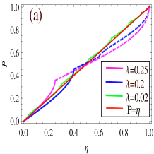
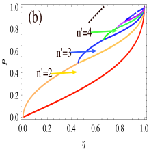
Figure 1: (color online) Polarization-$vs$-magnetization. (a) The dashed parts of the lines are where $\eta>1-3\lambda$, and as a result, $\lambda$ can not be determined from Eq.(13) due to $\delta\bar{G}(0)=0$. (b) With $n^{{}^{\prime\prime}}$ fixed to $1$, the region closed by two neighbor lines corresponds to the possible value of the polarization for certain $n^{{}^{\prime}}$.

As $\lambda$ enters into $N_{\uparrow}$ and $N_{\downarrow}$ through terms with $n\geq 2$, we can tune $\mu_{s}$ from the region $(\epsilon_{1},\epsilon_{2})$ to $(\epsilon_{2},\epsilon_{3})$. When $\mu_{s}$ goes across $\epsilon_{2}$, there is a jump in ZBC, with $\delta\bar{G}(0)=16q_{2\uparrow}q_{2\downarrow}/(q_{2\uparrow}+q_{2\downarrow})^{2}$, then a direct calculation gives

$$\lambda=\frac{1}{3}\left[1-\sqrt{\left(\frac{\delta\bar{G}(0)}{8-\delta\bar{G}(0)}\right)^{2}+\eta^{2}}\,\right].$$ (15)

In Fig.1(a), it is shown that when $\lambda<<1$ (many bands occupied), the formula (15) is almost valid in the whole region of $\eta$, and $P$ is well approximated by $\eta$, $i.e.$, $P\simeq\eta$, this is a very useful result for experiments.

If the number of occupied subbands is large, but the magnetization is so strong that it makes $1>\eta>1-3\lambda$, then as $n^{{}^{\prime\prime}}=1$, $\delta\bar{G}(0)$ is always equal to zero, the above approach to determine $\lambda$ breaks down. For this case, as shown in Fig.1(b), what we can be precisely determined is the upper limit ($P_{u}$) and lower limit ($P_{l}$) of the polarization. To character the uncertainty of the polarization, we define a quantity as $\Delta\bar{P}=2(P_{u}-P_{l})/(P_{u}+P_{l})$. When $n^{{}^{\prime\prime}}=1$, $n^{{}^{\prime}}=2$, in the weak magnetization region, it is found that $\Delta\bar{P}$ can go beyond $100\%$. However, with $n^{{}^{\prime}}$ increasing, $\Delta\bar{P}$ decreases very fast. When $n^{{}^{\prime}}\geq 5$, we can take the boundary value $P_{u}$ or $P_{l}$, or $\eta$, as the precise value of the SP. To determine the number of the subbands for the majority spin electrons, we only need to detect the ZBC of the FM. If the FM is sufficiently clean to guarantee $W<<L<l$, where $l$ is the mean free path, the quantized ZBC is given as $G(0)=(n^{{}^{\prime}}+n^{{}^{\prime\prime}})e^{2}/h$.

The three cases analyzed above exhaust all possibilities. For most cases, due to the topological nature of $\bar{G}(0)$ and $\delta\bar{G}(0)$, the polarization can be easily and precisely determined by this . Only in the parameter region: $n^{{}^{\prime\prime}}=1$, $2\leq n^{{}^{\prime}}\leq 4$, the precision is not very good. If with the help of other measurements, both $\epsilon_{1}$ and $\mu_{f}$ are precisely determined, of course then $P$ can be directly and precisely determined by the simple quantity $\bar{G}(0)$ for all cases.

Magnetic proximity effect— When a FM is in proximity to a superconductor, the magnetization of the FM is equivalent to a magnetic field, and it will penetrate into the superconductor and break Cooper pairs within the magnetic penetration depth. However, this pair-breaking effect should not affect the validity of the three formulae (11)(14)(15), because the penetration is a local behavior, it should not affect the topological property of the superconductor. In fact, in real experiments, this pair-breaking effect can be avoided or greatly reduced by adding a finite-thickness insulator between the FM and the superconductor. It is found that no matter how thick the insulator is, when $\epsilon_{1}<\mu_{s}<\epsilon_{2}$, $\bar{G}(0)$ is always given by the formula (10) SM . Although $\bar{G}(0)$ does not depend on the thickness of the insulator, the width of $\bar{G}(eV)$ will exponentially decrease with the thickness. Therefore, for the sake of observing the peak and detecting its value, a proper choice of the thickness is needed.

Experimental realization— Compared to the TRI $p$-wave superconductor with un-spin-polarized pairing type that belongs to the BDI class, a TRI $d$-wave TS is in fact more experimentally realizable C. L. M. Wong ; Z. Yan . Similar to the semiconductor-based proposal of TS Roman M. Lutchyn ; Y. Oreg , a TRI $d$-wave TS can also be realized by making a semiconductor wire with intrinsic spin-orbit coupling in proximity to a $d$-wave superconductor C. L. M. Wong . Both materials are common in reality. As the TRI $d$-wave TS belongs to the DIII class, it can only host at most one subband (without considering degeneracy) of nontrivial topology. To determine both $\bar{G}(0)$ and $\lambda$, we can first tune $\mu_{s}$ to make only the lowest subband to be topological and obtain $\bar{G}(0)$, and then tune $\mu_{s}$ to make only the second-lowest subband to be topological and obtain $\bar{G}^{\prime}(0)=\delta\bar{G}(0)$ SM .

Conclusions— The independence of $Z$ and the robustness against magnetic proximity effect make the ZBC an observable that can easily and directly determine the SP of a FM. This points out another potential application of TS besides its well-known potential application in TQC.

Acknowledgments.— This work was supported by NSFC Grant No.11275180.

I Supplementary Materials

I.0.1 I. Ferromagnet/$s$-wave superconductor junction

For a one-dimensional ferromagnet (FM)/$s$-wave superconductor junction, the Hamiltonians describing the FM and the $s$-wave superconductor under the representation $\hat{\Psi}^{{\dagger}}_{k}=(\hat{c}_{\uparrow,k}^{{\dagger}},\hat{c}_{\downarrow,-k},\hat{c}_{\downarrow,k}^{{\dagger}},-\hat{c}_{\uparrow,-k})$ are given as

$$\mathcal{H}_{F}(k)=[\frac{\hbar^{2}k^{2}}{2m}-\mu_{f}]\tau_{z}-M\tau_{0}\sigma_{z},$$

$$\mathcal{H}_{S}(k)=[\frac{\hbar^{2}k^{2}}{2m}-\mu_{s}]\tau_{z}+\Delta\tau_{x},$$ (16)

respectively. When a spin-up electron with the Fermi energy is injected from the FM to the superconductor, if we assume that the FM corresponds to the $x<0$ part, while the superconductor corresponds to the $x>0$ part, the general wave function in the FM is given as

$$\psi_{f}(x)=\left(\begin{array}[]{c}1\\ 0\\ 0\\ 0\\ \end{array}\right)e^{iq_{\uparrow}x}+b_{\uparrow}\left(\begin{array}[]{c}1\\ 0\\ 0\\ 0\\ \end{array}\right)e^{-iq_{\uparrow}x}+a_{\downarrow}\left(\begin{array}[]{c}0\\ 1\\ 0\\ 0\\ \end{array}\right)e^{iq_{\downarrow}x}+b_{\downarrow}\left(\begin{array}[]{c}0\\ 0\\ 1\\ 0\\ \end{array}\right)e^{-iq_{\downarrow}x}+a_{\uparrow}\left(\begin{array}[]{c}0\\ 0\\ 0\\ 1\\ \end{array}\right)e^{iq_{\uparrow}x},$$ (37)

where $q_{\uparrow}=\sqrt{2m(\mu_{f}+M)}$, $q_{\downarrow}=\sqrt{2m(\mu_{f}-M)}$. $b_{\uparrow(\downarrow)}$ denotes the amplitude that the injected electron is reflected as a spin-up (spin-down) electron, and $a_{\uparrow(\downarrow)}$ denotes the amplitude that the injected electron is reflected as a spin-up (spin-down) hole. The general wave function in the superconductor is given as

$$\psi_{s}(x)=c_{1}\left(\begin{array}[]{c}i\\ 1\\ 0\\ 0\\ \end{array}\right)e^{i\kappa x-\gamma x}+d_{1}\left(\begin{array}[]{c}-i\\ 1\\ 0\\ 0\\ \end{array}\right)e^{-i\kappa x-\gamma x}+c_{2}\left(\begin{array}[]{c}0\\ 0\\ i\\ 1\\ \end{array}\right)e^{i\kappa x-\gamma x}+d_{2}\left(\begin{array}[]{c}0\\ 0\\ -i\\ 1\\ \end{array}\right)e^{-i\kappa x-\gamma x},$$ (54)

where $\kappa=\left(\sqrt{2m\sqrt{\mu_{s}^{2}+\Delta^{2}}+2m\Delta}+\sqrt{2m\sqrt{\mu_{s}^{2}+\Delta^{2}}-2m\Delta}\right)/2$, $\gamma=\left(\sqrt{2m\sqrt{\mu_{s}^{2}+\Delta^{2}}+2m\Delta}-\sqrt{2m\sqrt{\mu_{s}^{2}+\Delta^{2}}-2m\Delta}\right)/2$. By matching the wave function at $x=0$ according to the boundary conditions

$$\psi_{f}(0)=\psi_{s}(0),$$

$$v_{s}\psi_{s}(0^{+})-v_{f}\psi_{f}(0^{-})=-iZ\tau_{z}\sigma_{0}\psi_{s}(0),$$ (55)

where $v_{s}=\partial_{k}\mathcal{H}_{s}/\hbar$, $v_{f}=\partial_{k}\mathcal{H}_{f}/\hbar$, whose concrete expressions are given as

$$v_{s}=v_{n}=\frac{\hbar}{m}\left(\begin{array}[]{cccc}k&0&0&0\\ 0&-k&0&0\\ 0&0&k&0\\ 0&0&0&-k\\ \end{array}\right)=\frac{-i\hbar}{m}\left(\begin{array}[]{cccc}\partial_{x}&0&0&0\\ 0&-\partial_{x}&0&0\\ 0&0&\partial_{x}&0\\ 0&0&0&-\partial_{x}\\ \end{array}\right),$$ (64)

and $Z$ denotes the interface scattering potential, we obtain a series of algebraic relation between the coefficients,

$$1+b_{\uparrow}=i(c_{1}-d_{1}),$$

$$a_{\downarrow}=c_{1}+d_{1},$$

$$b_{\downarrow}=i(c_{2}-d_{2}),$$

$$a_{\uparrow}=c_{2}+d_{2},$$

$$ic_{1}(\kappa+i\gamma)+id_{1}(\kappa-i\gamma)-q_{\uparrow}(1-b_{\uparrow})=-i\bar{Z}(1+b_{\uparrow}),$$

$$-c_{1}(\kappa+i\gamma)+d_{1}(\kappa-i\gamma)+q_{\downarrow}a_{\downarrow}=i\bar{Z}a_{\downarrow},$$

$$ic_{2}(\kappa+i\gamma)+id_{2}(\kappa-i\gamma)+q_{\downarrow}b_{\downarrow}=-i\bar{Z}b_{\downarrow},$$

$$-c_{2}(\kappa+i\gamma)+d_{2}(\kappa-i\gamma)+q_{\uparrow}a_{\uparrow}=i\bar{Z}a_{\uparrow},$$ (65)

where $\bar{Z}=mZ/\hbar$. A direct calculation gives

$$b_{\uparrow}=-\frac{\kappa^{2}-q_{\uparrow}q_{\downarrow}+(\gamma+\bar{Z})^{2}+i(\gamma+\bar{Z})(q_{\uparrow}+q_{\downarrow})}{\kappa^{2}+q_{\uparrow}q_{\downarrow}+(\gamma+\bar{Z})^{2}+i(\gamma+\bar{Z})(q_{\downarrow}-q_{\uparrow})},$$

$$a_{\downarrow}=-\frac{2i\kappa q_{\uparrow}}{\kappa^{2}+q_{\uparrow}q_{\downarrow}+(\gamma+\bar{Z})^{2}+i(\gamma+\bar{Z})(q_{\downarrow}-q_{\uparrow})},$$

$$c_{1}=-\frac{iq_{\uparrow}(\kappa+q_{\downarrow}-i(\gamma+\bar{Z}))}{\kappa^{2}+q_{\uparrow}q_{\downarrow}+(\gamma+\bar{Z})^{2}+i(\gamma+\bar{Z})(q_{\downarrow}-q_{\uparrow})},$$

$$d_{1}=-\frac{iq_{\uparrow}(\kappa-q_{\downarrow}+i(\gamma+\bar{Z}))}{\kappa^{2}+q_{\uparrow}q_{\downarrow}+(\gamma+\bar{Z})^{2}+i(\gamma+\bar{Z})(q_{\downarrow}-q_{\uparrow})},$$

$$b_{\downarrow}=a_{\uparrow}=c_{2}=d_{2}=0.$$ (66)

As the wave function in the superconductor decays with $x$ increasing, the non-vanishing two quantities $c_{1}$ and $d_{1}$ also have no contribution to the current. Therefore, the current conservation needs: $A_{\downarrow}+B_{\uparrow}=q_{\downarrow}|a_{\downarrow}|^{2}/q_{\uparrow}+|b_{\uparrow}|^{2}=1$, which is easy to be verified. Then according to the Blonder-Tinkham-Klapwijk (BTK) formula G. E. Blonder1 , the zero-bias conductance (ZBC) is given as

$$G_{\uparrow}(0)=\frac{e^{2}}{h}(1+A_{\downarrow}-B_{\uparrow})=2\frac{e^{2}}{h}A_{\downarrow}.$$ (67)

Similar procedures for the spin-down case will show that $G_{\downarrow}(0)=G_{\uparrow}(0)$, and therefore, the measured ZBC is given as

$$G(0) = G_{\downarrow}(0)+G_{\uparrow}(0)$$ (68)

$$= \frac{e^{2}}{h}\frac{16\kappa^{2}q_{\downarrow}q_{\uparrow}}{(\kappa^{2}+q_{\uparrow}q_{\downarrow}+(\gamma+\bar{Z})^{2})^{2}+(\gamma+\bar{Z})^{2}(q_{\downarrow}-q_{\uparrow})^{2}}.$$

As generally $\mu_{s}>>\Delta$, $\kappa\simeq k_{F}=\sqrt{2m\mu_{s}}$, $\gamma\simeq\frac{\Delta}{\mu_{s}}k_{F}<<\kappa$, $\gamma$ can be safely neglected, then $G(0)$ is simplified as

$$G(0)=\frac{e^{2}}{h}\frac{16\kappa^{2}q_{\downarrow}q_{\uparrow}}{(\kappa^{2}+q_{\uparrow}q_{\downarrow}+\bar{Z}^{2})^{2}+\bar{Z}^{2}(q_{\downarrow}-q_{\uparrow})^{2}}.$$ (69)

$G(0)$ depends on the parameters of all three parts: the FM, the superconductor, and the interface. It is obvious that the resolution of the spin polarization (SP) from $G(0)$ if not possible, is very hard and complicated. In fact, only in the clean limit and without mismatch of the Fermi surface between the FM and the superconductor, $i.e.$, $\bar{Z}=0$ and $\mu_{s}=\mu_{f}$, $G(0)$ can directly determine the SP. Under the two idea conditions, $G(0)$ is simplified as

$$G(0)=\frac{e^{2}}{h}\frac{16\sqrt{1-\bar{\eta}^{2}}}{(1+\sqrt{1-\bar{\eta}^{2}})^{2}},$$ (70)

where $\bar{\eta}=M/\mu_{f}$. Then as $P=\frac{\sqrt{1+\bar{\eta}}-\sqrt{1-\bar{\eta}}}{\sqrt{1+\bar{\eta}}+\sqrt{1-\bar{\eta}}}$, a direct calculation gives

$$P=\left[1-\frac{\bar{G}(0)}{4}\right]^{\frac{1}{4}},$$ (71)

where $\bar{G(0)}=hG(0)/e^{2}$.

I.0.2 II. Ferromagnet/TRI $p$-wave superconductor with pairing type $(|\uparrow\downarrow>+\downarrow\uparrow>)$ junction

This junction is the case we have considered in the main text. The junction is quasi-one-dimensional with width $W$, and the Hamiltonians describing the FM and the superconductor under the representation $\hat{\Psi}^{{\dagger}}_{nk}=(\hat{c}_{n\uparrow,k}^{{\dagger}},\hat{c}_{n\downarrow,-k},\hat{c}_{n\downarrow,k}^{{\dagger}},\hat{c}_{n\uparrow,-k})$ are given as

$$\mathcal{H}_{F}(k)=[\frac{\hbar^{2}k^{2}}{2m}+\epsilon_{n}-\mu_{f}]\tau_{z}-M\tau_{0}\sigma_{z},$$

$$\mathcal{H}_{pS}(k)=[\frac{\hbar^{2}k^{2}}{2m}+\epsilon_{n}-\mu_{s}]\tau_{z}+\Delta(k)\tau_{x},$$ (72)

respectively, where $\epsilon_{n}=n^{2}\hbar^{2}\pi^{2}/(2mW^{2})$, $\Delta(k)=\Delta_{0}k$. With the assumption $\epsilon_{1}<\mu_{s}<\epsilon_{2}$, when an spin-up electron with Fermi energy and band index $n$ is injected from the FM ($x<0$) to the superconductor ($x>0$), the wave function in the FM is given as

$$\psi_{f,n}(x)=\left(\begin{array}[]{c}1\\ 0\\ 0\\ 0\\ \end{array}\right)e^{iq_{n\uparrow}x}+b_{n\uparrow}\left(\begin{array}[]{c}1\\ 0\\ 0\\ 0\\ \end{array}\right)e^{-iq_{n\uparrow}x}+a_{n\downarrow}\left(\begin{array}[]{c}0\\ 1\\ 0\\ 0\\ \end{array}\right)e^{iq_{n\downarrow}x}+b_{n\downarrow}\left(\begin{array}[]{c}0\\ 0\\ 1\\ 0\\ \end{array}\right)e^{-iq_{n\downarrow}x}+a_{n\uparrow}\left(\begin{array}[]{c}0\\ 0\\ 0\\ 1\\ \end{array}\right)e^{iq_{n\uparrow}x},$$ (93)

where $q_{n\uparrow}=\sqrt{2m(\mu_{f}-\epsilon_{n}+M)}$, $q_{n\downarrow}=\sqrt{2m(\mu_{f}-\epsilon_{n}-M)}$. Note that due to the orthogonality of the wave functions in the confined direction, if there is no potential depending on the coordinate in the confined direction, an electron with band index $n$ can only be reflected as an electron or a hole with the same band index $n$. The wave function in the superconductor depends on the band index, when $n=1$,

$$\psi_{s,1}(x)=c_{11}\left(\begin{array}[]{c}i\\ 1\\ 0\\ 0\\ \end{array}\right)e^{-k_{1+}x}+d_{11}\left(\begin{array}[]{c}i\\ 1\\ 0\\ 0\\ \end{array}\right)e^{-k_{1-}x}+c_{12}\left(\begin{array}[]{c}0\\ 0\\ i\\ 1\\ \end{array}\right)e^{-k_{1+}x}+d_{12}\left(\begin{array}[]{c}0\\ 0\\ i\\ 1\\ \end{array}\right)e^{-k_{1-}x},$$ (110)

and when $n\geq 2$,

$$\psi_{s,n}(x)=c_{n1}\left(\begin{array}[]{c}i\\ 1\\ 0\\ 0\\ \end{array}\right)e^{-k_{n+}x}+d_{n1}\left(\begin{array}[]{c}-i\\ 1\\ 0\\ 0\\ \end{array}\right)e^{-k_{n-}x}+c_{n2}\left(\begin{array}[]{c}0\\ 0\\ i\\ 1\\ \end{array}\right)e^{-k_{n+}x}+d_{n2}\left(\begin{array}[]{c}0\\ 0\\ -i\\ 1\\ \end{array}\right)e^{-k_{n-}x},$$ (127)

The concrete expressions of $k_{1\pm}$ depend on the relative magnitude of $(\mu_{s}-\epsilon_{1})$ and $\Delta_{0}$ Z. B. Yan1 . As they do not enter into the final results, their concrete expressions do not matter, therefore, here we neglect the discussion on them. For $n\geq 2$, $k_{n\pm}=(\sqrt{m^{2}\Delta_{0}^{2}+2m(\epsilon_{n}-\mu_{s})}\pm m\Delta_{0})/\hbar$. $k_{n+}-k_{n-}=2m\Delta_{0}/\hbar=2\bar{\Delta}$ ($\bar{\Delta}\equiv m\Delta_{0}/\hbar$), as we will see in the following, this is an important relation.

Now the boundary conditions at the interface $x=0$ are given as

$$\psi_{f,n}(0)=\psi_{s,n}(0),$$

$$v_{s,n}\psi_{s,n}(0^{+})-v_{f,n}\psi_{f}(0^{-})=-iZ\tau_{z}\sigma_{0}\psi_{s,n}(0),$$ (128)

where $v_{f,n}$ takes the same form as $v_{f}$ in Eq.(64), while $v_{s,n}$ now is given as

$$v_{s,n}=\left(\begin{array}[]{cccc}\frac{-i\hbar}{m}\partial_{x}&\Delta_{0}&0&0\\ \Delta_{0}&\frac{i\hbar}{m}\partial_{x}&0&0\\ 0&0&\frac{-i\hbar}{m}\partial_{x}&\Delta_{0}\\ 0&0&\Delta_{0}&\frac{i\hbar}{m}\partial_{x}\\ \end{array}\right).$$ (133)

By matching the wave functions according to the boundary conditions, we obtain a series of algebraic relation between the coefficients. For $n=1$,

$$1+b_{1\uparrow}=i(c_{11}+d_{11}),$$

$$a_{1\downarrow}=c_{11}+d_{11},$$

$$b_{1\downarrow}=i(c_{12}+d_{12}),$$

$$a_{1\uparrow}=c_{12}+d_{12},$$

$$c_{11}(-k_{1+}+\bar{\Delta})+d_{11}(-k_{1-}+\bar{\Delta})-q_{1\uparrow}(1-b_{1\uparrow})=\bar{Z}(c_{11}+d_{11}),$$

$$ic_{11}(-k_{1+}+\bar{\Delta})+id_{11}(-k_{1-}+\bar{\Delta})+q_{1\downarrow}a_{1\downarrow}=i\bar{Z}(c_{11}+d_{11}),$$

$$c_{12}(-k_{1+}+\bar{\Delta})+d_{12}(-k_{1-}+\bar{\Delta})+q_{1\downarrow}b_{1\downarrow}=\bar{Z}(c_{12}+d_{12}),$$

$$ic_{12}(-k_{1+}+\bar{\Delta})+id_{12}(-k_{1-}+\bar{\Delta})+q_{1\uparrow}a_{1\uparrow}=i\bar{Z}(c_{12}+d_{12}).$$ (134)

From the fifth and sixth line, it is easy to find $q_{1\uparrow}(1-b_{1\uparrow})=iq_{1\downarrow}a_{1\downarrow}$, and from the first and second line, it is found $1+b_{1\uparrow}=ia_{1\downarrow}$. A combination of the two equations directly gives

$$b_{1\uparrow}=\frac{q_{1\uparrow}-q_{1\downarrow}}{q_{1\uparrow}+q_{1\downarrow}},$$

$$a_{1\downarrow}=-\frac{2iq_{1\uparrow}}{q_{1\uparrow}+q_{1\downarrow}}.$$ (135)

Since the waves corresponding to $c_{11}$ and $d_{11}$ have no contribution to the current, we do not need to calculate out their concrete expressions. Similarly, it is easy to find $b_{1\downarrow}=a_{1\uparrow}=0$. Therefore, according to the BTK formula, the ZBC is given as

$$G_{1\uparrow}(0)=\frac{e^{2}}{h}(1+A_{1\downarrow}-B_{\uparrow})=2\frac{e^{2}}{h}A_{1\downarrow}=\frac{e^{2}}{h}\frac{8q_{1\uparrow}q_{1\downarrow}}{(q_{1\uparrow}+q_{1\downarrow})^{2}},$$ (136)

Similarly analysis for spin-down case finds $G_{1\downarrow}(0)=G_{1\uparrow}(0)$, and therefore,

$$G_{1}(0)=G_{1\downarrow}(0)+G_{1\uparrow}(0)=\frac{e^{2}}{h}\frac{16q_{1\uparrow}q_{1\downarrow}}{(q_{1\uparrow}+q_{1\downarrow})^{2}}.$$ (137)

For $n\geq 2$,

$$1+b_{n\uparrow}=i(c_{n1}-d_{n1}),$$

$$a_{n\downarrow}=c_{n1}+d_{n1},$$

$$b_{n\downarrow}=i(c_{n2}-d_{n2}),$$

$$a_{n\uparrow}=c_{n2}+d_{n2},$$

$$c_{n1}(-k_{n+}+\bar{\Delta})-d_{n1}(k_{n-}+\bar{\Delta})-q_{n\uparrow}(1-b_{1\uparrow})=\bar{Z}(c_{n1}-d_{n1}),$$

$$ic_{n1}(-k_{n+}+\bar{\Delta})-id_{n1}(k_{n-}+\bar{\Delta})+q_{n\downarrow}a_{1\downarrow}=i\bar{Z}(c_{n1}+d_{n1}),$$

$$c_{n2}(-k_{n+}+\bar{\Delta})-d_{n2}(k_{n-}+\bar{\Delta})+q_{n\downarrow}b_{1\downarrow}=\bar{Z}(c_{n2}-d_{n2}),$$

$$ic_{n2}(-k_{n+}+\bar{\Delta})-id_{n2}(k_{n-}+\bar{\Delta})+q_{n\uparrow}a_{1\uparrow}=i\bar{Z}(c_{n2}+d_{n2}).$$ (138)

From the second line and the sixth line, we can obtain

$$c_{n1}=\frac{k_{n-}+\bar{\Delta}+Z+iq_{n\downarrow}}{-k_{n+}+\bar{\Delta}-Z-iq_{n\downarrow}}d_{n1},$$

As $k_{n+}-k_{n-}=2\bar{\Delta}$, which is equivalent to $-k_{n+}+\bar{\Delta}=-(k_{n-}+\bar{\Delta})$, therefore, $c_{n1}=-d_{n1}$. Consequently, $a_{n\downarrow}=c_{n1}+d_{n1}=0$. Similarly, a combination of the fourth line and the eighth line shows $c_{n2}=-d_{n2}$, and therefore, $a_{n\uparrow}=c_{n2}+d_{n2}=0$. The remaining equations are reduced as

$$1+b_{n\uparrow}=2ic_{n1},$$

$$b_{n\downarrow}=2ic_{n2},$$

$$q_{n\uparrow}(1-b_{1\uparrow})=-2\bar{Z}c_{n1},$$

$$q_{n\downarrow}b_{1\downarrow}=2\bar{Z}c_{n2},$$

it is easy to obtain $b_{n\downarrow}=c_{n2}=0$, and

$$b_{n\uparrow}=\frac{q_{n\uparrow}-i\bar{Z}}{q_{n\uparrow}+i\bar{Z}},$$

$$c_{n1}=-d_{n1}=-\frac{iq_{n\uparrow}}{q_{n\uparrow}+i\bar{Z}}.$$ (139)

The electron is completely reflected as itself, therefore $G_{n\uparrow}(0)=0$. Similar analysis for spin-down case also shows $G_{n\downarrow}(0)=0$, consequently,

$$G_{n}(0)=G_{n\uparrow}(0)+G_{n\downarrow}(0)=0,$$ (140)

Therefore, when $\epsilon_{1}<\mu_{s}<\epsilon_{2}$, the total ZBC is given as

$$G(0)=\sum_{n}G_{n}(0)=G_{1}(0)=\frac{e^{2}}{h}\frac{16q_{1\uparrow}q_{1\downarrow}}{(q_{1\uparrow}+q_{1\downarrow})^{2}}.$$ (141)

I.1 III: Ferromagnet/insulator/TRI $p$-wave superconductor with pairing type $(|\uparrow\downarrow>+|\downarrow\uparrow>)$ junction

When an insulator ($-d<x<0$) is inserted between the FM ($x<-d$) and the superconductor ($x>0$), the wave functions corresponding to a left-injected spin-up electron with Fermi energy and band index $n$ in the FM and the superconductor are also given as $\psi_{f,n}(x)$ and $\psi_{s,n}(x)$, respectively, and the wave function in the insulator is given as

$$\psi_{I,n}(x) = c_{n1}\left(\begin{array}[]{c}1\\ 0\\ 0\\ 0\\ \end{array}\right)e^{q_{I,n}x}+d_{n1}\left(\begin{array}[]{c}1\\ 0\\ 0\\ 0\\ \end{array}\right)e^{-q_{I,n}x}+c_{n2}\left(\begin{array}[]{c}0\\ 1\\ 0\\ 0\\ \end{array}\right)e^{q_{I,n}x}+d_{n2}\left(\begin{array}[]{c}0\\ 1\\ 0\\ 0\\ \end{array}\right)e^{-q_{I,n}x}$$ (158)

$$+ c_{n3}\left(\begin{array}[]{c}0\\ 0\\ 1\\ 0\\ \end{array}\right)e^{q_{I,n}x}+d_{n3}\left(\begin{array}[]{c}0\\ 0\\ 1\\ 0\\ \end{array}\right)e^{-q_{I,n}x}+c_{n4}\left(\begin{array}[]{c}0\\ 0\\ 0\\ 1\\ \end{array}\right)e^{q_{I,n}x}+d_{n4}\left(\begin{array}[]{c}0\\ 0\\ 0\\ 1\\ \end{array}\right)e^{-q_{I,n}x},$$ (175)

where $q_{I,n}=\sqrt{2m(\mu_{I}+\epsilon_{n})}$. The boundary conditions are given as

$$\psi_{f,n}(-d)=\psi_{I,n}(-d),$$

$$\psi_{I,n}(0)=\psi_{s,n}(0),$$

$$v_{i,n}\psi_{I,n}(-d^{+})-v_{f,n}\psi_{f,n}(-d^{-})=-iZ_{1}\tau_{z}\sigma_{0}\psi_{I,n}(-d),$$

$$v_{s,n}\psi_{s,n}(0^{+})-v_{i,n}\psi_{I,n}(0^{-})=-iZ_{2}\tau_{z}\sigma_{0}\psi_{s,n}(0),$$ (176)

where $v_{s,n}$ is also given by Eq.(133), $v_{f,n}$ is given by Eq.(64), and $v_{i,n}=v_{f,n}$. Then a direct calculation shows: when $n=1$,

$$b_{\uparrow}=\frac{q_{1\uparrow}-q_{1\downarrow}}{q_{1\uparrow}+q_{1\downarrow}}e^{-2iq_{1\uparrow}d},$$

$$a_{\downarrow}=-i\frac{2q_{1\uparrow}}{q_{1\uparrow}+q_{1\downarrow}}e^{i(q_{1\downarrow}-q_{1\uparrow})d},$$

$$b_{\downarrow}=a_{\uparrow}=0,$$ (177)

and when $n=2$,

$$b_{\uparrow}=\left(\frac{q_{1}[(q_{I}-\bar{Z}_{2})e^{-q_{I}d}+(q_{I}+\bar{Z}_{2})e^{q_{I}d}]-i[(q_{I}+\bar{Z}_{1})(q_{I}+\bar{Z}_{2})e^{q_{I}d}-(q_{I}-\bar{Z}_{1})(q_{I}-\bar{Z}_{2})e^{-q_{I}d}]}{q_{1}[(q_{I}-\bar{Z}_{2})e^{-q_{I}d}+(q_{I}+\bar{Z}_{2})e^{q_{I}d}]+i[(q_{I}+\bar{Z}_{1})(q_{I}+\bar{Z}_{2})e^{q_{I}d}-(q_{I}-\bar{Z}_{1})(q_{I}-\bar{Z}_{2})e^{-q_{I}d}]}\right)e^{-2iq_{n\uparrow}d},$$

$$a_{\downarrow}=b_{\downarrow}=a_{\uparrow}=0,$$ (178)

(other parameters are not given since they are not important here) it is direct to see that the thickness of the insulator, $d$, only affects the phases of the coefficients, it does not affect the magnitude of the Andreev reflection and normal reflection coefficients. Therefore, no matter how large $d$ is, $G_{1}(0)$, $G_{n\geq 2}$, and $G(0)$ are always given by Eq.(137), Eq.(140) and Eq.(141), respectively.

I.1.1 IV. Ferromagnet/TRI $d$-wave superconductor with pairing type $(|\uparrow\downarrow>-|\downarrow\uparrow>)$ junction

When the TRI TS is a one-dimensional spin-orbit coupled $d$-wave superconductor, the Hamiltonian under the representation $\hat{\Psi}_{k}=(\hat{c}_{k\uparrow}^{{\dagger}},\hat{c}_{k\downarrow}^{{\dagger}},\hat{c}_{-k\uparrow},\hat{c}_{-k\downarrow})$ is given as C. L. M. Wong1 ; Z. Yan1 ,

$$\mathcal{H}_{dS}(k)=(-t\cos(k)-\mu_{s})\sigma_{0}\tau_{z}+\alpha\sin k\sigma_{y}\tau_{z}+\Delta\cos k\sigma_{y}\tau_{y},$$ (179)

this is a tight-binding form. As $\sigma_{y}\mathcal{H}_{dS}(k)\sigma_{y}=\mathcal{H}_{dS}^{*}(-k)$, $\tau_{x}\mathcal{H}_{dS}(k)\tau_{x}=-\mathcal{H}_{dS}^{*}(-k)$, $\sigma_{y}\tau_{x}\mathcal{H}_{dS}(k)\tau_{x}\sigma_{y}=-\mathcal{H}_{dS}(k)$, the Hamiltonian belongs to the DIII class that is characterized by a $Z_{2}$ invariant A. P. Schnyder1 ; A. Y. Kitaev1 . The energy spectrum is given as

$$E_{k}=\pm\sqrt{(-t\cos k-\mu_{s}\pm\alpha\sin k)^{2}+\Delta^{2}\cos^{2}k}.$$ (180)

As the term $-t\cos k$ does not affect the gap closing condition, in fact, we can neglect it. Then the energy spectrum is simplified to

$$E_{k}=\pm\sqrt{(\mu_{s}\pm\alpha\sin k)^{2}+\Delta^{2}\cos^{2}k}.$$ (181)

Without loss of generality, we assume $\mu_{s}>0,\alpha>0$, then the gap is closed at $k=\pm\pi/2$ only when $\mu_{s}=\alpha$. Assuming the parameters are in the topological regime $\mu_{s}<\alpha$ and at the neighborhood of the gap closing point, then by a low-energy expansion at $k=\pi/2$, we obtain the low-energy spectrum

$$E_{k}=\pm\sqrt{({\frac{k^{2}}{2\tilde{m}}-\tilde{\mu})^{2}+\Delta^{2}k^{2}}},$$ (182)

where $\tilde{\mu_{s}}=\alpha-\mu_{s}$ and $\tilde{m}=1/\alpha$. The other expansion at $k=-\pi/2$ takes the same form and plays the role of a time-reversal partner. From Eq.(182), it is direct to see that the spin-orbit coupled $d$-wave superconductor has been mapped to a $p$-wave superconductor. For the spin-orbit coupled $d$-wave superconductor, the topological critical point is $|\alpha|=|\mu_{s}|$ C. L. M. Wong1 ; Z. Yan1 , which is just equivalent to $\tilde{\mu_{s}}=0$, this verifies that the mapping is indeed valid. Therefore, in the quasi-one-dimensional case, if $\epsilon_{1}<\mu_{s}<\epsilon_{2}$ and $(\mu_{s}-\epsilon_{1})<\alpha<(\epsilon_{2}-\mu_{s})$, the spin-orbit coupled $d$-wave superconductor is a TS with only the lowest subband (without considering degeneracy) of nontrivial topology. Then as the $d$-wave pairing is also an un-spin-polarized type, the ZBC of the FM/TRI $d$-wave superconductor junction is also given as $G(0)=\frac{e^{2}}{h}\frac{16q_{n}q_{\bar{n}}}{(q_{n}+q_{\bar{n}})^{2}}$ (we have verified this result by a direct calculation). Similar to the TRI $p$-wave superconductor considered in the main text, if there are at least two subbands occupied by the minority spin electrons, by tuning the parameter to satisfy: $\mu_{s}>\epsilon_{2}$, $(\mu_{s}-\epsilon_{2})<\alpha<(\mu_{s}-\epsilon_{1})$, then only the subbands with index $n=2$ become topological while the original topological subbands with index $n=1$ turn to be topologically trivial, and we can obtain another ZBC $G^{\prime}(0)$ which is equivalent to $\delta G(0)$ in the main text. Therefore, in this case, a combination of $G(0)$ and a non-zero $G^{\prime}(0)$ can also determine the value of $\lambda$. All these results suggest that all TRITSs with un-spin-polarized pairing type are equivalent in determining the SP of a FM.

References

(1) E. Majorana, Nuovo Vimento 14, 171 (1937).
(2) D. A. Ivanov, Phys. Rev. Lett. 86, 268 (2001).
(3) A. Yu. Kitaev, Ann Phys. 303, 2 (2003).
(4) S. Das Sarma, M. Freedman, and C. Nayak, Phys. Rev. Lett. 94, 166802 (2005).
(5) C. Nayak, S. H. Simon, A. Stern, M. Freedman, and S. Das Sarma, Rev. Mod. Phys. 80, 1083 (2008).
(6) N. Read and D. Green, Phys. Rev. B 61 10267 (2000).
(7) A. Yu. Kitaev, Phys.-Usp. 44, 131 (2001).
(8) G. E. Volovik, The Universe in a Helium Droplet, Clarendon Press, Oxford, (2003).
(9) Liang Fu and C. Kane, Phys. Rev. Lett. 100, 096407 (2008).
(10) C. W. Zhang, S. Tewari, R. M. Lutchyn, and S. Das Sarma, Phys. Rev. Lett. 101, 160401 (2008).
(11) M. Sato, Y. Takahashi, and S. Fujimoto, Phys. Rev. Lett. 103, 020401 (2009).
(12) X.-L. Qi, T. L. Hughes, S. Raghu, and S.-C. Zhang, Phys. Rev. Lett. 102, 187001 (2009).
(13) Y. Tanaka, T. Yokoyama, and N. Nagaosa, Phys. Rev. Lett. 103, 107002 (2009).
(14) J. Linder, Y. Tanaka, T. Yokoyama, A. Sudbø, and Naoto Nagaosa, Phys. Rev. Lett. 104, 067001 (2010).
(15) J. D. Sau, R. M. Lutchyn, S. Tewari, and S. Das Sarma, Phys. Rev. Lett. 104, 040502 (2010).
(16) R. M. Lutchyn, J. D. Sau, and S. Das Sarma, Phys. Rev. Lett. 105, 077001 (2010).
(17) Y. Oreg, G. Refael, and F. von. Oppen, Phys. Rev. Lett. 105, 177002 (2010).
(18) J. Alicea, Phys. Rev. B 81, 125318 (2010).
(19) A. C. Potter and P. A. Lee, Phys. Rev. Lett. 105, 227003 (2010).
(20) S. Sasaki, M. Kriener, K. Segawa, K. Yada, Y. Tanaka, M. Sato, and Y. Ando, Phys. Rev. Lett. 107, 217001 (2011).
(21) S. Nakosai, Y. Tanaka, and N. Nagaosa, Phys. Rev. Lett. 108, 147003 (2012).
(22) A. Keselman, L. Fu, A. Stern, and E. Berg, Phys. Rev. Lett. 111, 116402 (2013).
(23) A. R. Akhmerov, Johan Nilsson, and C. W. J. Beenakker, Phys. Rev. Lett. 102, 216404 (2009).
(24) K. T. Law, P. A. Lee, and T. K. Ng, Phys. Rev. Lett. 103, 237001 (2009).
(25) K. Flensberg, Phys. Rev. B 82, 180516(R) (2010).
(26) G. E. Blonder, M. Tinkham, and T. M. Klapwijk, Phys. Rev. B 25, 4515 (1982).
(27) I. Žutić, J. Fabian, and S. Das Sarma, Rev. Mod. Phys. 76, 323 (2004).
(28) S. A. Wolf, D. D. Awschalom, R. A. Buhrman, J. M. Daughton, S. von Molnár, M. L. Roukes, A. Y. Chtchelkanova, D. M. Treger, Science, 294, 1488 (2001).
(29) R. J. Soulen, Jr., J. M. Byers, M. S. Osofsky, B. Nadgorny, T. Ambrose, S. F. Cheng,
P. R. Broussard, C. T. Tanaka, J. Nowak, J. S. Moodera, A. Barry, and J. M. D. Coey, Science 282, 85 (1998).
(30) S. K. Upadhyay, A. Palanisami, R. N. Louie, and R. A. Buhrman, Phys. Rev. Lett. 81, 3247 (1998).
(31) Y. Ji, G. J. Strijkers, F. Y. Yang, C. L. Chien, J. M. Byers, A. Anguelouch, G. Xiao, and A. Gupta,
Phys. Rev. Lett. 86, 5585 (2001).
(32) G. J. Strijkers, Y. Ji, F. Y. Yang, C. L. Chien, and J. M. Byers, Phys. Rev. B 63, 104510 (2001).
(33) A. F. Andreev, Sov. Phys. JETP. 19, 1228, (1964).
(34) M. J. M. de Jong and C. W. J. Beenakker, Phys. Rev. Lett. 74, 1657 (1995).
(35) E. Tuuli and K. Gloos, Low Temp. Phys. 37, 485 (2011).
(36) I. I. Mazin, A. A. Golubov, and B. Nadgorny, J. Appl. Phys. 89, 7576 (2001).
(37) T. Y. Chen, Z. Tesanovic, and C. L. Chien, Phys. Rev. Lett. 109, 146602 (2012).
(38) V. Mourik, K. Zou, S. R. Plissard, E. P. A. M. Bakkers, and L. P. Kouwenhoven, Science 336, 1003 (2012).
(39) A. Das, Y. Ronen, Y. Most, Y. Oreg, M. Heiblum, and H. Shtrikman, Nat.Phys. 8, 887 (2012).
(40) M. T. Deng, C. L. Yu, G. Y. Huang, M. Larson, P. Caroff, and H. Q. Xu, Nano Lett. 12, 6414 (2012).
(41) A. D. K. Finck, D. J. Van Harlingen, P. K. Mohseni, K. Jung, and X. Li, Phys. Rev. Lett. 110, 126406 (2013).
(42) L. P. Rokhinson, X. Liu, and J. K. Fudyna, Nat. Phys. 8, 795 (2012).
(43) S. Nadj-Perge, I, K. Drozdov1, J. Li, H. Chen, S. Jeon, J. Seo, A. H. MacDonald, B. A. Bernevig, A. Yazdani, Science, 346, 602, (2014).
(44) A. P. Schnyder, S. Ryu, A. Furusaki, and A. W. W. Ludwig, Phys. Rev. B 78, 195125 (2008).
(45) A. Y. Kitaev, AIP Conf. Proc. 1134, 22-30 (2009).
(46) I. I. Mazin, Phys. Rev. Lett. 83, 1427 (1999).
(47) B. A. Bernevig and T. L. Hughes, Topological insulators and topological superconductors,
Princeton University Press, (2013).
(48) Z. B. Yan and S. L. Wan, New J. Phys. 16, 093004 (2014).
(49) See Supplementary Materials.
(50) C. L. M. Wong and K. T. Law, Phys. Rev. B 86, 184516 (2012).
(51) Z. B. Yan, X. S. Yang and S. L. Wan, Euro. Phys. J. B 86, 347 (2013).

References

(1) G. E. Blonder, M. Tinkham, and T. M. Klapwijk, Phys. Rev. B 25, 4515 (1982).
(2) Z. B. Yan and S. L. Wan, New J. Phys. 16, 093004 (2014).
(3) C. L. M. Wong and K. T. Law, Phys. Rev. B 86, 184516 (2012).
(4) Z. B. Yan, X. S. Yang and S. L. Wan, Euro. Phys. J. B 86, 347 (2013).
(5) A. P. Schnyder, S. Ryu, A. Furusaki, and A. W. W. Ludwig, Phys. Rev. B 78, 195125 (2008).
(6) A. Y. Kitaev, AIP Conf. Proc. 1134, 22-30 (2009).